Fluid contact angle on solid surfaces: role of multiscale surface roughness

Abstract

We present a simple analytical model and an exact numerical study which explain the role of roughness on different length scales for the fluid contact angle on rough solid surfaces. We show that there is no simple relation between the distribution of surface slopes and the fluid contact angle. In particular, surfaces with the same distribution of slopes may exhibit very different contact angles depending on the range of length-scales over which the surfaces have roughness.

Controlling surface superhydrophobicity is of utmost importance in a countless number of applications Liu and Jiang (2012). Examples are anti-icing coatings Varanasi et al. (2010); Meuler, McKinley, and Cohen (2010), friction reduction Rothstein (2010); Ming et al. (2011), antifogging properties Gao et al. (2007), antireflective coatings Li, Zhang, and Yang (2010), solar cells Zhu et al. (2009), chemical microreactors and microfluidic microchips Gau et al. (1999), self-cleaning paints and optically transparent surfaces Blossey (2003); Nakajima et al. (1999); Deng et al. (2012). Water droplets on superhydrophobic surfaces usually present very low contact angle hysteresis, i.e. very low rolling and sliding friction values, which make them able to move very easily and quickly on the surface, capturing and removing contamination particles, e.g, dust. Surfaces with large contact angles, now referred to as exhibiting the “lotus effect”, are found in many biological systems, such as the Sacred Lotus leaves Barthlott and Wilhelm (1977) Barthlott and Neinhuis (1997), water striders Gao and Jiang (2004), or mosquito eyes Gao et al. (2007), where the presence of surface asperities cause the liquid rest on the top of surface summits, with air entrapped between the drop and the substrate. This type of “fakir-carpet” configuration is referred to as the Cassie-Baxter state Cassie and Baxter (1944). However, depending on the surface chemical properties and its micro-geometry, a drop in a Cassie-Baxter state may become unstable when the liquid pressure increases above a certain threshold value Quéré, Lafuma, and Bico (2003); Afferrante and Carbone (2014, 2010); Carbone and Mangialardi (2005); Forsberg, Nikolajeff, and Karlsson (2011); Emami et al. (2011); Moulinet and Bartolo (2007); Yang, Tartaglino, and Persson (2008, 2006).

The increase of liquid pressure may occur during drop impacts at high velocities Richard and Quéré (2000). When this happens the liquid undergoes a transition to the Wenzel state Wenzel (1949), which makes the droplet rest in full contact with the substrate Forsberg, Nikolajeff, and Karlsson (2011); Lafuma and Quéré (2003). This transition to the Wenzel state may be irreversible because of the energy barrier the drop should overcome to come back to the Cassie-Baxter state Quéré, Lafuma, and Bico (2003); Lafuma and Quéré (2003); Koishi et al. (2009); Carbone and Mangialardi (2005). However, the presence of multi-scale or hierarchical micro-structures may favour the transition back to the Cassie-Baxter state Verho et al. (2012); Boreyko et al. (2011); Li and Amirfazli (2008), or the stabilization of the ‘fakir-carpet’ configuration Carbone and Mangialardi (2005), thus explaining why many biological systems present such a multiscale geometry Su et al. (2010); Koch, Bohn, and Barthlott (2009).

Some studies Onda et al. (1996); Shibuichi et al. (1996); Bottiglione et al. (2015); Bottiglione and Carbone (2015); Di Mundo, Bottiglione, and Carbone (2014); Bottiglione and Carbone (2012), have shown that many randomly rough surfaces possess super water-repellent properties with contact angles up to 174^∘, which could explain why biological systems use such hierarchical structures to enhance their hydrorepellent propertiesFlemming, Coriand, and Duparré (2009). Only few theoretical studies focus on this aspect of the problemFlemming, Coriand, and Duparré (2009); Onda et al. (1996); Shibuichi et al. (1996); Awada et al. (2010); David and Neumann (2012). In particular, it has been suggested Bottiglione et al. (2015); Bottiglione and Carbone (2015); Di Mundo, Bottiglione, and Carbone (2014); Bottiglione and Carbone (2012) that for randomly rough surface the critical parameter which stabilizes the Wenzel or Cassie state is the so called Wenzel roughness parameter $r$. Given Young’s contact angle $\theta$ the Cassie state is stable when $r>-\left[\cos\theta\right]^{-1}$, on the other hand when $r\leq-\left[\cos\theta\right]^{-1}$ the low energy state is the Wenzel state. In this Letter we present exact numerical results, and the first analytical theory, which show the fundamental role of roughness on many length scales for fractal-like surfaces, in generating large contact angles.

Consider a fluid droplet on a perfectly flat substrate. If the droplet is so small that the influence of the gravity can be neglected, the droplet will form a spherical cup with the contact angle $\theta$. In thermal equilibrium the Young’s equation is satisfied:

$$\gamma_{\mathrm{SV}}=\gamma_{\mathrm{SL}}+\gamma_{\mathrm{LV}}\mathrm{cos}\theta$$

Consider now the same fluid droplet on a nominal flat surface with surface roughness. If the wavelength $\lambda_{0}$ of the longest wavelength component of the roughness is much smaller than the radius of the contact region, the droplet will form a spherical cup with an (apparent) contact angle $\theta_{0}$ with the substrate, which may be larger or smaller than $\theta$ depending on the situation. In this case the contact angle $\theta_{0}$ will again satisfy the Young’s equation, but with modified solid-liquid and solid-vapor interfacial energies $\gamma^{*}_{\mathrm{SL}}$ and $\gamma^{*}_{\mathrm{SV}}$ (see also Ref. Yang, Tartaglino, and Persson (2008)):

$$\gamma^{*}_{\mathrm{SV}}=\gamma^{*}_{\mathrm{SL}}+\gamma_{\mathrm{LV}}\mathrm{cos}\theta_{0}$$

If the fluid makes complete contact at the droplet-substrate interface (Wenzel model), then $\gamma^{*}_{\mathrm{SV}}=r\gamma_{\mathrm{SV}}$ and $\gamma^{*}_{\mathrm{SL}}=r\gamma_{\mathrm{SL}}$, where $r=A_{\mathrm{tot}}/A_{0}$ is the ratio between the total surface area of the substrate surface, and the substrate surface area projected on the horizontal $xy$-plane (also denoted nominal surface area $A_{0}$). Thus in the Wenzel model assumption (2) takes the form

$$r\gamma_{\mathrm{SV}}=r\gamma_{\mathrm{SL}}+\gamma_{\mathrm{LV}}\mathrm{cos}\theta_{0}$$

and combining this with (1) gives

$$\mathrm{cos}\theta_{0}=r\mathrm{cos}\theta$$

so that if $\theta>\pi/2$, $\theta_{0}>\theta$.

Note that the equations above for $\gamma^{*}_{\mathrm{SL}}$ and $\gamma^{*}_{\mathrm{SV}}$ depend on the assumption that the surface energies $\gamma_{\mathrm{SV}}$ and $\gamma_{\mathrm{SL}}$ are independent on the surface slope which may be the case for amorphous solids but in general not for crystalline solids.

Let $P(s)$ be the probability distribution of the absolute value of the surface slopes $s=|\nabla h(\mathbf{x})|$. If the fluid make complete contact with the substrate thenPersson and Tosatti (2001)

$$r=\int_{0}^{\infty}ds\ P(s)\left(1+s^{2}\right)^{1/2}$$

For a randomly rough surface it has been shown that

$$P(s)=-{\frac{2s}{s_{0}^{2}}}e^{-(s/s_{0})^{2}}$$

where $s_{0}$ is the root-mean-square slope. For a cosines profile $h(x,y)=h_{0}\mathrm{cos}(qx)$ (where $q=2\pi/\lambda$, where $\lambda$ is the wavelength) one obtain

$$P(s)={\frac{2}{\pi}}\left(2s_{0}^{2}-s^{2}\right)^{-1/2}$$

for $s<s_{0}\surd 2$ and $P(s)=0$ for $s>s_{0}\surd 2$, where $s_{0}=h_{0}q/\surd 2$ is the root-mean-square slope.

When the contact angle $\theta>\pi/2$, for surface roughness with large enough slopes, a fluid droplet may be in a state where the vapor phase occur in some regions at the nominal contact interface. This is denoted the Cassie state and for this case it is much harder to determine the macroscopic (apparent) contact angle $\theta_{0}$. In fact, it is likely that many metastable Cassie states can form. In general, if several (metastable) states occur, the state with the smallest contact angle will be the (stable) state with the lowest free energy.

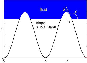
Figure 1: Fluid in contact with a substrate with cosines corrugation. The fluid occupy half the region where the absolute value of the slope is below $-\mathrm{tan}\theta$.

Let us first focus on the case where the fluid makes contact with a cosines profile $h(x,y)=h_{0}\mathrm{cos}(qx)$. In this case the contact will be as indicated in Fig. 1. If $-\mathrm{tan}\theta$ is larger than the maximum slope $qh_{0}=s_{0}\surd 2$, fluid will make complete contact with the solid (Wenzel state). However, if $-\mathrm{tan}\theta<qh_{0}$ we have the situation shown in Fig. 1. In this case the fluid will make contact with the solid in half of the surface region where the slope $s<-\mathrm{tan}\theta$ and we can write

$$\gamma^{*}_{\mathrm{SL}}=\int_{0}^{-\mathrm{tan}\theta}ds\ P(s)\left({\frac{1}{2}}\left(\gamma_{\mathrm{SL}}+\gamma_{\mathrm{SV}}\right)\left(1+s^{2}\right)^{1/2}+{\frac{1}{2}}\gamma_{\mathrm{LV}}\right)$$

$$+\int_{-\mathrm{tan}\theta}^{\infty}ds\ P(s)\left(\gamma_{\mathrm{SV}}\left(1+s^{2}\right)^{1/2}+\gamma_{\mathrm{LV}}\right)$$

and

$$\gamma^{*}_{\mathrm{SV}}=\gamma_{\mathrm{SV}}\int_{0}^{\infty}ds\ P(s)\left(1+s^{2}\right)^{1/2}$$

Combining (2), (7) and (8) and using (1) gives

$$\mathrm{cos}\theta_{0}=-1+{\frac{1}{2}}\int_{0}^{-\mathrm{tan}\theta}ds\ P(s)\left(\left(1+s^{2}\right)^{1/2}\mathrm{cos}\theta+1\right)$$

If $\theta$ is close to $\pi$ we have $-\mathrm{tan}\theta\approx 0$ and we can write (9) as

$$\mathrm{cos}\theta_{0}=-1+{\frac{1}{2}}\left(\mathrm{cos}\theta+1\right)\int_{0}^{-\mathrm{tan}\theta}ds\ P(s)$$

This equation was derived for a surface with a single cosines corrugation, but should hold approximately also for a randomly rough surface with roughness on a single length scale, i.e., a surface generated by the superposition of cosines waves (or plane waves) with equal wavelength but different propagation directions (in the $xy$-plane) and with different (random) phases. Such a surface will have the distribution of slopes given by (5). With $P(s)$ given by (5) from (10) we get

$$\mathrm{cos}\theta_{0}=-1+{\frac{1}{2}}\left(\mathrm{cos}\theta+1\right)\left(1-\mathrm{exp}\left[\left({\frac{\mathrm{tan}\theta}{s_{0}}}\right)^{2}\right]\right)$$

If we write $\theta_{0}=\pi-\phi_{0}$ and $\theta=\pi-\phi$ with $\phi_{0}<<1$ and $\phi<<1$ we get from (11)

$$\phi_{0}={\frac{\phi^{2}}{\surd 2s_{0}}}$$

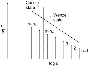
Figure 2: The solid line shows the power spectrum as a function of the wavevector (log-log scale) of a self-affine fractal surface with roughness over several decades in length scale. The power spectrum given by the vertical arrows (Dirac delta functions) correspond to a rough surface composed of a discrete set of wavelength components. We can consider this as a discretize version of the continuous power spectrum. We assume the separation between two nearby delta functions to be of order 1 decade in length scale.

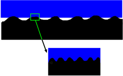
Figure 3: The interface between a fluid droplet and a rough substrate. At large length scales the liquid droplet will not make full contact with the rough surface (Cassie state). However, when an apparent contact area is magnified, it is observed that at shorter length scales the fluid is in complete contact with the roughness profile.

Consider a randomly rough surface with roughness on many length scales. Most solids have surface roughness which is approximately self-affine fractal over several decades in length scalesPersson (2014). A self affine fractal surface has a power spectrum which depends on the wavevector $q$ as a power law $C(q)\sim q^{-2(1+H)}$ where the Hurst exponent $0<H<1$. In addition, most surfaces have a roll-off region for $q<q_{\mathrm{r}}$. The solid line in Fig. 2 shows the power spectrum of such a surface. Here we consider instead a rough surface composed of a discrete set of wavelength components with the power spectrum given by the vertical arrows (Dirac delta functions) in Fig. 2. We can consider this as a discretize version of the continuous power spectrum in Fig. 2. We assume the separation between two nearby delta functions to be of order 1 decade in length scale. This large separation in length scales allow us to integrate out, or eliminate the roughness which occur at length scales shorter than the length scale under consideration.

We will now consider how the contact angle $\theta_{0}$ changes as we gradually add more roughness components to the surface profile. We will use a Renormalization Group type of picture and study how the effective interfacial energy $\gamma_{\mathrm{SL}}(n)$ (and $\gamma_{\mathrm{SV}}(n)$) change as we include more and more of the surface roughness components, i.e., we gradually increase $n$ from $n=1$ to the final value $n=n_{1}$ where all the roughness components are included (see Fig. 2). Consider first a surface where we only include the shortest wavelength roughness components (associated the $n=1$ Dirac delta function in Fig. 2). Weassume that the slope of the surface is everywhere below $-\mathrm{tan}\theta$. In this case fluid will make complete contact with the rough surface. If we now consider the system at a lower magnification the surface appear smooth and flat. The fluid contact angle at this magnification can be calculated from (3) with the modified (effective) interfacial energy:

$$\gamma_{\mathrm{SL}}(n=1)=\gamma_{\mathrm{SL}}\times r_{1}$$

where $r_{1}=A(n=1)/A_{0}$ is the ratio between the surface area $A(n=1)$ and the nominal surface area $A_{0}$. Using this effective interfacial energy, and a similar expression for $\gamma_{\mathrm{SV}}(n=1)$, from (3) one obtain the fluid droplet contact angle $\mathrm{cos}\theta(1)=r_{1}\mathrm{cos}\theta$.

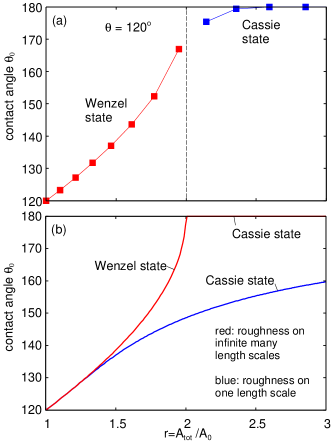
Figure 4: The contact angle $\theta_{0}=\theta(n)$ as a function of the parameter $r=A_{\mathrm{tot}}/A_{0}$. (a) The red symbols are the results obtained from the equation $\mathrm{cos}\theta(n)=r_{n}\mathrm{cos}\theta(n-1)$ with $n\leq n_{\mathrm{W}}$ (in the present case ($n\leq n_{\mathrm{W}}=7$) and the blue symbols using $\phi(n+1)=\phi^{2}(n)/(\surd 2s_{n})$ for $n>n_{\mathrm{W}}$. (b) The limiting case where roughness occur on infinite many length scales (upper curve) or on a single length scale (lower curve).

Let us now add the next shortest wavelength roughness components, represented by the Dirac delta function peek $n=2$ in Fig. 2. We assume that the slope of the surface is everywhere below $-\mathrm{tan}\theta(1)$. In this case fluid will make complete contact with the rough surface. If we now consider the system at a lower magnification the surface appear smooth and flat. The fluid contact angle at this magnification can be calculated from (3) with the modified (or effective) interfacial energy:

$$\gamma_{\mathrm{SL}}(n=2)=\gamma_{\mathrm{SL}}(1)\times r_{2}$$

where $r_{2}=A(n=2)/A(n=1)$ where $A(n=2)$ is the surface area obtained with the $n=1$ and $n=2$ roughness components. Using this effective interfacial energy, and a similar expression for $\gamma_{\mathrm{SV}}(n=2)$, from (3) one obtain the fluid droplet contact angle $\mathrm{cos}\theta(2)=r_{2}\mathrm{cos}\theta(1)$. More generally, we have

$$\mathrm{cos}\theta(n)=r_{n}\mathrm{cos}\theta(n-1)$$

where $r_{n}=A(n)/A(n-1)$. Eq. (13) is valid also for $n=1$ if we define $\theta(n=0)=\theta$ as the contact angle on the flat perfectly smooth surface, and $A(n=0)=A_{0}$. If the root-mean-square slope associated with the roughness in each of the Dirac delta functions peeks is small enough, the procedure described above can be continued until $\theta(n)$ is close to $\pi$ (or $180^{\circ}$) and we conclude that for a surface with roughness on many length scales the Wenzel state will prevail until the root-mean-square roughness is so high that the Wenzel equation predict a contact angle close to $\pi$. We define $n=n_{\mathrm{W}}$ as the smallest $n$ for which $r_{n_{\mathrm{W}}+1}\mathrm{cos}\theta(n_{\mathrm{W}})<-1$, at which point there is no solution to the Wenzel equation (Eq. (3)): $\mathrm{cos}\theta(n_{\mathrm{W}}+1)=r_{n_{\mathrm{W}}+1}\mathrm{cos}\theta(n_{\mathrm{W}})$

Consider now adding the $n=n_{\mathrm{W}}+1$ roughness component. Since the maximum surface slope associated with the $n=n_{\mathrm{W}}+1$ roughness component is larger than $-\mathrm{tan}\theta(n_{\mathrm{W}})$, the liquid droplet will not make full contact with the rough surface. However, at shorter length scales the fluid is in complete contact with the roughness profile as indicated in Fig. 3. To study the development of the contact angle as we add more roughness we assume that (9) is valid, which for $\theta=\pi-\phi\approx\pi$ takes the form (12) which we now write as

$$\phi(n+1)={\frac{\phi^{2}(n)}{\surd 2s_{n}}}$$

for $n\geq n_{\mathrm{W}}$, with $\phi(n_{\mathrm{W}})$ determined by the contact angle in the Wenzel state which prevail when $n=n_{\mathrm{W}}$. In (14) $s_{n}$ is the rms slope associated with the surface roughness contained in the $n$’th Dirac delta function (see Fig. 2). Note that for a randomly rough surface $s_{n}$ can be calculated from $r_{n}$.

We now present numerical results to illustrate the discussion above. Assume that the fluid contact area on the flat smooth surface equals $\theta=120^{\circ}$ as would be typical for Teflon. Assume that $r_{1}=r_{2}=..=1.1$. This correspond to $s_{1}=s_{2}=...\approx 0.46$. Note that the total surface area after adding the first $n$ roughness wavelength components is $A_{\mathrm{tot}}/A_{0}=r_{1}\times r_{2}\times...\times r_{n}$. In Fig. 4(a) we show the contact angle $\theta_{0}=\theta(n)$ as a function of the parameter $r=A_{\mathrm{tot}}/A_{0}$.

It is instructive to consider two limiting cases, namely the case where surface roughness occur over infinite decades in length scales (this limit can of course not be realized in reality as it is meaningless to consider roughness at length scales below the atomic dimension) and when roughness occur on a single length scale. In the former case, we assume as above a surface roughness power spectrum consisting of Dirac delta function peaks separated by $\sim 1$ decade in lengthscale. We consider a surface with a finite rms slope and we assume that each Dirac delta function contribute equally to the rms slope. Hence since there are infinite many Dirac delta functions each of them must have an infinitesimal weight corresponding to roughness with infinitesimal amplitude. It is clear that in this case the condition $r_{n_{\mathrm{W}}+1}\mathrm{cos}\theta(n_{\mathrm{W}})<-1$ will be satisfied only when the contact angle $\theta(n_{\mathrm{W}})$ differ from $\pi$ by an infinitesimal amount, i.e., the Wenzel state will prevail (minimum free energy state) until $r$ is so large that Eq. (3) predict $\theta=\pi$ after which the Cassie state will prevail (with $\theta=\pi$).

For the second limiting case of roughness on a single length scale we use (11) to estimate the contact angle $\theta_{0}$ for the Cassie state. In Fig.4(b) we show the contact angles for these two limiting cases.

We now present results for the contact angle as a function of the roughness parameter $r$ based on an exact numerical treatment of an one-dimensional (1D) model. Using standard procedures (see, e.g., Appendix D in Ref. Persson et al. (2005)) we have generated randomly rough 1D surfaces and studied the fluid contact angle using the method described in Ref Bottiglione and Carbone (2015). We consider surfaces with roughness extending over what we denote as a “narrow” and a “wide” range of length scales. The roughness power spectral density (PSD) $C(q)$ of the two types of surfaces are shown in Fig. 5. Both surfaces have the rms slope 0.25 and Hurst exponent $H=0.8$, but different large wavevector cut-off. As a result, the rms roughness is larger for the surface with the more narrow PSD. This is illustrated in Fig. 6 which shows the height distribution $P_{h}$ of both surfaces.

We will show below that in spite of the larger rms roughness amplitude of the surface with the more narrow PSD, the (apparent) contact angle is largest on the surface with the widest PSD. This shows that the rms roughness is irrelevant for the contact angle which instead is determined by the rms slope and how different length scales contribute to the rms slope.

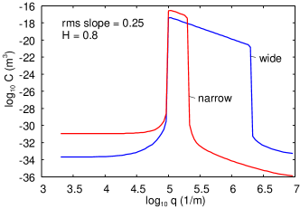
Figure 5: The surface roughness power spectra $C(q)$ of surfaces with the rms slope 0.25 and Hurst exponent $H=0.8$ but different large wavevector cut-off.

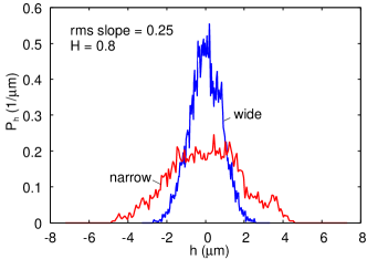
Figure 6: The height distribution $P_{h}$ of surfaces with the rms slope 0.25 and Hurst exponent $H=0.8$ but different large wavevector cut-off.

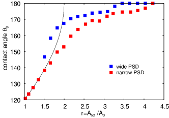
Figure 7: The contact angle $\theta_{0}$ as a function of the parameter $r=A_{\mathrm{tot}}/A_{0}$ obtained from numerical simulations. The solid line is given by the Wenzel equation (3).

Fig. 7 shows the contact angle $\theta_{0}$ as a function of the parameter $r=A_{\mathrm{tot}}/A_{0}$ obtained from numerical simulations. Note that the surface with the more wide distribution of roughness lengthscales has larger contact angle in spite of the fact that both surfaces have the same rms slope. In general, several metastable droplet states are possible, and which state occur depends on the preparation procedure. We note, however, that the minimum free energy state is the state with the lowest contact angle. Thus, the Cassie states observed for $r<2$ in Fig. 7 are metastable states, and the ground state is in this case the Wenzel state. In the theory presented above we assumed that the system was in the minimum free energy state and no Cassie state could occur above the Wenzel line for $r<2$.

The result in Fig. 7 is consistent with the theory prediction presented in Fig. 4. In the numerical simulations the contact angle in the Cassie state is smaller than in the theory, but this reflects the fact that the roughness occur over a wider range of length scales in the theory as compared to the numerical model. This is indeed confirmed by numerical calculations presented by the authors in Bottiglione and Carbone (2015) (see Fig. 10 therein) where the surface roughness was characterized by a much larger number of length scales covering about 3 decades.

To summarize, we have shown when the number of length scales of roughness increases, the transition from the Wenzel state to the Cassie state approach the threshold value $r=A_{\mathrm{tot}}/A_{0}=-1/\mathrm{cos}\theta$, and the contact angle in the Cassie state approaches $180^{\circ}$.

References

- Liu and Jiang (2012) K. Liu and L. Jiang, Annual Review of Materials Research 42, 231 (2012).
- Varanasi et al. (2010) K. K. Varanasi, T. Deng, J. D. Smith, M. Hsu, and N. Bhate, Applied Physics Letters 97, 234102 (2010).
- Meuler, McKinley, and Cohen (2010) A. J. Meuler, G. H. McKinley, and R. E. Cohen, ACS nano 4, 7048 (2010).
- Rothstein (2010) J. P. Rothstein, Annual Review of Fluid Mechanics 42, 89 (2010).
- Ming et al. (2011) Z. Ming, L. Jian, W. Chunxia, Z. Xiaokang, and C. Lan, Soft Matter 7, 4391 (2011).
- Gao et al. (2007) X. Gao, X. Yan, X. Yao, L. Xu, K. Zhang, J. Zhang, B. Yang, and L. Jiang, Advanced Materials 19, 2213 (2007).
- Li, Zhang, and Yang (2010) Y. Li, J. Zhang, and B. Yang, Nano Today 5, 117 (2010).
- Zhu et al. (2009) J. Zhu, C.-M. Hsu, Z. Yu, S. Fan, and Y. Cui, Nano letters 10, 1979 (2009).
- Gau et al. (1999) H. Gau, S. Herminghaus, P. Lenz, and R. Lipowsky, Science 283, 46 (1999).
- Blossey (2003) R. Blossey, Nature materials 2, 301 (2003).
- Nakajima et al. (1999) A. Nakajima, A. Fujishima, K. Hashimoto, and T. Watanabe, Advanced Materials 11, 1365 (1999).
- Deng et al. (2012) X. Deng, L. Mammen, H.-J. Butt, and D. Vollmer, Science 335, 67 (2012).
- Barthlott and Wilhelm (1977) W. Barthlott and E. Wilhelm, Akad. Wiss. Lit. Mainz 19 (1977).
- Barthlott and Neinhuis (1997) W. Barthlott and C. Neinhuis, Planta 202, 1 (1997).
- Gao and Jiang (2004) X. Gao and L. Jiang, Nature 432, 36 (2004).
- Cassie and Baxter (1944) A. Cassie and S. Baxter, Transactions of the Faraday Society 40, 546 (1944).
- Quéré, Lafuma, and Bico (2003) D. Quéré, A. Lafuma, and J. Bico, Nanotechnology 14, 1109 (2003).
- Afferrante and Carbone (2014) L. Afferrante and G. Carbone, Soft Matter 10 (2014).
- Afferrante and Carbone (2010) L. Afferrante and G. Carbone, Journal of Physics: Condensed Matter 22, 325107 (2010).
- Carbone and Mangialardi (2005) G. Carbone and L. Mangialardi, The European Physical Journal E - Soft Matter 16, 67 (2005).
- Forsberg, Nikolajeff, and Karlsson (2011) P. Forsberg, F. Nikolajeff, and M. Karlsson, Soft Matter 7, 104 (2011).
- Emami et al. (2011) B. Emami, H. V. Tafreshi, M. Gad-el Hak, and G. Tepper, Applied Physics Letters 98, 203106 (2011).
- Moulinet and Bartolo (2007) S. Moulinet and D. Bartolo, The European Physical Journal E 24, 251 (2007).
- Yang, Tartaglino, and Persson (2008) C. Yang, U. Tartaglino, and B. N. J. Persson, The European Physical Journal E 25, 139 (2008).
- Yang, Tartaglino, and Persson (2006) C. Yang, U. Tartaglino, and B. N. J. Persson, Physical review letters 97, 116103 (2006).
- Richard and Quéré (2000) D. Richard and D. Quéré, EPL (Europhysics Letters) 50, 769 (2000).
- Wenzel (1949) R. N. Wenzel, The Journal of Physical Chemistry 53, 1466 (1949).
- Lafuma and Quéré (2003) A. Lafuma and D. Quéré, Nature materials 2, 457 (2003).
- Koishi et al. (2009) T. Koishi, K. Yasuoka, S. Fujikawa, T. Ebisuzaki, and X. C. Zeng, Proceedings of the National Academy of Sciences 106, 8435 (2009).
- Verho et al. (2012) T. Verho, J. T. Korhonen, L. Sainiemi, V. Jokinen, C. Bower, K. Franze, S. Franssila, P. Andrew, O. Ikkala, and R. H. Ras, Proceedings of the National Academy of Sciences 109, 10210 (2012).
- Boreyko et al. (2011) J. B. Boreyko, C. H. Baker, C. R. Poley, and C.-H. Chen, Langmuir 27, 7502 (2011).
- Li and Amirfazli (2008) W. Li and A. Amirfazli, Soft Matter 4, 462 (2008).
- Su et al. (2010) Y. Su, B. Ji, K. Zhang, H. Gao, Y. Huang, and K. Hwang, Langmuir 26, 4984 (2010).
- Koch, Bohn, and Barthlott (2009) K. Koch, H. F. Bohn, and W. Barthlott, Langmuir 25, 14116 (2009).
- Onda et al. (1996) T. Onda, S. Shibuichi, N. Satoh, and K. Tsujii, Langmuir 12, 2125 (1996).
- Shibuichi et al. (1996) S. Shibuichi, T. Onda, N. Satoh, and K. Tsujii, The Journal of Physical Chemistry 100, 19512 (1996).
- Bottiglione et al. (2015) F. Bottiglione, R. Di Mundo, L. Soria, and G. Carbone, Nanoscience and Nanotechnology Letters 7 (2015).
- Bottiglione and Carbone (2015) F. Bottiglione and G. Carbone, Journal of Physics: Condensed Matter 27 (2015).
- Di Mundo, Bottiglione, and Carbone (2014) R. Di Mundo, F. Bottiglione, and G. Carbone, Journal of Physics: Condensed Matter 316 (2014).
- Bottiglione and Carbone (2012) F. Bottiglione and G. Carbone, Langmuir 29, 599 (2012).
- Flemming, Coriand, and Duparré (2009) M. Flemming, L. Coriand, and A. Duparré, Journal of Adhesion Science and Technology 23, 381 (2009).
- Awada et al. (2010) H. Awada, B. Grignard, C. Jérôme, A. Vaillant, J. De Coninck, B. Nysten, and A. M. Jonas, Langmuir 26, 17798 (2010).
- David and Neumann (2012) R. David and A. W. Neumann, The Journal of Physical Chemistry C 116, 16601 (2012).
- Persson and Tosatti (2001) B. N. J. Persson and E. Tosatti, Journal of Chemical Physics 115 (2001).
- Persson (2014) B. N. J. Persson, Tribology Letters 54 (2014).
- Persson et al. (2005) B. N. J. Persson, O. Albohr, U. Tartaglino, A. I. Volokitin, and E. Tosatti, Journal of Physics: Condensed Matter 17, R1 (2005).