Rigidity of Melting DNA

Abstract

The temperature dependence of DNA flexibility is studied in the presence of stretching and unzipping forces. Two classes of models are considered. In one case the origin of elasticity is entropic due to the polymeric correlations, and in the other the double-stranded DNA is taken to have an intrinsic rigidity for bending. In both cases single strands are completely flexible. The change in the elastic constant for the flexible case due to thermally generated bubbles is obtained exactly. For the case of intrinsic rigidity, the elastic constant is found to be proportional to the square root of the bubble number fluctuation.

I Introduction

To facilitate different fundamental biological processes, like replication, gene expression, assembly of functional nucleoprotein structures, and packaging of viral DNA, DNA has to go through a lot of twisting, stretching, and bending bend-1 ; bend-2 ; giese ; schultz ; nagaich ; ortega ; watson . Generally different proteins induce these conformational changes in DNA, but not without facing any resistance. This is because, when subjected to an external mechanical force, DNA responds elastically. Single-stranded DNA may be flexible and easy to bend, but double-stranded DNA (dsDNA) is known to be more rigid. However, the flexibility of short DNA fragments is important for different in vivo mechanisms, like those already mentioned, where loops or bends as short as 100 base pairs in length are involved bend-3 ; bend-4 , and also in in vitro experiments, where fragments are used in open or hairpin geometries. It is therefore important to probe the elastic response of dsDNA not only in the thermodynamic limit of long length — dsDNA is long — but also for finite-size systems.

Topological arguments, a la the Călugăreneau theorem volod , indicate the necessity of two major elastic constants of dsDNA, namely, the twist and the bending elastic constants. The former is tied to the helical nature of the double-helix and the latter is determined by both entropy and angular interactions between neighboring tangent vectors. These elastic moduli are characteristics of the bound phase and they disappear on DNAs melting into the denatured phase. It is quite analogous to the disappearance of the shear elastic modulus of a crystalline solid upon melting into the liquid phase. If dsDNA is treated as a free Gaussian polymer with noninteracting monomers, even then it exhibits an entropic elasticity originating from the correlations of a random walk. On the other hand, an intrinsic rigidity against bending at short scales (a semi flexible chain) produces a temperature dependent persistence length ($\sim 150$ base pairs), within which a dsDNA acts more or less like a rigid rod. Thus, it seems, a larger force is required to bend DNA of a length shorter than its persistence length than DNA of a longer length doi ; smb-flory . Recent debates cloutier ; wiggins ; yanmarko ; menon ; menon1 ; qdu ; mazur ; noy ; linna ; shroff ; forties ; le ; kramenetskii on the behavior of short segments brought into focus the importance of broken base pairs on its eventual or effective rigidity. As the base-pair energy is comparable to the thermal energy at physiological temperatures ($\sim$2-3 kcal/mol), bubbles form spontaneously or are produced by external forces (see, e.g., bubble-force for an earlier study). Consequently, the issue of the elastic response of dsDNA cannot be studied in isolation as its intrinsic property but rather needs to be coupled to the inner degrees of freedom, namely, base pairings responsible for the bound state.

Breaking the base pairings can separate dsDNA into two independent single strands and this melting happens at a particular temperature. The thermal melting of DNA is by itself an interesting problem and important for different in vivo or in vitro processes. A notable example is the polymer chain reaction, which is used extensively in DNA amplification. Other than that it has been proposed efimov1 ; efimov2 ; efimov3 that at the dsDNA melting point the addition of a third strand may support a three-stranded DNA bound state where no two pairs of strands are expected to be bound. This novel three-stranded DNA bound state is called Efimov-DNA and has been shown to support a renormalization-group limit cycle tp1 ; tp2 . In the temperature region below the melting point there can be local melting at different positions, creating denaturation bubbles, which are nothing but single stranded loops preceded and succeeded by double-stranded segments. As single-stranded DNA is far more flexible than paired ones, these thermally generated bubbles can provide flexible hinges which can make dsDNA significantly flexible yanmarko ; menon ; menon1 . Generally the average length of these bubbles increases as the critical point is approached and equals the system length at the melting temperature. The importance of bubbles for the melting transition is well understood in the Poland-Scheraga framework poland . The entropic contributions of the bubbles in different models, originating from long range polymeric correlations of the individual strands, lead to different types of melting behavior, from weakly first order to infinite order peyrard1 ; peyrard2 ; peyrard3 ; prakash ; efimov1 ; efimov2 ; efimov3 ; tp1 ; tp2 ; poland ; kafri1 ; kafri2 ; trovato ; marenduzzo ; azbel . The simpler coarse-gain level models show critical behavior poland ; peyrard1 ; peyrard2 ; peyrard3 ; trovato ; fisher ; tp1 ; tp2 ; sutapa ; poulomi . Close to melting, the bubbles are therefore expected to contribute significantly to the flexibility, beyond just acting as hinges. Different from thermal melting is the unzipping transition, where the two strands of dsDNA are pulled apart at temperatures below the melting point. The unzipping transition is generally first order smb-unzip ; poulomi , even in models with a first order melting transition kafri1 ; kafri2 . Since the unzipping force does not penetrate the bound state poulomi ; skumar , the nature of the bubble distribution does not change in the presence of an unzipping force. As a result, the bubbles are going to have their signatures on the flexibility of a DNA near the unzipping transition too. From a phase transition point of view, the bending elastic constant, despite its importance for DNA activity, is not a primary response function that characterizes a critical point. For example, one may compare it with the magnetic susceptibility of a ferro-para magnetic transition or the elastic modulus in a liquid-gas transition, whose divergence is associated with an exponent $\gamma$. But as it is not the primary response function, no such general results of critical phenomena are applicable here. Hence the necessity for a detailed study of the rigidity of melting DNA. In this paper we want to explore the elastic properties of DNA near its melting point. DNA melting is a genuine phase transition for which the DNA length has to satisfy the thermodynamic limit. But still, the existence of a transition point is sufficient to affect a finite-size system even when it is away from the critical point. One of our aims is to obtain a few exact results on the elastic behavior for a class of models of DNA melting and unzipping.

Different statistical mechanical models have been applied with varying success to study the DNA elasticity problem. The classical semiflexible chain model with no denaturation bubbles has been employed by a number of investigators zimm ; seol . Segments made of single strands can be introduced in discretized semiflexible DNA, by considering models comprised of two-state internal coordinates and, also, by coupling these internal coordinates to the external rotational degrees of freedom of its tangent vectors nikos ; kwlc ; palmeri . Bubbles appear naturally in our models without utilizing any other secondary variables.

The modulus of interest comes from the response to a force applied at one end of each of the two strands, keeping the other end fixed at the origin. We use models of DNA where the strands are represented as polymers with native base pairing; namely, two monomers of the two strands interact only when they have the same contour length on the polymer. To probe the elastic behavior, we use a stretching force that would act on both strands in the same direction, while the phase can be changed by an unzipping force that acts on the strands in opposite directions. Here we quantitatively relate DNA flexibility to bubble-related quantities such as the bubble length, the bubble number etc.

The organization of this paper is as follows. In Sec. II, we qualitatively describe the models, the flexible model and the rigid model, considered in this paper. Section III is devoted to the flexible model. In Sec. III.1, we introduce the corresponding recursion relations and define the observables necessary for analysis of both models. The elastic properties of the flexible model are explored in Sec. III.2, where we show a finite discontinuity in the elastic modulus at the melting point. We obtain the phase diagram in the presence of an unzipping force and a stretching force in Sec. III.4. The transition is now first order and the elastic modulus shows a $\delta$-function peak at the transition point. We introduce the rigid model in Sec. IV. After listing its governing recursion relations and defining the required observables specific to this model, we obtain its thermal melting (a continuous transition) point in Sec. IV.1. In Sec. IV.2, we show that the corresponding elastic modulus becomes anomalous around the melting point as it surpasses the unbound-state elastic modulus. The roles played by the bubbles are shown quantitatively in Sec. IV.3. Only the stretching force is considered for the rigid model. After a brief discussion of the relevance of our results in Sec. V, we summarize and conclude in Sec. VI. A few important supplementary materials are listed in the Appendices A and B.

II Qualitative Description

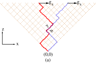
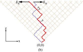
Figure 1: (color online). Schematic of dsDNA as two directed walks in the $(1+1)$ dimension. The direction in which the forces act are indicated by arrows. (a) Flexible model : The polymers can not cross each other. The bound segments can bend left or right freely. This freedom can be restricted by introducing a statistical weight $b$. Here, $b$ is associated with the left degree of freedom. (b) Rigid model : The polymers can cross here. The bound segments can not bend to the right and they are at least two bonds long. $v$ is the weight associated with the bubble opening or closure.

To isolate the entropic and the intrinsic elastic behavior, two types of models are considered, viz., a flexible model, the standard model used for melting and unzipping marenduzzo ; rajeev12 ; rajeev11 ; trovato ; rajeev , and a rigid model, built from the flexible model. See Fig. 1. Both models show a zero-force melting point, generically denoted $y_{c}$. The common features of these models are as follows : we consider each single strand as a directed polymer in a two-dimensional square lattice. We represent the base pairing by contact interactions between the monomers which can only occur at the same space and length coordinates. Correct base-pair bonding is ensured by the directedness of the polymers. The chains are inextensible sdna , of the same length, and attached to each other at the origin. We mimic DNA melting by the binding-unbinding phase transition in the system. The statistical weight of a contact interaction is the Boltzmann factor $y=\exp(\beta\epsilon)$, $-\epsilon$ being the energy per contact and $\beta$ the inverse temperature with the Boltzmann constant set to $k_{B}=1$. Such models in the past have been instrumental in studies of the melting and the unzipping transition of dsDNA and are known to show the relevant features of the higher dimensional models smb-unzip ; trovato ; rajeev11 ; rajeev12 . These models are also useful for studies of the dynamics of DNA. The flexible model [Fig. 1(a)] has a hard-core repulsion that forbids the two chains to cross. The perfectly bound DNA remains as flexible as the single-stranded DNA so that at any nonzero temperature there is only the emergent entropic elasticity. In contrast, the rigid model [Fig. 1(b)] has a bound state which has an intrinsic rigidity towards or against bending. In fact we consider the dsDNA to be absolutely rigid in the bound state. The only way it can show any flexibility is via denaturation bubbles. Thus, the elastic response in this model is purely due to the flexible hinges made accessible by the bubbles. It is possible to allow some controlled semiflexibility, instead of absolute rigidity, via the introduction of a parameter $b$, which penalizes the bound DNA taking an unfavorable turn. This model is discussed the Appendix B. This imposed rigidity is enough to give a melting transition even in the absence of any hard-core constraint. To incorporate this rigidity unambiguously, a constraint is required that a bound base pair can form only if its previous monomers are in the bound state.

We apply an external space-independent mechanical stretching force independently at the end of each strand. If the two forces are in the same direction, the dsDNA is said to be under a stretching force $g_{s}$. On the other hand, it will be under an unzipping force $g_{u}$ if the forces are in opposite directions. The average extension and the elastic modulus can be obtained from the free energy simply by taking derivatives with respect to the stretching force once and twice, respectively.

We use the transfer matrix method through recursion relations to find the partition function of the system. For the analytical solution, the generating function for the grand partition function is used, from whose singularities the free energy can be determined marenduzzo . For numerical calculations we iterate the recursion relations for finite lengths and find the exact partition function. The numerical calculations reflect the finite-size behavior of the concerning quantities. The effect of the unzipping force in the elasticity is also explored. The general case of two unequal forces can always be transformed into a case of unzipping and stretching forces. Since unzipping and stretching of dsDNA are independent of each other, we are able to generate a general phase diagram for three variables: the temperature, the stretching force, and the unzipping force.

III Flexible Model

We use the model from Ref. rajeev introduced to study the unzipping transition of dsDNA discussed in the last section. First, we solve the model analytically through the generating function technique, and then we study numerically the behavior of finite-length systems.

III.1 Recursion relation and observables

In the absence of any force the recursion relation followed by this system is given by rajeev :

$$Z_{n+1}(x_{1},x_{2})=\sum_{(i,j)=\pm 1}Z_{n}(x_{1}+i,x_{2}+j)[1-(1-y)\delta_{x_{1},x_{2}}],$$ (1)

where $Z_{n}(x_{1},x_{2})$ is the canonical partition function of the system of two polymers, each of length $n$, and the spatial positions of the $n$th monomers of polymer $1$ and polymer $2$ are $x_{1}$ and $x_{2}$, respectively. For a given monomer number if $x_{1}$ becomes equal to $x_{2}$, then there is a contact. We set the initial condition as $Z_{0}(0,0)=y$ such that two strands start from the origin. The non-crossing constraint is implemented by not letting $x_{1}$ becoming greater than $x_{2}$ $(x_{1}\leq x_{2})$.

We apply a constant stretching force $g_{s}$ at the open end point of each strand. The partition function of $n$-length DNA in the presence of this stretching force is given by

$${\sf Z}(g_{s})=\sum_{x_{1},x_{2}}Z_{n}(x_{1},x_{2})e^{g_{s}X},\hskip 7.22743pt\text{where}\hskip 7.22743ptX=x_{1}+x_{2}$$ (2)

and the sum is over all the allowed values of $x_{1}$ and $x_{2}$.

The elastic response of the system under a stretching force can be quantified through the average extension $(x)$ and the elastic modulus $(\kappa)$. We define them in the following way

$$x=\frac{\partial f}{\partial g_{s}}=\frac{1}{N}\frac{\partial\ln{\sf Z}(g_{s})}{\partial g_{s}},\hskip 7.22743pt\text{and}\hskip 7.22743pt\kappa=\frac{\partial x}{\partial g_{s}},$$ (3)

where $f=\beta F=-\ln Z(g_{s})$ is the free energy of the system scaled by $\beta$, and $N$ is the length of the strands $(N\to\infty)$. Using Eq. (2) we can rewrite them as

$$x = \frac{\langle X\rangle}{N}=\frac{\sum_{x_{1},x_{2}}Z_{N}(x_{1},x_{2})e^{g_{s}X}X}{N\sum_{x_{1},x_{2}}Z_{N}(x_{1},x_{2})e^{g_{s}X}},$$ (4a)

$$\kappa = \frac{1}{N}\left(\langle X^{2}\rangle-\langle X\rangle^{2}\right),$$ (4b)

where $\langle...\rangle$ denotes the thermal average as indicated in Eq. (4a). An inspection of Eqs. (4a) and (4b) shows that $x$ is related to the average vectorial position of the center of mass of the end points of the two strands of length $n$ under a stretching force $g_{s}$, and as expected, $\kappa$ is related to the fluctuation of $x$. If $x_{1}$ and $x_{2}$ are uncorrelated, then $\kappa$ is the sum of the individual elastic constants. This will be the case in the unbound phase. According to this definition for a given force the larger the value of $\kappa$, the greater is the flexibility of the dsDNA. Two other important quantities are the average number of contacts between two strands $(n_{c})$ and its fluctuation $(C_{c})$. Two extreme values of $n_{c}$, 0 and 1, represent the unbound and the bound states, respectively. As $y$ is a temperature-like variable one can derive the specific heat of the system from $C_{c}$. We call it the specific heat for brevity. These are defined as

$$n_{c}=\frac{y}{N}\frac{\partial f}{\partial y}\hskip 7.22743pt\text{and}\hskip 7.22743ptC_{c} = y\frac{\partial n_{c}}{\partial y}.$$ (5)

We follow these definitions in the rest of this paper.

The recursion relations defined above can be solved exactly in the infinite-chain limit (i.e., the thermodynamic limit) with the help of generating functions. Based on the closed-form expressions, the physical quantities are obtained by taking appropriate derivatives as in Eq. (3). The results obtained in this way are called “analytical results.” These recursion relations can also be evaluated exactly, but numerically, by using the transfer matrix technique, for finite-length chains. The physical quantities like the average extension and elastic modulus are then obtained by using Eqs. (4a) and (4b). To evaluate $n_{c}$ and $C_{c}$ numerically we need to find out the first and the second numerical derivatives of the partition function with respect to $y$. We evaluate the recursion relations for the first and the second derivatives of the zero-force partition function by taking the first and second derivatives of Eq. (1) with respect to $y$, respectively, and iterate them numerically to evaluate them. Then, using Eq. (5) we calculate $n_{c}$ and $C_{c}$ for zero applied force. For a constant nonzero applied force, we follow the same procedure but evaluate the partition function and its $y$ derivatives by using Eq. (2) and taking derivatives of Eq. (2) with respect to $y$. Such exact numerical results below are to called “numerical results.”

III.2 Elastic Response Under a Stretching Force

Figure 2: (color online). Flexible model : Phase diagram of the system under a stretching force. The phase boundary separates the bound phase from the unbound phase. In the region $4/3>y>1$ there exists a critical $g_{sc}$ for every value of $y$ . Above $y=4/3$ the system is by default in the bound state. The solid blue line is the analytical curve, Eq. (11), and the red squares represent the numerically obtained critical points [see discussion following Eq. (17)].

III.2.1 Generating function and the free energy

By employing the generating function technique the recursion relation Eq. (1) can be exactly solved. We define

$$G(z,x_{1},x_{2})=\sum_{n=0}^{\infty}z^{n}Z_{n}(x_{1},x_{2}).$$ (6)

By doing this we are going to the grand-canonical ensemble from the canonical ensemble. By multiplying both sides of Eq. (1) by $z^{n}$ and then summing over $n$ we get two independent equations: one for nonzero unequal values of $x_{1}$ and $x_{2}$, and another for $x_{1}=x_{2}=0$. These are given by

$$\frac{1}{z}G(z,x_{1},x_{2}) = \sum_{(i,j)=\pm 1}G(z,x_{1}+i,x_{2}+j),$$ (7a)

$$\frac{1}{yz}G(z,0,0) = \frac{1}{z}+\sum_{(i,j)=\pm 1}G(z,i,j).$$ (7b)

The free energy per unit length of the DNA is determined by the singularity of $G(z,x_{1},x_{2})$ closest to the origin in the complex $z$-plane.

Assuming a power-law form for $G(z,x_{1},x_{2})$ with respect to the relative position coordinate we make the ansatz

$$G(z,x_{1},x_{2})=A(g_{s},z)\lambda(g_{s},z)^{(x_{1}-x_{2})/2}e^{g_{s}(x_{1}+x_{2})},$$ (8)

where $A$ and $\lambda$ are functions of $z$ and independent of position coordinates. Equation (8) generalizes the ansatz in Ref. rajeev . Using the ansatz, Eq. (8), in Eq. (7a) and Eq. (7b), two unknowns, $A(g_{s},z)$ and $\lambda(g_{s},z)$, can easily be solved. Their forms are given in Appendix A. The free energies of the different phases of the system are obtained from the singularities of $G(g_{s},z)$. The singularity $z_{b}$ of $A(g_{s},z)$ corresponds to the bound-state free energy and the branch point singularity $z_{f}$ of $\lambda(g_{s},z)$ gives the free energy of the unbound state. They are calculated as

$$z_{b}(y,g_{s}) = \frac{y-1}{y\ \text{sech}(2g_{s})}\left[\sqrt{\frac{\text{sech}^{2}(2g_{s})}{y-1}+1}-1\right],$$ (9a)

$$z_{f}(y,g_{s}) = \frac{\text{sech}^{2}(g_{s})}{4}.$$ (9b)

The difference in the force term can be understood by looking at the low-energy excitations. In the case of the free chains a force $g_{s}$ flips a bond interchanging the energies $\pm g_{s}$. This gives the $\text{sech}^{2}(g_{s})$ term. In the bound state, with coincident end points, a bound bond gets flipped under a force $2g_{s}$, yielding the $\text{sech}^{2}(2g_{s})$ term. From here onwards we suppress $y$ and $g_{s}$ as arguments for notational simplification and show them whenever necessary. The corresponding dimensionless free energies per unit length are given by

$$f_{b} = \ln z_{b},$$ (10a)

$$f_{f} = \ln z_{f}.$$ (10b)

There are two parameters in this formulation, $y$ and $g_{s}$. The singularities move when these two parameters are changed. Consider a situation where the system is in the bound state with the free energy given by $f_{b}$. Now, we can vary the parameters in such a way that the unbound-state singularity $z_{f}$ crosses $z_{b}$ and becomes closest to the origin. In this situation the free energy of the system becomes $f_{f}$. The crossing of the singularities defines the transition point from bound to unbound by the force at

$$g_{sc}=\frac{1}{2}\cosh^{-1}\left(\frac{2-y}{2(y-1)}\right).$$ (11)

The phase diagram in the $y$-$g_{sc}$ plane is shown in Fig. 2. The phase boundary has the following limiting forms:

$$g_{sc} \sim \sqrt{y_{c}-y}\hskip 14.45377pt\text{for}\hskip 14.45377pty\rightarrow y_{c}-,\hskip 14.45377pt\text{and}$$ (12a)

$$g_{sc} \sim -\frac{\ln(y-1)}{\ln y}\hskip 14.45377pt\text{for}\hskip 14.45377pty\rightarrow 1+.$$ (12b)

III.2.2 Results and discussions

Long-chain limit.

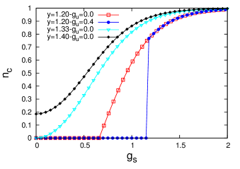
Figure 3: (color online). Flexible model : Variation of $n_{c}$ with $g_{s}$ for different values of $g_{u}$ and $y$. A non-zero $n_{c}$ indicates a bound state. For $g_{u}=0$, there is no unbound state for $y\geq 4/3$. The $g_{u}=0$ curves are from Eqs. (5), (10a), and (10b). The cyan line with triangles is for the melting point $y=y_{c}$, and shows the quadratic dependence on $g_{s}$. The black curve with filled diamonds represents $y=1.4>y_{c}$. The red curve, for $g_{u}=0$, shows a continuous transition, while the blue curve, for nonzero $g_{u}$, Eq. (21), shows a discontinuity. The symbols on these analytically obtained curves, in the infinite-chain limit, are to make them distinct.

When the two strands are in the unbound state, they come closer and form contacts in the influence of the stretching force. In this way an unbound state becomes a bound state above the critical stretching force. Figure 3 shows how $n_{c}$, calculated using Eq. (5), becomes non-zero before saturating at 1 as the stretching force crosses a critical value for a $y<y_{c}$. This shows that the transition is continuous. It is already known that at the point $(4/3,0)$ in the phase diagram the system goes through a second-order phase transition. Beyond this critical point the system always remains in the bound state, thus excluding any other possibilities of phase transition. The only effect of the stretching force there is to influence the bubble statistics. The asymptotic behavior of $n_{c}$ is given by

$$n_{c}\approx\begin{cases}\frac{9}{2}(g-g_{sc})\sqrt{y-y_{c}},&{\rm for\ }\genfrac{}{}{0.0pt}{}{y\to y_{c}+,}{g_{s}\to g_{sc}+,}\\ \frac{3}{2}\ g_{s}^{2},&{\rm for\ }y=y_{c},g_{s}\to 0,\\ n_{0}+\frac{g_{s}^{2}}{\sqrt{y(y-1)}},&{\rm for\ }y>y_{c},g_{s}\to 0,\\ \frac{27}{8}\left(y-y_{c}\right),&{\rm for\ }y\to y_{c}+,g_{s}=0,\end{cases}$$ (13)

where

$$n_{0}=n_{c}(y>y_{c},g_{s}=0)=\frac{y-2+\sqrt{y(y-1)}}{2(y-1)}.$$ (14)

That this is a second-order phase transition can be corroborated by examining the average extension of the center of mass due to the application of the stretching force and the elastic modulus. They are calculated using the definitions of Eq. (3).

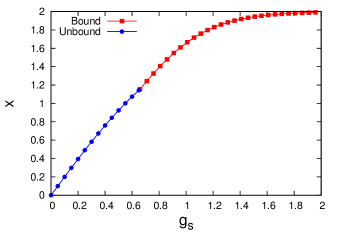
Figure 4: (color online). Flexible model : Plot of the average extension as a function of the stretching force with a fixed $y=1.20$. These are obtained from Eqs. (3), (10a), and (10b). The average extension varies continuously around the critical point. The symbols on these analytically obtained curves are to make them distinct.

Figure 4 shows how the average extension changes continuously as the system crosses the critical stretching force. For a zero force $x$ is 0, consistent with the Gaussian chain behavior, while the fully stretched state under a large force has $x=2$.

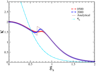
Figure 5: (color online). Flexible model : Elastic modulus curve for $y=1.20$. The solid brown line is the analytically obtained curve (see text). The dashed cyan line is for $\kappa_{b}=4\ \text{sech}^{2}(2g_{s})$, Eq. (18a), for the case with no bubbles. Other curves are the plots of $\kappa$ for different system lengths. Solid lines through the data points are guides for the eye.

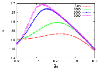
Figure 6: (color online). Flexible model : A magnified version of Fig. 5 around the same crossing point of all the curves. The chain length for each curve is given in the legend. Solid lines through the data points are guides for the eye.

The slope discontinuity at the transition point $g_{sc}$ of Eq. (11) gives rise to a jump in the elastic constant as shown in Fig. 5. To be noted here is that there is no pretransitional signature on either side of the transition.

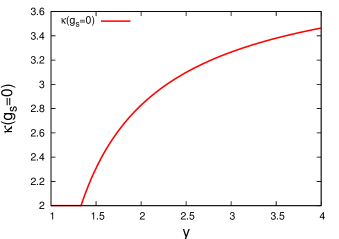
Figure 7: (color online). Flexible model: The elastic modulus, Eq. (15), as a function of $y$ for zero stretching force.

However, for a finite-size system the scenario is different. All other curves in Fig. 5 except the analytical curve are for different finite sizes of the system. In the unbound phase each strand has the equation of state $x=\tanh(g_{s})$ so that the total $x=2\tanh(g_{s})$. This is the $g_{s}<g_{sc}$ branch. The corresponding entropic elastic constant is $\kappa=2\ \text{sech}^{2}(g_{s})$. The completely bound state, in the absence of any bubbles, should have a similar equation of state, with an elastic constant of purely entropic origin given by $\kappa=4\ \text{sech}^{2}(2g_{s})$. But the bubbles give an extra contribution. The exact form of the elastic constant can be determined for a few special cases. The $y$ dependence of the zero force $\kappa$ is given by (see Fig. 7)

$$\kappa(g_{s}=0)=\begin{cases}2,&\text{for}\quad y<y_{c},\\ 4\sqrt{\frac{y-1}{y}},&\text{for}\quad y>y_{c}.\end{cases}$$ (15)

The elastic constant as a function of force at the melting point $y=y_{c}$ is

$$\kappa(y=y_{c})=\frac{64w\left(w+1\right)}{\left(w^{2}+14w+1\right)^{3/2}},\ \text{with}\quad w=e^{4g_{s}}.$$ (16)

The behavior of $\kappa$ for $y=y_{c}$ and $y>y_{c}$ is shown in Fig. 8.

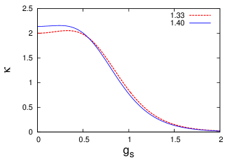
Figure 8: (color online). Flexible model: The elastic modulus as a function of $g_{s}$ at $y=4/3=y_{c}$ [Eq. (16] and $y=1.40>y_{c}$ [from Eqs. (9a) and (9b)].

Finite-length DNA.

The contribution of the bubbles becomes significant in finite-length DNA as shown in Fig. 6. The finite-size effects become significant when the length is comparable to or shorter than the length of the bubble fluctuations. The elastic constant for a finite-length DNA is necessarily continuous, devoid of any singularity, but it should evolve into a discontinuous function as the length is increased. This indicates that shorter chains will show a larger deviation from the thermodynamic limit over a range of forces. A finite-size scaling form is

$$\kappa={\sf f}((g_{s}-g_{sc})N^{1/\nu}),$$ (17)

so that $\kappa={\sf f}(0)$ at $g_{s}=g_{sc}$ for all finite $N$. Therefore all the finite-size curves pass through a common point as shown in Fig. 6, which is the critical point. By identifying the common points for other $y$ values we can now determine the phase diagram numerically. This is shown in Fig. 2. The consistency between this numerical method of finding the critical points with the analytical results helps us when the model under consideration is not solvable analytically. All the points in this phase boundary including the thermal melting point $(y=4/3,g_{sc}=0)$ are second-order critical points. The behavior of $\kappa$ shows that the system is most flexible when it is in the unbound state and under no external force, as it has the highest value of $\kappa$.

III.3 Role of the bubbles

To highlight the importance of the bubbles we compare our results with the Y-model which is similar to the flexible model except that bubble formation is not allowed there marenduzzo . The bound state of this model is the same as the completely bound state of the flexible model and it has a zero-force melting point (a first-order transition) at $y_{c}=$2. In the presence of $g_{s}$ the corresponding singularities and elastic constants are given by

$$z_{b} = \frac{1}{2y\cosh 2g_{s}},\quad\kappa_{b}=4\ \text{sech}^{2}(2g_{s}),\hskip 2.84544pt\text{and}$$ (18a)

$$z_{f} = \frac{1}{2\cosh^{2}g_{s}},\quad\kappa_{f}=2\ \text{sech}^{2}(g_{s}),$$ (18b)

where $\kappa_{b}$ and $\kappa_{f}$ are the bound-state and the unbound-state elastic constants, respectively. We obtain the phase boundary by equating $z_{b}$ with $z_{f}$ as

$$g_{sc}=\frac{1}{2}\cosh^{-1}\left(\frac{1}{y-1}\right).$$ (19)

The phase boundary has similar asymptotics for $y\to y_{c}(=2)$ and $y\to 1$ as in Eqs. (12a) and (12b). In Fig. 5 we compare $\kappa_{b}$ with the flexible model results. It shows that the flexibility of the bound state of the flexible model is mostly due to the bubbles.

III.4 Elastic response in the presence of an unzipping force

It is well known that this model undergoes an unzipping transition under the influence of an unzipping force in the absence of a stretching force. This unzipping transition is known to be a first-order phase transition. The unzipped state consists of two completely separated independent single strands. When DNA is in the double-stranded form the unzipping force tries to unzip it into two single strands. On the other hand, when DNA is in the unzipped state the stretching force tries to make them bound. Now, if we apply both the forces simultaneously we expect a competition between the opposing effects. In this section we study this problem, again, analytically for the infinite system and numerically for finite systems. We use the same definitions of quantities as in Eqs. (4a), (4b), and (5).

Let us apply a spatially independent unzipping force $g_{u}$ at the rear end of the DNA, i.e., the forces act exactly in opposite directions. In the presence of a stretching force $g_{s}$ the generating function is given by $G(g_{s},z)=A(g_{s},z)\lambda(g_{s},z)^{(x_{1}-x_{2})/2}e^{g_{s}(x_{1}+x_{2})}$, where $A(g_{s},z)$ and $\lambda(g_{s},z)$ are given by Eq. (30a) and Eq. (30b). The generating function in the presence of both forces is given by

$${\cal G}(g_{s},g_{u},z)=\sum_{x_{1},x_{2}}G(g_{s},z)e^{g_{u}(x_{1}-x_{2})}.$$ (20)

So, the bound-state singularity remains the same as $z_{b}$, Eq. (9a), consistent with the hypothesis of non-penetration of forces in the bound state poulomi , but the unbound-state singularity is now given by the solution of the equation $e^{2g_{u}}=\lambda(g_{s},z)$. This equation is easily obtained by performing the summation over $x_{1}$ and $x_{2}$ in Eq. (20). Solving this equation for $z$ we find that the unbound-state singularity $z_{fu}$ is given by

$$z_{fu}=\frac{1}{2\left[\cosh(2g_{s})+\cosh(2g_{u})\right]},$$ (21)

which corresponds to the partition function of the two chains under forces $g_{s}+g_{u}$ and $g_{s}-g_{u}$, namely, $4\cosh(g_{s}+g_{u})\cosh(g_{s}-g_{u})$. For $g_{u}=0$, the corresponding singularity matches Eq. (9b). The transition, as before, is given by the crossing of the singularities at

$$g_{uc}=\frac{1}{2}\cosh^{-1}\left(\frac{1}{2z_{b}}-\cosh\left(2g_{\text{s}}\right)\right).$$ (22)

This expression reduces to the known unzipping line marenduzzo for $g_{s}=0$ and Eq. (11) for $g_{u}=0$.

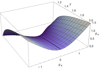
Figure 9: (color online). Flexible model: Three dimensional phase diagram of the system, Eq. (22), in the presence of both stretching and unzipping forces. All points on the surface except the curve for $g_{uc}=0$ represent first-order phase transition points. The unzipping line for $g_{s}=0$ is shown by the thick black line.

III.4.1 Complete phase diagram with unzipping force

After the introduction of an unzipping force we now have three control parameters. By changing any one of them while keeping the other two fixed, one can induce a phase transition in the system. The transition points are distributed on a surface in the $y$-$g_{s}$-$g_{u}$ space given by Eq. (22). In Fig. 9 we plot this function. The critical curve for $g_{uc}=0$ in the surface is a second-order line. Around $g_{s}=0$, $g_{uc}(g_{s})=g_{uc}(0)+ag_{s}^{2}+...$, so that the unzipping line for $g_{s}=0$ lies along the locus of the local minima on the surface. The first-order surface ends on the $g_{u}=0$ plane in a critical line that contains the usual melting point at $y_{c}(g_{s}=g_{u}=0)$. Except for the critical line all the other possible lines on the surface are first-order lines. To show that there is indeed a first-order transition we plot $n_{c}$ as a function of $g_{s}$ in Fig. 3 with $g_{u}>0$ and $y$ kept fixed.

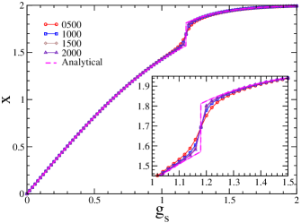
Figure 10: (color online). Flexible model: $x$ vs $g_{s}$ plot, with $g_{u}=0.4$ and $y=1.20$. Inset: Magnification of the critical region. The dotted magenta line is the analytical curve. See Sec. III.4.2. All other curves are for finite system sizes shown in the legend. The discontinuity at $g_{sc}$ indicates a first order transition. Solid lines through the data points are guides for the eye.

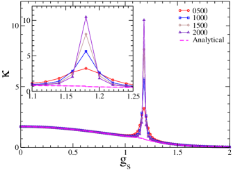
Figure 11: (color online). Flexible model: $\kappa$ vs $g_{s}$ plot with $g_{u}=0.4$ and $y=1.20$. Inset: Magnification of the critical region. The dotted magenta lines are the analytical curves. See Sec. III.4.2. All other curves are for finite system sizes shown in the legend. The peak height increases proportionally with $N$, signaling a $\delta$-function peak which is not shown in the analytical curve. Solid lines through the data points are guides for the eye.

III.4.2 Elastic constant

We plot $x$ vs $g_{s}$ in Fig. 10 and $\kappa$ vs $g_{s}$ in Fig. 11, keeping $g_{u}$ and $y$ at fixed values. The dotted magenta curves are the analytical ones for an infinite system length, obtained by using Eqs. (3), (9a), and (21), while all the other curves are for finite system sizes which gradually match the analytical curve as $N$ becomes larger. $x$ shows a finite discontinuity at a critical $g_{sc}=1.18$. The analytical curve for $\kappa$ has a $\delta$-function peak at $g_{sc}$, which is not shown in Fig. 11. The uniform increase in the peak height with increasing system size in $\kappa$ at the critical point is the signature of the delta peak. Below we list various useful limiting values of $x$ and $\kappa$.

1. $\text{For}\quad g_{s}\to 0,g_{u}>g_{uc}(y)$,

   $$x \approx 2\ \text{sech}^{2}\left(g_{u}\right)g_{s},$$ (23a)

   $$\kappa \approx 2\ \text{sech}^{2}\left(g_{u}\right)+2\frac{\cosh(g_{u})-2}{\cosh^{4}(g_{u})}g_{s}^{2}.$$ (23b)

2. $\text{For}\quad g_{s}\to 0,g_{u}<g_{uc}(y),$

   $$x \approx 4\sqrt{\frac{y-1}{y}}g_{s},$$ (24a)

   $$\kappa \approx 4\sqrt{\frac{y-1}{y}}+\frac{8(3-2y)\sqrt{y-1}}{y^{3/2}}g_{s}^{2}.$$ (24b)

3. $\text{For}\quad g_{s}\to g_{sc}-,y=1.2,g_{u}=0.4$,

   $$x \approx 1.57107+0.73049(g_{s}-g_{sc}),$$ (25a)

   $$\kappa \approx 0.73049-1.03646(g_{s}-g_{sc}).$$ (25b)

4. $\text{For}\quad g_{s}\to g_{sc}+,y=1.2,g_{u}=0.4$,

   $$x \approx 1.81211+0.66067(g_{s}-g_{sc}),$$ (26a)

   $$\kappa \approx 0.66067-2.01486(g_{s}-g_{sc}).$$ (26b)

For an infinite system the transition occurs suddenly at a single point. On the other hand, for a finite-size system the effect of the transition remains relevant for a domain of $g_{s}$ values containing $g_{sc}$ beyond the scaling regime.

IV Rigid Model

Here we customize the previous model to incorporate explicit weights for bubble formation. Doing that in the transfer matrix format is a bit involved. To identify a bubble we need to ensure that an unbound region is attached between two bound segments. A bound segment is defined as a DNA patch where every base pair is in the bound state and the minimum length it can have is 2. We implement this by applying the constraint that a bound base pair can form only if another bound base-pair precedes it. So, for every step in the generation of the polymers we need to keep track of the previous step. We introduce a built-in rigidity to the dsDNA by instituting a bias against the bending towards the right of bound segments. For computational simplicity here we completely switch off the rightward option. By doing this we are introducing a bias in the propagation of DNA in favor of one direction. Other than the usual contact weight $y$ we introduce another Boltzmann weight $v$ if a bound segment opens to form two single strands or two single strands recombine to form a bound segment. The recursion relation which obeys these rules is given by

$$z_{n}(x_{1},x_{2})=\\ \begin{cases}\text{\color[rgb]{0,0,1}y}[\text{\color[rgb]{1,0,0}v}z_{n-1}(i,l)+\text{\color[rgb]{1,0,0}v}z_{n-1}(j,k)+z_{n-1}(j,l)],&\text{if}\hskip 7.22743ptx_{1}=x_{2}\&n>0\\ \text{\color[rgb]{1,0,0}v}z_{n-1}(i,l)+z_{n-1}(i,k)+z_{n-1}(j,k)+z_{n-1}(j,l),&\text{if}\hskip 7.22743ptx_{1}-x_{2}=2\&n=1\\ \text{\color[rgb]{1,0,0}v}z_{n-1}(j,k)+z_{n-1}(i,k)+z_{n-1}(i,l)+z_{n-1}(j,l),&\text{if}\hskip 7.22743ptx_{1}-x_{2}=-2\&n=1\\ \text{\color[rgb]{1,0,0}v}\text{\color[rgb]{0,0,1}y}z_{\text{\color[rgb]{1,0,0}n-2}}(i+1,l+1)+z_{n-1}(i,k)+z_{n-1}(j,k)+z_{n-1}(j,l),&\text{if}\hskip 7.22743ptx_{1}-x_{2}=2\&n\geq 2\\ \text{\color[rgb]{1,0,0}v}\text{\color[rgb]{0,0,1}y}z_{\text{\color[rgb]{1,0,0}n-2}}(j+1,k+1)+z_{n-1}(i,l)+z_{n-1}(i,k)+z_{n-1}(j,l),&\text{if}\hskip 7.22743ptx_{1}-x_{2}=-2\&n\geq 2\\ z_{n-1}(i,k)+z_{n-1}(i,l)+z_{n-1}(j,k)+z_{n-1}(j,l),&\text{if}\hskip 7.22743pt\left|x_{1}-x_{2}\right|>2\&n>0\end{cases},$$ (27)

with $i=x_{1}-1$, $j=x_{1}+1$, $k=x_{2}-1$ and $l=x_{2}+1$. The first two steps fix the initial configurations. To fix the configuration at the $n$th step we need to keep the information on not only the $(n-1)$th step but also the $(n-2)$th step. We evaluate the recursion relation, Eq. (27), exactly for finite system sizes by iterating it numerically. Once $Z(x_{1},x_{2})$ is known, the force-dependent partition function can be obtained with the help of Eq. (2), and the corresponding elastic constant from Eq. (3). Only the stretching force $g_{s}$ is considered here. Using the bubble weight $v$ we can now count the average number of bubbles $(n_{b})$ and calculate the average bubble length $(l_{b})$. They are formally given by the formulas

$$n_{b}=\frac{v^{2}}{N}\frac{\partial f}{\partial v^{2}},\hskip 2.84544ptC_{b}=v^{2}\frac{\partial n_{b}}{\partial v^{2}}\hskip 2.84544pt,\text{and}\hskip 2.84544ptl_{b}=\frac{(1-n_{c})}{n_{b}},$$ (28)

where $C_{b}$ describes the fluctuations in $n_{b}$. To evaluate them numerically, first we take the first and second derivatives of Eq. (27) with respect to $v$ and iterate them numerically by setting $v=1$ to obtain the first and the second derivatives of the zero-force partition function respectively. Once the derivatives of the partition function are known, $n_{b}$, $C_{b}$, and $l_{b}$ can be determined by using Eq. (28) for a zero applied force. To find out the corresponding quantities for nonzero constant forces and to find out $n_{c}$ and $C_{c}$, we follow the method described in Section III.1.

IV.1 Thermal Melting : $g_{s}=0$

First, let us show that this model goes through a binding-unbinding transition as $y$ is varied in the absence of any external forces. For the analysis in this section we set $v=1$. Here we use the exact numerical transfer matrix method for finite-size systems.

In Fig. 12 we show how the average number of contacts varies with $y$. As the system size is increased one part of the curve gradually touches the $y$ axis. And it is also evident that $n_{c}$ will saturate at $n_{c}=1$ for appropriately high $y$ values. These indicate a binding-unbinding transition. To find out the order of the transition and the corresponding critical value of $y$, $y_{c}$, we plot $C_{c}$ vs $y$ in Fig. 13. $C_{c}$ obeys a finite size scaling relation similar to Eq. (17) which indicates a finite discontinuity. At $y=1.18$ all the curves pass through a common point, implying $y_{c}=1.18$. The finite discontinuity at $y_{c}$ establishes that this is a second-order phase transition.

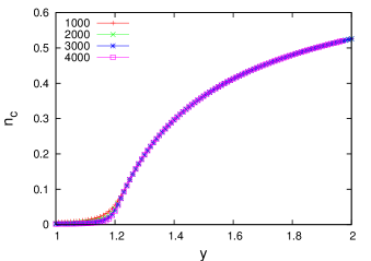
Figure 12: (color online). Rigid model: $n_{c}$ increases from zero to non-zero values continuously at $y>1$ before approaching the saturation value, 1. This indicates a binding-unbinding transition. Solid lines through the data points are guides for the eye.

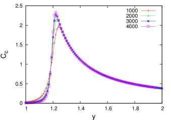
Figure 13: (color online). Rigid model: $C_{c}$ vs $y$ plots for different $N$. The peak height increases with increasing $N$ but eventually saturates, creating a finite discontinuity. The discontinuity occurs at $y=1.18$, where all the curves meet. Solid lines through the data points are guides for the eye.

Note that we have not imposed the non-crossing constraint here. The restriction imposed on the bound state is sufficient to induce a bound-unbound transition. In one spatial dimension the entropy of a system dominates over binding energy, which implies that there is no ordering here. Imposition of special restrictions to limit the entropy may result in an energy dominated ordered state. The non-crossing constraint in the previous model did exactly that by decreasing the total number of configurations. The restriction imposed here on the degrees of freedom of the bound segment plays a similar role, decreasing the total number of configurations of the DNA. We elaborate on this in Appendix B.

IV.2 Elastic response : $g_{s}\neq 0$

Let us now discuss the elastic properties of this system. As discussed earlier the inherent asymmetry in this model favors extension of DNA in one direction and opposes it in the other direction. So under the influence of a spatially independent stretching force the DNA is more flexible in one direction compared to the other direction.

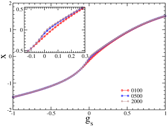
Figure 14: (color online). Rigid model: Continuous stretching of the DNA to its full extent by both positive and negative forces. The $y$ value is fixed at 1.20. Solid lines through the data points are guides for the eye.

Figure 15: (color online). Rigid model: $\kappa$ shows an increasing peak around $g_{s}=0.02$ with increasing system length $N$ and a fixed $y=1.20$. Inset: Maximum values of $\kappa$, $\kappa_{\text{max}}$, are plotted vs $1/N$. A linear fit with the fist four points (solid blue line) gives the estimate for $N\to\infty$, $\kappa_{\text{max}}=4.95$. This indicates that there is a finite discontinuity in $\kappa$. The dashed black line is a plot of the function $\kappa=2\ \text{sech}^{2}(g_{s})$, the unbound-state elastic constant. For $g_{s}>0.02$, $\kappa$ matches the unbound-state modulus. Solid lines through the data points are guides for the eye.

As the system is no longer symmetric under $g_{s}\leftrightarrow-g_{s}$ we need to focus attention on the negative values of $g_{s}$ too. Figure 14 shows that $x$ varies continuously with $g_{s}$, reaching $\pm 2$ for a large positive or negative $g_{s}$. In Fig. 15 we plot $\kappa$ vs $g_{s}$ keeping $y$ fixed. Every curve shows a peak around $g_{s}=0.02$ which increases in height as $N$ increases. The maximum of $\kappa$, $\kappa_{\text{max}}$, goes to a finite value in the $N\to\infty$ limit as shown in the inset in Fig. 15. The inset in Fig. 16 shows how $n_{c}$ changes as we increase $g_{s}$ for $y=1.20$. This indicates a continuous binding-unbinding phase transition. Figure 16 shows that $C_{c}$ has a finite jump at $g_{sc}=0.02$ which can be identified as the common point in the peak region through which every finite-size curve passes. For $g_{s}<g_{sc}$, $\kappa$ shows anomalous behavior, as close to the transition point it can reach values which are much greater than the entropic elastic modulus of the unbound state given by $2\ \text{sech}^{2}(g_{s})$, shown in Fig. 15 as a dashed black line.

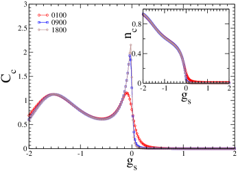
Figure 16: (color online). Rigid model: $C_{c}$ vs $g_{s}$ curves for finite lengths as indicated. The $y$ value is fixed at 1.20. Inset: $n_{c}$ decreases continuously from a finite value to 0, indicating a continuous phase transition. Peak heights in $C_{c}$ vs $g_{s}$ curves saturate, indicating a finite discontinuity. Around $g_{s}=0.02$ all curves meet at the critical point. Solid lines through the data points are guides for the eye.

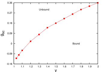
Figure 17: (color online) Rigid model: Numerical phase diagram for the binding-unbinding transition. The solid line through the data points is guide for the eye.

By collecting similar common points for different $y$ values we draw the numerical phase diagram of the system, which is shown in Fig. 17. Noticeable there is that the stretching force actually unbinds the bound state for $g_{s}>g_{sc}$. The reason for this is the following. Due to the bias the bound-state formation on the positive $x$ axis is unfavorable and the DNA prefers to go in the negative $x$ direction. As $g_{s}$ is increased it wins over the bias eventually and pulls the DNA towards the positive $x$ direction. Because the bound state is forbidden in that direction the bound DNA unzips as a result.

IV.3 Role of the bubbles

The flexibility of the bound state comes solely from the bubbles, as the bound segments are absolutely rigid in this model.

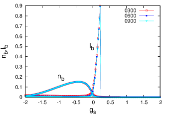
Figure 18: (color online). Rigid model: $n_{b}$ vs $g_{s}$ and $l_{b}$ vs $g_{s}$ plot for $y=1.20$. As the critical point is approached, $n_{b}$ becomes very small but $l_{b}$ becomes as large as $N$. Solid lines through the data points are guides for the eye.

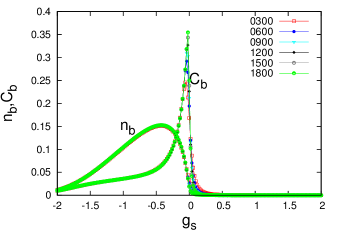
Figure 19: (color online). Rigid model: $n_{b}$ vs $g_{s}$ and $C_{b}$ vs $g_{s}$ plot for $y=1.20$. Around the critical point $n_{b}$ is very small but its fluctuation $C_{b}$ is very large. Solid lines through the data points are guides for the eye.

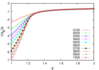
Figure 20: (color online). Rigid model: $\frac{1}{x}\sqrt{n_{b}}$ vs $y$ curves for different system lengths collapse to a single master curve in the bound region. $g_{u}=g_{s}=0$. $y_{c}=1.18$. Solid lines through the data points are guides for the eye.

Figure 21: (color online). Rigid model: $\frac{1}{\kappa}\sqrt{C_{b}}$ vs $y$ curves for different system lengths collapse to a single master curve in the bound region. $g_{u}=g_{s}=0$. $y_{c}=1.18$. Solid lines through the data points are guides for the eye.

Figure 18 shows that $n_{b}$ becomes very small while $l_{b}$ increases to almost equal to $N$ as we approach the transition point. Here $l_{b}\approx(N\ \text{or}\ 0)$ means the DNA is in the unzipped state. The peaks in $n_{b}$ curves indicate a large number of bubbles but at the same time of very small average length. From these two observations we can now say that as we approach the transition point many small bubbles coalesce to form large bubbles with decreasing numbers, and eventually $n_{b}$ becomes 0 when the two strands get completely separated. The fluctuation in $n_{b}$, $C_{b}$, also becomes large around the critical point as shown in Fig. 19. Earlier we have shown that $\kappa$ in this model behaves anomalously and the anomalous behavior occurs in the same region where $l_{b}$ and $C_{b}$ are the largest. In our model, $\kappa$ is the fluctuation of extension $x$ by definition and it depends on $n_{b}$. For example, near the transition point $n_{b}$ is very small and $x$ is also very small, although $l_{b}$ is large. This is because in the $(1+1)$ dimension $x$ for a single strand is 0 due to its Gaussian nature. But for a bound DNA, $x\propto\sqrt{n_{b}}$ as shown in Fig. 20. It is then expected that $\kappa$ will be determined by the fluctuations in $n_{b}$, $C_{b}$. In Fig. 21 we plot $\frac{1}{\kappa}\sqrt{C_{b}}$ vs $y$ for different system sizes in the absence of any external force. For the bound region $(y>1.18)$ the curves collapse into a single master curve which is almost $y$ independent, inferring that

$$\kappa\approx 7.7\sqrt{C_{b}}.$$ (29)

We therefore conclude that $C_{b}$ is the important factor in determining the elastic behavior of the system.

V Discussion And Summary

There are a few points which we feel need to be clarified in more detail. (a) As the free ends of the two strands are stretched more and more with increasing forces in the same direction, they are bound to come closer due to their equal lengths and the starting ends’ being attached to each other. This coming closer together increases the possibility of the strands’ forming a bound base pair by gaining energy. (b) The transition in the presence of the unzipping force is definitely an unzipping transition. This is true even if $g_{u}$ is very small. (c) $\kappa$ in the flexible model is sensitive to the changes in $g_{u}$, $g_{s}$, and $y$. Elasticity is entropic in nature, which emerges from collective behavior. The rigid model, on the other hand, has its own intrinsic elasticity. This is reflected in the anomalous behavior of $\kappa$ for this model. (d) The single-molecule DNA experimental setup in which stretching force is achieved by placing the DNA in a directional flow can be a testing platform of our models. (e) In the nanopore sequencing technique, dsDNA is unzipped and a single strand is passed through a nanopore nanopore . Other than that, during bacterial conjugation or infection of a cell by a virus the DNA assumes similar geometry. Our study may be relevant in these cases. (f) Single molecule DNA unzipping experiments are normally done at room temperature. In Eq. (22) we provided a phase boundary which depends not only on the temperature and the unzipping force, but also on the stretching force. Its remains a challenge to generate this phase boundary experimentally with temperature as a variable in single-molecule experiments.

We summarize the basic results on rigidity as defined by Eq. (3) for the two models.

For the entropic rigidity as seen in the flexible-chain model of DNA, we obtained the following exact results. (1) For $g_{s}=g_{u}=0$,

$$\kappa(g_{s}=0)=\begin{cases}2,&\text{for}\quad y<y_{c},\\ 4\sqrt{\frac{y-1}{y}},&\text{for}\quad y>y_{c},\end{cases}$$

(2) For $y=y_{c}$, i.e. at the critical point,

$$\kappa(y=y_{c})=\frac{64w\left(w+1\right)}{\left(w^{2}+14w+1\right)^{3/2}},\ \text{with}\quad w=e^{4g_{s}}.$$

In the presence of the two opposing forces, $g_{s}$ as the stretching force and $g_{u}$ as the unzipping force, the transition surface in the $y$-$g_{s}$-$g_{u}$ space is given by Eq. (22).

For the model with intrinsic rigidity, the main result we obtained is

$$\kappa\approx 7.7\sqrt{C_{b}}.$$

VI Conclusion

We have studied the effect of melting of DNA on its elasticity using $(1+1)$ dimensional models by employing exact numerical and analytical methods. Under a stretching force DNA goes through a second-order binding-unbinding phase transition. The dependence of DNA flexibility on the stretching force, the unzipping force, and the temperature has also been discussed. In the presence of both forces the system goes through a first-order unzipping transition. The complete phase diagram in the $y$-$g_{s}$-$g_{u}$ space is obtained. The average bubble length and the average bubble number for our model for different parameter values are also studied. We have shown that the DNA flexibility is related to the bubble number fluctuations. For zero external forces, the extension of the DNA is temperature independent and varies with the square root of the bubble numbers proportionally, while the elastic modulus is also proportional to the square root of the bubble number fluctuation. Though the binding-unbinding transition is very sharp for an infinite-length system, the transition point can influence the elastic behavior of DNA for a broad region of parameter values when the system length is finite. Consequently, the elastic response of short-length DNA, as used extensively in experiments, has to be widely different from that of long-chain DNA. Furthermore, though DNA is a very long molecule, it can melt locally, depending on the environment it is in. Thus our study will help us to understand the importance of these locally melted regions of shorter lengths in determining the elastic properties of the DNA as a whole.

Appendix A $A(g_{s},z)$ AND $\lambda(g_{s},z)$

Forms of $A(g_{s},z)$ and $\lambda(g_{s},z)$ needed for $z_{b}$ and $z_{f}$ (Eqs. (9a) (9b)) are given by

$$A(g_{s},z) = \frac{-1/(2z)}{\cosh(2g_{s})-\sqrt{\left(\cosh(2g_{s})-\frac{1}{2z}\right)^{2}-1}+\frac{(y-2)}{2yz}},$$ (30a)

$$\lambda(g_{s},z) = \sqrt{\left(\cosh(2g_{s})-\frac{1}{2z}\right)^{2}-1}+\frac{1}{2z}-\cosh(2g_{s}).$$ (30b)

Appendix B BIAS-INDUCED MELTING

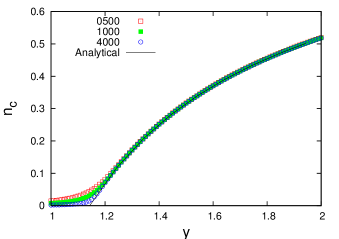
Figure 22: (color online). $n_{c}$ vs $y$ plot for $b=0.5$. $n_{c}$ becomes finite at $y=1.142$. Numerical data are also consistent with the analytical result. Solid lines through the data points are guides are the eye.

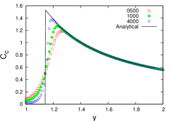
Figure 23: (color online). $C_{c}$ vs $y$ plot for $b=0.5$ showing a finite discontinuity at $y=1.142$. Numerical data also show very similar behavior. Solid lines through the data points are guides for the eye.

In the rigid model we have completely switched off one degree of freedom for the bound segments. We can do the entropy limiting job in a more general way by introducing a control parameter $b$ instead, such that for $b=0$ we block a degree of freedom of the bound state completely, for $b=1$ we get back the good old free Gaussian chain, and for the intermediate values of $b$ we obtain a partially biased scenario. The recursion relation followed by the system is now given by

$$Z_{n+1}(x_{1},x_{1}) = y[Z_{n}(x_{1}+1,x_{1}+1)+Z_{n}(x_{1}+1,x_{1}-1)$$

$$+Z_{n}(x_{1}-1,x_{1}+1)+bZ_{n}(x_{1}-1,x_{1}-1)],$$

$$Z_{n+1}(x_{1},x_{2}) = [Z_{n}(x_{1}+1,x_{2}+1)+Z_{n}(x_{1}+1,x_{2}-1)$$ (31)

$$+Z_{n}(x_{1}-1,x_{2}+1)+Z_{n}(x_{1}-1,x_{2}-1)]$$

$$\text{for}\hskip 5.69046ptx_{1}\neq x_{2},$$

where $Z_{n}(x_{1},x_{2})$ is the partition function for the system length $n$. We set the initial condition as $Z_{0}(0,0)=y$ such that two strands start from the origin. The microscopic parameter $b$ is a Boltzmann weight which controls the possibility of the two polymers’ both going to the right-hand side while being in the bound state. All the notations and definitions of the observables which are used in this model are the same as for the flexible model. By $z$-transforming Eq. (B) using the initial condition we get two independent equations for $x_{1}\neq x_{2}\neq 0$ and $x_{1}=x_{2}=0$:

$$\frac{1}{z}G(z,x_{1},x_{2}) = G(z,x_{1}+1,x_{2}+1)+G(z,x_{1}-1,x_{2}+1)$$ (32a)

$$+G(z,x_{1}+1,x_{2}-1)$$

$$+G(z,x_{1}-1,x_{2}-1),$$

$$\frac{1}{yz}G(z,0,0) = \frac{1}{z}+G(z,1,1)+G(z,-1,1)$$ (32b)

$$+G(z,1,-1)+bG(z,-1,-1).$$

To solve these independent equations we make an ansatz for the generating function, $G(z,x_{1},x_{2})=A(z)\lambda(z)^{\text{Abs}[(x_{1}-x_{2})/2]}$. Substituting this ansatz in Eq. (32a) and Eq. (32b) and solving for $A$ and $\lambda$ we get

$$A = \frac{1}{-bz+\frac{1}{y}+z+\sqrt{1-4z}-1},$$ (33a)

$$\lambda = -\frac{2z+\sqrt{1-4z}-1}{2z}.$$ (33b)

The bound-state and unbound-state singularities are given by

$$z_{b} = \frac{b-1-y(b+1)+\sqrt{y}\sqrt{(b+1)^{2}y-4b+4}}{(b-1)^{2}y},$$ (34a)

$$z_{f} = \frac{1}{4}.$$ (34b)

From these singularities all the other relevant quantities can be derived. Figure 22 shows how $n_{c}$ varies with $y$. At a high enough $y$, $n_{c}$ saturates to its maximum value, 1. In Fig. 23 we plot $C_{c}$ vs $y$. In both Fig. 22 and Fig. 23 we also show the corresponding numerical data for different finite system sizes. $C_{c}$ obeys a finite-size scaling form $C_{c}=g((y-y_{c})N^{1/\delta})$ such that at $y=y_{c}=1.142$, $C_{c}(y_{c})=g(0)$. The numerical data are consistent with the analytical results. From these two figures we conclude that the system is going through the usual second-order binding-unbinding phase transition. We obtain the critical point of this transition analytically by matching $z_{b}$ with $z_{f}$. The critical value of $y$ is now $b$ dependent and varies with $b$ as $y_{c}=4/(3+b)$. For $b=1$ we have the same recursion relation as that of a system with two Gaussian chains which can freely cross each other and in which there is no phase transition. In our case also we get $y_{c}=1$, which means that there is no phase transition at finite temperature. Another interesting limit is when $b=0$, $y_{c}=4/3$, the critical point for two Gaussian chains with noncrossing constraint, although the recursion relations for these two cases are not the same. Moreover, the $b$ dependence of $y_{c}$ in our model adds extra flexibility in that we can now tune the critical point by tuning $b$ for a wide range of values.

From the recursion relation it is clear that the parameter $b$ just modulates one of the four possible contributions to the partition function of the $n$th generation from the $(n-1)$th generation. $b$ may be associated with any of the four possible contributions. The case when $b$ is attached to the $z(x_{1}-1,x_{2}+1)$ term is of special interest because the $b\rightarrow 0$ limit is exactly the flexible noncrossing case now. This current case also is exactly solvable through the generating function technique and gives exactly the same $b$-dependent critical melting point, $y_{c}=4/(3+b)$. So, we can now actually modulate the noncrossing constraint through $b$ and the corresponding critical point as well.

References

- (1) K. Zahn and F.R. Blattner, Science 236, 416(1987).
- (2) J. Kim, C. Zwieb, C. Wu and S. Adhya, Gene 85, 15(1989).
- (3) K. Giese, J. Cox and R. Grosschedl, Cell 69, 185 (1992).
- (4) S. C. Schultz, G. C. Shields and T. A. Steitz, Science 253, 1001 (1991).
- (5) A. K. Nagaich, E. Appella and E. R. Huttington, J. Biol. Chem. 272, 14842 (1997).
- (6) M. E. Ortega and C. E. Catalano, Biochemistry 45, 5180 (2006).
- (7) J. D. Watson, Molecular Biology of the Gene, 7th ed. (Pearson, Cold Spring Harbor, NY, 2013).
- (8) S. Oehler, M. Amouyal, P. Kolkhof, B. Wilcken-Bergmann, and B. Muller-Hill, EMBO J. 13, 3348 (1994).
- (9) T. J. Richmond and C. A. Davey, Nature (London) 423, 145 (2003).
- (10) A. Vologodskii, Biophysics of DNA, (Cambridge University Press, Cambridge, 2015).
- (11) M. Doi and S. F. Edwards, The Theory of Polymer Dynamics (Oxford University Press, Oxford, 1986).
- (12) S. M. Bhattacharjee, A. Giacometti and A. Maritan, J. Phys.: C ondens. Matter 25, 503101 (2013).
- (13) T. E. Cloutier and J. Widom, PNAS 102, 3645 (2005).
- (14) P. A. Wiggins, T.V. D. Heijden, F. Moreno-Herrero, A. Spakowitz, R. Phillips, J. Widom, C. Dekker, and P. C. Nelson, Nat. Nanotechnol. 1, 137 (2006).
- (15) J. Yan and J. F. Marko, Phys. Rev. Lett. 93, 108108 (2004).
- (16) P. Ranjith, P.B. Sunil Kumar and G. Menon, Phys. Rev. Lett. 94, 138102 (2005)
- (17) R. Padinhateeri, G. I. Menon, Biophys. J. 104, 463 (2013).
- (18) Q. Du, C. Smith, N. Shiffeldrim, M. Vologodskaia and A. Vologodskii, PNAS 102, 5397 (2005).
- (19) A. K. Mazur, Phys. Rev. Lett. 98, 218102 (2007).
- (20) A. Noy, R. Golestanian, Phys. Rev. Lett. 109, 228101 (2012).
- (21) R. P. Linna, K. Kaski, Phys. Rev. Lett. 100, 168104 (2008).
- (22) H. Shroff, D. Sivak, J. J. Siegel, A. L. McEvoy, M. Siu, A. Spakowitz, P. L. Geissler, and J. Liphardt, Biophys. J. 94, 2179 (2008).
- (23) R. A. Forties, R. Bundschuh, and M. G. Poirier, Nucleic Acids Res. 37, 4580 (2009).
- (24) T.T. Le and H. D. Kim, Nucleic Acids Res. 42, 10786 (2014).
- (25) A. Vologodskii and M. D. Frank-kramenetskii, Nucleic Acids Res. 41, 6785 (2013).
- (26) J. Ramstein and R. Lavery, PNAS 85, 7231 (1988).
- (27) J. Maji, S. M. Bhattacharjee, F. Seno and A. Trovato New J. Phys. 12, 083057 (2010).
- (28) J. Maji and S. M. Bhattacharjee Phys. Rev. E 86, 041147 (2012).
- (29) J. Maji, S. M. Bhattacharjee, F. Seno and A. Trovato, Phys Rev E 89, 012121 (2014).
- (30) T. Pal, P. Sadhukhan, and S. M. Bhattacharjee, Phys. Rev. Lett. 110, 028105 (2013).
- (31) T. Pal, P. Sadhukhan, and S. M. Bhattacharjee, Phys. Rev. E 91, 042105 (2015).
- (32) D. Poland and H. Scheraga, J. Chem. Phys. 45, 1456 (1966).
- (33) M. Peyrard and A. R. Bishop, Phys. Rev. Lett. 62, 2755 (1989).
- (34) T. Dauxois, M. Peyrard and A. R. Bishop, Physica. D 66, 35 (1993).
- (35) M. Perard, Nonlinearity 17, R1 (2004).
- (36) M. D. Frank-Kamenetskii and S. Prakash, Phys. Life Rev. 11, 153 (2014).
- (37) Y. Kafri, D. Mukamel and L. Peliti, Phys. Rev. Lett. 85, 4988 (2000).
- (38) Y. Kafri, D. Mukamel and L. Peliti, Eur. Phys. J. B 27, 132 (2002).
- (39) D. Marenduzzo, A. Trovato, and A. Maritan, Phys. Rev. E 64, 031901 (2001).
- (40) D. Marenduzzo, S. M. Bhattacharjee, A. Maritan and E. Orlandini, Phy. Rev. Lett. 88, 028102 (2002).
- (41) M. Ya. Azbel, Phys. Rev. E 20, 1671 (1979).
- (42) P. Sadhukhan and S. M. Bhattacharjee, Ind. J. Phys. 88, 895 (2014).
- (43) M. E. Fisher, J. Chem. Phys. 45, 1469 (1966).
- (44) S. Mukherjee and S. M. Bhattacharjee, Phys. Rev. E 63, 051103 (2001).
- (45) S. M. Bhattacharjee, J. Phys. A 33, L423 (2000).
- (46) S Kumar and M S Li, Phys. Rept. 486, 1 (2010).
- (47) M. D. Barkley and B. H. Zimm, J. Chem. Phys. 70, 2991 (1979).
- (48) Y. Seol, J. Li, P. C. Nelson, T. T. Perkins and M. D. Betterton, Biophys. J. 93, 4360 (2007)
- (49) N. Theodorakopoulos and M. Peyrard, Phys. Rev. Lett. 108, 078104 (2012).
- (50) P. A. Wiggins, R. Phillips, and P. C. Nelson, Phys. Rev. E 71, 021909 (2005)
- (51) J. Palmeri, M. Manghi and N. Destainville, Phys. Rev. E 77, 011913 (2008).
- (52) R. Kapri, Phys. Rev. E 90, 062719 (2014).
- (53) R. Kapri, Phys. Rev. E 86, 041906 (2012).
- (54) R. Kapri, S. M. Bhattacharjee and F. Seno, Phys. Rev. Lett. 93, 248102 (2004).
- (55) P. Cluzel, A. Lebrun, C. Heller, R. Lavery, J.-L. Viovy, D. Chatenay, and F. Caron, Science 271, 792 (1996).
- (56) D. Marenduzzo, E. Orlandini, F. Seno and A. Trovato, Phys. Rev. E 81, 051926 (2010).
- (57) A. Ahsan, J. Rudinick and R. Bruinsma, Biophys. J. 74, 132 (1998).
- (58) For the inextensibility of the chains there can not be an S-DNA phase in our model as described in sdna0 ; sdna1 ; sdna2 .
- (59) J. Kasianowicz, E. Brandin, D. Branton, and D. Deamer, Proc. Natl. Acad. Sci. U.S.A. 93, 13770 (1996).