Molding CNNs for text: non-linear, non-consecutive convolutions

Abstract

The success of deep learning often derives from well-chosen operational building blocks. In this work, we revise the temporal convolution operation in CNNs to better adapt it to text processing. Instead of concatenating word representations, we appeal to tensor algebra and use low-rank n-gram tensors to directly exploit interactions between words already at the convolution stage. Moreover, we extend the n-gram convolution to non-consecutive words to recognize patterns with intervening words. Through a combination of low-rank tensors, and pattern weighting, we can efficiently evaluate the resulting convolution operation via dynamic programming. We test the resulting architecture on standard sentiment classification and news categorization tasks. Our model achieves state-of-the-art performance both in terms of accuracy and training speed. For instance, we obtain 51.2% accuracy on the fine-grained sentiment classification task.

1 Introduction

Deep learning methods and convolutional neural networks (CNNs) among them have become de facto top performing techniques across a range of NLP tasks such as sentiment classification, question-answering, and semantic parsing. As methods, they require only limited domain knowledge to reach respectable performance with increasing data and computation, yet permit easy architectural and operational variations so as to fine tune them to specific applications to reach top performance. Indeed, their success is often contingent on specific architectural and operational choices.

CNNs for text applications make use of temporal convolution operators or filters. Similar to image processing, they are applied at multiple resolutions, interspersed with non-linearities and pooling. The convolution operation itself is a linear mapping over “n-gram vectors” obtained by concatenating consecutive word (or character) representations. We argue that this basic building block can be improved in two important respects. First, the power of n-grams derives precisely from multi-way interactions and these are clearly missed (initially) with linear operations on stacked n-gram vectors. Non-linear interactions within a local context have been shown to improve empirical performance in various tasks [Mitchell and Lapata, 2008, Kartsaklis et al., 2012, Socher et al., 2013]. Second, many useful patterns are expressed as non-consecutive phrases, such as semantically close multi-word expressions (e.g.,“not that good”, “not nearly as good”). In typical CNNs, such expressions would have to come together and emerge as useful patterns after several layers of processing.

We propose to use a feature mapping operation based on tensor products instead of linear operations on stacked vectors. This enables us to directly tap into non-linear interactions between adjacent word feature vectors [Socher et al., 2013, Lei et al., 2014]. To offset the accompanying parametric explosion we maintain a low-rank representation of the tensor parameters. Moreover, we show that this feature mapping can be applied to all possible non-consecutive n-grams in the sequence with an exponentially decaying weight depending on the length of the span. Owing to the low rank representation of the tensor, this operation can be performed efficiently in linear time with respect to the sequence length via dynamic programming. Similar to traditional convolution operations, our non-linear feature mapping can be applied successively at multiple levels.

We evaluate the proposed architecture in the context of sentence sentiment classification and news categorization. On the Stanford Sentiment Treebank dataset, our model obtains state-of-the-art performance among a variety of neural networks in terms of both accuracy and training cost. Our model achieves 51.2% accuracy on fine-grained classification and 88.6% on binary classification, outperforming the best published numbers obtained by a deep recursive model [Tai et al., 2015] and a convolutional model [Kim, 2014]. On the Chinese news categorization task, our model achieves 80.0% accuracy, while the closest baseline achieves 79.2%.

2 Related Work

Deep neural networks have recently brought about significant advancements in various natural language processing tasks, such as language modeling [Bengio et al., 2003, Mikolov et al., 2010], sentiment analysis [Socher et al., 2013, Iyyer et al., 2015, Le and Zuidema, 2015], syntactic parsing [Collobert and Weston, 2008, Socher et al., 2011a, Chen and Manning, 2014] and machine translation [Bahdanau et al., 2014, Devlin et al., 2014, Sutskever et al., 2014]. Models applied in these tasks exhibit significant architectural differences, ranging from recurrent neural networks [Mikolov et al., 2010, Kalchbrenner and Blunsom, 2013] to recursive models [Pollack, 1990, Küchler and Goller, 1996], and including convolutional neural nets [Collobert and Weston, 2008, Collobert et al., 2011, Yih et al., 2014, Shen et al., 2014, Kalchbrenner et al., 2014, Zhang and LeCun, 2015].

Our model most closely relates to the latter. Since these models have originally been developed for computer vision [LeCun et al., 1998], their application to NLP tasks introduced a number of modifications. For instance, ?) use the max-over-time pooling operation to aggregate the features over the input sequence. This variant has been successfully applied to semantic parsing [Yih et al., 2014] and information retrieval [Shen et al., 2014, Gao et al., 2014]. ?) instead propose (dynamic) k-max pooling operation for modeling sentences. In addition, ?) combines CNNs of different filter widths and either static or fine-tuned word vectors. In contrast to the traditional CNN models, our method considers non-consecutive n-grams thereby expanding the representation capacity of the model. Moreover, our model captures non-linear interactions within n-gram snippets through the use of tensors, moving beyond direct linear projection operator used in standard CNNs. As our experiments demonstrate these advancements result in improved performance.

3 Background

Let $\mathbf{x}\in\mathbb{R}^{L\times d}$ be the input sequence such as a document or sentence. Here $L$ is the length of the sequence and each $\mathbf{x}_{i}\in\mathbb{R}^{d}$ is a vector representing the $i^{th}$ word. The (consecutive) n-gram vector ending at position $j$ is obtained by simply concatenating the corresponding word vectors

$$v_{j}\ =\ [\mathbf{x}_{j-n+1};\mathbf{x}_{j-n+2};\cdots;\mathbf{x}_{j}]$$

Out-of-index words are simply set to all zeros.

The traditional convolution operator is parameterized by filter matrix $\mathbf{m}\in\mathbb{R}^{nd\times h}$ which can be thought of as $n$ smaller filter matrices applied to each $\mathbf{x}_{i}$ in vector $v_{j}$. The operator maps each n-gram vector $v_{j}$ in the input sequence to $\mathbf{m}^{\top}v_{j}\ \in\ \mathbb{R}^{h}$ so that the input sequence $\mathbf{x}$ is transformed into a sequence of feature representations,

$$\left[\mathbf{m}^{\top}v_{1},\cdots,\mathbf{m}^{\top}v_{L}\right]\quad\in\quad\mathbb{R}^{L\times h}$$

The resulting feature values are often passed through non-linearities such as the hyper-tangent (element-wise) as well as aggregated or reduced by “sum-over” or “max-pooling” operations for later (similar stages) of processing.

The overall architecture can be easily modified by replacing the basic n-gram vectors and the convolution operation with other feature mappings. Indeed, we appeal to tensor algebra to introduce a non-linear feature mapping that operates on non-consecutive n-grams.

4 Model

N-gram tensor

Typical $n-$gram feature mappings where concatenated word vectors are mapped linearly to feature coordinates may be insufficient to directly capture relevant information in the $n-$gram. As a remedy, we replace concatenation with a tensor product. Consider a 3-gram $(\mathbf{x}_{1},\mathbf{x}_{2},\mathbf{x}_{3})$ and the corresponding tensor product $\mathbf{x}_{1}\otimes\mathbf{x}_{2}\otimes\mathbf{x}_{3}$. The tensor product is a 3-way array of coordinate interactions such that each $ijk$ entry of the tensor is given by the product of the corresponding coordinates of the word vectors

$$\left(\mathbf{x}_{1}\otimes\mathbf{x}_{2}\otimes\mathbf{x}_{3}\right)_{ijk}=\mathbf{x}_{1i}\cdot\mathbf{x}_{2j}\cdot\mathbf{x}_{3k}$$

Here $\otimes$ denotes the tensor product operator. The tensor product of a 2-gram analogously gives a two-way array or matrix $\mathbf{x}_{1}\otimes\mathbf{x}_{2}\ \in\ \mathbb{R}^{d\times d}$. The n-gram tensor can be seen as a direct generalization of the typical concatenated vector.

Tensor-based feature mapping

Since each n-gram in the sequence is now expanded into a high-dimensional tensor using tensor products, the set of filters are analogously maintained as high-order tensors. In other words, our filters are linear mappings over the higher dimensional interaction terms rather than the original word coordinates.

Consider again mapping a 3-gram $(\mathbf{x}_{1},\mathbf{x}_{2},\mathbf{x}_{3})$ into a feature representation. Each filter is a 3-way tensor with dimensions $d\times d\times d$. The set of $h$ filters, denoted as $T$, is a 4-way tensor of dimension $d\times d\times d\times h$, where each $d^{3}$ slice of $T$ represents a single filter and $h$ is the number of such filters, i.e., the feature dimension. The resulting $h-$dimensional feature representation $z\in\mathbb{R}^{h}$ for the 3-gram $(\mathbf{x}_{1},\mathbf{x}_{2},\mathbf{x}_{3})$ is obtained by multiplying the filter $\mathbf{T}$ and the 3-gram tensor as follows. The $l^{th}$ coordinate of $z$ is given by

$$z_{l} =\sum_{ijk}\mathbf{T}_{ijkl}\cdot\left(\mathbf{x}_{1}\otimes\mathbf{x}_{2}\otimes\mathbf{x}_{3}\right)_{ijk}$$

$$=\sum_{ijk}\mathbf{T}_{ijkl}\cdot\mathbf{x}_{1i}\cdot\mathbf{x}_{2j}\cdot\mathbf{x}_{3k}$$ (1)

The formula is equivalent to summing over all the third-order polynomial interaction terms where tensor $\mathbf{T}$ stores the coefficients.

Directly maintaining the filters as full tensors leads to parametric explosion. Indeed, the size of the tensor $\mathbf{T}$ (i.e. $h\times d^{n}$) would be too large even for typical low-dimensional word vectors where, e.g., $d=300$. To this end, we assume a low-rank factorization of the tensor $\mathbf{T}$, represented in the Kruskal form. Specifically, $\mathbf{T}$ is decomposed into a sum of $h$ rank-1 tensors

$$\mathbf{T}=\sum_{i=1}^{h}\mathbf{P}_{i}\otimes\mathbf{Q}_{i}\otimes\mathbf{R}_{i}\otimes\mathbf{O}_{i}$$

where $\mathbf{P},\mathbf{Q},\mathbf{R}\in\mathbb{R}^{h\times d}$ and $\mathbf{O}\in\mathbb{R}^{h\times h}$ are four smaller parameter matrices. $\mathbf{P}_{i}$ (similarly $\mathbf{Q}_{i}$, $\mathbf{R}_{i}$ and $\mathbf{O}_{i}$) denotes the $i^{th}$ row of the matrix. Note that, for simplicity, we have assumed that the number of rank-1 components in the decomposition is equal to the feature dimension $h$. Plugging the low-rank factorization into Eq.(1), the feature-mapping can be rewritten in a vector form as

$$z\ =\ \mathbf{O}^{\top}\left(\mathbf{P}\mathbf{x}_{1}\odot\mathbf{Q}\mathbf{x}_{2}\odot\mathbf{R}\mathbf{x}_{3}\right)$$ (2)

where $\odot$ is the element-wise product such that, e.g., $(a\odot b)_{k}=a_{k}\times b_{k}$ for $a,b\in\mathbb{R}^{m}$. Note that while $\mathbf{P}\mathbf{x}_{1}$ (similarly $\mathbf{Q}\mathbf{x}_{2}$ and $\mathbf{R}\mathbf{x}_{3}$) is a linear mapping from each word $\mathbf{x}_{1}$ (similarly $\mathbf{x}_{2}$ and $\mathbf{x}_{3}$) into a $h$-dimensional feature space, higher order terms arise from the element-wise products.

Non-consecutive n-gram features

Traditional convolution uses consecutive n-grams in the feature map. Non-consecutive n-grams may nevertheless be helpful since phrases such as “not good”, “not so good” and “not nearly as good” express similar sentiments but involve variable spacings between the key words. Variable spacings are not effectively captured by fixed n-grams.

We apply the feature-mapping in a weighted manner to all n-grams thereby gaining access to patterns such as “not … good”. Let $z[i,j,k]\in\mathbb{R}^{h}$ denote the feature representation corresponding to a 3-gram $(\mathbf{x}_{i},\mathbf{x}_{j},\mathbf{x}_{k})$ of words in positions $i$, $j$, and $k$ along the sequence. This vector is calculated analogously to Eq.(2),

$$z[i,j,k]\ =\ \mathbf{O}^{\top}\left(\mathbf{P}\mathbf{x}_{i}\odot\mathbf{Q}\mathbf{x}_{j}\odot\mathbf{R}\mathbf{x}_{k}\right)$$

We will aggregate these vectors into an $h-$dimensional feature representation at each position in the sequence. The idea is similar to neural bag-of-words models where the feature representation for a document or sentence is obtained by averaging (or summing) of all the word vectors. In our case, we define the aggregate representation $z_{3}[k]$ in position $k$ as the weighted sum of all 3-gram feature representations ending at position $k$, i.e.,

$$z_{3}[k] =\sum_{i<j<k}z[i,j,k]\cdot\lambda^{(k-j-1)+(j-i-1)}$$

$$=\sum_{i<j<k}z[i,j,k]\cdot\lambda^{k-i-2}$$ (3)

where $\lambda\in[0,1)$ is a decay factor that down-weights 3-grams with longer spans (i.e., 3-grams that skip more in-between words). As $\lambda\rightarrow 0$ all non-consecutive 3-grams are omitted, $z_{3}[k]=z[k-2,k-1,k]$, and the model acts like a traditional model with only consecutive n-grams. When $\lambda>0$, however, $z_{3}[k]$ is a weighted average of many 3-grams with variable spans.

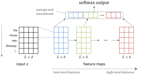
Figure 1: Illustration of the model architecture. The input is represented as a matrix where each row is a d-dimensional word vector. Several feature map layers (as described in Section 4) are stacked, mapping the input into different levels of feature representations. The features are averaged within each layer and then concatenated. Finally a softmax layer is applied to obtain the prediction output.

Aggregating features via dynamic programming

Directly calculating $z_{3}[\cdot]$ according to Eq.(3) by enumerating all 3-grams would require $O(L^{3})$ feature-mapping operations. We can, however, evaluate the features more efficiently by relying on the associative and distributive properties of the feature operation in Eq.(2).

Let $f_{3}[k]$ be a dynamic programming table representing the sum of 3-gram feature representations before multiplying with matrix $\mathbf{O}$. That is, $z_{3}[k]=\mathbf{O}^{\top}f_{3}[k]$ or, equivalently,

$$f_{3}[k] =\sum_{i<j<k}\lambda^{k-i-2}\cdot\left(\mathbf{P}\mathbf{x}_{i}\odot\mathbf{Q}\mathbf{x}_{j}\odot\mathbf{R}\mathbf{x}_{k}\right)$$

We can analogously define $f_{1}[i]$ and $f_{2}[j]$ for 1-grams and 2-grams,

$$f_{1}[i] =\mathbf{P}\mathbf{x}_{i}$$

$$f_{2}[j] =\sum_{i<j}\ \lambda^{j-i-1}\cdot\left(\mathbf{P}\mathbf{x}_{i}\odot\mathbf{Q}\mathbf{x}_{j}\right)$$

These dynamic programming tables can be calculated recursively according to the following formulas:

$$f_{1}[i] =\ \mathbf{P}\mathbf{x}_{i}$$

$$s_{1}[i] =\ \lambda\cdot s_{1}[i-1]+f_{1}[i]\quad\quad\quad$$

$$f_{2}[j] =\ s_{1}[j-1]\odot\mathbf{Q}\mathbf{x}_{j}$$

$$s_{2}[j] =\ \lambda\cdot s_{2}[j-1]+f_{2}[j]$$

$$f_{3}[k] =\ s_{2}[k-1]\odot\mathbf{R}\mathbf{x}_{k}$$

$$z[k] =\mathbf{O}^{\top}\left(f_{1}[k]+f_{2}[k]+f_{3}[k]\right)$$

where $s_{1}[\cdot]$ and $s_{2}[\cdot]$ are two auxiliary tables. The resulting $z[\cdot]$ is the sum of 1, 2, and 3-gram features. We found that aggregating the 1,2 and 3-gram features in this manner works better than using 3-gram features alone. Overall, the n-gram feature aggregation can be performed in $O(Ln)$ matrix multiplication/addition operations, and remains linear in the sequence length.

The overall architecture

The dynamic programming algorithm described above maps the original input sequence to a sequence of feature representations $\mathbf{z}=z[1:L]\in\mathbb{R}^{L\times h}$. As in standard convolutional architectures, the resulting sequence can be used in multiple ways. One can directly aggregate it to a classifier or expose it to non-linear element-wise transformations and use it as an input to another sequence-to-sequence feature mapping.

The simplest strategy (adopted in neural bag-of-words models) would be to average the feature representations and pass the resulting averaged vector directly to a softmax output unit

$$\bar{z} =\frac{1}{L}\sum_{i=1}^{L}z[i]$$

$$\tilde{y} =\text{softmax}\left(\mathbf{W}^{\top}\bar{z}\right)$$

Our architecture, as illustrated in Figure 1, includes two additional refinements. First, we add a non-linear activation function after each feature representation, i.e. $\mathbf{z^{\prime}}=\text{ReLU}\left(\mathbf{z}+b\right)$, where $b$ is a bias vector and ReLU is the rectified linear unit function. Second, we stack multiple tensor-based feature mapping layers. That is, the input sequence $\mathbf{x}$ is first processed into a feature sequence and passed through the non-linear transformation to obtain $\mathbf{z}^{(1)}$. The resulting feature sequence $\mathbf{z}^{(1)}$ is then analogously processed by another layer, parameterized by a different set of feature-mapping matrices $\mathbf{P},\cdots,\mathbf{O}$, to obtain a higher-level feature sequence $\mathbf{z}^{(2)}$, and so on. The output feature representations of all these layers are averaged within each layer and concatenated as shown in Figure 1. The final prediction is therefore obtained on the basis of features across the levels.

5 Learning the Model

Following standard practices, we train our model by minimizing the cross-entropy error on a given training set. For a single training sequence $\mathbf{x}$ and the corresponding gold label $y\in[0,1]^{m}$, the error is defined as,

$$\text{loss}\left(\mathbf{x},y\right)=\sum_{l=1}^{m}y_{l}\log\left(\tilde{y}_{l}\right)$$

where $m$ is the number of possible output label.

The set of model parameters (e.g. $\mathbf{P},\cdots,\mathbf{O}$ in each layer) are updated via stochastic gradient descent using AdaGrad algorithm [Duchi et al., 2011].

Initialization

We initialize matrices $\mathbf{P},\mathbf{Q},\mathbf{R}$ from uniform distribution $\left[-\sqrt{3/d},\sqrt{3/d}\right]$ and similarly $\mathbf{O}\sim\text{U}\left[-\sqrt{3/h},\sqrt{3/h}\right]$. In this way, each row of the matrices is an unit vector in expectation, and each rank-1 filter slice has unit variance as well,

$$\mathbb{E}\left[\|\mathbf{P}_{i}\otimes\mathbf{Q}_{i}\otimes\mathbf{R}_{i}\otimes\mathbf{O}_{i}\|^{2}\right]=1$$

In addition, the parameter matrix $\mathbf{W}$ in the softmax output layer is initialized as zeros, and the bias vectors $b$ for ReLU activation units are initialized to a small positive constant $0.01$.

Regularization

We apply two common techniques to avoid overfitting during training. First, we add L2 regularization to all parameter values with the same regularization weight. In addition, we randomly dropout [Hinton et al., 2012] units on the output feature representations $\mathbf{z}^{(i)}$ at each level.

6 Experimental Setup

Model	Fine-grained		Binary		Time (in seconds)
	Dev	Test	Dev	Test	per epoch	per 10k samples
RNN		43.2		82.4	-	-
RNTN		45.7		85.4	1657	1939
DRNN		49.8		86.8	431	504
RLSTM		51.0		88.0	140	164
DCNN		48.5		86.9	-	-
CNN-MC		47.4		88.1	2452	156
CNN	48.8	47.2	85.7	86.2	32	37
PVEC		48.7		87.8	-	-
DAN		48.2		86.8	73	5
SVM	40.1	38.3	78.6	81.3	-	-
NBoW	45.1	44.5	80.7	82.0	1	1
Ours	49.5	50.6	87.0	87.0	28	33
+ phrase labels	53.4	51.2	88.9	88.6	445	28

Table 1: Comparison between our model and other baseline methods on Stanford Sentiment Treebank. The top block lists recursive neural network models, the second block are convolutional network models and the third block contains other baseline methods, including the paragraph-vector model [Le and Mikolov, 2014], the deep averaging network model [Iyyer et al., 2015] and our implementation of neural bag-of-words. The training time of baseline methods is taken from [Iyyer et al., 2015] or directly from the authors. For our implementations, timings were performed on a single core of a 2.6GHz Intel i7 processor.

Datasets

We evaluate our model on sentence sentiment classification task and news categorization task. For sentiment classification, we use the Stanford Sentiment Treebank benchmark [Socher et al., 2013]. The dataset consists of 11855 parsed English sentences annotated at both the root (i.e. sentence) level and the phrase level using 5-class fine-grained labels. We use the standard 8544/1101/2210 split for training, development and testing respectively. Following previous work, we also evaluate our model on the binary classification variant of this benchmark, ignoring all neutral sentences. The binary version has 6920/872/1821 sentences for training, development and testing.

For the news categorization task, we evaluate on Sogou Chinese news corpora. The dataset contains 10 different news categories in total, including Finance, Sports, Technology and Automobile etc. We use 79520 documents for training, 9940 for development and 9940 for testing. To obtain Chinese word boundaries, we use LTP-Cloud, an open-source Chinese NLP platform.

Baselines

We implement the standard SVM method and the neural bag-of-words model NBoW as baseline methods in both tasks. To assess the proposed tensor-based feature map, we also implement a convolutional neural network model CNN by replacing our filter with traditional linear filter. The rest of the framework (such as feature averaging and concatenation) remains the same.

In addition, we compare our model with a wide range of top-performing models on the sentence sentiment classification task. Most of these models fall into either the category of recursive neural networks (RNNs) or the category of convolutional neural networks (CNNs). The recursive neural network baselines include standard RNN [Socher et al., 2011b], RNTN with a small core tensor in the composition function [Socher et al., 2013], the deep recursive model DRNN [Irsoy and Cardie, 2014] and the most recent recursive model using long-short-term-memory units RLSTM [Tai et al., 2015]. These recursive models assume the input sentences are represented as parse trees. As a benefit, they can readily utilize annotations at the phrase level. In contrast, convolutional neural networks are trained on sequence-level, taking the original sequence and its label as training input. Such convolutional baselines include the dynamic CNN with k-max pooling DCNN [Kalchbrenner et al., 2014] and the convolutional model with multi-channel CNN-MC by ?). To leverage the phrase-level annotations in the Stanford Sentiment Treebank, all phrases and the corresponding labels are added as separate instances when training the sequence models. We follow this strategy and report results with and without phrase annotations.

Word vectors

The word vectors are pre-trained on much larger unannotated corpora to achieve better generalization given limited amount of training data [Turian et al., 2010]. In particular, for the English sentiment classification task, we use the publicly available 300-dimensional GloVe word vectors trained on the Common Crawl with 840B tokens [Pennington et al., 2014]. This choice of word vectors follows most recent work, such as DAN [Iyyer et al., 2015] and RLSTM [Tai et al., 2015]. For Chinese news categorization, there is no widely-used publicly available word vectors. Therefore, we run word2vec [Mikolov et al., 2013] to train 200-dimensional word vectors on the 1.6 million Chinese news articles. Both word vectors are normalized to unit norm (i.e. $\|w\|_{2}^{2}=1$) and are fixed in the experiments without fine-tuning.

Hyperparameter setting

We perform an extensive search on the hyperparameters of our full model, our implementation of the CNN model (with linear filters), and the SVM baseline. For our model and the CNN model, the initial learning rate of AdaGrad is fixed to 0.01 for sentiment classification and 0.1 for news categorization, and the L2 regularization weight is fixed to $1e-5$ and $1e-6$ respectively based on preliminary runs. The rest of the hyperparameters are randomly chosen as follows: number of feature-mapping layers $\in\{1,2,3\}$, n-gram order $n\in\{2,3\}$, hidden feature dimension $h\in\{50,100,200\}$, dropout probability $\in\{0.0,0.1,0.3,0.5\}$, and length decay $\lambda\in\{0.0,0.3,0.5\}$. We run each configuration 3 times to explore different random initializations. For the SVM baseline, we tune L2 regularization weight $C\in\{0.01,0.1,1.0,10.0\}$, word cut-off frequency $\in\{1,2,3,5\}$ (i.e. pruning words appearing less than this times) and n-gram feature order $n\in\{1,2,3\}$.

Implementation details

The source code is implemented in Python using the Theano library [Bergstra et al., 2010], a flexible linear algebra compiler that can optimize user-specified computations (models) with efficient automatic low-level implementations, including (back-propagated) gradient calculation.

7 Results

7.1 Overall Performance

Table 1 presents the performance of our model and other baseline methods on Stanford Sentiment Treebank benchmark. Our full model obtains the highest accuracy on both the development and test sets. Specifically, it achieves 51.2% and 88.6% test accuracies on fine-grained and binary tasks respectively. As shown in Table 2, our model performance is relatively stable – it remains high accuracies with around 0.5% standard deviation under different initializations and dropout rates.

Our full model is also several times faster than other top-performing models. For example, the convolutional model with multi-channel (CNN-MC) runs over 2400 seconds per training epoch. In contrast, our full model (with 3 feature layers) runs on average 28 seconds with only root labels and on average 445 seconds with all labels.

Our results also show that the CNN model, where our feature map is replaced with traditional linear map, performs worse than our full model. This observation confirms the importance of the proposed non-linear, tensor-based feature mapping. The CNN model also lags behind the DCNN and CNN-MC baselines, since the latter two propose several advancements over standard CNN.

	Dataset	Accuracy
Fine-grained	Dev	52.5 ($\pm$0.5) %
	Test	51.4 ($\pm$0.6) %
Binary	Dev	88.4 ($\pm$0.3) %
	Test	88.4 ($\pm$0.5) %

Table 2: Analysis of average accuracy and standard deviation of our model on sentiment classification task.

Table 3 reports the results of SVM, NBoW and our model on the news categorization task. Since the dataset is much larger compared to the sentiment dataset (80K documents vs. 8.5K sentences), the SVM method is a competitive baseline. It achieves 78.5% accuracy compared to 74.4% and 79.2% obtained by the neural bag-of-words model and CNN model. In contrast, our model obtains 80.0% accuracy on both the development and test sets, outperforming the three baselines by a 0.8% absolute margin. The best hyperparameter configuration in this task uses less feature layers and lower n-gram order (specifically, 2 layers and $n=2$) compared to the sentiment classification task. We hypothesize that the difference is due to the nature of the two tasks: the document classification task requires to handle less compositions or context interactions than sentiment analysis.

Model	Dev Acc.	Test Acc.
SVM (1-gram)	77.5	77.4
SVM (2-gram)	78.2	78.0
SVM (3-gram)	78.2	78.5
NBoW	74.4	74.4
CNN	79.5	79.2
Ours	80.0	80.0

Table 3: Performance of various methods on Chinese news categorization task. Our model obtains better results than the SVM, NBoW and traditional CNN baselines.

7.2 Hyperparameter Analysis

We next investigate the impact of hyperparameters in our model performance. We use the models trained on fine-grained sentiment classification task with only root labels.

Figure 2: Dev accuracy (x-axis) and test accuracy (y-axis) of independent runs of our model on fine-grained sentiment classification task. Deeper architectures achieve better accuracies.

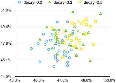
Figure 3: Comparison of our model variations in sentiment classification task when considering consecutive n-grams only (decaying factor $\lambda=0$) and when considering non-consecutive n-grams ($\lambda>0$). Modeling non-consecutive n-gram features leads to better performance.

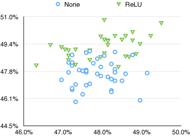
Figure 4: Applying ReLU activation on top of tensor-based feature mapping leads to better performance in sentiment classification task. Runs with no activation are plotted as blue circles.

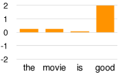
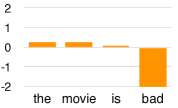
(1) positive prediction	(2) negative prediction		(3) negative prediction	(4) positive prediction
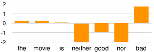
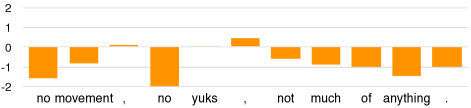
(5) negative prediction		(6) negative prediction (ground truth: negative)
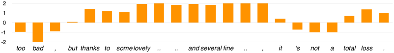
(7) positive prediction (ground truth: positive)

Figure 5: Example sentences and their sentiments predicted by our model trained with root labels. The predicted sentiment scores at each word position are plotted. Examples (1)-(5) are synthetic inputs, (6) and (7) are two real inputs from the test set. Our model successfully identifies negation, double negation and phrases with different sentiment in one sentence.

Number of layers

We plot the fine-grained sentiment classification accuracies obtained during hyperparameter grid search. Figure 2 illustrates how the number of feature layers impacts the model performance. As shown in the figure, adding higher-level features clearly improves the classification accuracy across various hyperparameter settings and initializations.

Non-consecutive n-gram features

We also analyze the effect of modeling non-consecutive n-grams. Figure 3 splits the model accuracies according to the choice of span decaying factor $\lambda$. Note when $\lambda=0$, the model applies feature extractions to consecutive n-grams only. As shown in Figure 3, this setting leads to consistent performance drop. This result confirms the importance of handling non-consecutive n-gram patterns.

Non-linear activation

Finally, we verify the effectiveness of rectified linear unit activation function (ReLU) by comparing it with no activation (or identity activation $f(x)=x$). As shown in Figure 4, our model with ReLU activation generally outperforms its variant without ReLU. The observation is consistent with previous work on convolutional neural networks and other neural network models.

7.3 Example Predictions

Figure 5 gives examples of input sentences and the corresponding predictions of our model in fine-grained sentiment classification. To see how our model captures the sentiment at different local context, we apply the learned softmax activation to the extracted features at each position without taking the average. That is, for each index $i$, we obtain the local sentiment $p=\text{softmax}\left(\mathbf{W}^{\top}\left(z^{(1)}[i]\oplus z^{(2)}[i]\oplus z^{(3)}[i]\right)\right)$. We plot the expected sentiment scores $\sum_{s=-2}^{2}s\cdot p(s)$, where a score of 2 means “very positive”, 0 means “neutral” and -2 means “very negative”. As shown in the figure, our model successfully learns negation and double negation. The model also identifies positive and negative segments appearing in the sentence.

8 Conclusion

We proposed a feature mapping operator for convolutional neural networks by modeling n-gram interactions based on tensor product and evaluating all non-consecutive n-gram vectors. The associated parameters are maintained as a low-rank tensor, which leads to efficient feature extraction via dynamic programming. The model achieves top performance on standard sentiment classification and document categorization tasks.

References

- [Bahdanau et al., 2014] Dzmitry Bahdanau, Kyunghyun Cho, and Yoshua Bengio. 2014. Neural machine translation by jointly learning to align and translate. arXiv preprint arXiv:1409.0473.
- [Bengio et al., 2003] Yoshua Bengio, Réjean Ducharme, Pascal Vincent, and Christian Janvin. 2003. A neural probabilistic language model. The Journal of Machine Learning Research, 3:1137–1155.
- [Bergstra et al., 2010] James Bergstra, Olivier Breuleux, Frédéric Bastien, Pascal Lamblin, Razvan Pascanu, Guillaume Desjardins, Joseph Turian, David Warde-Farley, and Yoshua Bengio. 2010. Theano: a CPU and GPU math expression compiler. In Proceedings of the Python for Scientific Computing Conference (SciPy).
- [Chen and Manning, 2014] Danqi Chen and Christopher D Manning. 2014. A fast and accurate dependency parser using neural networks. In Proceedings of the 2014 Conference on Empirical Methods in Natural Language Processing (EMNLP), pages 740–750.
- [Collobert and Weston, 2008] R. Collobert and J. Weston. 2008. A unified architecture for natural language processing: Deep neural networks with multitask learning. In International Conference on Machine Learning, ICML.
- [Collobert et al., 2011] Ronan Collobert, Jason Weston, Léon Bottou, Michael Karlen, Koray Kavukcuoglu, and Pavel Kuksa. 2011. Natural language processing (almost) from scratch. The Journal of Machine Learning Research, 12:2493–2537.
- [Devlin et al., 2014] Jacob Devlin, Rabih Zbib, Zhongqiang Huang, Thomas Lamar, Richard Schwartz, and John Makhoul. 2014. Fast and robust neural network joint models for statistical machine translation. In 52nd Annual Meeting of the Association for Computational Linguistics.
- [Duchi et al., 2011] John Duchi, Elad Hazan, and Yoram Singer. 2011. Adaptive subgradient methods for online learning and stochastic optimization. The Journal of Machine Learning Research, 12:2121–2159.
- [Gao et al., 2014] Jianfeng Gao, Patrick Pantel, Michael Gamon, Xiaodong He, Li Deng, and Yelong Shen. 2014. Modeling interestingness with deep neural networks. In Proceedings of the 2013 Conference on Empirical Methods in Natural Language Processing.
- [Hinton et al., 2012] Geoffrey E Hinton, Nitish Srivastava, Alex Krizhevsky, Ilya Sutskever, and Ruslan R Salakhutdinov. 2012. Improving neural networks by preventing co-adaptation of feature detectors. arXiv preprint arXiv:1207.0580.
- [Irsoy and Cardie, 2014] Ozan Irsoy and Claire Cardie. 2014. Deep recursive neural networks for compositionality in language. In Advances in Neural Information Processing Systems.
- [Iyyer et al., 2015] Mohit Iyyer, Varun Manjunatha, Jordan Boyd-Graber, and Hal Daume III. 2015. Deep unordered composition rivals syntactic methods for text classification. In Association for Computational Linguistics.
- [Kalchbrenner and Blunsom, 2013] Nal Kalchbrenner and Phil Blunsom. 2013. Recurrent continuous translation models. In Proceedings of the 2013 Conference on Empirical Methods in Natural Language Processing (EMNLP 2013), pages 1700–1709.
- [Kalchbrenner et al., 2014] Nal Kalchbrenner, Edward Grefenstette, and Phil Blunsom. 2014. A convolutional neural network for modelling sentences. In Proceedings of the 52th Annual Meeting of the Association for Computational Linguistics.
- [Kartsaklis et al., 2012] Dimitri Kartsaklis, Mehrnoosh Sadrzadeh, and Stephen Pulman. 2012. A unified sentence space for categorical distributional-compositional semantics: Theory and experiments. In In Proceedings of COLING: Posters.
- [Kim, 2014] Yoon Kim. 2014. Convolutional neural networks for sentence classification. In Proceedings of the Empiricial Methods in Natural Language Processing (EMNLP 2014).
- [Küchler and Goller, 1996] Andreas Küchler and Christoph Goller. 1996. Inductive learning in symbolic domains using structure-driven recurrent neural networks. In KI-96: Advances in Artificial Intelligence, pages 183–197.
- [Le and Mikolov, 2014] Quoc Le and Tomas Mikolov. 2014. Distributed representations of sentences and documents. In Proceedings of the 31st International Conference on Machine Learning (ICML-14), pages 1188–1196.
- [Le and Zuidema, 2015] Phong Le and Willem Zuidema. 2015. Compositional distributional semantics with long short term memory. In Proceedings of Joint Conference on Lexical and Computational Semantics (*SEM).
- [LeCun et al., 1998] Y. LeCun, L. Bottou, Y. Bengio, and P. Haffner. 1998. Gradient-based learning applied to document recognition. Proceedings of the IEEE, 86(11):2278–2324, November.
- [Lei et al., 2014] Tao Lei, Yu Xin, Yuan Zhang, Regina Barzilay, and Tommi Jaakkola. 2014. Low-rank tensors for scoring dependency structures. In Proceedings of the 52th Annual Meeting of the Association for Computational Linguistics. Association for Computational Linguistics.
- [Mikolov et al., 2010] Tomas Mikolov, Martin Karafiát, Lukas Burget, Jan Cernockỳ, and Sanjeev Khudanpur. 2010. Recurrent neural network based language model. In INTERSPEECH 2010, 11th Annual Conference of the International Speech Communication Association, Makuhari, Chiba, Japan, September 26-30, 2010, pages 1045–1048.
- [Mikolov et al., 2013] Tomas Mikolov, Kai Chen, Greg Corrado, and Jeffrey Dean. 2013. Efficient estimation of word representations in vector space. CoRR.
- [Mitchell and Lapata, 2008] Jeff Mitchell and Mirella Lapata. 2008. Vector-based models of semantic composition. In ACL, pages 236–244.
- [Pennington et al., 2014] Jeffrey Pennington, Richard Socher, and Christopher D Manning. 2014. Glove: Global vectors for word representation. volume 12.
- [Pollack, 1990] Jordan B Pollack. 1990. Recursive distributed representations. Artificial Intelligence, 46:77–105.
- [Shen et al., 2014] Yelong Shen, Xiaodong He, Jianfeng Gao, Li Deng, and Grégoire Mesnil. 2014. Learning semantic representations using convolutional neural networks for web search. In Proceedings of the companion publication of the 23rd international conference on World wide web companion, pages 373–374. International World Wide Web Conferences Steering Committee.
- [Socher et al., 2011a] Richard Socher, Cliff C. Lin, Andrew Y. Ng, and Christopher D. Manning. 2011a. Parsing natural scenes and natural language with recursive neural networks. In Proceedings of the 26th International Conference on Machine Learning (ICML).
- [Socher et al., 2011b] Richard Socher, Jeffrey Pennington, Eric H Huang, Andrew Y Ng, and Christopher D Manning. 2011b. Semi-supervised recursive autoencoders for predicting sentiment distributions. In Proceedings of the Conference on Empirical Methods in Natural Language Processing, pages 151–161. Association for Computational Linguistics.
- [Socher et al., 2013] Richard Socher, Alex Perelygin, Jean Wu, Jason Chuang, Christopher D. Manning, Andrew Y. Ng, and Christopher Potts. 2013. Recursive deep models for semantic compositionality over a sentiment treebank. In Proceedings of the 2013 Conference on Empirical Methods in Natural Language Processing, pages 1631–1642, October.
- [Sutskever et al., 2014] Ilya Sutskever, Oriol Vinyals, and Quoc VV Le. 2014. Sequence to sequence learning with neural networks. In Advances in Neural Information Processing Systems, pages 3104–3112.
- [Tai et al., 2015] Kai Sheng Tai, Richard Socher, and Christopher D Manning. 2015. Improved semantic representations from tree-structured long short-term memory networks. In Proceedings of the 53th Annual Meeting of the Association for Computational Linguistics.
- [Turian et al., 2010] Joseph Turian, Lev Ratinov, and Yoshua Bengio. 2010. Word representations: A simple and general method for semi-supervised learning. In Proceedings of the 48th Annual Meeting of the Association for Computational Linguistics, ACL ’10. Association for Computational Linguistics.
- [Yih et al., 2014] Wen-tau Yih, Xiaodong He, and Christopher Meek. 2014. Semantic parsing for single-relation question answering. In Proceedings of ACL.
- [Zhang and LeCun, 2015] Xiang Zhang and Yann LeCun. 2015. Text understanding from scratch. arXiv preprint arXiv:1502.01710.