Student Understanding of the Boltzmann Factor

Abstract

We present results of our investigation into student understanding of the physical significance and utility of the Boltzmann factor in several simple models. We identify various justifications, both correct and incorrect, that students use when answering written questions that require application of the Boltzmann factor. Results from written data as well as teaching interviews suggest that many students can neither recognize situations in which the Boltzmann factor is applicable, nor articulate the physical significance of the Boltzmann factor as an expression for multiplicity, a fundamental quantity of statistical mechanics. The specific student difficulties seen in the written data led us to develop a guided-inquiry tutorial activity, centered around the derivation of the Boltzmann factor, for use in undergraduate statistical mechanics courses. We report on the development process of our tutorial, including data from teaching interviews and classroom observations on student discussions about the Boltzmann factor and its derivation during the tutorial development process. This additional information informed modifications that improved students’ abilities to complete the tutorial during the allowed class time without sacrificing the effectiveness as we have measured it. These data also show an increase in students’ appreciation of the origin and significance of the Boltzmann factor during the student discussions. Our findings provide evidence that working in groups to better understand the physical origins of the canonical probability distribution helps students gain a better understanding of when the Boltzmann factor is applicable and how to use it appropriately in answering relevant questions.

I Introduction

The study of student understanding of advanced topics is becoming increasingly prevalent in physics education research [1, 2, 3, 4, 5, 6, 7, 8, 9, 10, 11, 12, 13, 14, 15, 16, 17, 18]. Investigating upper-division undergraduate students provides a snapshot of the intellectual journey from novice introductory student to expert physicist that may reveal key components of this transition [19]. Moreover, the National Research Council has recently emphasized the need for more study of advanced undergraduate education in many science disciplines [20]. As part of a broader study on student learning in thermal physics, we have investigated student understanding of the Boltzmann factor with the goal of developing instructional strategies to improve that understanding.

Statistical mechanics provides a mechanism for understanding the emergence of macroscopic phenomena from the collective properties of individual microscopic systems; as such, it is a cornerstone of contemporary physics. However, due to its complexity and sophistication, students do not typically encounter statistical mechanics until late in their undergraduate (or even graduate) studies, and comparatively little research has been done to document student difficulties and successes in this field [21, 22, 17, 18, 13, 15]. This work showed that even after instruction students often struggle to distinguish microstates of a system from macrostates and to appropriately relate the two. The fundamental assumption of statistical mechanics states that all accessible microstates of a system (microscopic arrangements of a system’s particles in phase space) are equally probable [23]. Microstates that share common macroscopic properties (system volume, internal energy, etc.) may be grouped into measurable macrostates. The probability of finding the system in a particular macrostate, $\mathcal{M}_{i}$, is determined by the number of microstates corresponding to that macrostate, i.e., the multiplicity, $\omega_{i}$, normalized by the total number of microstates:

$$P(\mathcal{M}_{i})=\frac{\omega_{i}}{\sum\limits_{j}\omega_{j}}.$$ (1)

Much of the intellectual effort of statistical mechanics is spent defining the relevant properties of the microstates and macrostates and determining the multiplicity given the macroscopic properties of the system .

Loverude reports that many students have difficulty distinguishing microstates and macrostates in the context of binary systems [17]. In one question he asked students, after flipping six coins, if the probability of getting five heads was more than, less than, or equal to the probability of getting six heads; about 20% of the students incorrectly stated that the probabilities were the same, often claiming, “all probabilities have equal occurrences,” which is true for microstates but not for macrostates [17, p. 190]. In another question, students had to compare the probabilities of a six-child family having two different sequences of boys and girls (GBGBBG vs. BGBBBB). Over one third of students incorrectly stated that the second sequence was less probable because families are more likely to have equal numbers of boys and girls rather than only one girl out of six, thus connecting the probabilities of a macrostate (the relative number of boys and girls) to an individual microstate (a specific birth sequence).

Loverude also provides evidence that students struggle to distinguish microstates from macrostates, especially in the context of interacting systems. In the context of Einstein’s model for a solid lattice structure, Loverude asked students to determine the most likely energy distribution between two lattices of different sizes [18]. About 40% of students incorrectly stated that the most probable macrostate is the one in which each solid has the same amount of energy and disregarded the number of oscillators within each lattice. Loverude also reports that students often add the multiplicities of interacting Einstein solids to determine the total multiplicity rather than appropriately multiplying them [18].

A key aspect of equilibrium statistical mechanics is that, when dealing with large systems ($\sim 10^{23}$ particles), the most likely state of the system is overwhelmingly the most probable. This result is due to the fact that the statistical spread of the macrostate probability distribution tends to decrease as $\sigma\propto N^{-1/2}$ where $\sigma$ is the standard deviation and $N$ is the number of particles in the system. When $N$ is large, nearly 100% of all microstates exist within a range of macrostates that are virtually indistinguishable from each other; i.e., within the limits of measurable uncertainty. This single most likely “system state” is the equilibrium state (with microscopic fluctuations) of the macroscopic thermodynamic system .

Mountcastle, Bucy, and Thompson studied students’ understanding of probability distributions by asking them to determine the most probable number of “heads” when flipping $N$ coins as well the uncertainty in this value (reported as $a\pm\Delta a$) [22]. About a third of students incorrectly indicated that the relative uncertainty remains constant as $N$ increases, e.g., $\Delta a/a=15\%$ for all cases, and about 20% stated that the uncertainty covers the entire range of possible values (the most probable result is $N/2\pm N/2$). However, students readily recognized that performing additional measurements would reduce the uncertainty of the mean; e.g., using more rain gauges to measure amount of rainfall [22]. Further investigation showed that students have difficulty reconciling the “overwhelmingly probable” equilibrium state with calculations and graphs showing that the probability of the single most likely macrostate actually decreases with increasing $N$: $P_{\textrm{max}}=N!/\left[2^{N}\left(N/2\right)!\left(N/2\right)!\right]$ for the binomial distribution. Some students took this idea to the extreme on the coin toss question by stating that the most probable result of flipping $6\times 10^{23}$ coins is $3\times 10^{23}\pm 1$ heads. The distinction between a single discrete macrostate and an equilibrium thermodynamic “state” (consisting of a range of virtually indistinguishable macrostates) is subtle and requires careful attention by both students and instructors. These results, along with Loverude’s [18], provide the foundation for studies into students’ understanding of the statistical treatment of thermodynamic systems where states are defined by continuous (rather than discrete) quantities.

The canonical probability distribution defined by the Boltzmann factor has been described as “the quintessential expression of the statistical mechanical approach” [26, p. 109] and “the most powerful tool in all of statistical mechanics” [23, p. 220]. By knowing the possible microscopic energy eigenstates, one may deduce the thermodynamic equilibrium properties of any system at constant temperature, including average internal energy, free energy, entropy, pressure, heat capacity, etc. This connection between microscopic and macroscopic properties is known to be difficult in multiple contexts in physics [27, 28, 29, 30, 17, 18] as well as chemistry [31]. As the core of statistical mechanics is this micro-macro connection, this topic is an optimal context for an investigation of this nature. Our investigation of student understanding of the Boltzmann factor provides additional information about difficulties students have with this connection; these results have implications for studies of more complex systems and topics.

In this paper we present results of our investigation into student understanding of the physical significance and utility of the Boltzmann factor in several simple models. We identify various justifications, both correct and incorrect, that students use when answering written questions that require application of the Boltzmann factor. Results from written data as well as teaching interviews suggest that many students can neither recognize situations in which the Boltzmann factor is applicable, nor articulate the physical significance of the Boltzmann factor as an expression for multiplicity, a fundamental quantity of statistical mechanics. The specific student difficulties seen in the written data led us to develop a guided-inquiry tutorial activity, centered around the derivation of the Boltzmann factor, for use in an undergraduate statistical mechanics course. We report on the development process of our tutorial, including data from teaching interviews and classroom observations on student discussions about the Boltzmann factor and its derivation during the tutorial development process. This additional information informed modifications that improved students’ abilities to complete the tutorial during the allowed class time without sacrificing the effectiveness as we have measured it. Our findings provide evidence that working in groups to better understand the physical origins of the canonical probability distribution helps students gain a better understanding of when the Boltzmann factor is applicable and how to use it appropriately in answering relevant questions.

II The Physics of the Boltzmann Factor

Before discussing our research on student understanding of the Boltzmann factor, it is useful to provide an overview of the physics (and mathematics) of the Boltzmann factor and the canonical partition function. The particular derivation of the Boltzmann factor and the canonical partition function through which students are guided in the tutorial is included in the Appendix.

The underlying assumption of the canonical ensemble is that the thermodynamic system has a fixed equilibrium temperature, a fixed number of particles, and may exchange energy with its surroundings. A standard model for the canonical ensemble is a very small system in equilibrium with a large thermal energy reservoir (free to exchange energy but not particles, see Fig. 1). The Boltzmann factor is a mathematical expression for the probability that a system in equilibrium at a fixed temperature is in a particular energy state,

$$P(\psi_{j})\propto e^{-E_{j}/kT},$$ (2)

where $\psi_{j}$ denotes the microstate with a particular energy $E_{j}$, $k$ is Boltzmann’s constant, and $T$ is the temperature of the system . The decaying exponential form of the Boltzmann factor results from an expression of the multiplicity of the reservoir derived from Boltzmann’s equation,

$$S=k\ln(\omega).$$ (3)

As the energy of the system decreases, the energy (and multiplicity) of the reservoir increases in such a way that the total probability increases (see the Appendix for full details).

The canonical partition function ($Z$) is the result of the normalization constraint that the sum of probabilities [$P(\psi_{j})$] over all $j$ must be unity:

$$\sum\limits_{j}P(\psi_{j}) =\sum\limits_{j}\frac{e^{-E_{j}/kT}}{Z}=1$$ (4)

$$Z =\sum\limits_{i}e^{-E_{i}/kT},$$ (5)

where $Z$ depends on temperature, but is independent of the energy value $E_{j}$ . One may also express the partition function in terms of the energy of a macrostate, $E$:

$$Z =\int\limits_{All~{}E}D(E)\,e^{-E/kT}\,\mathrm{d}E,$$ (6)

where the density of states function, $D(E)$, accounts for the degeneracy (or multiplicity) of the macrostate. In this way the canonical partition function is equally valid for systems with discrete energy microstates, as in Eq. (5), and those with continuous energy distributions, as in Eq. (6).

The canonical partition function can be used to express equilibrium (macroscopic) thermodynamic quantities. For example, the Helmholtz free energy of a system may be written as a function of $Z$,

$$F=-kT\ln(Z);$$ (7)

derivatives of $F$ yield information about the system’s entropy, pressure, magnetization, and many other thermodynamic variables. Moreover, the average energy of a system, $\langle{E}\rangle$, may be expressed as a derivative of the natural logarithm of $Z$. Due to these connections, Schroeder refers to the canonical probability distribution as “the most useful formula in all of statistical mechanics” [23, p. 223]. The canonical partition function and the Boltzmann factor are cornerstones of statistical mechanics, and a thorough understanding of when and how they are useful (when examining an equilibrium system at constant temperature) is essential for study in the field.

Figure 1: Sample system for the Boltzmann factor instructional sequence. An isolated container of an ideal gas is separated into a small system ($C\,$) and a large reservoir ($R\,$). The label “$C\,$” is used to avoid confusion with entropy.

III Student Understanding of the Origin and Utility of the Boltzmann Factor

We gathered data in several different forms to study student understanding of the Boltzmann factor from multiple perspectives. In one investigation, we gave students an ungraded written survey to determine whether or not they use the Boltzmann factor in an appropriate context. Additionally, we conducted teaching experiments with several students as well as classroom observations to assess their understanding of the physical origin and significance of the mathematical expression of the Boltzmann factor. Our results indicate that students often do not use the Boltzmann factor in appropriate contexts, instead using vague notions of lower energies having higher probabilities to make conclusions about the ratios of these probabilities. Moreover, we find that students may not recognize the physical significance of the Boltzmann factor, even after having memorized its mathematical derivation.

Figure 2: Probability Ratios Question (PRQ): given as an ungraded survey before tutorial instruction.

III.1 Student use of the Boltzmann factor in appropriate contexts

One desired result of teaching students about the Boltzmann factor is that they will recognize applicable situations and use it appropriately to make claims about probabilities of the occupation of specific energy states. The probability ratios question (PRQ, shown in Fig. 2) probes their ability to do this. The correct solution to the PRQ requires students to recognize three pieces of information:

• The probability of a single particle being in each of three energy states is proportional to the Boltzmann factor for each state

• A ratio of exponential functions is the exponential of the difference of their exponents

• The differences in energies between adjacent states are the same for each particle ($\Delta E_{n,n-1}\nobreak=\nobreak 0.05\,\mathrm{eV}$)

The first two items indicate that each ratio of probabilities is an exponential function of the energy difference between the two states. The third item reveals that both pairs of ratios in the PRQ are equal . Students were also considered to have given a correct explanation to part B of the PRQ if they stated that the two ratios were equal because the only difference between the two particles is the energy of the ground state.

III.1.1 Recognizing the need for the Boltzmann factor

The PRQ was administered to students in an upper-division statistical mechanics course at a land-grant research university in the northeastern United States (School 1); data were collected from seven successive classes ($N=50$). Students at School 1 are typically senior undergraduates who have competed studies in classical mechanics, electrodynamics, and quantum mechanics. The PRQ was also administered once in a single-semester upper-division thermal physics course at a comprehensive public university in the western United States (School 2, $N=32$). Students at School 2 are typically junior undergraduates who have completed studies in modern physics and classical mechanics. The PRQ was administered at both schools immediately before students participated in guided-inquiry activities regarding the Boltzmann factor and the canonical partition function (our Boltzmann Factor tutorial, see Sec. IV). At School 1 the activities were used after lecture instruction, and the PRQ was given after lectures. At School 2 the activities were used in place of lecture instruction, and the PRQ was given before instruction to establish a baseline for students’ understanding before the tutorial.

Student responses to the PRQ were coded in two ways: first by the response given (equal to, greater than, less than, or other), second by whether or not the Boltzmann factor was used. Figure 3a shows the response frequencies for the entire seven-year data corpus from School 1, and Fig. 3b shows the response frequencies from School 2. Green diagonal stripes indicate the students who used the Boltzmann factor or stated that the energy of the ground state was irrelevant (in part B) to obtain their chosen answers; these students are considered to have used correct explanations regardless of which answer they chose. .

We used a grounded theory approach to analyze students’ explanations for their responses; the entire data corpus was examined for common trends, yielding categories defined by the data, and all data were reexamined to group them into those defined categories [36, 37]. One goal of our analysis was to focus on describing rather than interpreting students’ explanations while defining the categories. In this way our analysis stays as true to the data as possible by limiting researcher biases and interpretations. This is consistent with Heron’s identification of specific difficulties [38].

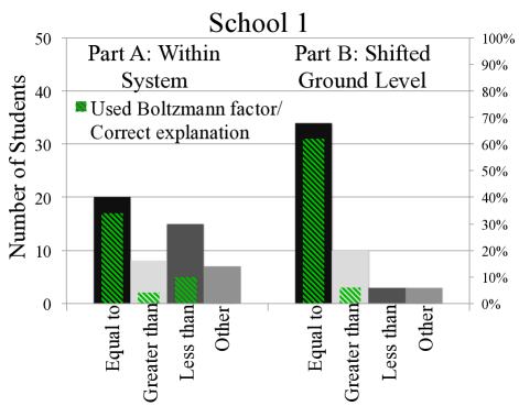
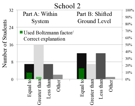
(a)                                                                             (b)

Figure 3: PRQ pretutorial results. a) School 1: after lecture instruction on the Boltzmann factor over seven years ($N\nobreak=\nobreak 50$), b) School 2: before any instruction on the Boltzmann factor in one year ($N\nobreak=\nobreak 32$). The green diagonal stripes indicate the students who used the Boltzmann factor or stated that the energy of the ground state was irrelevant (in part B) to obtain their chosen answers. Students in the “Other” column often provided no explicit answer or stated that there was not enough information to determine the answer. Only 24 students from School 1 and four students from School 2 used the Boltzmann factor on both parts.

The data represented in Fig. 3 suggest two questions: 1) What is the prevalence of invocation of the Boltzmann factor, regardless of the correctness of the response? and 2) How do students justify their answers if they do not apply the Boltzmann factor? To answer the first of these questions, the data show four categories of responses:

• Correct response (equal to) using the Boltzmann factor (or stating that the energy of the ground state was irrelevant in part B)

• Correct response without using the Boltzmann factor

• Incorrect response using the Boltzmann factor

• Incorrect response without using the Boltzmann factor

This coding scheme enables highlighting of the number of students who are and are not invoking the Boltzmann factor to answer the PRQ. A natural question associated with this coding scheme is, how might someone invoke the Boltzmann factor but arrive at an incorrect response? One route is to make a computational error. On the other hand, one could compare the wrong ratios, but do so correctly using the Boltzmann factor. Data also indicate that some students imposed degeneracy terms when using the Boltzmann factor to answer the PRQ. In coding responses, a student who wrote that probability is related to a decaying exponential of the energy was coded as using the Boltzmann factor independent of the final answer obtained. Using the Boltzmann factor and stating that the energy of the ground state is irrelevant were grouped together because both are correct physical justifications for concluding that the ratios of probabilities in part B of the PRQ are equal.

Table 1: Results from the PRQ pretest at both School 1 ($N=50$) and School 2 ($N=32$). Students are grouped by whether or not they gave the correct answer (Equal to) and whether or not they used the Boltzmann factor (or stated that the energy of the ground state was irrelevant in part B).

			Part A			Part B
		Correct	Incorrect	Total	Correct	Incorrect	Total
	Used Bf	34%	14%	48%	62%	6%	68%
S1	No Bf	6%	46%	52%	6%	26%	32%
	Used Bf	9%	3%	12%	16%	0%	16%
S2	No Bf	13%	75%	88%	22%	63%	84%

Table 1 shows the percentages of students who occupy each of the four response categories at each school for both parts of the PRQ. From the data shown in Fig. 3 and Table 1 it is clear that the distribution of responses is different at the two schools. A Fisher’s exact test showed this to be true ($p=0.008$ for part A, $p<0.001$ for part B) [39, 40, 41]. Another Fisher’s exact test showed that students at School 1 are using the Boltzmann factor on the PRQ pretest more than students at School 2 ($p<0.001$ on both parts) . This is not surprising given that students at School 1 had received lecture instruction on the Boltzmann factor, while students at School 2 had not. On the other hand, only 48% of students at School 1 used the Boltzmann factor on part A and only 68% did so on part B, indicating that lecture instruction alone was not sufficient for all students to gain a robust understanding of when and how to use the Boltzmann factor.

The most common incorrect response at School 1 for both parts of the PRQ is that $P(0.10\mathrm{~{}eV})/P(0.05\mathrm{~{}eV})\nobreak<\nobreak{P(0.05\mathrm{~{}eV})}/P(0.00\mathrm{~{}eV})$ (“less than” for part A and “greater than” for part B; see Table 2). These answers are considered consistent because the second and third energy levels in particle B have the same numerical values as the first and second energy levels in particle A, respectively. A Fisher’s exact test shows the distribution of “less than” and “greater than” responses from School 1 to be significantly different for part A as compared to part B ($p\nobreak=\nobreak 0.035$). However, the data from School 2 show the exact opposite trend: more students answer “greater than” for part A and “less than” for part B (see Fig. 3b and Table 2). A Fisher’s exact test shows that this difference at School 2 approaches significance ($p=0.061$). Additional tests show that the results from School 2 are significantly different from those at School 1 ($p=0.038$ for part A and $p=0.036$ for part B).

Table 2: Pretest Response Comparison: “greater than” vs. “less than.” Numbers shown indicate the percentage of incorrect responses at each of the two schools. This is necessary because significantly more students answered the PRQ correctly at School 1 than at School 2. Only by looking at the percentages of incorrect responses can meaningful comparisons be made.

	Part A		Part B
	greater than	less than	greater than	less than
School 1	23%	38%	44%	19%
School 2	54%	25%	26%	44%

Figure 3a also shows that students at School 1 are more likely to answer part B correctly (which discusses an effective shift in the ground state energy of a system) than part A (comparing two different sets of probabilities for states within the same system), with only 34% using the Boltzmann factor to obtain the correct response on part A compared to 64% providing a correct explanation on part B (statistically significant, $p=0.035$). One student at School 1 justified his response for part B in stating that, “…it does not matter what the ‘baseline’ is, just the amount of energy added.” This higher performance on part B could be a result of our coding scheme in that explanations involving comments about the arbitrariness of the ground state energy were considered correct for part B regardless of the student’s response to part A. This phenomenon is not significantly observed at School 2 (see Fig. 3b, Fisher’s exact test yields $p=0.45$).

III.1.2 Incorrect reasoning about probability ratios

The justifications students used to support their final answers were sorted into several categories developed using a grounded theory approach. At School 1, 24 students (out of 50) used the Boltzmann factor within their explanation of their answers on the PRQ; only four out of 32 students at School 2 used the Boltzmann factor. Of the remaining students at each school, roughly half (15 out of 26 at School 1 and 13 out of 28 at School 2) used a ranking of probabilities as their primary justification; e.g., $P_{A}(1)>P_{A}(2)>P_{A}(3)$. An additional five students at School 2 stated that the lowest energy is most probable but did not make claims about the relative probabilities of energy states 2 and 3. Using probability ranking, either explicit or implied, is the most common incorrect justification at both schools, and no students provided a physical explanation for why the probabilities of the various energy levels would be ranked as they claimed.

Of the students who ranked the probabilities to justify their answers, eight students at School 1 and seven at School 2 made claims about the relative difference in probability between states 1 and 2 and between states 2 and 3. Some claims were made in sentence form, e.g., “… it is more likely that the system will have less energy so the difference between [states] 3 & 2 is less than [between states] 2 and 1” (student’s emphasis); other claims took the form of a mathematical expression, e.g., “$P_{A}(1)-P_{A}(2)\nobreak>P_{A}(2)-P_{A}(3)$.” Both of these statements imply the idea that $P_{A}(1)\gg P_{A}(2)>P_{A}(3)$. All seven students at School 2 used this idea to claim that $P_{A}(3)/P_{A}(2)>P_{A}(2)/P_{A}(1)$. However, the students at School 1 used similar reasoning to come to three different conclusions:

$$P_{A}(1)\gg P_{A}(2)>P_{A}(3) \rightarrow\frac{P_{A}(3)}{P_{A}(2)}>\frac{P_{A}(2)}{P_{A}(1)};$$ (8)

$$P_{A}(1)>P_{A}(2)\gg P_{A}(3) \rightarrow\frac{P_{A}(3)}{P_{A}(2)}<\frac{P_{A}(2)}{P_{A}(1)};$$ (9)

$$P_{A}(1)\gg P_{A}(2)\gg P_{A}(3) \rightarrow\frac{P_{A}(3)}{P_{A}(2)}=\frac{P_{A}(2)}{P_{A}(1)}.$$ (10)

Interestingly, this third case was used to justify a correct response.

In each of these cases, students seem to be considering the probabilities in pairs and using the relative difference between each pair to compare the ratios of the pairs. This is consistent with a strategy for comparing fractions that Smith refers to as Compare Numerator-Denominator Differences (NDD) [43]. The NDD strategy is categorized by students using the within-fraction difference between the denominator and the numerator as a comparative measure. Examples of the NDD strategy in Smith’s study include students determining that $3/5=5/7$ (because $5-3=7-5=2$) and that $14/24>7/12$ (because $24-14>12-7$) [43]. In our case, students are explicitly or implicitly using the differences between the probabilities as justification for comparing their ratios. Arons cites difficulties interpreting ratios as one of the most prevalent cognitive gaps for students at the secondary and undergraduate levels [44, p. 4–9].

Students who ranked the probabilities as simply $P_{A}(1)>P_{A}(2)>P_{A}(3)$ also made claims that are consistent with some of Smith’s other classifications. Using this ranking to claim that $P_{A}(3)/P_{A}(2)>P_{A}(2)/P_{A}(1)$ (“greater than” on part A) is consistent with Smith’s Denominator Principle (DP, fractions with larger denominators are smaller than fractions with smaller denominators), and using this ranking to claim that $P_{A}(3)/P_{A}(2)<P_{A}(2)/P_{A}(1)$ (“less than” on part A) is consistent with both the Numerator Principle (NP, fractions with larger numerators are larger) and Larger Components (LC, fractions with larger numerators and denominators are larger) [43]. However, since no student admitted to exclusively using either the numerator or the denominator of each ratio to compare the two, we cannot be certain that students used these strategies, only that the students’ final responses are consistent with their use.

Students who used probability rankings to justify their answers were categorized as being consistent with one (or more) of Smith’s strategies. Reliability of the categories for our classification was checked by an independent classification of the data from School 2. There was initial agreement for 72% of the student responses; after discussion and negotiation, agreement of 91% and at least partial agreement of 97% of students was obtained (one analysis placed some students simultaneously in two categories, while the other only agreed on one of the categories for this group).

At both School 1 and School 2 more student responses were aligned with the NDD strategy than either DP or NP/LC, and no significant differences were found between the two student populations in terms of their use of these strategies. In many cases it is unclear precisely why a student chose the response s/he did based on the ranking provided, but it is interesting to note the similarities between their claims and those made by the adolescent students in Smith’s study.

The key difficulty identified so far is that many students do not apply the Boltzmann factor when it is appropriate to do so, even after lecture instruction. Instead, these students provide responses that are consistent with using novice-like reasoning strategies for comparing ratios. Most students recognized that lower energies are more probable, but they offered no physical justification for why this is so and couldn’t use this information alone to make conclusions about the probability ratios in question.

III.2 Recitation of a mathematical derivation without physical understanding

In an effort to probe student understanding of the Boltzmann factor more deeply, we conducted individual interviews with four students at School 1 after classroom instruction in the first year of tutorial implementation to determine their familiarity with the Boltzmann factor, its applications, and its origin. Two interview participants had participated in the first half of the Boltzmann Factor tutorial during class (in which they discussed the definitions of macrostates, microstates, and multiplicity for the microcanonical and canonical ensembles, see Sec. IV), while the other two had not seen the tutorial. The interviews were conducted in the style of a teaching experiment [45, 46, 15] and consisted of asking students to complete a guided-inquiry activity that started with asking them to consider how probability relates to multiplicity in the divided container ($C$-$R\,$) scenario (see Fig. 1) and culminated with the derivation of the Boltzmann factor .

The teaching experiment is a unique form of interview as “it is an acceptable outcome…for students to modify their thinking” during the course of the interview [46]. According to Steffe and Thompson, “a teaching experiment involves a sequence of teaching episodes…[including] a teaching agent, one or more students, a witness of the teaching episodes, and a method of recording what transpires during the episode” [45]. For our purposes the interviewer alternated roles as both teaching agent and witness during each interview. In a sense, the activities used during the interview may also be seen as a teaching agent as they included tasks for students to complete, and students interacted with the document in an intellectual manner. Our goal for the interviews was not to simply determine students’ understanding of the Boltzmann factor, but rather to examine how well they could complete instructional tasks based on previous knowledge related to the Boltzmann factor. Students worked on their own; the interviewer solicited explanations for their work and gave assistance when required. Field notes were taken during the interviews, and students’ written work was collected afterward.

Table 3: Sample energy & multiplicity values for the “toy model” system ($C$) and reservoir ($R$; see Fig. 1). This table was presented to students during the teaching interviews and is also used in the Boltzmann Factor tutorial. A key element of this situation is that the combined energy of $C$ and $R$ is a fixed value, $E_{tot}$.

$E_{C}$	$\omega_{C}$	$E_{R}$	$\omega_{R}$
$E_{1}$	1	$E_{tot}-E_{1}$	$3\times 10^{18}$
$E_{2}$	1	$E_{tot}-E_{2}$	$5\times 10^{19}$
$E_{3}$	1	$E_{tot}-E_{3}$	$4\times 10^{17}$
$E_{4}$	1	$E_{tot}-E_{4}$	$1\times 10^{20}$
$E_{5}$	1	$E_{tot}-E_{5}$	$7\times 10^{18}$

Results from the teaching interviews provide further evidence of the need for the Boltzmann Factor tutorial, especially with regard to the origin of the Boltzmann factor itself. None of the interview participants found the tasks to be trivial, and none correctly articulated how the Boltzmann factor as an expression of probability relates to multiplicity prior to the interview. A major finding during these interviews was the identification of students’ difficulties in executing the Taylor series expansion as part of the derivation of the Boltzmann factor; we reported these difficulties previously [15].

One episode during one of the student interviews was of particular interest. One student (Joel , who had participated in portions of the Boltzmann Factor tutorial in class) was very familiar with the applications of the Boltzmann factor and seemed to be just as familiar with its origin. In one portion of the activity, students were given a table of multiplicities for various discrete system energy levels and asked to determine the most probable macrostate (see Table 3). The desired result was for students to conclude that the macrostate with the greatest reservoir multiplicity would be the most probable. Joel wanted to use the Boltzmann factor rather than thinking about multiplicities, even though no information had been given about the relative energy values . The interviewer asked Joel to show where the Boltzmann factor came from before applying it to this situation, at which point Joel quoted the textbook derivation of the Boltzmann factor practically verbatim. The final portion of Baierlein’s mathematical derivation is as follows [26, p. 92],

$$P(\psi_{j}) =\textrm{const}\times\left(\parbox{126.47249pt}{multiplicity of reservoir when it has energy $E_{tot}-E_{j}$}\right)$$ (11)

$$P(\psi_{j}) =\textrm{const}\times\exp\left[\frac{1}{k}S_{R}(E_{tot}-E_{j})\right]$$ (12)

$$P(\psi_{j}) =\textrm{const}\times\exp\frac{1}{k}\left[S_{R}(E_{tot})\!+\!\frac{\partial S_{R}}{\partial E_{R}}\textrm{\hskip 1.42262pt\rule[-8.53581pt]{0.7113pt}{22.76219pt}}_{{}_{\hskip 0.7113ptE_{{}_{tot}}}}\textrm{}\!\!\!\!\left(-E_{j}\right)\right]$$ (13)

$$P(\psi_{j}) =\textrm{(new constant)}\times\exp\left(-E_{j}/kT\right).$$ (14)

This derivation exploits the fact that the combined energy of the system and reservoir ($E_{tot}$) is a fixed quantity in order to write the energy of the reservoir ($E_{R}$) in terms of the energy of the system ($E_{j}$).

Joel’s ability to reproduce the derivation might suggest an understanding of the physical significance of the Boltzmann factor. However, when asked how the multiplicity of the reservoir relates to the Boltzmann factor, Joel was at a loss. During his replication of the derivation of the Boltzmann factor he had implicitly written that it was proportional to $\omega_{R}$ (connecting Eqs. 11 and 14), but without explicit help from the interviewer, Joel could not recognize that the multiplicity of the reservoir when it has energy, $E_{tot}-E_{j}$ (RHS of Eq. (11)), is proportional to the exponential function, $\exp\left(-E_{j}/kT\right)$ (RHS of Eq. (14)). Furthermore, Joel had great difficulty relating the physical example used in the textbook (a “bit of cerium magnesium nitrate…in good thermal contact with a relatively large copper disc” [26, p. 91]) to the ideal gas example used during our interview. He was unable to recognize and articulate the important physical characteristics of each scenario that make the Boltzmann factor applicable; e.g., a system with fixed temperature and variable energy. Joel’s failure to make these connections suggests an incomplete understanding of the physical reasoning used to derive the Boltzmann factor, even after memorizing the textbook derivation.

Results from the teaching interviews and the PRQ suggest that many students can neither recognize situations in which the Boltzmann factor is applicable, nor articulate the physical significance of the Boltzmann factor as an expression for multiplicity, one of the fundamental quantities of statistical mechanics. These difficulties prompted our development of the Boltzmann Factor tutorial to help students better understand the physical origin of the Boltzmann factor and how it may be applied in various contexts.

IV Design and Implementation of the Boltzmann Factor tutorial

Given students’ apparent lack of recognition of when to apply the Boltzmann factor to a physical scenario, we designed a guided-inquiry tutorial activity to lead students through its derivation and encourage deep cognitive connections between the physical quantities involved. The derivation chosen for use in the Boltzmann Factor tutorial is included in the Appendix and may be found in many widely used textbooks, including the one used at the primary research site [26].

Our Boltzmann Factor tutorial gives students the opportunity to productively struggle with the connections between the mathematical formalism and the physical interpretations within the derivation of the Boltzmann factor [15]. Fostering physics-mathematics connections, such as gaining facility with taking limits and making approximations, as well as knowing when to take these steps, is an important and nontrivial component of upper-division courses as students transition from novices to experts in the field [19].

The desired student outcomes during the tutorial are consistent with the concept of productive disciplinary engagement (PDE) [51]. The small group setting, with explicit instructions to discuss responses and reasoning with group mates, fosters engagement, which is evident through student-student discourse. Because disciplinary content is the core of the tutorial, most engagement in a tutorial constitutes disciplinary engagement. Finally, Engle and Conant define productive disciplinary engagement as episodes where student are making progress in their engagement with the content [51]. Evidence of this productivity includes students recognizing their confusion about a concept or making a new connection as a result of the interaction. Indeed, the tutorial pedagogy and the materials themselves provide a setting designed to foster PDE. The pedagogy used in the canonical set of tutorials, Tutorials in Introductory Physics, to address specific student difficulties, fully matches the parameters of PDE [52][53, p. iii]. Our primary goal is that students discuss topics in a way that helps them progress through the tutorial tasks while gaining a better understanding of those topics (discussing relevant concepts, synthesizing information, engaging with the connections between the mathematics and the physics, etc.). While in some cases other, less time-consuming pedagogical approaches may also foster PDE and help students with specific difficulties, in this case the depth of the content and the difficulty of the sequence of steps in the derivation of the Boltzmann factor suggested that a tutorial would be the most effective way to achieve this. Given that a lecture on this topic typically uses an entire class period, we expected the tutorial would occupy a full class period as well as some time outside of class.

IV.1 The Boltzmann Factor Tutorial

The Boltzmann Factor tutorial begins by asking students to consider an isolated container of an ideal gas. They are guided to recognize that the container has a fixed internal energy ($E_{tot}$) and that all accessible microstates are equally probable.

Once the properties of the contents of the isolated container have been established, the students are presented with a scenario in which the container of ideal gas is separated into relatively small and large sections (see Fig. 1). The small system of interest ($C\,$) is said to be in thermal equilibrium with the large reservoir ($R\,$), and the students are asked to compare the values of various thermodynamic properties of $C$ to those of $R$ to highlight the fact that the intensive properties (temperature, pressure) will have the same value for both $C$ and $R$, while the values of the extensive properties (volume, number of particles, internal energy) of $C$ are much smaller than those of $R$.

The third section of the tutorial uses the fact that the multiplicities of $C$ and $R$ are so different ($\omega_{C}\nobreak\ll\nobreak\omega_{R}$) to justify a single-particle “toy model” in which $\omega_{C}\nobreak=\nobreak 1$ ($\omega_{tot}\nobreak=\nobreak\omega_{C}\,\omega_{R}\nobreak=\nobreak\omega_{R}$), and the energy of $C$ can only take on a handful of discrete values, $E_{C}\nobreak\in\nobreak\{E_{j}\}\nobreak=\nobreak\{E_{1},E_{2},\dots\}$ (see Table 3). The students are asked to determine which system microstate ($j=1$, 2, 3, 4, or 5) is most probable and which is least probable. The desired solution is that the system microstate in which the macrostate of $R$ has the largest multiplicity ($\omega_{R}$) is the most probable ($E_{4}$ in Table 3) because all reservoir microstates are equally likely. Careful consideration of the relative probabilities of each macrostate leads to the proportionality between the probability of the $j^{\mathrm{th}}$ microstate of $C$ and the multiplicity of the reservoir: $P(\psi_{j})\nobreak\propto\nobreak\omega_{R}(\psi_{j})$.

The final section of the Boltzmann Factor tutorial is the derivation of the Boltzmann factor itself. The core of this derivation is a Taylor series expansion of $S_{R}(E_{R})$ about the value $E_{R}\nobreak=E_{tot}$ to obtain the expression for $S_{R}$ as a linear function of $E_{C}$ given in Eq. (20) [15]. The students are explicitly asked to consider the physical significance of each term in the expansion and to determine the final linear expression on their own. Then, using the relationship between entropy and multiplicity in Eq. (3), they are guided to derive an expression for $\omega_{R}$:

$$\omega_{R}=e^{S_{R}/k}=e^{S_{R}(E_{tot})/k-E_{C}/kT},$$ (15)

and because $S_{R}(E_{tot})$ is a constant,

$$\omega_{R}\propto e^{-E_{C}/kT},$$ (16)

i.e., the Boltzmann factor. Students find that $P(\psi_{j})\nobreak\propto\nobreak\omega_{R}(\psi_{j})$ and that $\omega_{R}(\psi_{j})\nobreak\propto e^{-E_{j}/kT}$, leading to the proportionality in Eq. (2). Finally, they obtain the expression for the canonical partition function, $Z$, by normalizing the probability.

The post-tutorial homework assignment is an application of the Boltzmann factor to a three-state system with unevenly spaced energy levels. Students are asked various questions about the ratios of probabilities of the system being in a particular state. These questions are similar to the PRQ but the students are given specific values for $T$ and $N$ and asked to determine numerical values for the probability ratio rather than compare two different ratios. They are also asked to determine an expression for the generic ratio between the probabilities of any two energy levels. This homework assignment was used as a continuation of the tutorial, not as an assessment or research tool.

IV.2 Tutorial Implementation

At School 1, the Boltzmann Factor tutorial was implemented after all lecture instruction on the Boltzmann factor. Students were given one 50-minute class period to complete the tutorial. The course instructor and one additional facilitator were available during the tutorial session as observers and facilitators . No course credit is offered for participation in the tutorial itself, but the course grade does include a component for class participation. Several groups were videotaped during tutorial sessions (in three years of classes) to monitor tutorial progress and document student reasoning regarding the Boltzmann factor and related topics.

The Boltzmann Factor tutorial was implemented at School 2 once in place of lecture instruction. Students were given one 50-minute class period and an additional 20 minutes during the next period to complete the tutorial. As described in Sec. III.1, the PRQ was administered as a pretest at both institutions before tutorial instruction, and a similar question was used on course examinations.

V Findings during implementation of the Boltzmann factor tutorial

An interesting question is whether recognizing when to use the Boltzmann factor serves as a direct proxy for an understanding of the physical significance and meaning of the expression — its origin and why it describes the relative occupation of states. Instructors typically assume that this is the outcome of presenting the derivation of such functions to students: that the clear description of the steps of the derivation, including the explicit connections between the mathematical steps and the physical constraints, assumptions, etc. that drive the mathematics, provides students with the intended insight. Thus the subsequent assumption is that the proper invocation of the Boltzmann factor implies an understanding of its meaning and significance. However, in the process of pilot-testing the Boltzmann Factor tutorial we observed that this is not necessarily the case. We have evidence from students working through sections of the tutorial either in class or during teaching interviews that suggest that (a) the students do not have a sense of the physical basis for the Boltzmann factor before the tutorial and (b) the sequencing of the tutorial provides the students the opportunity to gain an understanding and appreciation for this physical foundation.

Below we describe the findings from the data collected during and after tutorial implementation. These data — collected in written and video form — provide evidence to support the claim that the activities the students work through in the tutorial improve both students’ ability to apply the Boltzmann factor appropriately and their understanding of the physical basis for the Boltzmann factor, including the connections between some of the mathematical steps and the physical scenario.

Figure 4: PRQ Analog: developed by instructor at School 2. Administered on a course exam once at School 1 and at School 2.

V.1 Improving student use of the Boltzmann factor in appropriate contexts

In order to probe the effect of tutorial instruction on student tendency to invoke the Boltzmann factor in an appropriate situation, we administered written post-tests at both schools on midterm examinations. The PRQ was given on a course examination after the Boltzmann Factor tutorial in two years at School 1. A similar question, referred to as the PRQ Analog (shown in Fig. 4), was developed by the instructor at School 2 and asked on a course exam in one year at both institutions. The PRQ Analog requires students to apply the same knowledge as is used to correctly answer the PRQ: that the probability of a particle being in one of the energy states is proportional to the Boltzmann factor, and that a ratio of probabilities would be equivalent to a ratio of Boltzmann factors, which depends only on the difference between the energy levels. However, the PRQ Analog adds some complexity by using systems with energy levels that are not evenly spaced and requiring students to recognize that the number of particles occupying each energy level will be proportional to the probability of a single particle having that energy. Despite this added complexity, Fig. 5 shows that students’ use of the Boltzmann factor was very similar on both the PRQ and PRQ Analog exam questions.

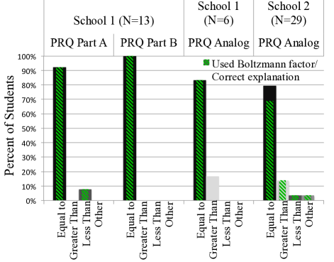
Figure 5: Post-tutorial results from PRQ and PRQ Analog, administered during course examinations. The green diagonal stripes indicate the students who used the Boltzmann factor or stated that the energy of the ground state was irrelevant (in part B) to obtain their chosen answer(s). For the PRQ Analog, “Equal to” corresponds to choice II, “Greater than” to choice I, “Less than” to choice III, and “Other” to choice IV. Data are shown for students who completed the PRQ pretest, participated in the Boltzmann Factor tutorial, and completed either the PRQ or PRQ Analog exam question.

From the three implementations at School 1 there are 19 sets of matched (pre-/post-tutorial) data of students who participated in the Boltzmann Factor tutorial. There are 29 sets of matched data from School 2. Figure 5 shows the exam data from all students broken down by question and school. These data provide evidence that the Boltzmann Factor tutorial helps students recognize the utility of the Boltzmann factor and how to apply it properly in the context of these questions.

The most striking feature of Fig. 5 is that all 13 students at School 1 used appropriate Boltzmann factor reasoning on both parts of the PRQ . Moreover, all but one student at School 1 (about 83%) used the Boltzmann factor correctly to answer the PRQ Analog after tutorial instruction. This is a marked improvement over lecture instruction alone (only about half consistently used the Boltzmann factor on the PRQ pretest). Similarly, all but two students at School 2 (also almost 95%) used the Boltzmann factor to answer the PRQ Analog exam question.

In order to perform statistical analyses to compare the exam results with the pretest results, data were grouped into the four categories discussed in section III.1.1. This reduced coding scheme is necessary because we essentially asked three questions at various times (PRQ parts A and B, and the PRQ Analog): the specific responses to the various questions, e.g., “greater than,” cannot necessarily be considered the same response. As such, the only categories available for grouping responses are either the correct response or one of the incorrect responses; along with this we have the dimension of whether or not a student used the Boltzmann factor appropriately to justify his or her response, consistent with the four categories above. These general categories do not allow claims to be made about how reasoning patterns differ within the incorrect responses, but they do allow comparisons of the frequency with which students use the correct Boltzmann factor reasoning and whether or not it yielded a correct response. Using these categories, a Fisher’s exact test showed that all exam data are statistically similar ($p=0.125$). Additionally, a Fisher’s exact test comparing the data at School 1 showed that the results from the exams are statistically significantly better than the results on the PRQ pretest on both parts A ($p\nobreak=\nobreak 0.019$) and B ($p\nobreak=\nobreak 0.012$) . A Fisher’s exact test also shows that the exam results at School 2 are significantly better than the pretest data ($p<0.001$ for both parts).

The written pretest results suggested that students were not aware of the contexts in which the Boltzmann factor is applicable, even after lecture instruction. The written post-test results demonstrate a marked improvement in the correct use of the Boltzmann factor in these situations. These results suggest that the Boltzmann Factor tutorial helps improve student understanding of how and when to use the Boltzmann factor when it is used either as a stand-alone activity (School 2) or as a supplement to lecture instruction (School 1).

V.2 Improving student understanding of the physical basis for the Boltzmann factor

As mentioned above, in addition to improving appropriate student use of the Boltzmann factor, the other major goal for the Boltzmann Factor tutorial was for students to gain an appreciation for the physical basis of the Boltzmann factor, which did not occur based on lecture instruction, even when a student was able to recite the derivation exactly, as shown in section III.2. However, we anticipated that students would gain this appreciation by working through the Boltzmann factor derivation in small groups while emphasizing the physical justifications for each step therein. Documenting the acquisition of this appreciation or understanding is not possible using written data of the sort typically gathered. So, in order to monitor student progress and success in achieving this instructional goal for the Boltzmann Factor tutorial, we videotaped several groups of students while they completed the tutorial during the first three years of implementation at School 1.

Segments from these classroom episodes were selected for transcription and further analysis based on the content of student discussions. Given our focus on investigating students’ understanding of particular topics, our methods of gathering video data align with Erickson’s description of manifest content approaches, in which particular classroom sessions are selected to be videotaped based on the content being discussed [57]. We chose to videotape classroom sessions in which students were engaging in our tutorial because we are primarily interested in their ideas regarding the conceptual and mathematical content of our tutorial and students’ ability to negotiate tutorial prompts in an efficient and productive manner. We have already explained that our use of “productive” follows its use in productive disciplinary engagement [51]; we classify “efficient” interactions as those enabling the students to complete the tutorial within the intended 50-minute class period. In some respects this categorization of student interactions is done with an eye toward the end justifying the means: an interaction cannot necessarily be considered productive or efficient without knowing the conversations that take place after that interaction.

Over three years of tutorial implementation we videotaped a total of four groups containing 13 students. To analyze video data, we watched each video in its entirety and made note of conversations that seemed interesting; we later watched these segments many times and recorded both what was discussed and why we thought it was interesting. Quotations included in this section were often selected for their uniqueness. Several students made comments and statements that indicated difficulties that were not expected and have not been previously documented. Data do not exist to verify the pervasiveness of these difficulties, but we feel their existence is noteworthy. In cases where more than one student displayed a similar difficulty, we have included multiple quotes to allow the reader to evaluate the similarities and differences between the data.

Video data from the second tutorial implementation at School 1 provide evidence that students gain an appreciation for the origin of the Boltzmann factor while participating in the Boltzmann Factor tutorial. Two students (Sam and Bill, who worked in a group on their own) participated in several conversations throughout the tutorial session that indicate their contemplation of relevant physical ideas. During the Boltzmann Factor tutorial they discussed which macrostate (from Table 3) is most probable:

Bill  –	Probably the one with more microstates
Sam  –	Yeah…the one with the highest multiplicity
…
Bill  –	“Give a general expression for the probability of the system”…so probably just use omega R ($\omega_{R}$), so we’d say omega R j ($\omega_{R_{j}}$) over the sum of all of them.
Sam  –	Yeah, that’s what we said: omega R j over the sum of omega R j $\left(\omega_{R_{j}}\big{/}\sum\omega_{R_{j}}\right)$.

Later in the tutorial, after completing the Taylor series expansion (with instructor intervention), interpreting the physical quantities involved, and relating their expression for multiplicity to the Taylor series of entropy, Sam and Bill had a realization :

Sam  –	That’s cool. Look, see, you get the Boltzmann factor. You solve for omega ($\omega$): e to the minus E over k T ($e^{-E/kT}$).
…
Bill  –	I guess that’s where it comes from.
Sam  –	’Cause we didn’t know where it came from.
Bill  –	I had no idea.
Sam  –	I was just like, “OK.”

These excerpts indicate that Sam and Bill are discussing relevant physical quantities and principles and gaining an appreciation for the origin of the Boltzmann factor as a result of the Boltzmann Factor tutorial. In particular they are correctly relating the Boltzmann factor of the system with the multiplicity of the reservoir as an indicator of probability. It should be noted that before tutorial instruction, Sam answered both parts of the PRQ correctly using correct reasoning, and Bill used the Boltzmann factor correctly but made errors in his calculations. These data indicate that students who are able to successfully use the Boltzmann factor after lecture instruction may not have a complete understanding of the conceptual meaning behind the mathematics they are using.

During the third year of tutorial implementation one group struggled to interpret the derivative of entropy (with respect to energy) obtained from completing the Taylor series as the inverse of the temperature $T^{-1}$ (see Ref. [15] for details). However, once they had written an expression for the entropy of the reservoir, one student had a particularly expressive realization upon solving for the multiplicity,

“Actually wait, ohhh, heyyy, because then that becomes the partition [function]…and there’s your Boltzmann factor.”

Similar statements were made by Jake(who had participated in the first three sections of the tutorial in class) and others during the teaching interviews (see Sec. III.2), indicating that they had not developed a robust understanding of the physical significance of the Boltzmann factor after lecture instruction alone. All observation and interview data indicate that these same students can gain an appreciation for the physical significance of the Boltzmann factor while participating in the Boltzmann Factor tutorial.

V.3 Revising the tutorial

The development process for instructional materials is iterative; modifications are typically made to improve the instructional experience based on earlier implementation(s). For this reason data are collected during the tutorial implementations to ascertain the impact the materials are having on students’ abilities to interact with the tutorial activities, including the extent to which: (a) students interpret the instructions as the developers intended; (b) the tasks and questions in the tutorial generate productive discussions among the students, elicit specific difficulties targeted by the developers, and guide students to the desired outcomes; and (c) students are able to complete the tutorial tasks in the allotted time. The video data from School 1 serve this purpose, as does detailed feedback from the instructor at School 2 regarding students’ abilities to perform tutorial tasks as well as specific places where they had particular difficulty. Additional data came from the teaching interviews described in section III.2, which were conducted after the initial implementation at School 1 (when many students did not complete the tutorial). In this authentic instructional setting we find evidence of additional specific difficulties that written data would not elicit, as well as examples of student discussions prompted by the materials that inform the development of the tutorial and further research.

All of these data were used to inform tutorial revisions and modifications. Some revisions were minor, such as wording changes to improve clarity for the students. Other changes were more extensive, and included removing sections entirely or moving activities and tasks to be completed either as pre-tutorial homework (the initial steps in the Taylor series expansion of $S_{R}(E_{R})$ [15]) or post-tutorial homework (obtaining the expression for the canonical partition function). It should be noted that data do not exist to determine the precise effect that each individual tutorial modification has on student learning and understanding of the Boltzmann factor. However, the data do suggest that the collective modifications have led to increased student efficiency in completing tutorial tasks during later implementations, allowing students to complete more of the tutorial in the time allotted. Increased efficiency benefits students by giving them the opportunity to arrive at the “punchline” of the Boltzmann Factor tutorial: the derivation of the Boltzmann factor itself.

During the first tutorial implementation at School 1 several unanticipated difficulties were observed. The first occurred while students completed the first page of the tutorial on which it asked them to “estimate (to order of magnitude) how many microstates (molecular configurations) exist such that the total energy of the gas [in the isolated container] is $E_{tot}$.” This language cued the students to attempt to find a formula for calculating the multiplicity of the gas based on its energy . The intent of the task, however, was for the students to recognize that there would be many many molecular configurations that would have a total energy of $E_{tot}$ and to just write down any appropriately large number. Students spent four minutes on this task before asking the instructor for help. (This wasn’t expected to take very long; a rigorous calculation was neither intended nor possible, and thus it should only have taken about a minute.) The wording of the question was altered in subsequent implementations to ask the students, “How many microstates (molecular configurations) would you estimate exist such that the total energy of the gas is $E_{tot}$: 1, 1000, $10^{N}$?” Data from the second tutorial implementation at School 1 indicate that students found this order-of-magnitude estimate much easier than the year before.

One observation noted during the teaching interviews was that some students focused strongly on a relationship between multiplicity and energy $\left(\omega\nobreak\propto V^{N}E^{3N/2+1}\right)$ that was given in an introductory paragraph of the interview (and the tutorial section). The intent of the statement was to connect the Boltzmann Factor tutorial to the density of states function $\left(D(E)\equiv\mathrm{d}\omega/\mathrm{d}E\nobreak\propto V^{N}E^{3N/2}\right)$, which they had recently learned about, and to motivate the notion that $\omega_{C}\nobreak\ll\nobreak\omega_{R}$ (given that $V_{C}\nobreak\ll V_{R}$ and $E_{C}\nobreak\ll E_{R}$). However, students tried to use this expression to relate the multiplicities given in Table 3 to the energies. One student (Jake, see p. V.2) even stated that since the $E_{C}=E_{3}$ microstate has the lowest reservoir multiplicity ($\omega_{R}\nobreak=\nobreak 4\nobreak\times\nobreak 10^{17}$, rightmost column in Table 3), $E_{3}$ must be the lowest energy (of $C\,$) and, therefore, be the most probable. What he failed to consider is that the multiplicity of the reservoir is the lowest, making $E_{R}$ the lowest, and $E_{3}$ the highest value (by conservation of energy). Jake’s reasoning, in fact, reached the exact opposite conclusion of what was intended.

The intent of the energy/multiplicity table (Table 3) and related questions is to motivate the connection between multiplicity of the reservoir and probability of the system being in the corresponding microstate. The students were meant to realize that the $E_{C}=E_{4}$ microstate is the most probable since it has the largest corresponding multiplicity for the reservoir, leading them to conclude that $E_{4}$ must be the lowest energy of the system because $E_{R}$ must be at its highest value. Two other interview participants displayed this tendency to latch onto the given expression relating multiplicity to energy; it was also observed during the in-class tutorial session to a lesser extent. The statement reminding students about the connection between multiplicity and energy was removed from later implementations of the Boltzmann Factor tutorial along with most of the original introductory paragraph.

Other in-class observations indicated that students did not always refer to their own work from previous sections of the tutorial when answering more difficult questions later. In particular, when answering questions about multiplicity concerning the divided container (see Fig. 1), students did not necessarily refer to the conclusions they had made about the original undivided container. Specific references to previous tutorial sections were added to encourage students to make these connections and build on knowledge they had previously constructed.

The most consistent observation from the first two implementations of the Boltzmann Factor tutorial at School 1 and the implementation at School 2 is that students could not complete the tutorial in one 50-minute class session. The students at School 1 during the first year were only able to complete the first three sections of the tutorial, ending in an expression indicating $P(\psi_{j})\nobreak\propto\nobreak\omega_{R}(\psi_{j})$. They did not have the opportunity to even begin the Taylor series expansion that would lead to the derivation of the Boltzmann factor (the portion of the tutorial that we expected to be the most difficult). After revising the tutorial to address the specific difficulties discussed above, students at School 1 were able to successfully complete the first four sections of the tutorial (culminating with the derivation of the Boltzmann factor) within one 50-minute class during the second year, but they were not able to complete the normalization of probability to determine an expression for the canonical partition function. A similar result was reported at School 2 in that six out of seven groups of students ($\approx 4$ students per group) were able to derive the Boltzmann factor after the entire 70 minutes allotted by the instructor, but only 1-2 groups had enough time to derive $Z$ as well. The students who did work through that portion of the tutorial, both those in class at School 2 and those in the teaching interviews at School 1, had little trouble normalizing their expression for probability to get $Z$.

Based on the overwhelming majority of students not completing the entire tutorial, even after modifications, we removed the fifth section of the tutorial, in which students derive the canonical partition function from the in-class activities, and added it as the first question in the post-tutorial homework assignment. The in-class portion of the tutorial now ends with the derivation of the Boltzmann factor as well as a comment on the term “Boltzmann factor” and a reference to the homework assignment in which students will determine an exact expression for the probability rather than just a proportionality. Classroom observations from subsequent implementations at School 1 indicate that these revisions have improved the efficiency of the tutorial, and that most students are able to complete the derivation of the Boltzmann factor during a single 50-minute class period .

VI Summary and Implications for Future Work

Our results show that students often do not use the Boltzmann factor when answering questions related to probability in applicable physical situations after lecture instruction alone. These results have been replicated over several years. Students instead tend to use statements about a ranking of the relative probabilities to make novice-like claims about probability ratios, consistent with literature in mathematics education. This is a common error among students regardless of whether or not they had received lecture instruction on the Boltzmann factor. To address students’ failure to appropriately apply the Boltzmann factor, we developed the Boltzmann Factor tutorial to improve their understanding of situations in which the Boltzmann factor is appropriate by guiding them through a derivation of the Boltzmann factor, one that is particularly rich in connecting the physics to the progression through the derivation. Modifications were made to the tutorial based on teaching interviews and in-class observations in order to optimize student productive disciplinary engagement during class time. Results from several tutorial implementations indicate that students are far more likely to use the Boltzmann factor properly after tutorial instruction than after lecture instruction alone (results are statistically significant at the $p<0.05$ level). The Boltzmann Factor tutorial can be an effective supplement to (as at School 1) or replacement for (as at School 2) lecture instruction.

We anticipated that guiding students through this particular derivation of the Boltzmann factor would provide them with the opportunity to engage in the physical reasoning behind the derivation of the Boltzmann factor, which our data suggested was not an outcome of lecture instruction — even for a student who invests the effort to memorize the textbook derivation. We have shown that participating in tutorial instruction on this derivation helps students gain an appreciation of the physical implications and meaning of the mathematical formalism behind the formula that had previously eluded them; e.g., Sam and Bill.

We have previously reported two related studies on students’ understanding of Taylor series expansions [15] and the relationship between the Boltzmann factor and the density of states as expressions of multiplicity [61]. These results support our current claim that deriving the Boltzmann factor is subtle and complex, and a robust understanding of its physical meaning is not trivial.

One major avenue for future research is a study on the pervasiveness of student understanding of the Boltzmann factor after tutorial instruction. Do students use the Boltzmann factor appropriately in situations that do not involve probability ratios of discrete, non-degenerate energy states? Do they recognize situations in which the Boltzmann factor is and is not applicable? Our original study has been necessarily focused on helping students understand a basic application of the Boltzmann factor. However, the Boltzmann factor is considered “the most powerful tool in all of statistical mechanics” [23]. Do students understand this tool well enough to use it to maximum potential? Studying how students use the Boltzmann factor and the canonical partition function to derive other physical quantities and investigating how well students understand the physical significance behind the relevant mathematical procedures could help answer this question and provide better insight into what students do and do not understand about the “quintessential expression of the statistical mechanical approach” [26].

Appendix A Derivation of the Boltzmann factor

To understand the mathematical form of the Boltzmann factor, consider the interactions between the system under investigation (we call this $C$ to avoid confusion with entropy, $S\,$) and the thermal reservoir ($R$; see Fig. 1) . The probability of finding the system in a particular state will depend on the total multiplicity of the system-reservoir combination ($P(E_{C})\nobreak\propto\nobreak\omega_{tot}$), which is the product of the individual multiplicities of the system and the reservoir ($\omega_{tot}\nobreak=\nobreak{\omega_{C}\,\omega_{R}}$). In fact, if one considers a small enough system (perhaps a single particle) the energy of the system may only occupy a handful of discrete energy levels ($E_{C}\nobreak\in\nobreak\{E_{j}\}\nobreak=\nobreak\{E_{1},\,E_{2},\,\ldots\}$). If these energy levels are non-degenerate, then the system would have a constant multiplicity, $\omega_{C}\nobreak=\nobreak 1$ . The total multiplicity of the system-reservoir combination will then be exactly equal to the multiplicity of the reservoir:

$$\omega_{tot}=\omega_{R}\textrm{\hskip 1.42262pt}\omega_{C}=\omega_{R}.$$ (17)

The challenge now is to determine an expression for $\omega_{R}$ in terms of $E_{C}$ (the defining parameter of the macrostate). To accomplish this one must first relate $E_{C}$ to the properties of the reservoir.

It is reasonable to assume that the system-reservoir combination is isolated from the rest of the universe such that its total energy,

$$E_{tot}=E_{C}+E_{R},$$ (18)

remains constant. The energy of the system, however, may fluctuate about some average value,

$$E_{C}=\langle E_{C}\rangle\pm\delta E.$$ (19)

The magnitude of these energy fluctuations ($\delta E$) may be relatively large compared to $\langle E_{C}\rangle$, but insignificant compared to $\langle E_{R}\rangle$, thus we are justified in considering $R$ a reservoir as its energy does not change appreciably. Qualitatively, by conservation of energy, as the energy of the system decreases, the energy of the reservoir must increase, increasing $\omega_{R}$ and $\omega_{tot}$, yielding a higher probability; therefore, lower energy states for the system ($C$) are more probable than higher energy states.

One must now be concerned with the precise mathematical form of multiplicity as it relates to energy, but while energy is an extensive variable, multiplicity is neither extensive nor intensive. This dilemma is solved by relating multiplicity to the extensive quantity entropy via Eq. (3). Given that entropy is an extensive variable, it may also be written as a function of other extensive variables; e.g., as $S_{R}(E_{R})$. Because the reservoir is so much larger than the system, $E_{R}=E_{tot}-E_{C}\approx E_{tot}$, and a Taylor series expansion is appropriate to approximate $S_{R}(E_{R})$ about the point $E_{R}\nobreak=E_{tot}$:

$$S_{R}(E_{R}) =S_{R}(E_{tot})-\frac{\partial S_{R}}{\partial E_{R}}\textrm{\hskip 1.42262pt\rule[-8.53581pt]{0.7113pt}{22.76219pt}}_{{}_{\hskip 0.7113ptE_{{}_{tot}}}}\textrm{}E_{C}+\ldots$$

$$=S_{R}(E_{tot})-\frac{E_{C}}{T},$$ (20)

where $\left(\partial S\middle/\partial E\right)_{{}_{{}_{V,N}}}\textrm{}=\nobreak T^{-1}$ from the fundamental thermodynamic relation ($\mathrm{d}E=T\,\mathrm{d}S-P\,\mathrm{d}V+\mu\,\mathrm{d}N$) and $E_{R}\nobreak=\nobreak{E_{tot}}\nobreak-\nobreak{E_{C}}$. The equality in the second line is valid because the temperature of the system (and reservoir) is fixed: higher-order derivatives of entropy are derivatives of temperature and thus vanish. In this manner one obtains an expression for $S_{R}$ as a function of $E_{C}$ and constants. Revisiting Eq. (3) one obtains,

$$\omega_{R}\propto e^{-E_{C}/kT}\,\therefore\,\,P(E_{C})\propto e^{-E_{C}/kT},$$ (21)

giving the desired result of $P(E_{C})$, from Eq. (2).

It should be noted that the above method is not the only way to derive the Boltzmann factor. Schroeder, for example, uses an approximation of the fundamental thermodynamic relation rather than a Taylor series expansion to determine an expression for $S_{R}$ in terms of $E_{C}$ [23]. Carter, on the other hand, uses the method of Lagrange multipliers to maximize $\ln(\omega)$ with the constraints that the average energy and number of particles in the system are both fixed; this derivation does not require the assumption of a large thermal reservoir, as the multiplicity of the reservoir is never used [64]. The derivation presented in this section was chosen for use within our Boltzmann Factor tutorial as it is presented in the textbook used at the primary research site [26] as well as several other commonly used texts (see Ref. [65] & [66]) and because the physical significance of the Boltzmann factor (the multiplicity of the reservoir/surroundings) is emphasized throughout.

References

- Singh [2001] Chandralekha Singh, “Student understanding of quantum mechanics,” American Journal of Physics 69, 885–895 (2001).
- Singh [2006] Chandralekha Singh, “Assessing and improving student understanding of quantum mechanics,” in Physics Education Research Conference Proceedings 2005, AIP, Vol. 818, edited by Paula L. Heron, Laura McCullough, and Jeffrey Marx (Springer New York, LLC, Secaucus, NJ, 2006) pp. 69–72.
- Thompson et al. [2006] John R. Thompson, Brandon R. Bucy, and Donald B. Mountcastle, “Assessing student understanding of partial derivatives in thermodynamics,” in 2005 Physics Education Research Conference, AIP Conference Proceedings, Vol. 818, edited by Paula Heron, Laura McCullough, and Jeffrey Marx, American Association of Physics Teachers (American Institute of Physics, Melville, NY, 2006) pp. 77–80.
- Pollock et al. [2007] Evan B. Pollock, John R. Thompson, and Donald B. Mountcastle, “Student understanding of the physics and mathematics of process variables in p-v diagrams,” in 2007 Physics Education Research Conference, AIP Conference Proceedings, Vol. 951, edited by Leon Hsu, Charles Henderson, and Laura McCullough, American Association of Physics Teachers (American Institute of Physics, Melville, NY, 2007) pp. 168–171.
- Bucy et al. [2007] Brandon R. Bucy, John R. Thompson, and Donald B. Mountcastle, “Student (mis)application of partial differentiation to material properties,” in 2006 Physics Education Research Conference, AIP Conference Proceedings, Vol. 883, edited by Laura McCullough, Leon Hsu, and Paula Heron, American Association of Physics Teachers (American Institute of Physics, Melville, NY, 2007) pp. 157–160.
- Chasteen and Pollock [2008] Stephanie Chasteen and Steven J. Pollock, “Transforming upper-division electricity and magnetism,” in 2008 Physics Education Research Conference, AIP Conference Proceedings, Vol. 1064, edited by Charles Henderson, Mel Sabella, and Leon Hsu, American Association of Physics Teachers (American Institute of Physics, Melville, NY, 2008) pp. 91–94.
- Black and Wittmann [2009] Katrina E. Black and Michael C. Wittmann, “Procedural resource creation in intermediate mechanics,” in Physics Education Research Conference 2009, AIP Conference Proceedings, Vol. 1179, edited by Mel Sabella, Charles Henderson, and Chandralekha Singh (2009) pp. 97–101.
- Loverude [2009] Michael E. Loverude, “Student understanding of basic probability concepts in an upper-division thermal physics course,” in 2009 Physics Education Research Conference, AIP Conference Proceedings, Vol. 1179, edited by Mel Sabella, Charles Henderson, and Chandralekha Singh, American Association of Physics Teachers (American Institute of Physics, Melville, NY, 2009) pp. 189–192.
- Smith et al. [2009] Trevor I. Smith, Warren M. Christensen, and John R. Thompson, “Addressing student difficulties with concepts related to entropy, heat engines, and the Carnot cycle,” in 2009 Physics Education Research Conference, AIP Conference Proceedings, Vol. 1179, edited by Mel Sabella, Charles Henderson, and Chandralekha Singh, American Association of Physics Teachers (American Institute of Physics, Melville, NY, 2009) pp. 277–281.
- Hayes and Wittmann [2010] Kate Hayes and Michael C. Wittmann, “The role of sign in students’ modeling of scalar equations,” The Physics Teacher 28, 246–249 (2010).
- Loverude [2010] Michael E. Loverude, “Investigating student understanding for a statistical analysis of two thermally interacting solids,” in 2010 Physics Education Research Conference, AIP Conference Proceedings, Vol. 1289, edited by Chandralekha Singh, Mel Sabella, and N. Sanjay Rebello, American Association of Physics Teachers (American Institute of Physics, Melville, NY, 2010) pp. 213–216.
- Mason and Singh [2010] Andrew Mason and Chandralekha Singh, “Do advanced physics students learn from their mistakes without explicit intervention?” American Journal of Physics 78, 760–767 (2010).
- Smith et al. [2010] Trevor I. Smith, John R. Thompson, and Donald B. Mountcastle, “Addressing student difficulties with statistical mechanics: The Boltzmann factor,” in 2010 Phys. Educ. Res. Conf., edited by Chandralekha Singh, Mel Sabella, and N. Sanjay Rebello (Portland, OR, 2010) p. 305.
- Pepper et al. [2012] Rachel E. Pepper, Stephanie V. Chasteen, Steven J. Pollock, and Katherine K. Perkins, “Observations on student difficulties with mathematics in upper-division electricity and magnetism,” Phys. Rev. ST Phys. Educ. Res. 8, 010111 (2012).
- Smith et al. [2013a] Trevor I. Smith, John R. Thompson, and Donald B. Mountcastle, “Student understanding of Taylor series expansions in statistical mechanics,” Phys. Rev. ST Phys. Educ. Res. 9, 020110 (2013a).
- Zwickl et al. [2013] Benjamin M. Zwickl, Noah Finkelstein, and H. J. Lewandowski, “The process of transforming an advanced lab course: Goals, curriculum, and assessments,” American Journal of Physics 81, 63–70 (2013).
- Loverude [2015a] Michael E. Loverude, “Research and curriculum development on student understanding of the micro canonical ensemble. I. Counting microstates,” Phys. Rev. ST Phys. Educ. Res. This Focused Collection (2015a).
- Loverude [2015b] Michael E. Loverude, “Research and curriculum development on student understanding of the micro canonical ensemble. II. Bridge to the second law,” Phys. Rev. ST Phys. Educ. Res. This Focused Collection (2015b).
- Bing and Redish [2012] Thomas J. Bing and Edward F. Redish, “Epistemic complexity and the journeyman-expert transition,” Phys. Rev. ST Phys. Educ. Res. 8, 010105 (2012).
- Singer et al. [2012] Susan R. Singer, Natalie R. Nielsen, and Heidi A. Schweingruber, eds., Discipline-Based Education Research: Understanding and Improving Learning in Undergraduate Science and Engineering (The National Academies Press, Washington, D.C., 2012).
- Bucy et al. [2006] Brandon R. Bucy, John R. Thompson, and Donald B. Mountcastle, “What is entropy? Advanced undergraduate performance comparing ideal gas processes,” in 2005 Physics Education Research Conference, AIP Conference Proceedings, Vol. 818, edited by Paula Heron, Laura McCullough, and Jeffrey Marx, American Association of Physics Teachers (American Institute of Physics, Melville, NY, 2006) pp. 81–84.
- Mountcastle et al. [2007] Donald B. Mountcastle, Brandon R. Bucy, and John R. Thompson, “Student estimates of probability and uncertainty in advanced laboratory and statistical physics courses,” in 2007 Physics Education Research Conference, AIP Conference Proceedings, Vol. 951, edited by Leon Hsu, Charles Henderson, and Laura McCullough, American Association of Physics Teachers (American Institute of Physics, Melville, NY, 2007) pp. 152–155.
- Schroeder [2000] Daniel V. Schroeder, An Introduction to Thermal Physics (Addison Wesley, Boston, MA, 2000).
- Note [1] It is not typically possible to determine the precise microstate of the system at any given time, so relevant quantities must be related to measurable (macroscopic) properties.
- Note [2] The single most probable macrostate actually has a very low probability when is large. The “overwhelming” probability comes solely from the fact that the statistical variance is so small as to make neighboring macrostates indistinguishable.
- Baierlein [1999] Ralph Baierlein, Thermal Physics (Cambridge University Press, Cambridge, UK, 1999).
- Eylon and Ganiel [1990] Bat-Sheva Eylon and Uri Ganiel, “Macro-micro relationships: the missing link between electrostatics and electrodynamics in student reasoning,” International Journal of Science Education 12, 79–94 (1990).
- Thacker et al. [1999] Beth Ann Thacker, Uri Ganiel, and Donald Boys, “Macroscopic phenomena and microscopic processes: Student understanding of transients in direct current electric circuits,” American Journal of Physics 67, S25–S31 (1999).
- Kautz et al. [2005a] Chrstian H. Kautz, Paula R. L. Heron, Michael E. Loverude, and Lillian C. McDermott, “Student understanding of the ideal gas law, part i: A macroscopic perspective,” American Journal of Physics 73, 1055–1063 (2005a).
- Kautz et al. [2005b] Chrstian H. Kautz, Paula R. L. Heron, Peter S. Shaffer, and Lillian C. McDermott, “Student understanding of the ideal gas law, part ii: A microscopic perspective,” American Journal of Physics 73, 1064–1071 (2005b).
- Cooper et al. [2013] Melanie M. Cooper, Leah M. Corley, and Sonia M. Underwood, “An investigation of college chemistry students’ understanding of structure–property relationships,” Journal of Research in Science Teaching 50, 699–721 (2013).
- Note [3] The Boltzmann factor may also be used to analyze systems with changing temperatures provided that the change is slow enough that a quasistatic approximation is valid.
- Note [4] In this expression for one cannot assume that all values of are unique; duplicate terms appear in the summation to account for all degenerate macrostates.
- Note [5] In general a student’s understanding of each of these three pieces of information cannot be measured independently, but a correct solution should show evidence that the student recognizes all of them.
- Note [6] This color scheme is used for all presentations of response frequency data for probability ratio tasks.
- Behrens and Smith [2004] John T. Behrens and Mary Lee Smith, “Data and data analysis,” in Handbook of Educational Psychology, edited by David C. Berliner and Robert C. Calfee (Lawrence Erlbaum Associates, Inc, Mahwah, NJ, 2004) Chap. 30, pp. 945–989.
- Strauss and Corbin [1990] A. Strauss and J. Corbin, Basics of Qualitative Research: Grounded Theory Procedures and Techniques (Sage, Thousand Oaks, CA, 1990).
- Heron [2003] Paula R.L. Heron, “Empirical investigations of learning and teaching, part i: Examining and interpreting student thinking,” in Proceedings of the International School of Physics Enrico Fermi, Course CLVI: Research on Physics Education, edited by Edward F. Redish and Matilde Vicentini (IOS Press, Amsterdam, 2003) pp. 341–350.
- Everitt and Wykes [1999] Brian S. Everitt and Til Wykes, A Dictionary of Statistics for Psychologists (Oxford University Press, New York, NY, 1999) pp. 69–70.
- Denenberg [1976] Victor H. Denenberg, Statistics and Experimental Design for Behavioral and Biological Researchers (John Wiley & Sons, Inc., New York, NY, 1976) pp. 269–274.
- Coladarci et al. [2004] Theodore Coladarci, Casey D. Cobb, Edward W. Minium, and Robert C. Clarke, Fundamentals of Statistical Reasoning in Education (John Wiley & Sons, Inc., 2004).
- Note [7] The threshold for significance for all statistical tests was set at .
- Smith [1995] John P. Smith, “Competent reasoning with rational numbers,” Cognition and Instruction 13, 3–50 (1995).
- Arons [1997] Arnold B. Arons, Teaching Introductory Physics (John Wiley & Sons, Inc., New York, NY, 1997).
- Steffe and Thompson [2000] Leslie P. Steffe and P.W. Thompson, “Teaching experimental methodology: Underlying principles and essential elements,” in Research Design in Mathermatics and Science Education, edited by R. Lesh and A. E. Kelly (Erlbaum, Hillsdale, NJ, 2000) Chap. 11, pp. 267–306.
- Engelhardt et al. [2004] Paula V. Engelhardt, Edgar G. Corpuz, Darryl J. Ozimek, and N. Sanjay Rebello, “The teaching experiment — what it is and what it isn’t,” in 2003 Physics Education Research Conference, AIP Conference Proceedings, Vol. 720, edited by Jeffrey Marx, Scott Franklin, and Karen Cummings (American Institute of Physics, Melville, NY, 2004) pp. 157–160.
- Note [8] Teaching interviews were not audio or video recorded so as to provide a more informal atmosphere. Analysis is based on interviewer field notes and students’ written work.
- Note [9] All names are pseudonyms.
- Note [10] Joel had also provided this reasoning during the in-class tutorial session.
- Note [11] Eq. (13\@@italiccorr) is not explicitly shown in Ref. [26], but Joel wrote it during his interview.
- Engle and Conant [2002] Randi A. Engle and Faith R. Conant, “Guiding principles for fostering productive disciplinary engagement: Explaining and emergent argument in a community of learners classroom,” Cognition and Instruction 20, 399–483 (2002).
- McDermott [2001] Lillian C. McDermott, “Oersted medal lecture 2001: Physics education research — the key to student learning,” American Journal of Physics 69, 1127–1137 (2001).
- McDermott et al. [2002] Lillian C. McDermott, Peter S. Shaffer, and the Physics Education Group at the University of Washington, Tutorials in Introductory Physics (Prentice Hall, Upper Saddle River, NJ, 2002).
- Note [12] All students at School 1 had participated in similar tutorials in at least one previous course.
- Note [13] The single student who answered “less than” on part (a) of the PRQ correctly used the Boltzmann factor to find the probability of each energy level but made errors when calculating the ratios.
- Note [14] Fisher’s exact tests comparing pre tutorial and posttutorial results from School 1 were conducted using only matched data from students who had participated in our Boltzmann Factor tutorial. In general these students performed better on the PRQ pretest than the overall data set shown in Fig. 3 (47% use the Boltzmann factor to obtain the correct answer to part A as opposed to 34%), but there is still a significant difference in their performance after participating in the tutorial.
- Erickson [2006] Frederick Erickson, “Definition and analysis of data from videotape: Some research procedures and their rationales,” in Handbook of Complementary Methods in Education Research, edited by J. L. Green, G. Camilli, and P. B. Elmore (Erlbaum, Mahwah, NJ, 2006) Chap. 10, pp. 177–205.
- Note [15] See Ref. [15] for more details on these students’ successes and difficulties with the Taylor series portion of the tutorial.
- Note [16] Discussions centered around trying to remember the density of states function and the binomial distribution.
- Note [17] Results from later implementations are from instructor notes. No video data exist after the second implementation at School 1.
- Smith et al. [2013b] Trevor I. Smith, Donald B. Mountcastle, and John R. Thompson, “Identifying student difficulties with conflicting ideas in statistical mechanics,” in 2012 Physics Education Research Conference, AIP Conference Proceedings, Vol. 1513, edited by Paula V. Engelhardt, Alice D. Churukian, and N. Sanjay Rebello, American Association of Physics Teachers (American Institute of Physics, Melville, NY, 2013) pp. 386–389.
- Note [18] The derivation presented here follows that in many thermal physics textbooks, e.g., Refs. [26], [65], [66].
- Note [19] One may also assume that one is trying to find the probability of the system occupying a particular microstate, so that even if the energy levels are degenerate.
- Carter [2001] Ashley H. Carter, Classical and Statistical Thermodynamics (Prentice Hall, Upper Saddle River, NJ, 2001).
- Reif [1965] Frederick Reif, Fundamentals of Statistical and Thermal Physics (McGraw-Hill, Boston, MA, 1965).
- Kittel and Kroemer [1980] Charles Kittel and Herbert Kroemer, Thermal Physics, 2nd ed. (W.H. Freeman and Company, New York, NY, 1980).