Axion Induced Oscillating Electric Dipole Moment of the Electron

Abstract

A cosmic axion, via the electromagnetic anomaly, induces an oscillating electric dipole for the electron of frequency $m_{a}$ and strength $\sim$(few)$\times 10^{-32}$ e-cm, two orders of magnitude above the nucleon, and within a few orders of magnitude of the present standard model constant limit. We give a detailed study of this phenomenon via the interaction of the cosmic axion, through the electromagnetic anomaly, with particular emphasis on the decoupling limit of the axion, $\partial_{t}a(t)\propto m_{a}\rightarrow 0$. The analysis is subtle, and we find the general form of the action involves a local contact interaction and a nonlocal contribution, analogous to the “transverse current” in QED, that enforces the decoupling limit. We carefully derive the effective action in the Pauli-Schroedinger non-relativistic formalism, and in Georgi’s heavy quark formalism adapted to the “heavy electron” ($m_{e}>>m_{a}$). We compute the electric dipole radiation emitted by free electrons, magnets and currents, immersed in the cosmic axion field, and discuss experimental configurations that may yield a detectable signal.

I Introduction

In the present paper we give a detailed study of the interaction of the cosmic axion through the electromagnetic anomaly, with the magnetic dipole field of an electron. For an oscillating cosmic axion field, we show that the electron acquires an effective oscillating electric dipole moment (OEDM). Our detailed analysis is subtle, and amplifies the result of our previous note Hill1 . The analysis is perturbative, and is treated both classically and quantum mechanically. Not surprisingly, we find that the OEDM displays subtleties that are shared with the axial anomaly itself.

We’ll assume that the axion fills the vacuum as a classical coherent field, oscillating in a given frame with frequency $m_{a}$, and may be associated with dark matter, as per the model in Ipser . We will be interested in the effect upon magnetic objects that are essentially at rest relative to the axion cosmic rest-frame. The axion field is designated as $\theta(t)=a(t)/f_{a}$ where $a$ is the canonically normalized axion field and $f_{a}$ the decay constant. The cosmic axion field is then $\theta(t)=\theta_{0}\cos(m_{a}t)$ where $m_{a}\sim m_{\pi}f_{\pi}/f_{a}$ is the axion mass.

A simple hand-waving argument can be given for the existence of induced OEDM’s arising from magnetic moments immersed in a cosmic axion field. Witten showed that a $\theta$-angle in QED will cause magnetic monopoles to acquire electric charges proportional to $\theta$, i.e., they become “dyons” Witten ; Sikivie0 . If we thus consider a pair of dyon and anti-dyon, separated in space by a very small distance, we will have both a magnetic and an electric dipole moment where the electric dipole moment is equal to the magnetic moment times $\theta$. At very large distances we cannot, for all practical purposes, discern the presence or otherwise of the underlying magnetic monopoles, but the electric and magnetic dipole fields persist. A cosmic axion filling space is essentially an oscillating $\theta$-angle, and we might expect by this argument, therefore, an OEDM proportional to $\theta(t)$.

An OEDM is indeed induced for the electron by the Feynman diagram of Fig.(1) where the solid dot vertex is the anomalous coupling of the axion to electromagnetic fields. Our result can be written as an effective interaction for the non-relativistic electron in the zero electron–recoil limit, with a time dependent electric field (e.g., radiation or a cavity mode) as:

$$\int d^{4}x\;2g_{a}\theta(t)\;\mu_{Bohr}\;\chi^{\dagger}\frac{\overrightarrow{\sigma}}{2}\chi(x)\cdot\overrightarrow{E}(x,t)$$ (1)

where $g_{a}$ is the axion-$\gamma$-$\gamma$ anomaly coefficient (defined below), $\mu_{Bohr}$ the Bohr magneton, and $\overrightarrow{E}(x,t)$ is an external radiative electric field. The induced effective oscillating electric dipole moment is proportional to the magnetic moment, $d_{e}\approx 2g_{a}\theta_{0}\cos(m_{a}t)\mu_{Bohr}\approx 3.2\times 10^{-32}(g_{a}/10^{-3})\cos(m_{a}t)$ e-cm. We use the term, “effective,” because this arises at the level of a one-particle reducible Feynman diagram. Note that Eq.(1) is the limit of the action in the case of source-free, time dependent (radiation) fields, and one cannot naively take the limit $\theta(t)\rightarrow$ (constant) without including the nonlocal terms in the full action, as in Eqs.(29), (30).

Previously, an OEDM has only been considered to be specific to baryons. It arises, not by the electromagnetic anomaly, but rather directly via the QCD-induced axion potential. The magnetic moment of the electron is much larger than that of the nucleon, and hence the axion-induced oscillating electric dipole moment is almost three orders of magnitude larger than that of the nucleon. Since the current best limit upon any DC elementary particle EDM is that of the electron, of order $d_{e}\leq 8.7\times 10^{-29}$ e-cm, ACME , the electron may provide a promising place to search for an oscillating EDM.

While the OEDM appears above to be proportional to $\theta(t)$, there is, however, a catch: In the limit that $\partial_{t}\theta(t)\rightarrow 0$ (decoupling limit) the perturbative Feynman diagrams involving the anomaly must vanish. But how do we reconcile decoupling, i.e., derivative coupling of the axion, from a hard dependence upon $\theta(t)$?

The decoupling of the axion at zero mass is subtle. We will see presently that a nontrivial nonlocal term is generated by Fig.(1) that enforces the decoupling. This nonlocality is remniscent of the “transverse current” that arises in radiation gauge quantization of QED (see, e.g., section 6.3 of ref.Jackson ). The nonlocal term insures that the action, $S(\theta,F_{\mu\nu},...)$ can be brought to the form $S^{\prime}(\partial_{\mu}\theta,A_{\nu},...)+$(total divergence), where $F_{\mu\nu}=\partial_{[\mu}A_{\nu]}$. This is a subtle property shared with the anomaly itself whereby the manifestly gauge invariant form of $S$ does not display the axion derivative coupling. However, upon integration by parts we can display the derivative coupling of the axion, as in $S^{\prime}$, while relinquishing manifest gauge invariance. Since these actions are equivalent up to a total divergence, both the shift symmetry of the axion and the gauge invariance of QED remain valid in perturbation theory. Displaying the action as in $S$ and taking the zero recoil limit of the electron, which is kinematically valid in the $m_{e}>>m_{a}$ limit, we obtain eq.(1). The price we pay for this symmetry is the nonlocality of the effective EDM action of the electron. The structure of the action is, however, determined completely by this symmetry, as we discuss in Section(III).

Indeed, nonlocality arises even in the familiar case of a classical axion induced RF cavity mode. There, the induced electric field in the cavity, $\overrightarrow{E}(t)$ satisfies a similar condition, $\overrightarrow{E}(t)=\overrightarrow{E}(t_{0})+c(\theta(t)-\theta(t_{0}))$. This happens simply because $\overrightarrow{E}(t)$ is governed by a first order inhomogeneous differential Maxwell equation and requires a boundary condition. As we’ll see, the particular solution of Maxwell’s equations for an induced electric field in a static background magnetic field is of fundamental importance in axion electrodynamics and drives most of the interesting phenomena. Modulo this subtlety, the explicit calculation of the Feynman diagram as in Fig.(1) nontrivially confirms the argument based upon Witten’s dyons. The full calculations simultaneously provides consistency with decoupling via the nonlocal term.

We begin by giving a detailed derivation of the effective action of the electron OEDM in Section(II). We consider both the non-relativistic Pauli-Schroedinger formalism for a resting electron, and also Georgi’s covariant heavy quark formalism for electron of 4-velocity $v_{\mu}$ georgi . The latter formalism is adapted to the electron, which may be viewed as ultra-heavy in comparison to $m_{a}$, and shows that the resulting interaction is of the form $\propto\theta(t)\overline{\psi}_{v}\sigma_{\mu\nu}\gamma^{5}\psi_{v}F^{\mu\nu}$ for $\psi_{v}=(1+v\!\!\!/\!\,\,)\psi/2$, with 4-velocity $v_{\mu}$. The results are consistent, and reveal the full effective action with the nonlocal term.

In Section III.A we show that the structure of the action with the nonlocal term is completely determined by the axion decoupling, i.e., by the shift symmetry, $a/f_{a}\rightarrow a/f_{a}+\phi$, which is maintained in perturbation theory. While the physical effective action of the OEDM is consistent with the $a/f_{a}\rightarrow a/f_{a}+\phi$ symmetry, we emphasize that there are no additional suppressions involving higher powers of $m_{a}$, i.e., our OEDM physics is on par with the induced oscillating electric field in an RF cavity experiment. In Section III.(B,C), we observe how this nonlocality arises in well-known solutions to, e.g., the RF cavity experiments.

To further probe this phenomenon, we show explicitly in Section IV that the classical Maxwell equations for a localized magnetic dipole, such as an electron in free space, leads to the emission of electric dipole radiation, i.e., the classical radiation field from a stationary electron is that of a Hertzian electric dipole radiator. The classical calculation is compared to the quantum calculation, and they are found to be consistent. Large magnetic fields imbedded in conductors likewise provide a source for such axion induced electric dipole radiation.

In Section V we consider a possible experimental configuration for detection of this radiation based upon an array. This is a broadband simple radiator, and can be viewed as an array of high field magnets, or as a planar slab of conductor with a large magnetic field imbedded in the plane of the conductor. This can produce power output of upwards of order $\sim 10^{-24}$ watts and appears to be detectable radiometrically. The main advantage over RF cavity experiments is that broad-band radiators do not require resonant tuning. We are encouraged by the simple estimates of the signal integration that we provide that this may lead to detactability, even in the challenging range $10^{12}\geq f_{a}\geq 10^{10}$ GeV, or short axion wavelength. We note that there are several papers that touch on these and related ideas, e.g., Krauss , Raffelt , and Ringwald .

Let us recall some basic concepts. The axion is a hypothetical, low–mass pseudo-Nambu-Goldstone boson (PNGB) that offers a solution to the strong CP problem of the standard model, and simultaneously provides a compelling dark matter candidate. The expected mass scale of the axion is $m_{a}\approx{m_{\pi}^{2}}/{f_{a}}$ where typical expected values of the decay constant $f_{a}$ range from $\sim 10^{10}$ GeV upwards PQ1 ; Weinberg1 ; Wilczek1 .

The axion is expected to have an anomalous coupling to the electromagnetic field $\overrightarrow{E}\cdot$ $\overrightarrow{B},$ taking the form:

$$\frac{g_{a}}{4}\int d^{4}x\;\left(\frac{a}{f_{a}}\right)F_{\mu\nu}\widetilde{F}^{\mu\nu}=-g_{a}\int d^{4}x\;\left(\frac{a}{f_{a}}\right)\overrightarrow{E}\cdot\overrightarrow{B}$$ (2)

where $\widetilde{F}_{\mu\nu}=(1/2)\epsilon_{\mu\nu\rho\sigma}{F}^{\rho\sigma}$, and $g_{a}$ is the dimensionless anomaly coefficient. In various models we have PDG ; DFSZ ; KSVZ :

$$g_{a} \approx 8.3\times 10^{-4}\qquad\;\;\;\makebox{DFSZ }$$

$$g_{a} \approx -2.3\times 10^{-3}\qquad\makebox{KSVZ }$$ (3)

In making quantitative estimates in Section V. we will use the KSVZ result (see Section V, in particular Table I, for a listing of our preferred parameters).

Most strategies for detecting the cosmic axion exploit the electromagnetic anomaly Bj ; Sikivie1 ; Graham together with the assumption of a coherent galactic dark-matter background field Ipser , ${a}/{f_{a}}\equiv\theta(t)=$ $\theta_{0}\cos(m_{a}t)$. In typical RF cavity experiments such as ADMX, one applies a large external constant magnetic field to the cavity, $\overrightarrow{B}_{0}$ (it suffices to apply this field only in the conducting walls of the cavity), and the anomalous coupling to $\theta(t)$ induces an oscillating electromagnetic response field, $\overrightarrow{E}_{r}$ and $\overrightarrow{B}_{r}$. The “cavity modes” can become excited, which can generate a resonant signal in the cavity. This offers the possibility of both detecting the existence of the axion and simultaneously establishing that it is a significant component of dark-matter. We briefly discuss, for sake of comparison, the energetics of RF in Section III.C, and quantitatively in Section V.

Recently several authors have considered alternative modes of axion detection budkher ; stadnik ; graham2 , in particular, the possibility of observing an OEDM for the nucleons. Indeed, a small oscillating electric dipole moment for the nucleons is predicted with a frequency $m_{a}$ given by $d_{N}\sim 10^{-16}\theta(t)\approx 3.67\times 10^{-35}\cos(m_{a}t)$ e-cm budkher . Thus far, this effect has only been considered to be specific to baryons. It arises, not by the electromagnetic anomaly $\propto g_{a}$, but rather directly via the QCD-induced axion potential.

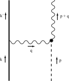
Figure 1: Feynman diagram for axion induced electric dipole moment. Solid dot is the axion anomaly interaction, $\theta\overrightarrow{E}\cdot\overrightarrow{B}$. The dashed line is the incoming axion field, $\theta$. The solid line is the electron, where the electron-photon vertex is the magnetic dipole moment operator of the electron.

The axion induced magnetic moment of the electron is about two orders of magnitude larger than that of the nucleon. Since the current best limit upon any DC elementary particle EDM is that of the electron, of order $d_{e}\leq 8.7\times 10^{-29}$ e-cm, ACME , the electron may be a promising place to search for an oscillating EDM and the axion itself.

II Feynman Diagram Analysis of Induced OEDM of the Electron

II.1 Nonrelativistic Pauli-Schroedinger Action

We compute the axion induced OEDM of the electron. We go to the electron rest frame which we assume to also be the rest frame of the cosmic axion field, i.e., the frame in which the axion field oscillates in time with no spatial dependence, $a/f=\theta_{0}\cos(m_{a}t)$. We use the Pauli-Schroedinger formalism, then follow with an analysis in Georgi’s heavy fermion formalism.

The Pauli-Schroedinger Lagrangian is, of course, the first order Dirac action in an expansion in $1/m_{e}$, and takes the form:

$$\frac{1}{2m}\psi^{\dagger}\overrightarrow{\sigma}\cdot\left(i\overrightarrow{\partial}-e\overrightarrow{A}\right)\overrightarrow{\sigma}\cdot\left(i\overrightarrow{\partial}-e\overrightarrow{A}\right)\psi$$ (4)

where $\psi$ is a two-component spinor. Eq.(4) contains the term:

$$-\frac{1}{2m}\psi^{\dagger}\overrightarrow{\sigma}\cdot\left(i\overrightarrow{\partial}\right)\overrightarrow{\sigma}\cdot\left(e\overrightarrow{A}\right)\psi\supset-\frac{ie}{2m}\psi^{\dagger}\epsilon_{ijk}\sigma_{k}\psi\partial_{i}A_{j}$$

having used $\sigma_{i}\sigma_{j}=\delta_{ij}+i\epsilon_{ijk}\sigma_{k}$. This is the standard magnetic dipole interaction, $-\frac{ige}{2m}\psi^{\dagger}\frac{\vec{\sigma}}{2}\psi\cdot\vec{B}$ with $g=2$.

Consider the time-ordered product of $i\times$ the magnetic dipole action with $i\times$ the axion anomaly action:

$$\!\!\!\!\!\!\!\!\!\!\!\!\!\!\!\!\!\!-(i)^{2}T\;\int d^{4}x\frac{ie}{2m}\psi^{\dagger}\epsilon_{ijk}\partial_{i}A_{j}\sigma_{k}\psi\;\;\;$$

$$\qquad\qquad\times{\tiny\frac{g_{a}}{2}\tiny}\int d^{4}y\theta\epsilon^{\alpha\beta\gamma\rho}\partial_{\alpha}A_{\beta}\partial_{\gamma}A_{\rho}$$ (6)

Assuming $\theta$ has only time dependence, and integrating the anomaly by parts in time we have

$$iT\frac{eg_{a}}{4m}\!\!\int\!d^{4}x\>\psi^{\dagger}\epsilon_{ijk}\sigma_{k}\psi\partial_{i}A_{j}\!\!\int\!d^{4}y(\partial_{0}\theta)\epsilon_{lmn}A_{l}\partial_{m}A_{n}$$

Note that this forces us into radiation gauge, as a Coulomb term would be $\sim\theta\epsilon_{lmn}\partial_{l}\phi\partial_{m}A_{n}$ and upon integration by parts we would have $\sim-\partial_{l}\theta\epsilon_{lmn}\phi\partial_{m}A_{n}$, which vanishes by the hypothesis that the axion field depends only upon time.

Contracting the vector potential from the magnetic dipole interaction with either vector potential in the anomaly yields:

$$\!\!\!\!\!\!\!\!\frac{eg_{a}}{2m}\int d^{4}y\int d^{4}x\;\psi(x)^{\dagger}\epsilon_{ijk}\sigma_{k}\psi(x)$$

$$\qquad\qquad\times\partial_{i}G(x-y)\partial_{0}\theta(y^{0})\epsilon_{jmn}\partial_{m}A_{n}(y)$$ (8)

where we’ve included a $2\times$ combinatorial factor. Here we use the covariant Feynman propagator of the photon,

$$i\left(g_{\mu\nu}-\lambda\frac{\partial_{\mu}\partial_{\nu}}{\partial^{2}}\right)G(x-y) \rightarrow -i\delta_{ij}G(x-y);$$

$$G(x-y)=-\int\frac{d^{4}k}{(2\pi)^{4}} \!\!\!\!\!\!\!\!\frac{e^{ik\cdot(x-y)}}{k^{2}+i\epsilon}$$ (9)

since only the spatial terms are relevant and the gauge dependent terms, $\propto\lambda$, are seen to cancel owing to antisymmetries (see ref.Hill1 ). Our sign conventions and normalization are consistent with ref.BjDrell , where we have $\partial^{2}G(x-y)=\delta^{4}(x-y)$.

Using, $\epsilon_{ijk}\epsilon_{jmn}=-\delta_{im}\delta_{kn}+\delta_{in}\delta_{km}$, we can write:

$$=-\frac{eg_{a}}{2m}\int d^{4}y\int d^{4}x\;\psi^{\dagger}\sigma_{k}\psi(x)$$

$$\qquad\qquad\times\;\partial_{i}G(x-y)\partial_{0}\theta(y^{0})\left(\partial_{i}A_{k}(y)-\partial_{k}A_{i}(y)\right)$$

Note that the result of eq.(II.1) is manifestly proportional to $\partial_{0}\theta$ and therefore the axion is derivatively coupled up a total divergence. However, when displayed in this form we do not see the manifest gauge invariance. This issue is addressed in detail in Section III.

We assume that the electron is in a common rest frame with the axion. To a good approximation the electron operator is static, i.e., $\partial_{0}(\psi^{\dagger}\sigma_{k}\psi)=0+O(1/m)$. since the electron mass is enormous compared to the relevant momentum exchange, $m_{e}>>m_{a}$. The electron can therefore absorb this tiny momentum without appreciably changing its energy.

We can therefore integrate the time derivative by parts, and drop $\partial_{y^{0}}G(x-y)$ terms. We can also integrate the spatial derivative $\partial_{y_{k}}$ by parts, and note the translational invariance of the propagator implies, $\partial_{y}G(x-y)=-\partial_{x}G(x-y)$. This yields:

$$=\frac{eg_{a}}{2m}\int d^{4}y\int d^{4}x\;\psi^{\dagger}\sigma_{k}\psi(x)\nabla_{x}^{2}G(x-y)\theta\left(\partial_{0}A_{k}(y)\right)$$

$$-\frac{eg_{a}}{2m}\int d^{4}y\int d^{4}x\;\psi^{\dagger}\sigma_{k}\psi(x)\partial_{k}G(x-y)\theta\left(\partial_{i}\partial_{0}A_{i}(y)\right)$$

where $\nabla^{2}=\partial_{k}\partial_{k}$. Using the definition of the electric field in radiation gauge, $E_{i}=-\partial_{0}A_{i}$, the static electron field permits us to integrate over $x^{0}$, $\int dx^{0}\;\nabla^{2}G(x-y)=\delta^{3}(x-y)$. We obtain the effective action (we have removed the $i$):

$$=\frac{ieg_{a}}{2m}\left[\int d^{4}x\;\psi^{\dagger}\sigma_{k}\psi\;\theta(t)E_{k}(x)\right.$$

$$\;\;\;\left.+\int d^{4}y\int d^{4}x\;\partial_{k}\psi^{\dagger}\sigma_{k}\psi(x)\ G(x-y)\theta(y^{0})\partial_{i}E_{i}(y)\right]$$

The result we have obtained contains the local contact interaction, which is a conventional electric dipole form proportional to $\theta(t)$. It also contains a nonlocal component. If we choose to immerse the electron in a source free field, such as an RF cavity mode or light, then $\partial_{i}E_{i}(y)=0$ and only the contact term remains.

We have written this expression in a manifestly gauge invariant form, and therefore we display the axion field without a derivative. Integration by parts, as in the general argument of Section III, shows that the axion is derivatively coupled. Our interaction behaves like the anomaly itself in its display of manifest gauge invariance vs manifest shift invariance..

II.2 Georgi’s Heavy Quark Effective Theory Applied to the Electron

The previous analysis relied upon the non-recoil approximation of the electron, which is justified since $m_{e}>>m_{a}$. This limit implies that the $4$-velocity of the electron is approximately conserved in its interactions with the comoving axion field. A more “covariant” representation can be derived, however, by using Georgi’s heavy quark effective field theory formalism georgi . We obtain the same basic structure as in the Pauli-Schroedinger case, but formulae involving the electric dipole moment will become the more familiar relativistic forms.

We begin by defining heavy electron Dirac fields with fixed 4-velocity, $v_{\mu}$:

$$\psi\rightarrow\left(\frac{1+v\!\!\!/\!\,\,}{2}\right)\psi=\psi_{v}\qquad\overline{\psi}\rightarrow\overline{\psi}\left(\frac{1+v\!\!\!/\!\,\,}{2}\right)=\overline{\psi}_{v}$$ (13)

The Dirac magnetic moment operator then takes the form:

$$-\frac{ie}{4m}\overline{\psi}_{v}\sigma_{\mu\nu}\psi_{v}F^{\mu\nu}=-\frac{ie}{2m}\overline{\psi}_{v}\left(\gamma_{5}\epsilon_{\alpha\beta\rho\gamma}\gamma^{\rho}v^{\gamma}\right)\psi_{v}\partial^{\alpha}A^{\beta}$$ (14)

where the axion field is $\theta=\theta_{0}\cos(m_{a}v_{\mu}x^{\mu})$.

We again compute the time ordered product of $i\times$ the magnetic dipole action with $i\times$ the axion anomaly action:

$$-(i)^{2}T\;\frac{ieg_{a}}{4m}\int d^{4}x\overline{\psi}_{v}(x)\left(\gamma_{5}\epsilon_{\alpha\beta\rho\gamma}\gamma^{\rho}v^{\gamma}\right)\psi_{v}(x)\partial^{\alpha}A^{\beta}(x)\;$$

$$\qquad\times\int d^{4}y\theta(y)\epsilon^{\eta\kappa\omega\rho}\partial_{\eta}A_{\kappa}(y)\partial_{\omega}A_{\rho}(y)$$

$$=-\frac{eg_{a}}{2m}\int d^{4}y\int d^{4}x\overline{\psi}_{v}(x)\left(\gamma_{5}\epsilon_{\alpha\beta\rho\gamma}\gamma^{\rho}v^{\gamma}\right)\psi_{v}(x)$$

$$\qquad\;\;\;\times\partial^{\alpha}G(x-y)\left(\partial_{\eta}\theta(y)\epsilon^{\eta\beta\omega\rho}\partial_{\omega}A_{\rho}(y)\right)$$ (15)

Note again that propagator gauge terms do not contribute owing the the $\epsilon$-symbols. We now relabel, permute, and use the identities:

$$\epsilon_{\alpha\beta\gamma\rho}\epsilon^{\alpha\eta\omega\delta}=-\left(g_{\beta}^{\eta}g_{\gamma}^{\omega}g_{\rho}^{\delta}+(-1)^{p}(\makebox{permutations})\right)$$ (16)

and:

$$-i\overline{\psi}_{v}\gamma^{5}\sigma_{\alpha\beta}{\psi}_{v}=\overline{\psi}_{v}\left(\gamma^{5}\gamma_{\alpha}v_{\beta}-\gamma^{5}\gamma_{\beta}v_{\alpha}\right){\psi}_{v}$$ (17)

Note that we can integrate by parts and rearrange, to obtain:

$$\!\!\!\!\!\!\!\!\!\!\!\!=\frac{ieg_{a}}{2m}\int d^{4}y\int d^{4}x\;\overline{\psi}_{v}\gamma_{5}\sigma^{\rho\gamma}\psi_{v}\left[\partial^{2}G(x-y)(\partial_{\rho}\theta)A_{\gamma}\right.$$

$$\left.\qquad+\partial^{\beta}\partial_{\gamma}G(x-y)\left((\partial_{\beta}\theta)A_{\rho}-(\partial_{\rho}\theta)A_{\beta}\right)\right]$$ (18)

This form displays the manifest derivative coupling of the axion, but not manifest gauge invariance.

Alternatively, we can manipulate eq.(II.2), using $\partial^{2}G(x)=\delta^{4}(x)$, and multiplying by $-i$ to obtain the action:

$$\!\!\!\!\!\!\!\!\!\!\!\!\!\!\!\!\!\!\!\!=-\frac{eg_{a}}{4m}\int d^{4}x\;\overline{\psi}_{v}\left(\gamma_{5}\sigma_{\rho\gamma}\right)\psi_{v}\theta F^{\rho\gamma}$$

$$\!\!\!\!\!\!\!\!\!\!\!\!\!\!\!-\;\frac{eg_{a}}{2m}\int\!d^{4}y\int\!d^{4}x\;\partial^{\rho}(\overline{\psi}_{v}\left(\gamma_{5}\sigma_{\rho\gamma}\right)\psi_{v}(x))$$

$$\qquad\qquad\;\;\;\times G(x-y)\partial_{\beta}[\theta(y)F^{\gamma\beta}(y)]$$ (19)

Here we have displayed manifest gauge invariance, while the derivative coupling of the axion is not manifest. We emphasize that eq.(II.2) and eq.(II.2) are equivalent up to surface terms. Note that in eq.(II.2) we see the familiar covariant EDM operators in the heavy quark fields: $\overline{\psi}_{v}\left(\gamma_{5}\sigma_{\rho\gamma}\right)\psi_{v}(x)$ .

To compare the Georgi calculation result to the Pauli-Schroedinger case we go to rest frame $v_{i}\rightarrow 0$, and carefully note sign conventions in ref.BjDrell :

$$-\frac{eg_{a}}{4m}\int d^{4}x\overline{\psi}_{v}\gamma^{5}\sigma_{\alpha\beta}\psi_{v}\left(\theta F^{\alpha\beta}\right)$$

$$\rightarrow\frac{ieg_{a}}{2m}\int d^{4}x{\psi}^{\dagger}\sigma_{i}\psi\left(\theta E_{i}\right)$$ (20)

and:

$$\!\!\!\!\!\!\!\!\!\!-\frac{eg_{a}}{2m}\int d^{4}y\int d^{4}x\partial^{\beta}\overline{\psi}_{v}\left(\gamma_{5}\sigma_{\beta\rho}\right)\psi_{v}\cdot$$

$$\qquad\qquad\qquad G(x-y)\partial_{\gamma}[\theta(y)F^{\rho\gamma}(y)]$$

$$\rightarrow\frac{ieg_{a}}{2m}\int d^{4}y\int d^{4}x\;\partial_{i}\left(\overline{\psi}^{\dagger}\sigma_{i}\psi(x)\right)$$

$$\qquad\qquad\qquad G(x-y)\cdot\left(\theta\partial_{j}E_{j}(y)\right)$$ (21)

where the latter spinors (without subscript, _v) are two-component spinors. These expressions are equivalent to eq.(II.1). The result of eq.(II.2) is somewhat more general than eq.(II.1), the latter refering to the frame with electron and axion both having $4$-velocity $v_{\mu}$.

III Anomalies, OEDM’s, and Axion Decoupling

III.1 The General Form of the Action

Presently we give a general argument as to why the nonlocal term occurs, and we will derive the general structure of the action by simply demanding the shift-symmetry of the axion.

The effect we are discussing arises perturbatively, from the interaction of the axion anomaly with a magnetic moment and therefore it must share subtleties with the anomaly itself. The anomalous interaction of the axion with electromagnetic fields is written in eq.(2):

$$\frac{g_{a}}{2}\epsilon_{\mu\nu\rho\sigma}\int d^{4}x\;\theta(x)F^{\mu\nu}{F}^{\rho\sigma}$$ (22)

where $\theta(x)=a(x)/f_{a}$ .

We can perform a transformation that shifts the axion as $\theta\rightarrow\theta+\phi$ where $\phi$ is an arbitrary angle. If $\phi$ is constant the theory is invariant under this shift, since the anomaly only causes the action of eq.(22) to shift by a total divergence, which has no effect in perturbation theory (a total divergence, or “surface term,” is $\propto$ the total incoming momentum less the total outgoing momentum of the Feynman diagram). Therefore, we conclude, $a/f_{a}$ must be derivatively coupled in any perturbative process.

We see this in eq.(22) if we integrate by parts and write:

$$-g_{a}\epsilon_{\mu\nu\rho\sigma}\int d^{4}x\;\partial^{\mu}\theta(t)A^{\nu}{F}^{\rho\sigma}$$ (23)

where $A_{\mu}$ is the vector potential, and ${F}_{\mu\nu}=\partial_{\mu}A_{\nu}-\partial_{\nu}A_{\mu}$. Eq.(23) displays the derivative coupling of the axion, however the manifest gauge invariance of electromagnetism is lost. Alternatively, eq.(22) maintains the gauge invariance of QED, but does not display the $U(1)_{PQ}$ “shift” symmetry of the pNGB. Both symmetries are present in perturbation theory since eq.(22) and eq.(23) differ only by surface terms. We observed in Section II that this feature is shared by the Feynman diagram that generates a perturbatively induced OEDM.

We generally define the covariant OEDM of the electron (or similarly for any other object) in an arbitrary frame in which the cosmic axion field has four-velocity $u_{\mu}$, i.e., $\theta(x)=\theta_{0}\cos(u_{\mu}x^{\mu})$, as:

$$S^{\prime}=g^{\prime}\int d^{4}x\;\theta(x)S_{\mu\nu}F^{\mu\nu}$$ (24)

where $S_{\mu\nu}$ is an antisymmetric odd parity dipole density ($S^{0}_{\mu\nu}\sim\overline{\psi}\sigma_{\mu\nu}\gamma^{5}\psi$; $S_{\mu\nu}$ will be defined in terms of $S^{0}_{\mu\nu}$ momentarily).

Since this result arises perturbatively from the anomaly, it must have the shift symmetry in common with the anomaly. In particular we must be able to move a derivative exclusively onto $\theta$ via integration by parts:

$$S^{\prime}=-2g^{\prime}\int d^{4}x\;\partial^{\mu}\theta(x)S_{\mu\nu}A^{\nu}$$ (25)

We see that the gauge field, $A^{\mu}$, now appears explicitly, exactly as happens in the case of the anomaly itself.

However, in order for eq.(25) to be valid, a constraint must be satisfied:

$$\partial^{\mu}S_{\mu\nu}=0$$ (26)

A general solution to this constraint can be written as a nonlocal form:

$$S_{\mu\nu}=S^{0}_{\mu\nu}(x)+\int d^{4}y\;\partial_{[\mu}G(x-y)\partial^{\lambda}S^{0}_{\nu]\lambda}(y)$$ (27)

(note antisymmetrization in $\mu$ and $\nu$). Eq.(26) satisfies $\partial^{\mu}S_{\mu\nu}=0$ for any antisymmetric $S^{0}_{\mu\nu}$, where the Green’s function satisfies:

$$\partial^{2}G(x-y)=\delta^{4}(x-y)$$ (28)

and $G(x-y)$ is as defined in eq.(II.1).

The action with eq.(27) thus becomes;

$$S^{\prime} = g^{\prime}\int d^{4}x\;d^{4}y\;\theta(x)F^{\mu\nu}(x)$$ (29)

$$\!\!\!\!\!\!\!\!\!\!\times\left[S^{0}_{\mu\nu}(x)\delta^{4}(x-y)+\partial_{[\mu}G(x-y)\partial^{\lambda}S^{0}_{\nu]\lambda}(y)\right]$$

and $S^{0}_{\mu\nu}=\overline{\psi}\sigma_{\mu\nu}\gamma^{5}\psi$ is local. We can transpose the integrand, using $\partial_{x}G(x-y)=-\partial_{y}G(x-y)$ and performing integrations by parts in $y$, to obtain:

$$S^{\prime} = g^{\prime}\int d^{4}x\;\theta(x)S^{0}_{\mu\nu}(x)F^{\mu\nu}$$ (30)

$$\!\!\!\!\!\!\!\!\!\!\!\!\!\!\!\!\!\!\!\!\!\!\!\!\!+2\int d^{4}x\int d^{4}y\;S^{0}_{\rho\nu}(x)G(x-y)\partial^{\rho}\partial^{[\mu}(\theta(y)F_{\mu}^{\;\;\nu]}(y))$$

This is seen to be equivalent, e.g., to the Georgi formalism result of eq.(II.2) after an integration by parts, where we have $g^{\prime}=eg_{a}/4m$ and $S^{0}_{\mu\nu}=\overline{\psi}_{v}\gamma_{5}\sigma_{\mu\nu}\psi_{v}$. The role of the nonlocal term is therefore to maintain the shift symmetry of the axion.

The nonlocal term reduces further in certian limits. In the limit of a constant $\theta(x)$ we have $\partial^{\mu}(\theta(y)F_{\mu}^{\;\;\nu}(y))=\theta\partial^{\mu}F_{\mu}^{\;\;\nu}(y)=j^{\;\;\nu}(y)$, where $j^{\nu}(y)$ is a source current for the electromagnetic field. Since $\partial^{2}G=\delta$, the vector potential is given by:

$$A_{\mu}(x)=\int d^{4}y\;G(x-y)j_{\mu}(y)$$ (31)

Hence, for constant $\theta$:

$$S^{\prime}\rightarrow\int\theta S_{\mu\nu}F^{\mu\nu}-\int\theta S_{\mu\nu}F^{\mu\nu}=0$$ (32)

which is the simplest statement of decoupling.

We can also consider a static limit for the electron in which:

$$\int dy^{0}\;G(x-y) = \int\frac{d^{3}\vec{k}}{(2\pi)^{3}}\frac{e^{-i\vec{k}\cdot(\vec{x}-\vec{y})}}{\vec{k}^{2}}$$ (33)

$$= \frac{1}{4\pi}\frac{1}{|\vec{x}-\vec{y}|}\equiv-\frac{1}{\vec{\nabla}^{2}}$$

where $\vec{\nabla}^{2}(1/R)=-4\pi\delta^{3}(R)$ (e.g, see Jackson section 6.4). We find by explicit calculation of Fig.(1) that $S^{0}_{\mu\nu}$ is the a local electric dipole density operator, $\propto i\overline{\psi}\gamma^{5}\sigma_{\mu\nu}\psi$).

For a purely spatially constant but time dependent axion field, $\theta(t)$ and a nonrelativistic, static electric dipole moment, $g^{\prime}S^{0}_{0i}=-g^{\prime}S^{0}_{i0}=\frac{1}{2}{P}_{i}(x)$, where $\partial_{t}{P}_{i}(x)=0$ this becomes:

$$\small S^{\prime}=g^{\prime}\int d^{4}x\;\theta(t)\left(\overrightarrow{P}\cdot\overrightarrow{E}+\overrightarrow{\nabla}\cdot\overrightarrow{P}\left(\frac{1}{\overrightarrow{\nabla}^{2}}\right)\overrightarrow{\nabla}\cdot\overrightarrow{E}\right)$$ (34)

In an arbitrary gauge, $\overrightarrow{E}=\overrightarrow{\nabla}\varphi-\partial_{t}\overrightarrow{A}$ , we see that:

$$S^{\prime}=g^{\prime}\int d^{4}x\;\theta(t)\overrightarrow{\nabla}\cdot(\overrightarrow{P}\varphi)$$

$$\!\!\!\!\!\!\!\!+g^{\prime}\int d^{4}x\;\partial_{t}\theta(t)\left(\overrightarrow{P}\cdot\overrightarrow{A}+\overrightarrow{\nabla}\cdot\overrightarrow{P}\left(\frac{1}{\overrightarrow{\nabla}^{2}}\right)\overrightarrow{\nabla}\cdot\overrightarrow{A}\right)$$ (35)

Therefore, $S^{\prime}$ becomes a total divergence in the limit $\partial_{t}\theta(t)\rightarrow 0.$ In particular, the first term is a total divergence in space for a spatially constant $\theta(t)$.

In the case of a source-free electric field, $\nabla\cdot\vec{E}=0$, this becomes:

$$g^{\prime}\int d^{4}x\;\theta(t)\overrightarrow{P}\cdot\overrightarrow{E}$$ (36)

indistinguishable from a simple electric dipole moment interaction. Because $\overrightarrow{E}=-\partial_{t}\vec{A}$, we can integrate this expression by parts to write:

$$g^{\prime}\int d^{4}x\;\partial_{t}\theta(t)\overrightarrow{P}\cdot\overrightarrow{A}$$ (37)

and manifest gauge invariance is lost, just as in the case of the anomaly when the derivative is placed on the axion field. Eqs.(36) and (37) differ only by surface terms that are irrelevant to perturbation theory.

Note that if the electric field has a static source, such as an electric charge (e.g., an atomic nucleus), located at $\vec{x}_{0}$, $\overrightarrow{\nabla}\cdot\overrightarrow{E}(y)=Q\delta^{3}(\vec{y}-\vec{x})$ and, ignoring the explicit $\partial_{t}\theta\sim m_{a}$ terms in the nonlocal component of eq.(30), then quasistatic action reduces to:

$$g^{\prime}\int d^{4}x\;(\theta(t)-\theta(t-|\vec{x}-\vec{x}_{0}|)\overrightarrow{P}(x)\cdot\overrightarrow{E}(x)$$ (38)

Here we see that the nonlocal term subtracts a retarded axion field from the local value of the axion field. This difference vanishes as $m_{a}\rightarrow 0$. This is the way the decoupling is generally maintained in solutions to Maxwell’s equations in classical configurations, such as RF cavities, as we see in the next few sections. This result, however, implies that the electron OEDM may be difficult to probe in atomic experiments (such as the ACME experiment, ACME ) where $|\vec{x}-\vec{x}_{0}|\sim r_{Bohr}$ is the Bohr radius, since $(\theta(t)-\theta(t-|\vec{x}-\vec{x}_{0}|)\sim m_{a}r_{Bohr}<<1$.

We emphasize that a nonlocal operator structure in electrodynamics is not novel. It is encountered in the “transverse electromagnetic current” in QED, e.g., when we quantize in radiation gauge (see, eg, Jackson , section 6.3 and eq.(6.28)). In that case the nonlocal term is essential to maintain the causality of the theory in this gauge. The transverse current occurs when we have Coulombic sources and a nonzero, time dependent component of the vector potantial, $A_{0}$. $A_{0}$ has no time derivatives in the action and is therefore an instantaneously propagating field, and cannot represent a physical out-going on-shell photon. The equation of motion for $A_{0}$ is $\vec{\nabla}^{2}A_{0}=-\rho(x)$, where $\rho(x)$ is a charge density. If we want to allow time dependent $A_{0}$, then $\nabla^{2}\partial_{0}A_{0}=-\partial_{0}\rho(x,t)$, but from current conservation we have $\partial_{0}\rho=\nabla\cdot\vec{j}$ where $\vec{j}$ is the 3-current. Hence, we have $\partial_{0}A_{0}=-(1/\vec{\nabla}^{2})\vec{\nabla}\cdot\vec{j}$. This means that if $A_{0}$ is to be time dependent, then there must necessarily be a 3-current, hence a vector potential, $\vec{A}$. We impose the condition $\vec{\nabla}\cdot\vec{A}=0$. $\vec{A}$ satisfies $(\partial_{0}^{2}-\nabla^{2})\vec{A}-\vec{\nabla}\partial_{0}A_{0}=\vec{j}$ (the equation of motion of $A_{0}$ is unmodified by this). This is often written as $(\partial_{0}^{2}-\nabla^{2})\vec{A}=\vec{j}_{T}$. where $\vec{j}_{T}$ is the “transverse current” Jackson which takes the form $\vec{j}_{T}=\vec{j}-\vec{\nabla}(1/\nabla^{2})\vec{\nabla}\cdot\vec{j}$. $\vec{j}_{T}$ is identically conserved with the nonlocal term, is consistent with the radiation gauge condition $\vec{\nabla}\cdot\vec{A}=0$, and thus gauge invariance is maintained. From this, Lorentz invariance is also maintained.

Thus, introducing $A_{0}$ time dependence requires a nonlocal correction to the current to maintain a conserved current, hence gauge invariance. This is formally similar to the structure seen in eq.(27) which maintains the shift symmetry (analogue of gauge symmetry) of the axion. The apparent nonlocality is arising because we are treating the “vacuum” as effectively containing a space-time dependence, through the background cosmic classical $\theta(t)$ field. Physical amplitudes thus inherit a nonlocal dependence upon the history of the vacuum.

III.2 Axion in an Infinite Volume Static Magnetic Field and Inherent Nonlocality

The “integral form of axion decoupling,” as we have seen above arising from the nonlocal term, is a general feature of the solutions to the Maxwell equations in various practical situations. Suppose we have an infinite universe which contains a uniform static magnetic field $\overrightarrow{B}_{0}$ and a background oscillating classical axion field, $a(t)/f\equiv\theta\left(t\right)=\theta_{0}\cos\left(m_{a}t\right)$ (this can be considered as an infinite volume limit of an RF cavity experiment as we do below). We consider the sources for $\overrightarrow{B}_{0}$ to be far away from the region of interest and therefore $\overrightarrow{\nabla}\times\overrightarrow{B}_{0}=0$. The decoupling, $m_{a}\rightarrow 0$ limit, becomes somewhat subtle, even in this case. We can analyze this classically.

The axion anomaly will generate an electromagnetic field of the form: $\overrightarrow{E}=\overrightarrow{E}_{r}$ and $\overrightarrow{B}=\overrightarrow{B}_{0}+\overrightarrow{B}_{r}$ where $\overrightarrow{E}_{r}$ and $\overrightarrow{B}_{r}$ are oscillating “response fields.” Maxwell’s Equations in these fields become:

Maxwell (1):

$$\qquad\overrightarrow{\nabla}\times\overrightarrow{B}_{r}-\partial_{t}\overrightarrow{E}_{r}=-g_{a}\overrightarrow{B}_{0}\left(\partial_{t}\theta\right)$$ (39)

Maxwell (2)

$$\qquad\overrightarrow{\nabla}\times\overrightarrow{E}_{r}+\partial_{t}\overrightarrow{B}_{r}=0$$ (40)

and $\ \ \overrightarrow{\nabla}\cdot\overrightarrow{B}_{r}=\overrightarrow{\nabla}\cdot\overrightarrow{E}_{r}=0.$

The Maxwell equations are coupled first order inhomogeneous differential equations. They are consistent with the decoupling of the axion as $m_{a}\rightarrow 0$, since the source term is proportional to $\partial_{t}\theta$. The vector potential in Coulomb gauge likewise satisfies: $\partial_{t}^{2}\overrightarrow{A}_{r}-\overrightarrow{\nabla}^{2}\overrightarrow{A}_{r}=-g_{a}\overrightarrow{B}_{0}\left(\partial_{t}\theta\right)$  where  $\overrightarrow{E}_{r}=-\partial_{t}\overrightarrow{A}_{r}$ and $\nabla\cdot\overrightarrow{A}_{r}=0$, a single second order inhomogeneous differential equation. For an infinite universe filled with the magnetic field $\overrightarrow{B}_{0}$ we have translational invariance in space.

The Maxwell equations have a particular solution that is consistent with the symmetry of spatial translational invariance:

$$\overrightarrow{E}_{r} = g_{a}\overrightarrow{B}_{0}\int_{0}^{t}d\tau\partial_{\tau}\theta(\tau)=g_{a}\overrightarrow{B}_{0}\left(\theta(t)-\theta(t_{0})\right)$$

$$\overrightarrow{B}_{r} = 0$$ (41)

The solutions necessarily require the specification of a single boundary condition at an inital time, which we take to be $\overrightarrow{E}_{r}(t_{0})=0$ and $\overrightarrow{B}_{r}(t_{0})=0$ . We emphasize that this is a non-propagating solution (since $\overrightarrow{B}_{r}=0$) and represents a time dependent “dual rotation” of $\overrightarrow{B}_{0}\rightarrow\overrightarrow{E}_{r}$ Hill1 .

The dependence upon the initial condition introduces an apparent nonlocality, or “history”, into the observed $\overrightarrow{E}_{r}(t)$. Clearly $\overrightarrow{\nabla}\times\overrightarrow{E}_{r}=0$ hence $B_{r}=0$. Note that the vector potential is nonlocal, satisfying

$$\overrightarrow{A}_{r}=g_{a}\overrightarrow{B}_{0}\int_{0}^{t}d\tau^{\prime}\int_{0}^{\tau^{\prime}}d\tau\partial_{\tau}\theta(\tau)$$ (42)

Our infinite universe with a static magnetic field and an oscillating axion field has acquired an oscillating electric field. This is an example of a general “theorem:” Any magnetic moment becomes an oscillating electric moment in the presence of the oscillating axion. The magnetic field need not be restricted to a constant all-space filling form as in this toy universe example; it can be, e.g., the local field surrounding a magnetic dipole moment, as we can see classically. The effect of the axion is to produce a time dependent electric dipole for the electron.

III.3 Axion Induced Electric Field in an RF Cavity

To detect a cosmic axion signal we can deploy a very large constant, externally applied magnetic field $\overrightarrow{B}_{0}$ within a resonant cavity. The solutions to the Maxwell equations for the response fields will always involve the same particular solution we just encountered in the toy universe, but also now includes homogeneous solutions that are required to implement the boundary conditions of the cavity.

Maxwell’s equations for the reponse fields are as in eqs.(39,40). We now have conducting boundary conditions at the cavity wall, $r=R$: $\overrightarrow{E}(r=R)=0$ (and since the form of the $B$-field is parallel to the cavity axis, we have no constraint upon $\overrightarrow{B}(r=R)$).

With cylindrical coordinates, ($\rho,\phi,z$ ), we find a cylindrically symmetric solution:

$$\overrightarrow{E} = \left(kJ_{0}(\rho m_{a})+g_{a}\right)B_{0}\widetilde{\theta}\widehat{z}$$

$$\overrightarrow{B} = kJ_{1}(\rho m_{a})B_{0}\frac{\partial_{t}\widetilde{\theta}}{m_{a}}\ \widehat{\phi}$$ (43)

The electric field has the form of our free space solution proportional to $g_{A}$, plus a homogeneous cavity mode solution proportional to $k.$

We now apply conducting boundary conditions at the cavity wall, $\ \overrightarrow{E}(\rho=R)=0$. We thus determine $k:$

$$\overrightarrow{E}=-g_{a}\left(\frac{J_{0}(\rho m_{a})}{J_{0}(Rm_{a})}-1\right)B_{0}\widehat{z}\widetilde{\theta}$$

$$\overrightarrow{B}=-g_{a}\frac{J_{1}(\rho m_{a})}{J_{0}(Rm_{a})}B_{0}\widehat{\phi}\left(\frac{\partial_{t}\widetilde{\theta}}{m_{a}}\right)$$ (44)

Note again that the solution vanishes as $m_{a}\rightarrow 0$ since we define $\widetilde{\theta}(t)=\int_{t_{0}}^{t}d\tau\partial_{\tau}\theta(\tau),$ where $t_{0}$ is an earlier time at which $\overrightarrow{E}(t_{0})=0$. The solutions is therefore intrinsically nonlocal in time. Henceforth we will omit the understood tilde on $\widetilde{\theta}$, i.e., $\theta\rightarrow\theta(t)-\theta(t_{0})$.

This is an idealized solution with a perfect resonant behavior, i.e., for a special cavity satisfying $J_{0}(Rm_{a})=0$ the solution has an apparent infinite amplitude. Of course, in reality the amplitude is damped by dissipation. This results in a finite $Q$ value, and modifies the solution to:

$$\overrightarrow{E} = -g_{a}\left(\frac{J_{0}(\rho m_{a})}{F}-1\right)B_{0}\widehat{z}{\theta}$$

$$\overrightarrow{B} = -g_{a}\frac{J_{1}(\rho m_{a})}{F}B_{0}\widehat{\phi}\left(\frac{\partial_{t}{\theta}}{m_{a}}\right)$$ (45)

where

$$F=\sqrt{\left(J_{0}(Rm_{a})\right)^{2}+1/Q^{2}}$$ (46)

Note that the total oscillating field energy in the cavity is $\propto Q^{2}$. The finite $Q$ arises if we include a resistive damping term in the Maxwell equations. In an idealized perfect cavity the oscillating fields are the electric field $90^{o}$ out of phase from the magnetic field, and hence a vanishing time averaged Poynting vector. There is, however, with finite $Q$ there is an induced, small ${\cal{O}}(1/Q)$, temporal phase shift, that we have not written, such that $\overrightarrow{E}$ and $\overrightarrow{B}$ are not exactly $90^{o}$ out of phase. This allows the Poynting vector at the walls of the cavity to average to a nonzero result. Hence power is extracable at a rate $\propto Q$. If we attempt to extract power at faster rate then $Q$ will decrease since the dominant power loss mechanism becomes the radiative extraction itself. We will consider some quantitative aspects of the RF cavity solution in Section V.

IV Electric Dipole Radiation from a Stationary Electron

IV.1 Classical Calculation

First we consider the electric dipole radiation from a classical magnetic moment immersed in the axion field. This calculation has validity for intense classical magnetic sources. It cannot be adapted to the case of an electron which requires the quantum calculation. Nonetheless, it is instructive to compute and compare it with the quantum case in Section IV.B. We will see that the radiation is generated by the physical OEDM. The magnetic dipole field surrounding the source, though it appears on the rhs of Maxwell’s equations as a source term in the axion background, does not itself radiate. Instead, this is associated with the non-radiating particular solution encountered in the previous section, and it allows implementation of various boundary conditions at short distance for the electric field.

The standard Maxwell equations with axion anomaly source in the presence of an arbitrary static, local magnetic field $\overrightarrow{B}_{0}(\vec{r})$ are:

Maxwell (1):

$$\qquad\overrightarrow{\nabla}\times\overrightarrow{B}_{r}(\vec{r},t)-\partial_{t}\overrightarrow{E}_{r}(\vec{r},t)=-g_{a}\overrightarrow{B}_{0}(\vec{r})\partial_{t}\theta(t)$$ (47)

Maxwell (2)

$$\qquad\overrightarrow{\nabla}\times\overrightarrow{E}_{r}(\vec{r},t)+\partial_{t}\overrightarrow{B}_{r}(\vec{r},t)=0$$ (48)

and $\overrightarrow{\nabla}\cdot\overrightarrow{B}_{r}=\overrightarrow{\nabla}\cdot\overrightarrow{E}_{r}=0.$

Presently $\overrightarrow{B}_{0}(\vec{r})\equiv\overrightarrow{\nabla}\times\overrightarrow{A}_{0}(\vec{r})$ will be the static field of a classical solenoidal magnet, centered at the origin, $\vec{r}=0$, where $\overrightarrow{A}_{0}$ can be written formally in terms of a magnetic dipole source $\overrightarrow{m}_{0}=\overrightarrow{m}\delta^{3}(\overrightarrow{r})$, (see ref.Jackson , Chapter 5.6). We have formally:

$$-\overrightarrow{\nabla}\times\overrightarrow{B}_{0}=\overrightarrow{\nabla}^{2}\overrightarrow{A}_{0}=\overrightarrow{\nabla}\times\overrightarrow{m}_{0}$$ (49)

hence:

$$\overrightarrow{A}_{0}=\frac{1}{4\pi}\frac{\overrightarrow{m}\times\overrightarrow{r}}{r^{3}}$$ (50)

and:

$$\overrightarrow{B}_{0}=-\frac{1}{4\pi}\left[\frac{8\pi}{3}\overrightarrow{m}\delta^{3}(\vec{r})+\left(\frac{1}{r^{3}}\right)\left(\overrightarrow{m}-\frac{3\overrightarrow{r}\left(\overrightarrow{r}\cdot\overrightarrow{m}\right)}{r^{2}}\right)\right]$$ (51)

(see the magnetostatics discussion in Jackson, eqs.(5.55-5.64) Jackson ; Jackson states that this is a purely classical construction and cannot be unambiguously applied to a quantum mechanical electron).

A subtlety arises in the present case with the particular solution encountered in Section III. Consider a “sourceless dipole field,” i.e., one in which there is no $\overrightarrow{m}\delta^{3}(\vec{r})$ term:

$$\widehat{B}_{0}=-\frac{1}{4\pi}\left(\frac{1}{r^{3}}\right)\left(\overrightarrow{m}-\frac{3\overrightarrow{r}\left(\overrightarrow{r}\cdot\overrightarrow{m}\right)}{r^{2}}\right)$$ (52)

We consider Maxwell’s equations, replacing $\overrightarrow{B}_{0}$ by $\widehat{B}_{0}$ on the rhs of eq.(47). We then have the particular solution to the vacuum Maxwell equations:

$$\ \overrightarrow{E}_{r}(\vec{r},t) = -g_{a}\widehat{B}_{0}(\vec{r})\theta(t)$$ (53)

and:

$$\overrightarrow{B}_{r}(\vec{r},t)=0$$ (54)

This is a solution since:

$$0=\overrightarrow{\nabla}\times\left(\frac{\overrightarrow{m}}{r^{3}}-3\frac{\overrightarrow{r}\left(\overrightarrow{m}\cdot\;\overrightarrow{r}\right)}{r^{5}}\right)$$ (55)

(note that any potential severe surface term singularity arising here, e.g., such as in $\overrightarrow{\nabla}_{i}(r_{j}/r^{5})$, will be $\propto\delta_{ij}$ or $\propto r_{i}r_{j}$, but contracted with $\epsilon_{ijk}$ from the cross-product, and hence zero). However, since $\overrightarrow{B}_{r}(\vec{r},t)=0$, this is a nonpropagating solution. It exists for any background static magnetic field satisfying $\overrightarrow{\nabla}\times\overrightarrow{B}_{0}=0$ . We will require incorporating this non-propagating solution into our full radiation solution momentarily.

The existence of this solution has an important implication: The sourceless dipole field surrounding the origin, does not lead to radiation. The radiation comes only when we have a nonzero magnetic field $\overrightarrow{B}_{0}$ which curls around a nonzero dipole source term. This is analogous to the infinite universe with a constant magnetic field versus the RF cavity: it is the conducting wall of the cavity that enforces the boundary condition that produces the resonant magnetic and electric fields.

We can now solve the Maxwell equations using retarded Green’s functions for a vector potential, $A_{r}(\vec{r},t)$, describing the radiative oscillating response fields in Coulomb gauge. The analysis mostly follows the textbook derivations as in Jackson , Chapter 9, but involves the non-propagating solution described above. In what follows, we will pass to complex notation where $\theta(t)=\theta_{0}\exp(im_{a}t)$, and the physical response fields will be the real parts of the complex $\overrightarrow{E}_{r}$ and $\overrightarrow{B}_{r}$. The radiated electromagnetic fields $\overrightarrow{B}_{r}(\vec{r},t)$ and $\overrightarrow{E}_{r}(\vec{r},t)$ are obtained as follows:

$$\ \overrightarrow{E}_{r}(\vec{r},t) = -\frac{1}{4\pi}g_{a}\theta(t)\exp(-im_{a}|\overrightarrow{r}|)$$ (56)

$$\!\!\!\!\!\!\!\!\!\!\!\!\!\!\!\!\!\!\!\!\!\!\!\!\!\!\!\!\!\!\!\!\!\!\!\!\!\!\!\!\cdot\left(\left[1-\exp(im_{a}|\overrightarrow{r}|)+im_{a}r\right]\left(\frac{\overrightarrow{m}}{r^{3}}-3\frac{\overrightarrow{r}\left(\overrightarrow{m}\cdot\;\overrightarrow{r}\right)}{r^{5}}\right)\right.$$

$$\left.\qquad-m_{a}^{2}\left(\frac{\overrightarrow{m}}{r}-\frac{\overrightarrow{r}(\overrightarrow{m}\cdot\overrightarrow{r})}{r^{3}}\right)\right)$$

and:

$$\overrightarrow{B}_{r}(\vec{r},t)=\frac{1}{4\pi}g_{a}\partial_{t}\theta(t)\exp(-im_{a}|\overrightarrow{r}|)$$

$$\!\!\!\!\!\!\!\!\!\!\!\!\!\!\!\!\!\!\!\!\!\!\!\!\!\!\!\!\!\!\!\!\!\!\!\!\!\!\!\!\cdot\;\overrightarrow{m}\times\left(\frac{\overrightarrow{r}}{r^{3}}+\frac{im_{a}\overrightarrow{r}}{r^{2}}\right)$$

One can readily verify that eqs.(56, IV.1) satisfy the Maxwell equations eqs.(47, 48) with the source term $-g_{a}\overrightarrow{B}_{0}(\vec{r})\left(\partial_{t}\theta(t)\right)$. Notice that the second term in the brackets $\left[...\right]$ in eq.(56) is the non-propagating solution of eq.(53)

Taking the near-zone limit yields:

$$\overrightarrow{E}_{r}(\vec{r},t) \rightarrow 0$$ (58)

which vanishes due to cancellation with the particular solution, and:

$$\overrightarrow{B}_{r}(\vec{r},t)\rightarrow\frac{1}{4\pi}g_{a}im_{a}\theta(t)\left(\ \overrightarrow{m}\ \times\frac{\overrightarrow{r}}{r^{3}}\right)$$ (59)

From the near-zone limit we can confirm the Maxwell equations and read-off the source structure:

$$\nabla\times\overrightarrow{B}_{r}-\partial_{t}\overrightarrow{E}_{r} = -\frac{1}{4\pi}g_{a}\partial_{t}\theta(t)\left(-\frac{8\pi}{3}\overrightarrow{m}\delta^{3}(\overrightarrow{r})\right.$$ (60)

$$\qquad\left.+\frac{\overrightarrow{m}}{r^{3}}-3\frac{\overrightarrow{r}\text{ }\left(\overrightarrow{m}\cdot\overrightarrow{r}\right)}{r^{5}}\right)$$

Thus we see that the propagating radiation is due to the physical OEDM source, which induces the curling magnetic field, and is not due to the dipole magnetic field surrounding the source.

In the far-zone we have:

$$\overrightarrow{E}_{r}(\vec{r},t)\rightarrow\frac{g_{a}m_{a}^{2}}{4\pi}\theta(t)\exp(-im_{a}|\overrightarrow{r}|)\left(\frac{\overrightarrow{m}}{r}-\frac{\overrightarrow{r}}{r^{2}}\frac{\overrightarrow{m}\cdot\overrightarrow{r}}{r}\right)$$

$$\overrightarrow{B}_{r}(\vec{r},t)\rightarrow-\frac{g_{a}m_{a}^{2}}{4\pi}\theta(t)\exp(-im_{a}|\overrightarrow{r}|)\left(\ \overrightarrow{m}\ \times\left(\frac{\overrightarrow{r}}{r^{2}}\right)\right)$$

These are seen to be formally equivalent to the electric dipole radiation fields , where our magnetic moment $\vec{m}$ replaces the electric moment $\vec{p}$ in Jackson, Jackson eq.(9.18). Hence, the source of the radiation is the axion induced OEDM.

From this we can compute the cycle averaged Poynting vector, $\overrightarrow{K}=<\overrightarrow{E}_{r}\times\overrightarrow{B}_{r}>$:

$$\overrightarrow{K}=\frac{1}{32\pi^{2}}g_{a}^{2}m_{a}^{4}\theta_{0}^{2}\left[\left(\frac{\overrightarrow{r}}{r^{2}}\right)\left(\frac{\overrightarrow{m}^{2}}{r}-\frac{\left(\overrightarrow{m}\cdot\overrightarrow{r}\right)^{2}}{r^{3}}\right)\ \right]$$ (63)

Using $\overrightarrow{m}=\mu_{Bohr}\vec{S}$, the angular differential emitted power, $P$, for our classical electron is therefore given by the classical dipole pattern (Jackson , eq.(9.23)):

$$\frac{dP}{d\Omega}=\frac{1}{32\pi^{2}}g_{a}^{2}m_{a}^{4}\theta_{0}^{2}\mu_{\text{Bohr}}^{2}\sin^{2}\theta$$ (64)

The total the emitted power is then:

$$P_{tot}=\frac{1}{12\pi}g_{a}^{2}m_{a}^{4}\theta_{0}^{2}\mu_{\text{Bohr}}^{2}.$$ (65)

IV.2 Quantum Calculation

The quantum calculation is straightforward, but as one would expect is also somewhat tricky. We will summarize it presently. From the Pauli-Schroedinger result we have an effective action for radiation given by eq.(II.1):

$$=\frac{ieg_{a}}{2m}\int d^{4}x\;\psi^{\dagger}\sigma_{k}\psi\;\theta(t)E_{k}(x)$$ (66)

where we can neglect the nonlocal term since $\partial_{i}E_{i}=0$.

The coherent axion field $\theta(t)=\frac{\theta_{0}}{2}(e^{im_{a}t}+e^{-im_{a}t})$ has both incoming, $e^{-im_{a}t}$ and outgoing $e^{+im_{a}t}$ components, and we drop the outgoing component for the process of conversion of an axion into a photon. Likewise, we replace $E_{i}(x)=\partial_{0}A_{i}(x)$ by an outgoing photon $ik_{0}\epsilon_{i}e^{+ik_{0}t-i\vec{k}\cdot\vec{x}}$ with polarization $\vec{\epsilon}$ where $\vec{\epsilon}\cdot\vec{k}=0$. The electron is assumed to be localized in space and we write $\psi^{\dagger}\sigma_{k}\psi=\chi_{f}^{\dagger}\sigma_{k}\chi_{i}\delta^{3}(\vec{x})$ for initial and final two-component spinors $\chi_{i}$ and $\chi_{f}$.

Consider an emission amplitude of a photon in the $xz$ plane (which corresponds to the polar azimuthal angle, $\phi=0$; we’ll integrate over $\phi$ subsequently). The photon 3-momentum is $\vec{k}=(\sin(\theta),0,\cos(\theta))$. The $\delta^{3}(\vec{x})$ distribution implies that the 3-momentum of the photon is arbitrary, constrained only by the on-shell condition and, finally, by energy conservation $k_{0}=|\vec{k}|=m_{a}$. The photon can, in principle, have two independent polarizations, satisfying $\vec{\epsilon}_{i}\cdot\vec{k}=0$, which we can take to be $\vec{\epsilon}_{1}=(-\cos(\theta),0,\sin(\theta))$ or $\vec{\epsilon}_{2}=(0,1,0)$.

Consider first the case of the initial electron with spin up transitioning to a final electron, also with spin up, hence $\chi_{i}=\chi_{f}=\left({\begin{array}[]{c}1\\ 0\end{array}}\right)$. Then, we see that:

$$\vec{\epsilon}_{1}\cdot\chi_{f}^{\dagger}\vec{\sigma}\chi_{i}=\sin(\theta)\;\;\;\makebox{and}\;\;\;\vec{\epsilon}_{2}\cdot\chi_{f}^{\dagger}\vec{\sigma}\chi_{i}=0$$ (67)

Therefore, only a photon of polarization $\vec{\epsilon}_{1}$ is emitted in this case. So the amplitude for spin-up to spin-up is therefore:

$$A_{\uparrow\uparrow}=\frac{1}{2}g_{a}\mu_{Bohr}\theta_{0}k_{0}\sin(\theta)\times 2\pi\delta(m_{a}-k_{0})$$ (68)

The corresponding transition rate is:

$$\Gamma_{\uparrow\uparrow} = \frac{1}{4}(g_{a}\mu_{Bohr}\theta_{0})^{2}\int\frac{k_{0}^{2}\sin^{2}(\theta)d^{3}k}{(2\pi)^{3}2k_{0}}(2\pi\delta(m_{a}-k_{0}))$$ (69)

$$= \frac{1}{4}(g_{a}\mu_{Bohr}m_{a}\theta_{0})^{2}\int\frac{m_{a}}{2(2\pi)^{2}}\sin^{3}(\theta)d\theta d\phi$$

$$= \frac{m_{a}}{12\pi}(g_{a}\mu_{Bohr}m_{a}\theta_{0})^{2}$$

The emitted power is therefore:

$$P_{\uparrow\uparrow}={m_{a}}\Gamma_{\uparrow\uparrow}=\frac{1}{12\pi}(g_{a}\mu_{Bohr}m^{2}_{a}\theta_{0})^{2}$$ (70)

This is identical to the classical case of eq.(65).

However, there is, for a free electron, the possibility of a spin flip. Consider the case of the initial electron with spin up transitioning to a final electron, with spin down, hence $\chi_{i}=\left({\begin{array}[]{c}1\\ 0\end{array}}\right)$, $\chi_{f}=\left({\begin{array}[]{c}0\\ 1\end{array}}\right)$ Now we see that

$$\vec{\epsilon}_{1}\cdot\chi_{f}^{\dagger}\vec{\sigma}\chi_{i}=0\;\;\;\makebox{and}\;\;\;\vec{\epsilon}_{2}\cdot\chi_{f}^{\dagger}\vec{\sigma}\chi_{i}=i$$ (71)

Therefore, only a photon of polarization $\vec{\epsilon}_{2}$ is now emitted. So the amplitude for spin-up to spin-down is therefore:

$$A_{\uparrow\downarrow}=\frac{i}{2}g_{a}\mu_{Bohr}\theta_{0}k_{0}2\pi\delta(m_{a}-k_{0})$$ (72)

The corresponding rate is:

$$\Gamma_{\uparrow\downarrow} = \frac{1}{4}(g_{a}\mu_{Bohr}m_{a}\theta_{0})^{2}\int\frac{m_{a}}{2(2\pi)^{2}}\sin(\theta)d\theta d\phi$$ (73)

$$= \frac{m_{a}}{16\pi}(g_{a}\mu_{Bohr}m_{a}\theta_{0})^{2}$$

The emitted power is therefore:

$$P_{\uparrow\downarrow}={m_{a}}\Gamma_{\uparrow\downarrow}=\frac{1}{16\pi}(g_{a}\mu_{Bohr}m^{2}_{a}\theta_{0})^{2}$$ (74)

Hence, in free space an electron will radiate with a total power given by

$$P_{total}=P_{\uparrow\uparrow}+P_{\uparrow\downarrow}=\frac{7}{48\pi}(g_{a}\mu_{Bohr}m^{2}_{a}\theta_{0})^{2}$$ (75)

For an electron constrained to remain spin-up the power is that of eq.(65).

In the following we will be interested in polarized electrons, such as electrons in ferromagnets. Polarized electrons are generally sitting in a polarizing $B$-field, and there is therefore an energy cost in flipping the spin. Hence, we are justified in dropping the $P_{\uparrow\downarrow}$ rate in estimates of aggregated electrons in magnetic materials emitting dipole radiation. The quantum calculation, where we restrict the final state to spin-up for an initial spin-up state, gives identically the same power rate as the classical calculation.

It is interesting that the axion field can also cause electrons to absorb photons. We will not further consider this “axion induced cooling” effect, but perhaps it, too, has some interesting consequences.

V Some Quantitive Estimates

Presently we give some quantitative estimates for possible detection schemes. We will briefly review the RF cavity, but then focus exclusively on the possible detection of the radiation from coherent assemblages of magnets or large scale magnetic fields. We plan a more detailed treatment elsewhere Hill3 .

We begin by defining a useful scaling parameter: $\eta=(f_{a}/10^{12}\makebox{GeV})$. Axion parameters and conversions to natural units are as follows:

decay constant	$f_{a}$	$\;\eta=(f_{a}/10^{12}\makebox{GeV})$
axion mass	$\;\;m_{a}$	$\;6.02\times 10^{-15}\;\eta^{-1}$ GeV
axion wavelength $\lambda_{a}$	$\frac{2\pi\hbar}{m_{a}c}$	$20.6\;\eta$ cm
axion frequency $\nu_{a}$	$c/\lambda_{A}$	$1.46\times 10^{9}$   Hz
cosmic amplitude	$\;\;\theta_{0}\;\;$	$3.68\times 10^{-19}{\rho}_{g}$
anomaly coefficient	$\;\;g_{a}\;\;$	$-2.26\times 10^{-3}$ assumed
magneton $\mu_{Bohr\;CGS}$	$\;\frac{e\hbar}{2m_{e}c}\;$	$83.591$ GeV-1
$1$ statvolt/cm (cgs)		$6.92\times 10^{-20}$ GeV2
$1$ watt		$4.09\times 10^{-15}$ GeV2
$1$ esla		$6.92\times 10^{-16}$ GeV2

Table I. Axion parameters and conversions.

V.1 RF Cavity Energetics

Let us estimate the signal power of a resonant RF cavity experiment. [This follows an estimate of Aaron Chou Chou2 pertaining to the ADMX experiment]. The ADMX microwave cavity is cylindrical and has a length of $L\sim 10^{2}$ cm, and radius of the cavity bore of $R\sim 25$ cm, therefore a cross sectional area of $\pi\left(25\right)^{2}=\allowbreak 1.96\times 10^{3}$ cm². The volume of the cavity bore is $V=\pi R^{2}L$ $\sim 1.96\times 10^{5}cm^{3}$. We will assume $Q\sim 10^{5}$ , and an applied constant external magnetic field $B_{0}=7$ Tesla.

We see from eq.(III.3) that the oscillating signal fields in an RF cavity are of order:

$$|\overrightarrow{B}_{r}|\sim|\overrightarrow{E}_{r}|\sim g_{a}B_{0}\theta_{0}Q\approx 5.8\times 10^{-12}\left(\frac{Q}{10^{5}}\right)\;\makebox{(cgs)}$$ (76)

The total signal energy in the cavity is therefore:

$${\cal{E}}_{0}\sim\frac{1}{8\pi}\left(g_{a}B_{0}\theta_{0}\right)^{2}\times Q^{2}VC\sim 1.85\times 10^{-19}\left(Q/10^{5}\right)^{2}\;\makebox{ergs}$$ (77)

where $C$ is a form factor parameterizing the shapes of the cavity modes which we take to be $C\approx 0.7$.

A damped driven simple harmonic oscillator of natural frequency $\omega_{0}$, driving force $F_{0}\exp\left(i\omega t\right),$ satisfies,

$$\partial_{t}^{2}\phi+\Gamma\partial_{t}\phi+\omega_{0}^{2}\phi=F_{0}\exp\left(i\omega t\right)$$ (78)

hence:

$$\phi={Re}(\phi_{0}\exp(i\omega t));\qquad\ \phi_{0}=\frac{F_{0}}{\left(\omega_{0}^{2}-\omega^{2}\right)+i\omega\Gamma}\$$ (79)

On resonance this will have an energy stored in a cycle of ${\cal{E}}_{0}=|\phi_{0}\omega_{0}|^{2}/2$, and energy lost in a cycle (which must be replaced in a steady state by the driving term), of ${\cal{E}}_{lost}=$ $\left(\frac{2\pi}{\omega_{0}}\Gamma\right)\times\frac{1}{2}|\phi_{0}\omega_{0}|^{2}$ . We define:

$$Q=2\pi\frac{{\cal{E}}_{0}}{{\cal{E}}_{lost}}=\frac{\omega_{0}}{\Gamma}$$ (80)

This holds for an axion RF cavity with $\omega_{0}=m_{a}$.

Much of what limits $Q$ in an RF cavity is resistive lost, but we can define an accessible signal power output as:

$$P_{0}=\epsilon\left(\frac{\omega_{0}}{2\pi}\right){\cal{E}}_{lost}=\epsilon\frac{m_{a}{\cal{E}}_{0}}{Q}$$ (81)

Using $m_{a}=2\pi\times 1.46(f_{a}/10^{12})$ GHz $=9.1\times 10^{9}$ Hz, we have a signal power $P_{0}=8.48\times 10^{-22}(2\epsilon)$ watts, where our numerical coefficient corresponds to an efficiency of $\epsilon=1/2$.

How challenging is the extraction of the signal from an RF cavity? We think this is challenging. Note that the signal power can be computed from the Poynting vector flux through an effective “aperature,” i.e., a hole in the cavity wall of area $A_{out}$ from which a tranversely polarized signal can be extracted, e.g., a “bung hole” in the barrel. From Maxwell’s equations with an an ohmic current in the cavity wall, one finds electromagnetic fields that attentuate over a skin depth $\delta\sim 1/\sqrt{m_{a}\sigma/2}$, and which have a small non-zero Poynting vector that is reduced by a factor of $Q$ relative to the cavity energy density. The radiated power out of the cavity is then:

$$P^{\prime}_{0}\sim\frac{1}{Q}\frac{{\cal{E}_{0}}A_{out}}{V}$$ (82)

Given these two routes to computing the power, $P_{0}$ and $P^{\prime}_{0}$, we can compute the ratio of the aperature area, $A_{out}$ to the surface area, $A_{0}$, of the cavity in terms of $\epsilon$. We readily find:

$$\frac{A_{out}}{A_{0}}\approx\epsilon$$ (83)

If we choose $\epsilon=1/2$, then ${A_{out}}/{A_{0}}\approx 0.5$ which is large, and implies that extraction of energy through a physical aperature is limited, since most of the surface area of the cavity is in the aperature hole! We can extract signal through a non-perturbative, small aperature area, of order $A_{out}\sim\pi(\lambda_{a}/4)^{2}$, i.e., a “quarter-wave aperature.” For the Poynting vector magnitude eq.(82) apropos ADMX, we then have $P^{\prime}_{0}=\pi K(\lambda_{a}/4)^{2}=2.36\times 10^{-24}\eta^{2}$ $(Q/10^{6})$ watts, and $\epsilon=4.7\times 10^{-3}$ . We would thus take a significant hit in the output power with a less perturbative aperature size.

Hence, if appropriate impedance matching of the cavity to an output receiver can be acheived, with $\epsilon\sim 1/2$, one would be able to attain power output of the order of $\sim 10^{-21}$ from an RF cavity. The remaining bottleneck is then probing for a signal, which requires integrating and analyzing the output and searching for a signal/noise excess for a given physical cavity tuning. This can be done on the order of minutes, but then the cavity must be retuned to a different resonant frequency and the signal integration process repeated.

The signal fields in an RF cavity are driven by the particular solution to Maxwell’s equations with the axion, which induces an oscillating electric field, $\overrightarrow{E}_{r}=g_{a}\theta_{0}\overrightarrow{B}_{0}$, and a vanishing magnetic field $\overrightarrow{B}_{r}=0$ throughout space, including within the conducting cavity walls. The particular solution has vanishing Poynting vector and cannot propagate, since $\overrightarrow{B}_{r}=0$. The resonance is determined by the presence of the conducting wall of the cavity. In this wall the induced electric field $g_{a}\theta_{0}\overrightarrow{B}_{0}$ generates a physical current. This physical current, in turn, stimulates emission of radiation into the cavity, with the effect that oscillating electric and magnetic modes, $\overrightarrow{E}^{\prime}_{r}$ and $\overrightarrow{B}^{\prime}_{r}$, are generated in the cavity. The net electric field at the wall vanishes, $\overrightarrow{E}_{r}(R)+\overrightarrow{E}^{\prime}_{r}(R)=0$. At resonance the induced fields are $\propto Q$ and the signal energy density is $\propto Q^{2}$. Finite conductance in the wall causes a slight phase shift of $\overrightarrow{E}^{\prime}_{r}$ and $\overrightarrow{B}^{\prime}_{r}$ away from $90^{o}$ by an amount $\propto 1/Q$, leading to a the non-zero time-averaged Poynting vector of order $Q$. This is what we depend upon for a detectable signal.

Note that the bulk magnetic field, $B_{0}$, within the internal volume of the cavity, generates the particular solution there, but this is playing no role in the physics — only the $\overrightarrow{B}_{0}$ field in the walls of the cavity is relevant! It would be sufficient to have the magnetic field localized only on the wall and not filling the internal volume. Moreover, this means that if we can apply a large magnetic field in any conducting material (or dielectric) it will then radiate observable power into the vacuum. This is the basis of an array radiator we now discuss below.

V.2 Electric Dipole Radiation from Magnets

We now turn to the radiation produced by localized magnetic fields, i.e., induced oscillating dipole moments, in the cosmic axion field. Using the formula of eq.(65), (where we include the factor of $\sqrt{4\pi}$ into $\mu_{Bohr}$, or, use the CGS formula, $P=(g_{a}\theta_{0}\;\mu_{Bohr}m^{2}_{a})^{2}/3$ directly) we can estimate the power emitted by a single electron in free space, immersed in the cosmic axion field:

$$P_{e}\sim 5.192\times 10^{-82}(\eta)^{-4}\;\makebox{watts}.$$ (84)

This follows the dipole distribution of eq.(64).

While this is infinitesimal power, it will add coherently for an assemblage of many polarized electrons within the near-zone of the radiation field, e.g., in an approximately a quarter wavelength volume, $\sim(\lambda_{a}/4)^{3}$, which we will define to be a “unit cell.” The unit cell can be viewed as a Dirac $\delta$-function source, and we can construct an array of such sources.

For a mole of polarized electrons comprising a unit cell, within the near-zone, the power becomes enhanced to: $P_{Fe}=N_{Avogadro}^{2}P_{e}\sim 1.88\times 10^{-34}(\eta)^{-4}$ watts. More generally we can assemble many moles of polarized electrons within the full quarter-wavelength volume to maximize output power. The quarter wavelength volume, defined by the axion wavelength, is $V_{0}\sim(5.216\;\eta\;cm)^{3}=1.420\times 10^{2}\eta^{3}$ cm³. For iron (Fe), of atomic mass $A=56$ gm/mole and density $\rho\sim 7$ gm Fe$/$cm³, we can therefore assemble $\rho V_{0}/A=17.74\eta^{3}$ moles within a quarter wavelength volume. Assuming one polarized electron per iron atom, the power emitted by such a magnet is then of order $(\rho V_{0}/A)^{2}P=5.93\times 10^{-32}\eta^{2}$ watts. Note the scaling behavior in $\eta$ is now controlled by overall the power per electron, $\eta^{-4}$, times the quarter wave volume squared, $(\eta^{3})^{2}$ for a net scaling $\propto\eta^{2}$.

Note that the product of the external dipole magnetic field with approximate volume it occupies, $B_{0}V_{0}$, can be used in place of $N\mu_{Bohr}$ in computing the radiation fields. The Poynting vector is then $K=(12\pi)^{-1}(g_{a}\theta_{0}m_{a}^{2}B_{0}V_{0})^{2}$, valid up to a $V_{0}$ of order a quarter wavelength. The results using this formula are comparable to the coherent multi-electron calculation.

Neodymium-ferrite magnets can produce fields up to $\sim 1.4$ Tesla. A unit cell composed of this material (using $1.4$ Tesla $\times V_{0}$ in place of $\mu_{Bohr}N_{Avogadro}N_{m}$ in the estimate for Fe) yields a power of about $P_{Nd}\sim 1.89\times 10^{-30}\eta^{2}$ watts. Clearly, there is a significant advantage to larger field strengths.

Bear in mind that arrays of unit cells spaced external to the near-zone produce a Poynting vector flux that is enhanced by $N^{2}$, but this is focused within a solid angle of $\sim 1/N$, i.e., the net power output is not coherently enhanced as $N^{2}$ for larger arrays, but only as $N$. We can, nonetheless, use an array of $N$ unit cells to enhance the overall power output of the array $\propto N$ and focus the energy into a small solid angle to a receiver.

We can also consider a “unit slab cell.” This is plate of conductor lying in the $xy$ plane with a strong magnetic field that is imbedded and polarized in the plane of the conductor, e.g., in the $\hat{y}$ direction. Such a plate will radiate coherently in the directions normal to the $xy$ surface, in the $\hat{z}$ direction, and the radiation will be electrically polarized in the $\hat{y}$ direction.

In Appendix A we derive the solution for the radiation field from maxwell’s equations. The radiation from the $xy$ slab into the $\hat{z}$ zenith direction is $\overrightarrow{E}_{r}=-gB_{0}\theta_{0}\cos(m_{a}t-kz)\hat{y}$ and $\overrightarrow{B}_{r}=gB_{0}\theta_{0}\cos(m_{a}t-kz)\hat{x}$, and the time averaged Poynting vector is given by:

$$P_{0}=\frac{1}{8\pi}(gB_{0}\theta_{0})^{2}A\hat{z}$$ (85)

Here $A$ is the surface area of the slab and a factor of $1/2$ arises from time averaging the Poynting vector. Given that the thickness of the conducting surface exceeds the skin depth, the upward going radiation matches the $gB_{0}\theta_{0}$ particular solution in the skin of the conductor, which sources the emitted radiation. Note that here we have assumed a negligible $B_{0}$ above the plane of the radiator. If $B_{0}$ is constant in $z$ above the plane of the radiator, then the radiated power will acquire an interference term and eq.(85) will receive an overall factor of $(1-\cos(kz))$. This oscillatory behavior in space could prove useful in diagnosing a signal.

We will therefore define a “unit slab cell” as a $1\;m\times 1\;m$ conducting plate (e.g., copper) with a $1$ Telsa field in the plane of conductor. While this may be an unrealistic construct experimentally, we can use the result to scale to other parameters. We thus obtain for the unit slab cell, $P_{slab}=8.27\times 10^{-29}$ $(B_{0}/1\;T)^{2}$(Area$/1\;m^{2}$) watts.

Essentially what we are doing presently is “opening up” the RF cavity, and creating a simple radiator. We will not be storing energy in a cavity, hence $Q=1$ for us. Instead, by constructing an array of slab cells we would be exposing the largest possible conducting surface area and coherently focusing the axion induced emitted radiation toward a receiver antenna. which lies at some point in the $\hat{z}$ direction.

Such a plate may not be easy to construct, but we can scale in area and field strength to match engineering constraints. This could be constructed e.g., by placing race-track magnetic windings wrapped around the plate in the $\hat{x}$ direction; alternatively, the plate could be segmented into $\hat{x}$ direction strips spaced by the solenoids aligned in the $\hat{y}$ direction. Segmentation of this configuration is tolerable provided the average large distance (compared to an axion wavelength) is the regular square.

In summary:

Single electron $$P_{e}\sim 5.192\times 10^{-82}(\eta)^{-4}\;\makebox{watts}.$$

Fe Unit Cell $$P_{Fe}\sim 1.88\times 10^{-34}(\eta)^{-4}\;\makebox{watts}$$

$$1.4 P_{Nd}\sim 1.89\times 10^{-30}\eta^{2}\;\makebox{watts}$$T Nd Unit Cell

$$1m^{2} 1 P_{slab}=8.27\times 10^{-29}\;\makebox{watts}$$ T slab cell

For magnets, we expect to encounter complications due to the conductivity of the material, and the effects of eddy currents that are generated there. Most high field magnets are good conductors at GHz frequencies, and one might expect that the electric field will be nullified by the response in the material and hence in the near-zone of the radiation field. However, if one inspects eq.(56) one sees that the electric field is vanishing in the near-zone, due to a cancellation of the electric dipole radiation with the particular solution from the oscillating axion field throughout space (analogous to the cancellation in the wall of the RF cavity). The radiation field in the near-zone is therefore predominantly due to the curling magnetic component of eq.(IV.1, 59). Therefore, the emitted power results for aggregate magnets of order a quarter wavelength in size is a collective effect and localized eddy currents may not be an appreciable effect.

One might think that we could simply replace the cylindrical magnets with small solenoids. Here the problem arises that the solenoidal $B$-field itself can only generate the non-propagating particular solution in the vacuum, and we require the interaction of this field in matter to produce the radiation (this is akin to the RF cavity case). The solenoidal magnet is clad with the conducting wire windings. The magnetic field can only penetrate significantly into this material within the interior of the solenoid, to generate a small cavity radiation (far below resonance) within the magnet. The external field is weak at the conducting material surface and does not tend to lie within the skin depth of the windings there, and we do not expect significant radiation to be generated by a solenoid itself (this is equivalent to the fact that a sealed RF cavity tends not to radiate externally if the return flux at the external conducting surface is small). Nonetheless, we could exploit strong field solenoids by arraying them in the $xy$ plane with a conducting material strategically spanning the inter-magnet space (e.g., “fins”) in the $xy$ plane. This will produce a coherent radiation signal in the $z$ direction, which we discuss below. The number of unit-cell magnets in the array $N$ then becomes equivalent to the RF cavity $Q$.

Given an xy array of magnets with a polarization in the $\hat{x}$ direction, we can compute the discrete sum to obtain the array radiation fields and Poynting vector. Alternatively, we can take a continuous limit and the array becomes equivalent to a slab of conductor with an imbedded magnetic field in the $\hat{x}$ direction. We can imagine using race-track solenoids wound around the slab, with exposed segments of conductor as the radiation surfaces. Other configurations can be investigated. In the following we estimate the signal and integration time necessary to detect in this kind of general xy array configuration.

V.3 Axion Signal in a 2-D Axion $\rightarrow$ Photon Antenna

We presently consider a schematic experimental configuration. This is a variation on a scheme proposed by Ringwald . The purpose of this is to provide an example of how one might attempt to exploit axion induced electric dipole radiation for detection in a broadband antenna. This is a rough “initial pass,” and we will refine it elsewhere Hill3 .

Consider a smooth surface (a floor) which we define to be the $xy$ plane. In this plane we assume we have placed a number $N$ of the unit cells defined in the preceding section. The power emitted into the $\hat{z}$ direction is then given by:

$$P_{slab}=\frac{1}{8\pi}(g_{a}B_{0}\theta_{0})^{2}A_{total}$$ (87)

where $A_{total}=NA$ is the total exposed conducting surface (and, as discussed above, if $B_{0}$ is constant above the plane of the radiator the result becomes $P_{slab}=\frac{1}{8\pi}(g_{a}B_{0}\theta_{0})^{2}A_{total}(1-\cos(kz))$ ).

Details of geometric focusing to a receiver antenna will be developed elsewhere. It is not hard to see that the beam of radiation from the $xy$ array will be coherently focused into a small solid angle and can be collected by a parabolic antenna looking down on the array (A variation on this Ringwald would be to arrange the slab cells on the surface of a mathematical sphere of radius $R$ and collect the signal at the focal point of the sphere; we think it may be advantageous to use an independent parabolic antenna and a planar array). The issues of antenna design and optimization are beyond the scope of our present discussion. Let us crudely estimate presently the expected signal sensitivity and baseline requirements.

Quantitatively, for an extremely optimistic “benchmark,” we’ll assume $B_{0}=10$ Tesla and that we have configured an array of $10\times 10$ slab cells into an effective $10m\times 10m=10^{6}\;cm^{2}$ conducting surface. We therefore we have an emitted power of $P_{array}\approx 8.27\times 10^{-25}$ watts that is independent of $\eta$. This is, as we’ll see momentarily, more than adequate for detection in a cryogenic environment, and we will illustrate the scaling with array area, temperature, and magnetic field to back down to a more minimal experimental scale.

The signal received in our antenna will be electronically filtered into a “pass-band” that we take to be of order $\sim 0.5m_{a}$ to $\sim 1.5m_{a}$ for a hypothetical $m_{a}=1.46\times 10^{9}\;\eta^{-1}$ Hz. The pass-band is subdivided into frequency bins $\Delta f$. These bins are given by the natural linewidth of the axion itself, defined by the so-called “axion $Q_{a}$.” The axion $Q_{a}\sim 10^{6}$ arises as a line broadening due to motion within the galactic dark matter halo, which generates fluctuations in the axion velocity, $\beta\sim 10^{-3}$. Hence, our frequency bins are of order $\Delta f\sim m_{a}\times\beta^{2}\sim 10^{3}$ Hz, and we can select $\sim 10^{6}$ such bins within our pass-band. The pass-band signal is recorded by the radio receiver over a long integration time and Fast Fourier Transformed. The experiment can be repeated for other pass-bands (other hypothetical $m_{a}$’s).

The thermal noise power in a bin is given by the (one-dimensional) Bose-Einstein distribution for thermal photons incident on the the receiver. The noise power in a single frequency bin is $P_{noise}=2T\Delta f$. We will assume cooling of the antenna (and other noise sources) to $T=0.1^{o}K$ corresponding to $P_{noise}=4.02\times 10^{-21}$ watts. Hence our signal/noise ratio is $P_{array}/P_{noise}=2.06\times 10^{-4}$. This is small, but the number of noise photons random walks in the number of “samples,” $t\Delta f$, hence a signal can be observed with sufficient integration time to reduce the fluctuations in the noise, $``\Delta N_{noise}"=(P_{noise}/m_{a})\sqrt{t\Delta f}$, below the number of signal events, $``N_{signal}"=(P_{0}/m_{a})t\Delta f$.

This is summarized by the Dicke Radiometer Formula for $t$:

$$t=2\frac{P_{noise}^{2}}{P_{0}^{2}\Delta f}$$ (88)

If we plug in the results for the minimal array we obtain:

$$t=9\;\makebox{hours}\;$$ (89)

We give a tabulation of integration times for various arrays, each assumed to be 10m $\times$ 10m.

Array	$B_{0}$	power	time
ND-Fe	1.4 Tesla	$7.6\times 10^{-27}$ watts	3.2 years
Solenoids	3 Tesla	$6.8\times 10^{-26}$ watts	56 days
10m $\times$ 10m	10 Tesla	$8.27\times 10^{-25}$ watts	9 hours

TABLE II. Signal integration times for planar arrays of conductors, $10m\times 10m$.

For example, we can use fixed field ND magnets, with magnets spaced a half-wavelengths to form a fixed field array. We also consider $3T$ solenoids, forming a layer under a conducting plane, where the return flux lies in the plane (various other configurations can be considered). Note the scaling in each case is:

$$t\propto\left(\frac{B_{0}}{B}\right)^{4}\left(\frac{10m\times 10m}{A}\right)^{2}\left(\frac{T}{0.1^{o}K}\right)^{2}$$ (90)

For example, a $20m\times 20m$ Nd-Fe magnet array we would have an integration time reduced by $1/(4)^{2}$, or $2.4$ months. Such an array would require $\sim 4\times 10^{4}$ magnets of order $\sim 5$ cm in scale length spaced by $\sim 10$ cm. Note that, despite the choice of quarter wavelength unit cells magnets and spacing of order $\lambda_{a}/2$ for some $\eta\sim 1$, the signal in the $\hat{z}$ direction is fairly broad-band and independent of $\eta\sim\eta_{0}$. In Appendix A we describe briefly how the discrete array power approaches the slab power in the continuum limit.

Note that if the $xy$ array is a slightly spherical surface, then dipole radiation will be focused to the focal point, located at the mathematical center of the sphere. The cells would be emitting dipole radiation to the focal point in a common phase (see Ringwald ). The use of a parabolic reflector over a flab $xy$ planar array has the equivalent common phase relationship from the a flat array at the receiver focal point. Nonetheless, one might exploit the combination of spherical array and semi-parabolic receiver antenna.

With an observed signal in hand, one would be able to exploit interference effects such as the $\propto(1-\cos(kz))$ modulation above the array in aconstant $B_{0}$ field. It may also be possible to exploit polarization of the radiation and multiple receivers to reduce signal to noise and cryogenic requirements. The signal will be electrically polarized with the oreintation of the magnets or current, while the noise is unpolarized.

This is a simple radiating system that does not depend upon a resonance condition and does not require a physical retuning of the array, and is fairly broadband. A more detailed discusion of a conceptual array-based axion search experiment will be given elsewhere Hill3 .

VI Conclusion

Our principal result is that the perturbative interaction with the cosmic axion, though the anomaly, causes an electron to acquire an oscillating electric dipole moment. The result is general: any static magnetic source field in the presence of the cosmic axion will generate an oscillating electric field, hence any magnetic moment becomes an effective electric moment.

As an explicit example, we demonstrate that classically that a stationary magnetic dipole field radiates as an oscillating electric dipole field; the near-zone structure is that of a time dependent“Hertzian” electric dipole source of frequency $m_{a}$. Likewise, the electron will have an OEDM that is proportional to its spin, and will experience electric dipole interactions with applied electric fields. In addition we have the appearance of the nonlocal term, the analogue of the transverse current in radiation gauge. This nonlocal effect is present in any axion electromagnetic interaction, such as the case of fields induced by the axion and applied magnetic fields in RF cavities (see Section V.). It does not affect the oscillating electric dipole interaction of the electron with a source free electric field, i.e.as in radiation or cavity modes.

We have obtained an induced oscillating electric dipole moment for the electron, proportional to the magnetic moment, $2g_{a}\theta_{0}\cos(m_{a}t)\mu_{Bohr}$. The result is quantitatively $\approx 3.2\times 10^{-32}\times 10^{-32}(g_{a}/10^{-3})\cos(m_{a}t)$ e-cm. The result is two orders of magnitude greater than the typical result expected for the nucleon, $d_{N}\sim 3.67\times 10^{-35}\cos(m_{a}t)$ e-cm budkher , about four orders of magnitude from the limit on the constant electric dipole moment of the electron, $d_{e}\leq 8.7\times 10^{-29}$ e-cm, ACME .

The result is a general low energy theorem and applies to any static magnetic system. Axion electromagnetic anomaly effects are essentially local oscillating dual rotations that lead to potentially observable signals. The axion anomaly perturbs the system by locally producing a physical, infinitesimal, time dependent dual rotation of $\delta\overrightarrow{E}=g_{a\gamma\gamma}\theta_{0}(t)\overrightarrow{B}$, effectively rotating a magnetic moment to an oscillating electric dipole moment. The duality of axion electrodynamics also implies the absence of induced oscillating magnetic moments from static electric dipoles.

The requirement of an explicit appearance of $\partial_{t}\theta(t)$ in physical quantities is a source of confusion to some people. This issue is not exclusive to OEDM’s, but also arises at the classical level in well-known solutions to axion-Maxwell’s equations, such as in conventional RF cavities. As shown in Section V., in an RF cavity with an applied classical constant background field $\vec{B}_{0}$, an oscillating electric field develops that has the form $\vec{E}\propto\tilde{\theta}(t)\vec{B}_{0}$. One does not see the explicit $\partial_{t}\theta(t)$ in the physical $\vec{E}$, so one might wonder how it turns off in the $m_{a}\rightarrow 0$ limit? The Maxwell equations for $\vec{E}$ and $\vec{B}$ are of the linear, first order, inhomogeneous form, and must therefore have a boundary condition. If one is careful, therefore, one finds that the electric field is proportional to:

$$\tilde{\theta}(t)=\int^{t}_{t_{0}}d\tau\;\partial_{\tau}\theta(\tau)=\theta(t)-\theta(t_{0})$$ (91)

Hence, $\tilde{\theta}(t)\rightarrow 0$ when $\partial_{t}\theta(t)\rightarrow 0$, owing to the boundary condition. So, when one measures $\vec{E}(t)$ in an RF cavity one is only measuring its value relative to an earlier value $\vec{E}(t_{0})$. In the present case of OEDM’s, however, this nonlocality is more subtle, but in the low energy zero–electron recoil limit of interest it reduces back to $\propto\theta(t)$.

The existence of such phenomena may imply a number of potentially sensitive venues. The collective magnetization of any subtance, e.g., polarized ferromagnets such as iron or strong rare earth magnets such as neodymium-ferrites, will acquire induced oscillating electric dipole moments that may provide accessible signals.

We have presented estimates for some $xy$ array configurations that probe the coherent radiation generated by an assemblage of a large number of polarized electrons or electruic currents. Certainly other geometries can be considered, including $1D$ and even $3D$ “crystal” arrays. These configurations can be built out of “unit cells” which are quarter (axion) wavelength volumes composed of magnetic materials. We find that reasonable laboratory scale configurations, particularly the 2-D large array, may provide detectable coherent power outputs in excess of $\sim 10^{-25}$ watts. These arrays have signal/noise integration times that shrink inversely with increasing magnetic field strength as $\propto B^{-4}$ and area as $\propto A^{-2}$. These arrays seem potentially advantageous in probing the axion “sweet spot” of $10^{10}\leq f_{a}\leq 10^{12}$ GeV. These are very preliminary considerations, but appear worthy of further more detailed analysis.

We note that our present paper and Hill1 has not been without some controversy. In part, in some earlier versions we mis-stated how the decoupling of the axion works for the OEDM in the Introduction. Hoswever, in Flambaum:2015ica a calculation was done in a pure Coulomb potential, which yielded zero and was used to argue that our overall result is zero. As we have shown explicitly, the Coulomb potential part of the result is always a total divergence, and indeed vanishes. The OEDM is intrinsically time dependent and is nonzero as an action. The axion decoupling has been thoroughly explored in the present paper and this issue has now been resolved favorably for the present work and Hill1 , (see Hill:2015lpa ). We have explicitly addressed the criticism that our result did not display decoupling. in the $m_{a}\rightarrow 0$ limit. The decoupling is present, even in the radiation formula of eq.(1), but it is not always manifest, and is subtle in a manner similar to the anomaly itself, as discussed above in Section III.

Acknowledgements

I thank Bill Bardeen for explicitly checking many of the key theoretical results of this, and my previous paper, Hill1 . I especially thank Aaron Chou and Henry Frisch, also Mike Diesburg, Estia Eichten, Paul LeBrun, Adam Para, William Wester, and other participants in the Fermilab axion discussion group, for useful discussions. This work was done at Fermilab, operated by Fermi Research Alliance, LLC under Contract No. DE-AC02-07CH11359 with the United States Department of Energy.

Appendix A: Slab Radiator Solution

Here we give the solution for the electric dipole radiation form a conducting slab with an imbedded magnetic field. The power from a slab array can be estimated from the continuum limit of a discrete array of magnets. The emitted power from a discrete array of $N$ magnets is of order:

$$P=g_{a}^{2}\left(\mu_{Bohr}\right)^{2}m_{a}^{4}\theta_{0}^{2}N$$ (A.1)

The axion Compton wavelength is $m_{a}\sim\left(2\pi/\lambda\right)$. We can identify the magnetic field in the discrete array with

$$\overrightarrow{B}_{0}\sim\mu_{Bohr}\left(2\pi/\lambda\right)^{3}\sim\mu_{Bohr}\left(m_{a}\right)^{3}$$ (A.2)

and the discrete array power is then:

$$P \sim g_{A}^{2}\left(\overrightarrow{B}_{0}\right)^{2}m_{a}^{-2}\theta_{0}^{2}N$$

$$\sim g_{A}^{2}\left(\overrightarrow{B}_{0}\right)^{2}\theta_{0}^{2}\left(\lambda/2\pi\right)^{2}N\sim g_{A}^{2}\left(\overrightarrow{B}_{0}\right)^{2}\theta_{0}^{2}\times\makebox{(area)}$$

Let us derive this result carefully from Maxwell’s equations. The sourced Maxwell equation is:

$$\overrightarrow{\nabla}\times\overrightarrow{B}_{r}-\partial_{t}\overrightarrow{E}_{r}=g\overrightarrow{B}_{0}\partial_{t}\theta+\overrightarrow{J}$$ (A.4)

where $\overrightarrow{B}_{0}$ is a constant background magnetic field; $\theta$ is oscillating axion field and $\overrightarrow{E}_{r}$ and $\overrightarrow{B}_{r}$ are oscillating response fields.

We assume we have vacuum for $x<0$ and a conducting medium, such as copper, for $x>0$. $\overrightarrow{B}_{0}$ and $\theta$ permeate the vacuum and the conductor. The magnetic field, $\overrightarrow{B}_{0}=B_{0}\widehat{z}$ is parallel to the plane of the conductor. We assume Ohm’s Law in the conductor

$$\overrightarrow{J}=-\sigma\overrightarrow{E}$$ (A.5)

Introduce a vector potential in radiation gauge for the response fields:

$$\overrightarrow{E}_{r}=-\partial_{t}\overrightarrow{A}\qquad\ B_{r}=\overrightarrow{\nabla}\times\overrightarrow{A}\qquad\overrightarrow{\nabla}\cdot\overrightarrow{A}=0$$ (A.6)

hence:

$$\partial_{t}^{2}\overrightarrow{A}-\nabla^{2}\overrightarrow{A}=g\overrightarrow{B}_{0}\partial_{t}\theta+\overrightarrow{J}\qquad x>0$$ (A.7)

$$\partial_{t}^{2}\overrightarrow{A}-\nabla^{2}\overrightarrow{A}=g\overrightarrow{B}_{0}\partial_{t}\theta\qquad x<0$$ (A.8)

The axion induced particular solution is:

$$\overrightarrow{E}_{0}=-g\overrightarrow{B}_{0}\theta=-\partial_{t}\overrightarrow{A}_{0}\;\;\makebox{hence,}\;\;\partial_{t}^{2}\overrightarrow{A}_{0}=g\overrightarrow{B}_{0}\partial_{t}\theta$$ (A.9)

Note $\overrightarrow{\nabla}\times\overrightarrow{E}_{r0}=g\overrightarrow{\nabla}\times\overrightarrow{B}_{0}=0$ since $\overrightarrow{B}_{0}$ is assumed constant (or source free). Hence, $\nabla^{2}\overrightarrow{A}_{0}=0$ and $\overrightarrow{A}_{0}$ is non-propagating and constant in space (curl-free).

It is convenient to complexify the fields and identify the physical fields with the real parts. We write $\ \theta=>\theta_{0}\exp\left(im_{a}t\right),$ then$\ g\overrightarrow{B}_{0}\partial_{t}\theta=im_{a}g\overrightarrow{B}_{0}\theta_{0}\exp\left(im_{a}t\right)$, and $\ \overrightarrow{A}_{0}=-ig\overrightarrow{B}_{0}\theta_{0}/m_{a}\exp\left(im_{a}t\right)$. The equation of motion becomes:

$$\partial_{t}^{2}\overrightarrow{A}-\nabla^{2}\overrightarrow{A} = im_{a}g\overrightarrow{B}_{0}\theta_{0}\exp\left(im_{a}t\right)+\sigma\partial_{t}\overrightarrow{A}\;\;(x>0)$$

$$\partial_{t}^{2}\overrightarrow{A}-\nabla^{2}\overrightarrow{A} = im_{a}g\overrightarrow{B}_{0}\theta_{0}\exp\left(im_{a}t\right)\;\;(x<0)$$ (A.10)

$\overrightarrow{A}$ is composed of homogenous propagating and non-propagating solutions. Define:

$$\overrightarrow{A} = \overrightarrow{P}e^{im_{a}t}+\overrightarrow{H}e^{im_{a}t+k^{\prime}x}-\frac{ig\overrightarrow{B}_{0}\theta_{0}}{m_{a}}e^{im_{a}t}\;\;(x>0)$$

$$\overrightarrow{A} = \overrightarrow{K}e^{im_{a}t+kx}\ -\frac{ig\overrightarrow{B}_{0}\theta_{0}}{m_{a}}e^{im_{a}t}\;\;\;\;\;(x<0)$$ (A.11)

We introduce a parameter: $\gamma=m_{a}/\sigma$ and we will work in the limit of large conductance, $\gamma<<1.$ Substituting into the equations of motion we have:

$$-\left(m_{a}^{2}+im_{a}^{2}/\gamma\right)\overrightarrow{P} = g\overrightarrow{B}_{0}\theta_{0}({m_{a}}/{\gamma})$$

$$-\left(m_{a}^{2}+im_{a}^{2}/\gamma-k^{\prime 2}\right)\overrightarrow{H} = 0$$

$$-\left(m_{a}^{2}-k^{2}\right)\overrightarrow{K} = 0\qquad$$ (A.12)

Hence:

$$\overrightarrow{P} = \frac{ig\overrightarrow{B}_{0}\theta_{0}}{m_{a}\left(1-i\gamma\right)}$$

$$k^{\prime} = \pm m_{a}\sqrt{1+i/\gamma}$$

$$k = m_{a}$$ (A.13)

The sign of $k^{\prime}$ is determined by the asymptotic boundary condition that $\overrightarrow{H}\rightarrow 0$ as $x\rightarrow\infty.$ The boundary conditions at $x=0$ match the fields and their spatial derivatives on L and R:

$$\frac{ig\overrightarrow{B}_{0}\theta_{0}}{m_{a}\left(1-i\gamma\right)}+\overrightarrow{H} = \overrightarrow{K}$$

$$\sqrt{1+i/\gamma}\overrightarrow{H} = \overrightarrow{K}$$ (A.14)

whence:

$$\overrightarrow{H} = \frac{ig\overrightarrow{B}_{0}\theta_{0}}{m_{a}\left(1-i\gamma\right)\left(\sqrt{1+i/\gamma}-1\right)}$$

$$\approx\sqrt{\gamma}\frac{ig\overrightarrow{B}_{0}\theta_{0}}{m_{a}}e^{-i\pi/4}+\gamma\frac{g\overrightarrow{B}_{0}\theta_{0}}{m_{a}}$$

$$\overrightarrow{K} = \sqrt{1+i/\gamma}H\approx\left(\frac{ig\overrightarrow{B}_{0}\theta_{0}}{m_{a}}+\sqrt{\gamma}\frac{ig\overrightarrow{B}_{0}\theta_{0}}{m_{a}}e^{i\pi/4}\right)$$

$$\overrightarrow{P} = \frac{ig\overrightarrow{B}_{0}\theta_{0}}{m_{a}\left(1-i\gamma\right)}\approx\frac{ig\overrightarrow{B}_{0}\theta_{0}}{m_{a}}-\frac{\gamma g\overrightarrow{B}_{0}\theta_{0}}{m_{a}}$$ (A.15)

We therefore have the resulting solution for small $\gamma<<1$:

$$\overrightarrow{A} \approx \left(\sqrt{\gamma}e^{i\pi/4}+\gamma\right)\frac{g\overrightarrow{B}_{0}\theta_{0}}{m_{a}}e^{im_{a}t+i\frac{m_{a}}{\sqrt{2\gamma}}x-\frac{m_{a}}{\sqrt{2\gamma}}x}$$

$$\qquad\qquad\qquad\qquad-\gamma\frac{g\overrightarrow{B}_{0}\theta_{0}}{m_{a}}e^{im_{a}t}\qquad(x>0)$$

$$\overrightarrow{A} \approx \frac{ig\overrightarrow{B}_{0}\theta_{0}}{m_{a}}\left(1+\sqrt{\gamma}e^{i\pi/4}\right)e^{(im_{a}\left(t+x\right))}$$ (A.16)

$$\qquad\qquad-\frac{ig\overrightarrow{B}_{0}\theta_{0}}{m_{a}}e^{\left(im_{a}t\right)}\qquad(x<0)$$

We thus see, in the $\gamma\rightarrow 0$ limit, the overall amplitude of $\overrightarrow{A}\rightarrow 0$ for $x>0$, and the propagating component attenuates into the conductor with a skin depth of $1/\sqrt{m_{a}\sigma}.$ For $x<0$, in the $\gamma\rightarrow 0$ limit, we see that the induced propagating plane wave has an overall amplitude that has become locked to the magnitude of the non-propagating axion induced particular solution. For $x=0$ w see that the solution approaches the usual conducting boundary condition, $\overrightarrow{E}(x=0)=0$

The main point is to ilustrate that a conductor converts the non-propagating particular solution into detectable radiation. This is how the walls of the RF cavity pump radiation into the volume; the magnetic field in the empty volume plays no role, only its permeating the walls induces the signal. This also illustrates how the slab unit cell acts as a radiation source.

References

- (1) C. T. Hill, Phys. Rev. D 91, 111702 (2015); note: in this paper we used , while in the present paper we have adopted the normalization , as in ref.KSVZ .
- (2) J. Ipser and P. Sikivie, “Are Galactic Halos Made of Axions?,” Phys. Rev. Lett. 50, 925 (1983).
- (3) E. Witten, “Dyons of Charge e theta/2 pi,” Phys. Lett. B 86, 283 (1979).
- (4) P. Sikivie (private communication).
- (5) J. Baron et al. [ACME Collaboration], “Order of Magnitude Smaller Limit on the Electric Dipole Moment of the Electron,” Science 343, 269 (2014) [arXiv:1310.7534 [physics.atom-ph]]; The standard model expected value is e-cm).
- (6) J. D. Jackson, “Classical Electrodynamics,” (second edition) John Wiley and Son’s, New York (1999).
- (7) H. Georgi, “An Effective Field Theory for Heavy Quarks at Low-energies,” Phys. Lett. B 240, 447 (1990).
- (8) L. Krauss, J. Moody, F. Wilczek and D. E. Morris, “Calculations for Cosmic Axion Detection,” Phys. Rev. Lett. 55, 1797 (1985).
- (9) G. Raffelt, “Is spin coupled axion detection possible?” MPI-PAE/PTh 86/85 (1985)
- (10) D. Horns, A. Lindner, A. Lobanov and A. Ringwald, “WISP Dark Matter eXperiment and Prospects for Broadband Dark Matter Searches in the eV–meV Mass Range,” arXiv:1410.6302 [hep-ex]. This paper discusses a similar dish antenna concept for axion and dark photon detection.
- (11) R. D. Peccei and H. R. Quinn, “CP Conservation in the Presence of Instantons,” Phys. Rev. Lett. 38, 1440 (1977); “Constraints Imposed by CP Conservation in the Presence of Instantons,” Phys. Rev. D 16, 1791 (1977).
- (12) S. Weinberg, “A New Light Boson?,” Phys. Rev. Lett. 40, 223 (1978).
- (13) F. Wilczek, “Problem of Strong p and t Invariance in the Presence of Instantons,” Phys. Rev. Lett. 40, 279 (1978).
- (14) J. Beringer et al. , (Particle Data Group) PR D86 010001 (2012) and 2013 update for the 2014 edition (URL: http://pdg.lbl.gov); “Axions and Other Similar Particles,” A. Ringwald, L.J. Rosenberg, and G. Rybka; (hence , and for DFSZ ; for KSVZ )
- (15) M. Dine, W. Fischler and M. Srednicki, “A Simple Solution to the Strong CP Problem with a Harmless Axion,” Phys. Lett. B 104, 199 (1981); A. R. Zhitnitsky, “On Possible Suppression of the Axion Hadron Interactions. (In Russian),” Sov. J. Nucl. Phys. 31, 260 (1980) [Yad. Fiz. 31, 497 (1980)].
- (16) J. Kim, Phys. Rev. Lett. 43 (1979) 103; M. A. Shifman, A. I. Vainshtein and V. I. Zakharov, Nucl. Phys. B166 (1980)493
- (17) P. W. Graham and S. Rajendran, “New Observables for Direct Detection of Axion Dark Matter,” Phys. Rev. D 88, 035023 (2013) [arXiv:1306.6088 [hep-ph]].
- (18) J. D. Bjorken, private communications and discussions (1982-83); C. T. Hill, Aspen Institute for Physics, patio talk, (June, 1983, unpublished).
- (19) P. Sikivie [ADMX Collaboration], “Experimental Tests of the Invisible Axion,” Phys. Rev. Lett. 51, 1415 (1983) [Erratum-ibid. 52, 695 (1984)].
- (20) Y. V. Stadnik and V. V. Flambaum, “Axion-induced effects in atoms, molecules, and nuclei: Parity nonconservation, anapole moments, electric dipole moments, and spin-gravity and spin-axion momentum couplings,” Phys. Rev. D 89, no. 4, 043522 (2014) [arXiv:1312.6667 [hep-ph]].
- (21) D. Budker, P. W. Graham, M. Ledbetter, S. Rajendran and A. Sushkov, “Proposal for a Cosmic Axion Spin Precession Experiment (CASPEr),” Phys. Rev. X 4, no. 2, 021030 (2014) [arXiv:1306.6089 [hep-ph]].
- (22) P. W. Graham and S. Rajendran, “Axion Dark Matter Detection with Cold Molecules,” Phys. Rev. D 84, 055013 (2011) [arXiv:1101.2691 [hep-ph]].
- (23) J. D. Bjorken and S. D. Drell, “Relativistic quantum fields,” (McGraw Hill College, New York, 1965) ISBN-0070054940.
- (24) C. T. Hill et al. , (to be published)
- (25) A, S. Chou, Seminar, Nov. 23, 2015,(unpublished); (private communication).
- (26) V. V. Flambaum, B. M. Roberts and Y. V. Stadnik, “Comment on ”Axion induced oscillating electric dipole moments”,” arXiv:1507.05265 [hep-ph].
- (27) C. T. Hill, “Reply to ”Comment on ‘Axion Induced Oscillating Electric Dipole Moments’ ” [1],” arXiv:1510.05643 [hep-ph].