Lower resolvent bounds
and Lyapunov exponents

Abstract.

We prove a new polynomial lower bound on the scattering resolvent. For that, we construct a quasimode localized on a trajectory $\gamma$ which is trapped in the past, but not in the future. The power in the bound is expressed in terms of the maximal Lyapunov exponent on $\gamma$, and gives the minimal number of derivatives lost in exponential decay of solutions to the wave equation.

In this paper, we study lower bounds on the scattering resolvent in the lower half-plane. To fix the concepts, we consider the semiclassical Schrödinger operator

$$P_{h}=-h^{2}\Delta_{g}+V(x),\quad V\in C_{0}^{\infty}(M;\mathbb{R}),$$ (1.1)

where $(M,g)$ is a Riemannian manifold which is isometric to $\mathbb{R}^{n}$ with the Euclidean metric outside of a compact set, and $n$ is odd. See §1.2 for other possible settings.

The scattering resolvent is the meromorphic continuation of the $L^{2}$ resolvent

$$R_{h}(\omega)=(P_{h}-\omega^{2})^{-1}:L^{2}(M)\to L^{2}(M),\quad\operatorname{Im}\omega>0,$$

as a family of operators

$$R_{h}(\omega):L^{2}_{\operatorname{comp}}(M)\to L^{2}_{\operatorname{loc}}(M),\quad\omega\in\mathbb{C}.$$

See for instance [DyZw, §3.2] for the case when $g$ is the Euclidean metric and [DyZw, §4.3, Example 1] for the general case.

We study the $h$-dependence of the norm of $R_{h}(\omega)$ where

$$\omega:=\sqrt{E}-ih\nu,\quad E,\nu>0,\ h\to 0.$$ (1.2)

We consider the Hamiltonian flow $e^{tH_{p}}$ of the semiclassical principal symbol of $P_{h}$,

$$p(x,\xi)=|\xi|_{g}^{2}+V(x),\quad(x,\xi)\in T^{*}M,$$ (1.3)

and make the following assumptions:

1. $E$ is a regular value for $p$; that is,

   $$dp\neq 0\quad\text{on }p^{-1}(E);$$ (1.4)

2. there exists a trajectory

   $$\gamma(t)=(x(t),\xi(t))=e^{tH_{p}}(x_{0},\xi_{0})\ \subset\ p^{-1}(E)$$ (1.5)

   which is trapped in the past but not in the future; that is, $x(t)$ stays in a compact subset of $M$ for $t\leq 0$, but $x(t)\to\infty$ as $t\to+\infty$.

Our main result is

Theorem 1.

Fix $E,\nu>0$ and assume that the conditions (1), (2) above hold. Let $\lambda_{\max}$ be the maximal Lyapunov exponent of $e^{tH_{p}}$ along $\gamma$, defined as follows:

$$\lambda_{\max}:=\inf\{\lambda>0\mid\exists C_{\lambda}>0:\ \forall s\leq 0,\ t\leq-s:\ \|de^{tH_{p}}(\gamma(s))\|\leq C_{\lambda}e^{\lambda|t|}\}.$$ (1.6)

Let $\beta>0$ satisfy

$$\lambda_{\max}\cdot\beta<1.$$ (1.7)

Then there exist $\chi_{1},\chi_{2}\in C_{0}^{\infty}(M)$ and $c_{\beta}>0$ such that for all $h\in(0,1)$,

$$\|\chi_{1}R_{h}(E-ih\nu)\chi_{2}\|_{L^{2}\to L^{2}}\geq c_{\beta}h^{-1-2\sqrt{E}\beta\nu}.$$ (1.8)

Remarks. (i) Using a result of Bony–Petkov [BoPe, Theorem 1.2], we see that (1.8) implies the resolvent estimate

$$\|\operatorname{1\hskip-2.75ptl}_{M_{a,b}}R_{h}(E-ih\nu)\operatorname{1\hskip-2.75ptl}_{M_{a,b}}\|_{L^{2}\to L^{2}}\geq c_{\beta,a,b}h^{-1-2\sqrt{E}\beta\nu}$$

for all $a<b$ large enough, where $M_{a,b}:=\{x\in\mathbb{R}^{n}\mid a<|x|<b\}$.

(ii) For the case $\nu=0$, a logarithmic resolvent lower bound has been established for general trapping situations by Bony–Burq–Ramond [BBR]. For elliptic (stable) trapped sets, there is a well-known exponential lower bound, see for instance Nakamura–Stefanov–Zworski [NSZ], Christianson [Ch11, Theorem 7], Datchev–Dyatlov–Zworski [DDZ], and the references given there. For stretched products and surfaces of revolution, polynomial lower bounds were proved by Christianson–Wunsch [ChWu] and Christianson–Metcalfe [ChMe].

1.1. Application to the wave equation

To present the application of our result in the simplest setting, let $V\equiv 0$; then

$$R_{h}(\omega)=h^{-2}R_{g}(\omega/h),$$

where $R_{g}(z)$ is the meromorphic continuation of the resolvent

$$R_{g}(z)=(-\Delta_{g}-z^{2})^{-1}:L^{2}(M)\to L^{2}(M),\quad\operatorname{Im}z>0.$$

The estimate (1.8) can then be rewritten as

$$\|\chi_{1}R_{g}(z)\chi_{2}\|_{L^{2}\to L^{2}}\geq c_{\beta}|z|^{-1+2\sqrt{E}\beta\nu},\quad|\operatorname{Re}z|>1,\ \operatorname{Im}z=-\nu.$$

Consider a solution $u\in C^{\infty}(\mathbb{R}_{t}\times M_{x})$ to the inhomogeneous wave equation

$$\begin{gathered}\partial_{t}^{2}u-\Delta_{g}u=f\in C_{0}^{\infty}(\mathbb{R}\times M);\\ u=0\quad\text{for }-t\gg 1,\end{gathered}$$ (1.9)

where $\Delta_{g}$ is the Laplace–Beltrami operator associated to the metric $g$.

Take the Fourier transform in time

$$\hat{u}(z):=\int_{0}^{\infty}e^{izt}u(t)\,dt\in C^{\infty}(M),\quad\operatorname{Im}z>0,$$ (1.10)

where the integral converges in every Sobolev space on $M$ by the standard energy estimates for the wave equation. Taking the Fourier transform of (1.9), we see that

$$\hat{u}(z)=R_{g}(z)\hat{f}(z),\quad\operatorname{Im}z>0,$$

and thus by Fourier inversion formula

$$u(t)={1\over 2\pi}\int_{\operatorname{Im}z=1}e^{-izt}R_{g}(z)\hat{f}(z)\,dz.$$ (1.11)

Deforming the contour in (1.11) to $\{\operatorname{Im}z=-\nu\}$, $\nu>0$ (see for instance [Dy11, Proposition 2.1] or Christianson [Ch08, Ch09] for details), we see that an upper resolvent bound

$$\|\chi_{1}R_{g}(z)\chi_{2}\|_{L^{2}\to L^{2}}\leq C(1+|z|)^{s-1},\quad\operatorname{Im}z\in[-\nu,1],$$ (1.12)

where $s\geq 0$ and $\chi_{2}\in C_{0}^{\infty}(M)$ is equal to 1 near $\operatorname{supp}f$, implies an exponential energy decay estimate for $u$:

$$\|e^{\nu t}\chi_{1}(x)u\|_{H^{1}_{t,x}}\leq C\|e^{\nu t}f\|_{H^{s}_{t,x}}.$$ (1.13)

We note that the exponent $s$ in the estimate (1.12) gives the number of derivatives lost in the exponential decay bound (1.13), compared to the local in time estimate which has $s=0$. In control theory, $s$ is called the cost of the decay estimate.

A classical result of Ralston [Ra69] states that a no-cost local energy decay estimate (which is similar to (1.13) with $s=0$) cannot hold when the flow $e^{tH_{p}}$ has trapped trajectories. We make this result quantitative, providing a lower bound on the cost depending on the rate of exponential decay and a local Lyapunov exponent:

Theorem 2.

Under the assumptions of Theorem 1, suppose that the exponential decay estimate (1.13) holds for some $\nu>0$, $s$, and all $u$ satisfying (1.9), where the constant $C$ is allowed to depend on the support of $f$ in $x$. Then $\lambda_{\max}>0$ and $s\geq\lambda_{\max}^{-1}$.

To see Theorem 2, assume that (1.13) holds for some $\nu$; then the integral in (1.10) is well-defined for $\operatorname{Im}z\geq-\nu$ and (1.12) holds. (To pass from the resulting semiclassical Sobolev spaces to $L^{2}$, we may argue as in the proof of [Dy11, Proposition 2.1].) It remains to apply Theorem 1.

In the related setting of damped wave equations, the idea of using resolvent estimates to examine energy decay has a long history – see Lebeau [Le], Burq–Gérard [BuGé], and Lebeau–Robbiano [LeRo]. Fourier transforming the time variables to reduce the problem to semi-classical one is a common method of examing the equation; see for example, Bouclet–Royer [BoRo], Burq–Zuily [BuZu], Léautaud–Lerner [LéLe], and Burq–Zworski [BuZw]. In particular, lower resolvent bounds can similarly be used to indicate the minimal cost of exponential decay; for the special case of a single undamped hyperbolic trajectory, see Burq–Christianson [BuCh]. For an abstract approach to the relation between decay estimates and resolvent estimates, see Borichev–Tomilov [BoTo] and references given there.

1.2. Example: surfaces of revolution

Theorem 1 is formulated for Schrödinger operators on Riemannian manifolds which are isometric to the Euclidean space outside of a compact set. However, it applies to much more general situations. In fact, the proof only requires existence of a meromorphic continuation $R_{h}(\omega)$ which is semiclassically outgoing (more precisely, the free resolvent $R_{h}^{0}$ in the proof of Lemma 5.1 has to be replaced by a semiclasically outgoing parametrix). In particular, one can allow several Euclidean infinite ends, dilation analytic potentials (see for instance [Sj]), or asymptotically hyperbolic manifolds (see the work of Vasy [Va13a, Va13b] and in particular [Va13b, Theorem 4.9]).

With this in mind, consider a surface $(M,g)$ with

$$M=\mathbb{R}_{r}\times\mathbb{S}^{1}_{\theta},\quad g=dr^{2}+{d\theta^{2}\over 1-r^{2}a(r)^{2}},$$ (1.14)

where $a\in C^{\infty}(\mathbb{R};\mathbb{R})$ satisfies for some $r_{0}>0$,

$$a(r)={\sqrt{r^{2}-1}\over r^{2}}\quad\text{for }|r|\geq r_{0};\quad|ra(r)|<1\quad\text{for all }r;\quad a(r)>0\quad\text{for }r>0.$$

Then $M$ has two Euclidean ends. The corresponding resolvent $R_{h}(\omega)$ continues to a logarithmic cover of the complex plane – to see that, one can for instance apply the black box formalism [DyZw, §4.2] together with the continuation of the free resolvent [DyZw, §3.1.4]. (To obtain an odd-dimensional example where the resolvent continues to $\mathbb{C}$, one could replace $(\mathbb{S}^{1},d\theta^{2})$ by any compact even-dimensional Riemannian manifold.) The symbol $p$ has the form

$$p(r,\theta,\xi_{r},\xi_{\theta})=\xi_{r}^{2}+(1-r^{2}a(r)^{2})\xi_{\theta}^{2},$$

and the flow $e^{tH_{p}}$ solves Hamilton’s equations

$$\begin{gathered}\dot{r}=2\xi_{r},\quad\dot{\theta}=2(1-r^{2}a(r)^{2})\xi_{\theta},\\ \dot{\xi}_{r}=2ra(r)\big{(}a(r)+ra^{\prime}(r)\big{)}\xi_{\theta}^{2},\quad\dot{\xi}_{\theta}=0.\end{gathered}$$

Put $E:=1$. Then $p^{-1}(E)$ contains a trapped trajectory

$$\gamma_{\mathrm{tr}}(t)=(0,2t,0,1).$$

Define the trajectory $\gamma(t)\subset p^{-1}(E)$ as follows:

$$\gamma(t)=(r(t),\theta(t),r(t)a(r(t)),1),$$

where $r(t)$ is the solution to the ordinary differential equation

$$\dot{r}(t)=2r(t)a(r(t)),\quad r(0)=1,$$

and $\theta(t)$ is defined by

$$\dot{\theta}(t)=2(1-r(t)^{2}a(r(t))^{2}),\quad\theta(0)=0.$$

Then $r(t)\to\infty$ as $t\to\infty$ and $r(t)\to 0$ as $t\to-\infty$. It follows that $\gamma(t)$ escapes as $t\to\infty$ and converges to $\gamma_{\mathrm{tr}}(t)$ as $t\to-\infty$. Using the linearization of the flow at $\gamma_{\mathrm{tr}}$, we find

$$\lambda_{\max}=2a(0),$$

therefore (1.8) becomes

$$\|\chi_{1}R_{h}(1-ih\nu)\chi_{2}\|_{L^{2}\to L^{2}}\geq c_{\beta}h^{-1-2\beta\nu},$$ (1.15)

where $\beta>0$ is any number satisfying $a(0)\beta<{1\over 2}$.

In particular, in case when $a(0)=0$ (that is, $\{r=0\}$ is a degenerate equator for the surface $M$), for all $\nu>0$ the norm of the resolvent $R_{h}(1-ih\nu)$ grows faster than any power of $h$. In other words, the point $h^{-1}-i\nu$ is an $\mathcal{O}(h^{\infty})$ quasimode for the nonsemiclassical resolvent $R_{g}(z)$. This gives an example of $h^{\infty}$ quasimodes which do not give rise to resonances (as the quasimodes fill in a whole strip, but the number of resonances in a disk grows at most polynomially, see [DyZw, §§3.4,4.3]). This is in contrast with the work of Tang–Zworski [TaZw] concerning quasimodes on the real line. See [ChWu] for an investigation of the related question of local smoothing for surfaces of revolution.

For the case $a(0)>0$, under the additional assumption that $a>0$ everywhere, the surface $M$ has a normally hyperbolic trapped set. Upper resolvent bounds for such trapping have been obtained by Wunsch–Zworski [WuZw], Nonnenmacher–Zworski [NoZw], and Dyatlov [Dy15, Dy14]. In particular, the following upper bound, valid for each fixed $\varepsilon>0$, is a corollary of [Dy14, Theorem 2] and Remark (iv) following it (calculating $\nu_{\min}=\nu_{\max}=a(0)$ in the notation of that paper):

$$\|\chi_{1}R_{h}(1-ih\nu)\chi_{2}\|_{L^{2}\to L^{2}}\leq Ch^{-2},\quad\nu\in\Big{[}0,{a(0)\over 2}-\varepsilon\Big{]}\cup\Big{[}{a(0)\over 2}+\varepsilon,a(0)-\varepsilon\Big{]}.$$

Therefore, in this case the lower bound (1.15) becomes sharp as $\nu\to a(0)$.

1.3. Outline of the proof and previous results

Our proof proceeds by constructing a Gaussian beam $u$ which is localized on the segment $\gamma([-2t_{e},0])$ where

$$t_{e}:={\beta\over 2}\log(1/h)$$

is just below the local Ehrenfest time for $\gamma$. For that, we take a Gaussian beam localized $h^{1/2}$ close to the segment $\gamma([t_{e}-t_{0},t_{e}+t_{0}])$, where $t_{0}>0$ is small; see Lemma 3.1. The name ‘Gaussian beam’ comes from the formula for the beam in a model case, see (3.8). We next propagate this fixed time beam for all times $t\in[-t_{e},t_{e}]\cap t_{0}\mathbb{Z}$ using the evolution operator $e^{-it(P_{h}-\omega^{2})/h}$, and sum the resulting terms; see Lemma 4.1. The resulting function $u$ is a quasimode for $P_{h}-\omega^{2}$ with the right-hand side consisting of two parts: one localized near $\gamma(-2t_{e})$ and the other one, near $\gamma(0)$. The $L^{2}$ norm of the part corresponding to $\gamma(-2t_{e})$ decays like a power of $h$, due to the negative imaginary part of $\omega$; this power determines the exponent in (1.8). The part corresponding to $\gamma(0)$ is cancelled by adding to $u$ an outgoing function localized on $\gamma([0,\infty))$. The Gaussian beam construction uses the fact that the trajectory $\gamma$ escapes in the forward direction, as otherwise the results of propagating the basic beam for different times may overlap and cancel each other out. In particular, unlike [EsNo] our construction does not apply to closed trajectories of the flow. See Figure 3 in §5.

To show that $u$ is a quasimode, we need to understand the localization of Gaussian beams propagated for up to the Ehrenfest time. For bounded times, this was done by many authors, in particular Hagedorn [Ha] and Córdoba–Fefferman [CoFe]; see also Laptev–Safarov–Vassiliev [LSV]. More recently, Gaussian beams for manifolds with boundary have been applied to study inverse problems; see for instance Kenig–Salo [KeSa], Dos Santos et al. [DKLS], and the references given there. They have also been used in control theory to give necessary geometric conditions for control from the boundary, see for instance Bardos–Lebeau–Rauch [BLR] and the references given there. In both of these applications, only bounded time propagation was necessary; in the first one this is due to the use of Carleman weights and in the second one, to the bounded range of times taken in the setup. In §3, we use a simple version of a bounded time Gaussian beam as the starting point of our construction.

Combescure–Robert [CoRo] describe propagation of Gaussian beams up to time ${1\over 3}t_{e}$ in terms of squeezed coherent states (where $t_{e}$ is just below the Ehrenfest time) and the recent work of Eswarathasan–Nonnenmacher [EsNo] gives such description until time $t_{e}$ for the case of closed hyperbolic trajectories.

The present paper describes the localization of Gaussian beams propagated up to the Ehrenfest time, using mildly exotic semiclassical pseudodifferential operators and a Riemannian metric on $T^{*}M$ adapted to the linearization of the Hamiltonian flow $e^{tH_{p}}$ on $\gamma$ – see §4. The resulting description is however less fine than that of bounded time Gaussian beams, which have oscillatory integral representations with complex phase functions; see for instance Ralston [Ra82] and Popov [Po]. Moreover, the use of pseudodifferential calculus requires to restrict ourselves to the class of smooth metrics and potentials.

2. Preliminaries

Our proofs rely on semiclassical analysis; we briefly present here the relevant parts of this theory and refer the reader to [Zw] and [DyZw, Appendix E] for a comprehensive introduction to the subject.

Let $M$ be a manifold. We consider the algebra $\Psi^{k}(M)$ of pseudodifferential operators on $M$ with symbols in the class $S^{k}_{1,0}(T^{*}M)$, defined as follows:

$$a(x,\xi;h)\in S^{k}_{1,0}(T^{*}M)\ \Longleftrightarrow\ \sup_{h\in(0,1]}\sup_{x\in K\atop\xi\in T^{*}_{x}M}\langle\xi\rangle^{|\beta|-k}|\partial^{\alpha}_{x}\partial^{\beta}_{\xi}a(x,\xi;h)|<\infty$$

where $K\subset M$ ranges over compact subsets and $\alpha,\beta$ are multiindices. In the case when $M=\mathbb{R}^{n}$ and $a\in S^{k}_{1,0}(T^{*}M)$ is compactly supported in $x$, one can define an element of $\Psi^{k}(\mathbb{R}^{n})$ using the quantization procedure

$$\operatorname{Op}^{0}_{h}(a)u(x)=(2\pi h)^{-n}\int_{\mathbb{R}^{2n}}e^{{i\over h}\langle x-y,\xi\rangle}a(x,\xi)u(y)\,dyd\xi.$$ (2.1)

To define pseudodifferential operators on a general manifold $M$, we fix a family of local coordinate charts $\varphi_{j}:U_{j}\to\mathbb{R}^{n}$, where $U_{j}\subset M$ is a locally finite covering, and take cutoff functions $\chi_{j},\chi^{\prime}_{j}\in C_{0}^{\infty}(U_{j})$ such that $\sum_{j}\chi_{j}=1$ and $\chi^{\prime}_{j}=1$ near $\operatorname{supp}\chi_{j}$. For $a\in S^{k}_{1,0}(T^{*}M)$, we define

$$\operatorname{Op}_{h}(a)=\sum_{j}\chi^{\prime}_{j}\varphi_{j}^{*}\operatorname{Op}_{h}^{0}\big{(}(\chi_{j}a)\circ\widetilde{\varphi}_{j}^{-1}\big{)}(\varphi_{j}^{-1})^{*}\chi^{\prime}_{j},$$ (2.2)

where $\widetilde{\varphi}_{j}:T^{*}U_{j}\to T^{*}\mathbb{R}^{n}$ is the symplectic lift of $U_{j}$. All operators in $\Psi^{k}(M)$ have the form (2.2) plus an $\mathcal{O}(h^{\infty})_{\mathcal{E}^{\prime}(M)\to C^{\infty}(M)}$ remainder. We refer the reader to [DyZw, §E.1.5] for details.

We will also often use the mildly exotic symbol class $S^{\operatorname{comp}}_{\rho}(T^{*}M)$, $\rho\in[0,1/2)$, defined as follows: a function $a(x,\xi;h)$ lies in $S^{\operatorname{comp}}_{\rho}$ if and only if

• $\operatorname{supp}a$ lies in some $h$-independent compact subset of $T^{*}M$; and

• for each multiindices $\alpha,\beta$, there exists a constant $C$ such that

  $$\sup_{x,\xi}|\partial^{\alpha}_{x}\partial^{\beta}_{\xi}a(x,\xi;h)|\leq Ch^{-\rho(|\alpha|+|\beta|)}.$$

Applying the quantization procedure (2.2) to symbols of class $S^{\operatorname{comp}}_{\rho}(T^{*}M)$, and allowing $\mathcal{O}(h^{\infty})_{\mathcal{D}^{\prime}(M)\to C_{0}^{\infty}(M)}$ remainders, we obtain the pseudodifferential class $\Psi^{\operatorname{comp}}_{\rho}(M)$. We require that operators in this class be compactly supported uniformly in $h$. The class $\Psi^{\operatorname{comp}}_{\rho}$ enjoys properties similar to the standard pseudodifferential class $\Psi^{k}$ – see for instance [Zw, §4.4] or [DyGu, §3.1]. For $\rho=0$, we recover the class $\Psi^{\operatorname{comp}}$ of pseudodifferential operators with compactly supported $S_{1,0}$ symbols.

It can be seen directly from (2.1) and (2.2) that $\operatorname{Op}_{h}(1)$ is the identity operator. It follows that

$$\begin{gathered}a,b\in S^{\operatorname{comp}}_{\rho}(T^{*}M),\quad\operatorname{supp}(1-a)\cap\operatorname{supp}b=\emptyset\\ \Longrightarrow\ \operatorname{Op}_{h}(b)=\operatorname{Op}_{h}(a)\operatorname{Op}_{h}(b)+\mathcal{O}(h^{\infty})_{\mathcal{D}^{\prime}\to C_{0}^{\infty}},\\ \phantom{\Longrightarrow\ \,}\operatorname{Op}_{h}(b)=\operatorname{Op}_{h}(b)\operatorname{Op}_{h}(a)+\mathcal{O}(h^{\infty})_{\mathcal{D}^{\prime}\to C_{0}^{\infty}},\\ \end{gathered}$$ (2.3)

We will also use the notion of the wavefront set $\operatorname{WF}_{h}(u)\subset\overline{T}^{*}M$ of an $h$-dependent family of distributions $u=u(h)\in L^{2}_{\operatorname{loc}}(M)$, which can be defined in particular when $\|\chi u\|_{L^{2}}$ is bounded polynomially in $h$ for each $\chi\in C_{0}^{\infty}(M)$. Here $\overline{T}^{*}M\supset T^{*}M$ is the fiber-radially compactified cotangent bundle, but we will only be interested in the intersection of $\operatorname{WF}_{h}(u)$ with $T^{*}M$. Similarly, we use wavefront sets $\operatorname{WF}_{h}(A)\subset\overline{T}^{*}(M_{1}\times M_{2})$ of $h$-tempered operators $A:C_{0}^{\infty}(M_{2})\to\mathcal{D}^{\prime}(M_{1})$. If $M_{1}=M_{2}=M$ and $A$ is a pseudodifferential operator (in either of the classes discussed above), then it is pseudolocal in the sense that $\operatorname{WF}_{h}(A)$ is contained in the diagonal of $\overline{T}^{*}M$; we then view $\operatorname{WF}_{h}(A)$ as a subset of $\overline{T}^{*}M$. We will use the following property valid for pseudodifferential properly supported operators $A$:

$$\operatorname{WF}_{h}(A)\cap\operatorname{WF}_{h}(u)=\emptyset\ \Longrightarrow\ Au=\mathcal{O}(h^{\infty})_{C^{\infty}(M)}.$$

See [DyZw, §E.2.3] for details.

For $U_{j}\subset T^{*}M_{j}$ and two $h$-tempered operators $A,B:C_{0}^{\infty}(M_{2})\to\mathcal{D}^{\prime}(M_{1})$, we say that

$$A=B+\mathcal{O}(h^{\infty})\quad\text{microlocally on }U_{1}\times U_{2},$$

if $\operatorname{WF}_{h}(A-B)\cap(U_{1}\times U_{2})=\emptyset$. If $A,B$ are pseudodifferential, we may replace $U_{1}\times U_{2}$ with just a subset of $T^{*}M$.

Finally, we review the classes $I^{\operatorname{comp}}(\varkappa)$ of semiclassical Fourier integral operators. Here $\varkappa:U_{2}\to U_{1}$, $U_{j}\subset T^{*}M_{j}$, is an exact canonical transformation (with the choice of antiderivative implicit in the notation) and elements of $I^{\operatorname{comp}}(\varkappa)$ are $h$-dependent families of smoothing compactly supported operators $\mathcal{D}^{\prime}(M_{2})\to C_{0}^{\infty}(M_{1})$. See for instance [DyZa, §2.2] for details.

If $a\in S^{\operatorname{comp}}_{\rho}(T^{*}M_{1})$, $B\in I^{\operatorname{comp}}(\varkappa)$, $B^{\prime}\in I^{\operatorname{comp}}(\varkappa^{-1})$, then there exists $b\in S^{\operatorname{comp}}_{\rho}(T^{*}M_{2})$ such that

$$B^{\prime}\operatorname{Op}_{h}(a)B=\operatorname{Op}_{h}(b)+\mathcal{O}(h^{\infty})_{\mathcal{D}^{\prime}\to C_{0}^{\infty}}.$$ (2.4)

This is a version of Egorov’s Theorem and follows by a direct calculation in local coordinates involving the oscillatory integral representations of $B,B^{\prime}$ and the method of stationary phase; see for instance [GrSj, Theorem 10.1]. Moreover, we may choose $b$ so that $\operatorname{supp}b\subset\varkappa^{-1}(\operatorname{supp}a)$; indeed, every term in the stationary phase expansion for $b$ satisfies this support condition and the full symbol $b$ may be constructed from this expansion by Borel’s Theorem [Zw, Theorem 4.15].

If $P_{h}$ is the operator defined in (1.1), $p$ is defined in (1.3), and $A\in\Psi^{\operatorname{comp}}_{h}$, then the operators

$$e^{-itP_{h}/h}A,\ Ae^{-itP_{h}/h}:L^{2}(M)\to L^{2}(M)$$

lie in $I^{\operatorname{comp}}(e^{tH_{p}})$ modulo a $\mathcal{O}(h^{\infty})_{L^{2}\to L^{2}}$ remainder. See for instance [Zw, Theorem 10.4] for the proof. Combining this with (2.4), we see that for each $a\in S^{\operatorname{comp}}_{\rho}(T^{*}M)$, there exists $b\in S^{\operatorname{comp}}_{\rho}(T^{*}M)$ such that $\operatorname{supp}b\subset e^{-tH_{p}}(\operatorname{supp}a)$ and

$$e^{itP_{h}/h}\operatorname{Op}_{h}(a)e^{-itP_{h}/h}=\operatorname{Op}_{h}(b)+\mathcal{O}(h^{\infty})_{L^{2}\to L^{2}}.$$ (2.5)

Moreover, we have $b=a\circ e^{tH_{p}}+\mathcal{O}(h^{1-2\rho})_{S^{\operatorname{comp}}_{\rho}}$.

3. Short Gaussian beam

In this section, we construct a Gaussian beam localized on a short segment of a Hamiltonian flow line

$$\gamma^{0}(t):=e^{tH_{p}}(\tilde{x}_{0},\tilde{\xi}_{0}),\quad(\tilde{x}_{0},\tilde{\xi}_{0})\in p^{-1}(E)$$

of the symbol $p$ from (1.3).

For $U\subset\mathbb{R}$ and $\rho\in[0,1/2)$, denote by

$$\gamma^{0}_{h^{\rho}}(U)\ \subset\ T^{*}M$$ (3.1)

the $h^{\rho}$-neighborhood of the set $\gamma^{0}(U)$ (with respect to any fixed smooth distance function on $T^{*}M$). In this section, we prove the following

Lemma 3.1.

Fix $(\tilde{x}_{0},\tilde{\xi}_{0})\in p^{-1}(E)$ and $\rho\in[0,1/2)$. Then for $t_{0}>0$ small enough, there exist $h$-dependent functions $u_{0}=u_{0}(h),f_{0}=f_{0}(h)\in C_{0}^{\infty}(M)$ such that:

1. We have $\|u_{0}\|_{L^{2}},\|f_{0}\|_{L^{2}}\leq C$ for some $h$-independent constant $C$ and

$$(P_{h}-\omega^{2})u_{0}=h\big{(}e^{-it_{0}(P_{h}-\omega^{2})/h}f_{0}-f_{0}\big{)}+\mathcal{O}(h^{\infty})_{L^{2}}.$$ (3.2)

2. There exist $a_{u},b_{u}\in S_{\rho}^{\operatorname{comp}}(T^{*}M)$ such that

$$u_{0}=\operatorname{Op}_{h}(a_{u})u_{0}+\mathcal{O}(h^{\infty})_{L^{2}}, \quad\operatorname{supp}a_{u}\subset\gamma^{0}_{h^{\rho}}\big{(}[-2t_{0}/3,2t_{0}/3]\big{)};$$ (3.3)

$$\|\operatorname{Op}_{h}(b_{u})u_{0}\|_{L^{2}}\geq C^{-1}, \quad\operatorname{supp}b_{u}\subset\gamma^{0}_{h^{\rho}}\big{(}[-t_{0}/4,t_{0}/4]\big{)}.$$ (3.4)

3. There exists $a_{f}\in S_{\rho}^{\operatorname{comp}}(T^{*}M)$ such that

$$f_{0}=\operatorname{Op}_{h}(a_{f})f_{0}+\mathcal{O}(h^{\infty})_{L^{2}},\quad\operatorname{supp}a_{f}\subset\gamma^{0}_{h^{\rho}}\big{(}[-2t_{0}/3,-t_{0}/3]\big{)}.$$ (3.5)

If $(\tilde{x}_{0},\tilde{\xi}_{0})$ varies in a compact subset of $p^{-1}(E)$, then the constants above can be chosen independently of $(\tilde{x}_{0},\tilde{\xi}_{0})$.

Remark. The bounds (3.3) and (3.5) can be interpreted as follows: $u_{0}$ is microlocally concentrated in an $h^{\rho}$ neighborhood of $\gamma^{0}([-2t_{0}/3,2t_{0}/3])$, while $f_{0}$ is concentrated in an $h^{\rho}$ neighborhood of $\gamma^{0}([-2t_{0}/3,-t_{0}/3])$. In particular, we have

$$\operatorname{WF}_{h}(u_{0})\subset\gamma^{0}\big{(}[-2t_{0}/3,2t_{0}/3]\big{)},\quad\operatorname{WF}_{h}(f_{0})\subset\gamma^{0}\big{(}[-2t_{0}/3,-t_{0}/3]\big{)}.$$ (3.6)

By Egorov’s Theorem (2.5) applied to (3.5), we also see that

$$e^{-it_{0}(P_{h}-\omega^{2})/h}f_{0}=\operatorname{Op}_{h}(b_{f})e^{-it_{0}(P_{h}-\omega^{2})/h}f_{0}+\mathcal{O}(h^{\infty})_{L^{2}}$$

where $b_{f}$ is supported in a $Ch^{\rho}$ neighborhood of $\gamma^{0}([t_{0}/3,2t_{0}/3])$. See Figure 1.

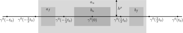
Figure 1. The trajectory $\gamma^{0}$ and the supports of the symbols $a_{u},b_{u},a_{f},b_{f}$.

3.1. Model case

We start the proof of Lemma 3.1 by considering the model case

$$M=\mathbb{R}^{n},\quad P_{h}^{\mathbf{m}}:=hD_{x_{1}},\quad p^{\mathbf{m}}(x,\xi)=\xi_{1},\quad\gamma^{\mathbf{m}}(t)=(t,0,E,0).$$ (3.7)

Here we write elements of $\mathbb{R}^{n}$ as $(x_{1},x^{\prime})$, with $x^{\prime}\in\mathbb{R}^{n-1}$, and elements of $T^{*}\mathbb{R}^{n}$ as $(x_{1},x^{\prime},\xi_{1},\xi^{\prime})$.

Let $t_{0}>0$, choose a function

$$\psi^{\mathbf{m}}\in C_{0}^{\infty}(\mathbb{R}),\quad\operatorname{supp}\psi^{\mathbf{m}}\subset\Big{(}{t_{0}\over 3},{2t_{0}\over 3}\Big{)},\quad\int_{\mathbb{R}}\psi^{\mathbf{m}}(x)\,dx=1,$$

and define

$$\varphi^{\mathbf{m}}\in C_{0}^{\infty}(\mathbb{R}),\quad d_{x}\varphi^{\mathbf{m}}(x)=\psi^{\mathbf{m}}(x+t_{0})-\psi^{\mathbf{m}}(x).$$

Note that

$$\operatorname{supp}\varphi^{\mathbf{m}}\subset\Big{(}-{2t_{0}\over 3},{2t_{0}\over 3}\Big{)},\quad\varphi^{\mathbf{m}}=1\quad\text{near }\Big{[}-{t_{0}\over 3},{t_{0}\over 3}\Big{]}.$$

Define the following $h$-dependent families of functions on $\mathbb{R}^{n}$:

$$u^{\mathbf{m}}(x;h) :=h^{-{n-1\over 4}}\varphi^{\mathbf{m}}(x_{1})e^{i\omega^{2}x_{1}\over h}e^{-{|x^{\prime}|^{2}\over 2h}},$$ (3.8)

$$f^{\mathbf{m}}(x;h) :=ih^{-{n-1\over 4}}\psi^{\mathbf{m}}(x_{1}+t_{0})e^{i\omega^{2}x_{1}\over h}e^{-{|x^{\prime}|^{2}\over 2h}}.$$

It is easy to see that

$$\|u^{\mathbf{m}}(h)\|_{L^{2}},\ \|f^{\mathbf{m}}(h)\|_{L^{2}}\leq C.$$

Moreover, the following analog of (3.2) holds:

$$(P_{h}^{\mathbf{m}}-\omega^{2})u^{\mathbf{m}}(x;h)=h\big{(}e^{it_{0}\omega^{2}/h}f^{\mathbf{m}}(x_{1}-t_{0},x^{\prime};h)-f^{\mathbf{m}}(x;h)\big{)}.$$ (3.9)

We next claim that there exist $a_{u}^{\mathbf{m}},b_{u}^{\mathbf{m}},a_{f}^{\mathbf{m}}\in S^{\operatorname{comp}}_{\rho}(T^{*}\mathbb{R}^{n})$ such that, with $\operatorname{Op}_{h}^{0}$ defined in (2.1) and $\gamma^{\mathbf{m}}_{h^{\rho}}$ defined similarly to (3.1),

$$u^{\mathbf{m}}=\operatorname{Op}_{h}^{0}(a_{u}^{\mathbf{m}})u^{\mathbf{m}}+\mathcal{O}(h^{\infty})_{L^{2}}, \quad\operatorname{supp}a_{u}^{\mathbf{m}}\subset\gamma^{\mathbf{m}}_{h^{\rho}}\big{(}[-2t_{0}/3,2t_{0}/3]\big{)};$$ (3.10)

$$\|\operatorname{Op}^{0}_{h}(b_{u}^{\mathbf{m}})u^{\mathbf{m}}\|_{L^{2}}\geq C^{-1}, \quad\operatorname{supp}b_{u}^{\mathbf{m}}\subset\gamma^{\mathbf{m}}_{h^{\rho}}\big{(}[-t_{0}/4,t_{0}/4]\big{)};$$ (3.11)

$$f^{\mathbf{m}}=\operatorname{Op}^{0}_{h}(a^{\mathbf{m}}_{f})f^{\mathbf{m}}+\mathcal{O}(h^{\infty})_{L^{2}}, \quad\operatorname{supp}a^{\mathbf{m}}_{f}\subset\gamma^{\mathbf{m}}_{h^{\rho}}\big{(}[-2t_{0}/3,-t_{0}/3]\big{)}.$$ (3.12)

Indeed, take $\chi^{\mathbf{m}}\in C_{0}^{\infty}(\mathbb{R})$ such that $\operatorname{supp}\chi^{\mathbf{m}}\subset(-2/3,2/3)$ and $\chi^{\mathbf{m}}=1$ near $t_{0}^{-1}\operatorname{supp}\varphi^{\mathbf{m}}$. Put

$$a^{\mathbf{m}}_{u}(x_{1},x^{\prime},\xi_{1},\xi^{\prime};h):=\chi^{\mathbf{m}}\Big{(}{x_{1}\over t_{0}}\Big{)}\chi^{\mathbf{m}}\Big{(}{\xi_{1}-E\over h^{\rho}}\Big{)}\chi^{\mathbf{m}}\Big{(}{|x^{\prime}|\over h^{\rho}}\Big{)}\chi^{\mathbf{m}}\Big{(}{|\xi^{\prime}|\over h^{\rho}}\Big{)}.$$

It is clear that $a_{u}^{\mathbf{m}}\in S^{\operatorname{comp}}_{\rho}(T^{*}\mathbb{R}^{n})$ and $\operatorname{supp}a_{u}^{\mathbf{m}}\subset\gamma^{\mathbf{m}}_{h^{\rho}}([-2t_{0}/3,2t_{0}/3])$. Next,

$$\operatorname{Op}_{h}^{0}(a^{\mathbf{m}}_{u})=\chi^{\mathbf{m}}\Big{(}{x_{1}\over t_{0}}\Big{)}\chi^{\mathbf{m}}\Big{(}{hD_{x_{1}}-E\over h^{\rho}}\Big{)}\chi^{\mathbf{m}}\Big{(}{|x^{\prime}|\over h^{\rho}}\Big{)}\chi^{\mathbf{m}}\Big{(}{|hD_{x^{\prime}}|\over h^{\rho}}\Big{)}.$$

To check (3.10), it remains to show that each of the functions

$$\chi^{\mathbf{m}}\Big{(}{x_{1}\over t_{0}}\Big{)}u^{\mathbf{m}},\quad\chi^{\mathbf{m}}\Big{(}{hD_{x_{1}}-E\over h^{\rho}}\Big{)}u^{\mathbf{m}},\quad\chi^{\mathbf{m}}\Big{(}{|x^{\prime}|\over h^{\rho}}\Big{)}u^{\mathbf{m}},\quad\chi^{\mathbf{m}}\Big{(}{|hD_{x^{\prime}}|\over h^{\rho}}\Big{)}u^{\mathbf{m}}$$

is equal to $u^{\mathbf{m}}+\mathcal{O}(h^{\infty})_{L^{2}}$. The first of these is trivial as $\varphi^{\mathbf{m}}(x_{1})(1-\chi^{\mathbf{m}}(x_{1}/t_{0}))=0$. The third one follows since $e^{-{|x^{\prime}|^{2}\over 2h}}(1-\chi^{\mathbf{m}}(|x^{\prime}|/h^{\rho}))=\mathcal{O}(h^{\infty})_{L^{2}(\mathbb{R}^{n-1})}$ as long as $\rho<1/2$. The second and fourth operators are Fourier multipliers; to handle them, it suffices to calculate the semiclassical Fourier transform of $u^{\mathbf{m}}$:

$$\mathcal{F}_{h}u^{\mathbf{m}}(\xi;h):=(2\pi h)^{-n/2}\int_{\mathbb{R}^{n}}e^{-{i\langle x,\xi\rangle\over h}}u^{\mathbf{m}}(x;h)\,dx=(2\pi h)^{-1/2}h^{-{n-1\over 4}}\widehat{\varphi^{\mathbf{m}}}\Big{(}{\xi_{1}-\omega^{2}\over h}\Big{)}e^{-{|\xi^{\prime}|^{2}\over 2h}}$$

where $\widehat{\varphi^{\mathbf{m}}}$ is the nonsemiclassical Fourier transform of $\varphi^{\mathbf{m}}$, which is an $h$-independent Schwartz function. Using the bounds

$$\bigg{(}1-\chi^{\mathbf{m}}\Big{(}{\xi_{1}-E\over h^{\rho}}\Big{)}\bigg{)}\widehat{\varphi^{\mathbf{m}}}\Big{(}{\xi_{1}-\omega^{2}\over h}\Big{)} =\mathcal{O}(h^{\infty})_{L^{2}(\mathbb{R})},$$

$$\bigg{(}1-\chi^{\mathbf{m}}\Big{(}{|\xi^{\prime}|\over h^{\rho}}\Big{)}\bigg{)}e^{-{|\xi^{\prime}|^{2}\over 2h}} =\mathcal{O}(h^{\infty})_{L^{2}(\mathbb{R}^{n-1})}$$

and the fact that $\omega^{2}=E+\mathcal{O}(h)$ (following from (1.2)), we finish the proof of (3.10).

We next put

$$b_{u}^{\mathbf{m}}(x_{1},x^{\prime},\xi_{1},\xi^{\prime};h):=\chi^{\mathbf{m}}\Big{(}{4x_{1}\over t_{0}}\Big{)}\chi^{\mathbf{m}}\Big{(}{\xi_{1}-E\over h^{\rho}}\Big{)}\chi^{\mathbf{m}}\Big{(}{|x^{\prime}|\over h^{\rho}}\Big{)}\chi^{\mathbf{m}}\Big{(}{|\xi^{\prime}|\over h^{\rho}}\Big{)}.$$

Then (3.11) follows from the following fact, which is proved similarly to (3.10):

$$\operatorname{Op}_{h}^{0}(b^{\mathbf{m}}_{u})u^{\mathbf{m}}(x;h)=h^{-{n-1\over 4}}\chi^{\mathbf{m}}\Big{(}{4x_{1}\over t_{0}}\Big{)}e^{i\omega^{2}x_{1}\over h}e^{-{|x^{\prime}|^{2}\over 2h}}+\mathcal{O}(h^{\infty})_{L^{2}}.$$

The bound (3.12) is proved similarly to (3.10), taking

$$a_{f}^{\mathbf{m}}(x_{1},x^{\prime},\xi_{1},\xi^{\prime};h):=\chi_{1}^{\mathbf{m}}(x_{1}+t_{0})\chi^{\mathbf{m}}\Big{(}{\xi_{1}-E\over h^{\rho}}\Big{)}\chi^{\mathbf{m}}\Big{(}{|x^{\prime}|\over h^{\rho}}\Big{)}\chi^{\mathbf{m}}\Big{(}{|\xi^{\prime}|\over h^{\rho}}\Big{)}$$

where $\chi_{1}^{\mathbf{m}}\in C_{0}^{\infty}(\mathbb{R})$ is supported in $(t_{0}/3,2t_{0}/3)$ and equal to 1 near $\operatorname{supp}\psi^{\mathbf{m}}$.

3.2. General case

We now prove Lemma 3.1. For that, we reduce to the model case of §3.1 using conjugation by Fourier integral operators.

By (1.4), we have $dp(\tilde{x}_{0},\tilde{\xi}_{0})\neq 0$. Therefore, by Darboux Theorem [HöIII, Theorem 21.1.6], there exists a symplectomorphism

$$\varkappa:U_{\varkappa}\to V_{\varkappa},\quad(\tilde{x}_{0},\tilde{\xi}_{0})\in U_{\varkappa}\subset T^{*}M,\quad V_{\varkappa}\subset T^{*}\mathbb{R}^{n},$$

such that

$$\varkappa(\tilde{x}_{0},\tilde{\xi}_{0})=(0,0,E,0),\quad p=\xi_{1}\circ\varkappa\quad\text{on }U_{\varkappa}.$$

Take $t_{0}>0$ such that $\gamma^{0}([-t_{0},t_{0}])\subset U_{\varkappa}$. Then for $|t|\leq t_{0}$, we have $\varkappa(\gamma^{0}(t))=\gamma^{\mathbf{m}}(t)$, with $\gamma^{\mathbf{m}}$ defined in (3.7).

For $t_{0}$ small enough, there exist Fourier integral operators

$$B\in I^{\operatorname{comp}}(\varkappa),\quad B^{\prime}\in I^{\operatorname{comp}}(\varkappa^{-1})$$

such that

$$B^{\prime}B=1+\mathcal{O}(h^{\infty}) \quad\text{microlocally near }\gamma^{0}([-t_{0},t_{0}]),$$ (3.13)

$$BB^{\prime}=1+\mathcal{O}(h^{\infty}) \quad\text{microlocally near }\gamma^{\mathbf{m}}([-t_{0},t_{0}]),$$ (3.14)

$$P_{h}B^{\prime}=B^{\prime}(hD_{x_{1}})+\mathcal{O}(h^{\infty}) \quad\text{microlocally near }\gamma^{0}([-t_{0},t_{0}])\times\gamma^{\mathbf{m}}([-t_{0},t_{0}]).$$ (3.15)

See for instance [Zw, Theorem 12.3] for the proof.

We now put

$$u_{0}(h):=B^{\prime}u^{\mathbf{m}}(h),\quad f_{0}(h):=B^{\prime}f^{\mathbf{m}}(h),$$

with $u^{\mathbf{m}},f^{\mathbf{m}}$ defined in (3.8).

Since $\|B^{\prime}\|_{L^{2}(\mathbb{R}^{n})\to L^{2}(M)}=\mathcal{O}(1)$, we have $\|u_{0}\|_{L^{2}},\|f_{0}\|_{L^{2}}\leq C$. Note that (3.6) holds for $u^{\mathbf{m}},f^{\mathbf{m}},\gamma^{\mathbf{m}}$ by (3.10) and (3.12); since $\operatorname{WF}_{h}(B^{\prime})$ lies inside the graph of $\varkappa^{-1}$, we see that (3.6) holds for $u_{0},f_{0},\gamma^{0}$. In particular, it will be enough to argue microlocally near $\gamma^{0}([-t_{0},t_{0}])$.

The identity (3.2) follows from (3.9), (3.13), (3.15), and the following statement:

$$e^{-itP_{h}/h}f_{0}=B^{\prime}f^{\mathbf{m}}_{t}+\mathcal{O}(h^{\infty})_{L^{2}},\ 0\leq t\leq t_{0};\quad f^{\mathbf{m}}_{t}(x_{1},x^{\prime};h):=f^{\mathbf{m}}(x_{1}-t,x^{\prime};h).$$ (3.16)

Since (3.16) is true for $t=0$, it suffices to show that

$$\partial_{t}(e^{itP_{h}/h}B^{\prime}f^{\mathbf{m}}_{t})=\mathcal{O}(h^{\infty})_{L^{2}},\quad 0\leq t\leq t_{0}.$$

This in turn can be rewritten as

$${i\over h}e^{itP_{h}/h}(P_{h}B^{\prime}-B^{\prime}hD_{x_{1}})f^{\mathbf{m}}_{t}=\mathcal{O}(h^{\infty})_{L^{2}},\quad 0\leq t\leq t_{0},$$

which follows from (3.15) and the fact that $\operatorname{WF}_{h}(f^{\mathbf{m}}_{t})\subset\gamma^{\mathbf{m}}([t-2t_{0}/3,t-t_{0}/3])$.

The estimates (3.3)–(3.5) follow from (3.10)–(3.12), if we choose $a_{u},b_{u},a_{f}$ such that

$$B^{\prime}\operatorname{Op}_{h}(a^{\mathbf{m}}_{u})=\operatorname{Op}_{h}(a_{u})B^{\prime}+\mathcal{O}(h^{\infty})_{L^{2}\to L^{2}},$$

and similarly for $b_{u},a_{f}$. To do that, it suffices to multiply (2.4) on the right by $B^{\prime}$ and use (3.14). If we carry out the arguments of §3.1 with $\rho$ replaced by some $\rho^{\prime}\in(\rho,1/2)$, then we have for small $h$

$$\operatorname{supp}a_{u}\ \subset\ \varkappa^{-1}\big{(}\gamma^{\mathbf{m}}_{h^{\rho^{\prime}}}\big{(}[-2t_{0}/3,2t_{0}/3]\big{)}\big{)}\ \subset\ \gamma^{0}_{h^{\rho}}\big{(}[-2t_{0}/3,2t_{0}/3]\big{)}$$

and similarly for $a_{f}$; this finishes the proofs of (3.3), (3.5).

For (3.4), we additionally use that

$$\|\operatorname{Op}_{h}^{0}(b^{\mathbf{m}}_{u})u^{\mathbf{m}}\|_{L^{2}}\leq C\|BB^{\prime}\operatorname{Op}_{h}^{0}(b^{\mathbf{m}}_{u})u^{\mathbf{m}}\|_{L^{2}}+\mathcal{O}(h^{\infty})\leq C\|\operatorname{Op}_{h}(b_{u})u_{0}\|_{L^{2}}+\mathcal{O}(h^{\infty}).$$

This finishes the proof of Lemma 3.1.

4. Long Gaussian beam

We now construct a Gaussian beam localized on a $\sim\log(1/h)$ long trajectory of the flow $e^{tH_{p}}$. Recall the trajectory $\gamma$ defined in (1.5) and the associated constant $\lambda_{\max}\geq 0$ defined in (1.6).

Lemma 4.1.

Let $\beta>0$ satisfy (1.7). If $t_{0}>0$ is small enough, then there exist $h$-dependent functions $u=u(h),f_{\pm}=f_{\pm}(h)\in C_{0}^{\infty}(M)$ such that:

1. We have $\|u\|_{L^{2}}\leq C$, $\|f_{+}\|_{L^{2}}\leq C$, and $\|f_{-}\|_{L^{2}}\leq Ch^{2\sqrt{E}\beta\nu}$ for some $h$-independent constant $C$, and $u,f_{\pm}$ are supported inside some $h$-independent compact subset of $M$.

2. $(P_{h}-\omega^{2})u=h(f_{+}-f_{-})+\mathcal{O}(h^{\infty})_{L^{2}}$.

3. $\operatorname{WF}_{h}(f_{+})\subset\gamma([t_{0}/3,2t_{0}/3])$.

4. There exists $b\in S^{\operatorname{comp}}_{\rho}(T^{*}M)$ with $\operatorname{supp}b$ contained in an $o(1)$ neighborhood of $\gamma([-t_{0}/4,t_{0}/4])$ as $h\to 0$ and such that $\|\operatorname{Op}_{h}(b)u\|_{L^{2}}\geq C^{-1}$.

We start the proof of Lemma 4.1 by taking $t_{0}$ small enough so that Lemma 3.1 applies to

$$(\tilde{x}_{0},\tilde{\xi}_{0}):=\gamma\Big{(}-{\beta\over 2}\log(1/h)\Big{)},\quad\gamma^{0}(t)=\gamma\Big{(}t-{\beta\over 2}\log(1/h)\Big{)}.$$ (4.1)

We also change $t_{0}$ slighly in an $h$-dependent way so that

$$N_{0}:={\beta\over 2t_{0}}\log(1/h)$$

is an integer. Using (1.7), take $\lambda,\rho$ such that

$$\lambda>\lambda_{\max},\quad\rho\in[0,1/2),\quad\lambda\beta<2\rho.$$ (4.2)

Let $u_{0},f_{0}$ be the functions constructed in Lemma 3.1. Let $\chi\in C_{0}^{\infty}(M;[0,1])$ satisfy

$$\chi=1\quad\text{near the closure of }\gamma\big{(}(-\infty,2t_{0}]\big{)}.$$ (4.3)

For $j\in\mathbb{Z}$, define $u_{j}=u_{j}(h),f_{j}=f_{j}(h)\in C_{0}^{\infty}(M)$ inductively starting from $u_{0},f_{0}$:

$$u_{j+1}:=\chi e^{-it_{0}(P_{h}-\omega^{2})/h}u_{j}, \quad f_{j+1}:=\chi e^{-it_{0}(P_{h}-\omega^{2})/h}f_{j}, \quad j\geq 0;$$

$$u_{j-1}:=\chi e^{it_{0}(P_{h}-\omega^{2})/h}u_{j}, \quad f_{j-1}:=\chi e^{it_{0}(P_{h}-\omega^{2})/h}f_{j}, \quad j\leq 0.$$

We now define

$$u:=h^{\sqrt{E}\beta\nu}\sum_{j=-N_{0}}^{N_{0}}u_{j},\quad f_{+}:=h^{\sqrt{E}\beta\nu}f_{N_{0}+1},\quad f_{-}:=h^{\sqrt{E}\beta\nu}f_{-N_{0}}.$$ (4.4)

Note that by (1.2),

$$|e^{it_{0}N_{0}\omega^{2}/h}|=h^{-\sqrt{E}\beta\nu}.$$

Therefore, part 1 of Lemma 4.1 is satisfied.

The remaining parts of Lemma 4.1 use the following localization statement for $u_{j},f_{j}$, proved in §4.1 (see Figure 2):

Lemma 4.2.

For each $j\in[-N_{0},N_{0}+1]$, there exist $a_{u}^{(j)},b_{u}^{(j)},a_{f}^{(j)}\in S^{\operatorname{comp}}_{\rho}(T^{*}M)$, bounded uniformly in $j$, such that, with remainders uniform in $j$,

$$u_{j} =\operatorname{Op}_{h}(a_{u}^{(j)})u_{j}+\mathcal{O}(h^{\infty})_{L^{2}},$$ (4.5)

$$\operatorname{supp}a_{u}^{(j)} \subset\gamma_{Ce^{|j|\lambda t_{0}}h^{\rho}}\Big{(}\Big{[}\Big{(}j-N_{0}-{2\over 3}\Big{)}t_{0},\Big{(}j-N_{0}+{2\over 3}\Big{)}t_{0}\Big{]}\Big{)};$$ (4.6)

$$\|\operatorname{Op}_{h}(b_{u}^{(j)})u_{j}\|_{L^{2}} \geq C^{-1}e^{2\sqrt{E}\nu t_{0}j},$$ (4.7)

$$\operatorname{supp}b_{u}^{(j)} \subset\gamma_{Ce^{|j|\lambda t_{0}}h^{\rho}}\Big{(}\Big{[}\Big{(}j-N_{0}-{1\over 4}\Big{)}t_{0},\Big{(}j-N_{0}+{1\over 4}\Big{)}t_{0}\Big{]}\Big{)};$$ (4.8)

$$f_{j} =\operatorname{Op}_{h}(a_{f}^{(j)})f_{j}+\mathcal{O}(h^{\infty})_{L^{2}},$$ (4.9)

$$\operatorname{supp}a_{f}^{(j)} \subset\gamma_{Ce^{|j|\lambda t_{0}}h^{\rho}}\Big{(}\Big{[}\Big{(}j-N_{0}-{2\over 3}\Big{)}t_{0},\Big{(}j-N_{0}-{1\over 3}\Big{)}t_{0}\Big{]}\Big{)};$$ (4.10)

where $C$ is independent of $h$ and $j$ and $\gamma_{\varepsilon}(U)$ denotes the $\varepsilon$-neighborhood of $\gamma(U)$.

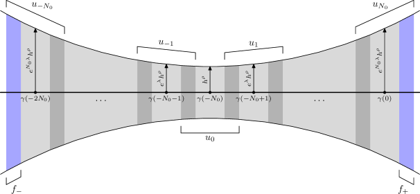
Figure 2. The shaded region represents microlocal concentration of the function $u$ from (4.4), where we put $t_{0}=1$ for simplicity of notation. The darker regions represent the places where the summands $u_{j}$ and $u_{j+1}$ overlap, and the blue regions at the ends correspond to $f_{\pm}$.

We remark that by (4.2),

$$Ce^{N_{0}\lambda t_{0}}h^{\rho}=Ch^{\rho-{\lambda\beta\over 2}}\to 0\quad\text{as }h\to 0,$$

therefore the sets in (4.6), (4.8), and (4.10) are contained in $o(1)$ neighborhoods of the corresponding segments of $\gamma$.

Given Lemma 4.2, we claim that uniformly in $j\in[-N_{0},N_{0}]$,

$$(P_{h}-\omega^{2})u_{j}=h(f_{j+1}-f_{j})+\mathcal{O}(h^{\infty})_{L^{2}}.$$ (4.11)

For $j=0$, (4.11) follows from (3.2) and the following corollary of (2.5), (4.3), and (4.9):

$$(1-\chi)e^{-it_{0}(P_{h}-\omega^{2})/h}f_{0}=\mathcal{O}(h^{\infty})_{L^{2}}.$$ (4.12)

Now, assume that (4.11) holds for some $j\in[0,N_{0}-1]$. Then

$$(P_{h}-\omega^{2})u_{j+1} =[P_{h},\chi]e^{-it_{0}(P_{h}-\omega^{2})/h}u_{j}+\chi e^{-it_{0}(P_{h}-\omega^{2})/h}(P_{h}-\omega^{2})u_{j}$$

$$=[P_{h},\chi]e^{-it_{0}(P_{h}-\omega^{2})/h}u_{j}+\chi e^{-it_{0}(P_{h}-\omega^{2})/h}h(f_{j+1}-f_{j})+\mathcal{O}(h^{\infty})_{L^{2}}.$$

The first term on the right-hand side is $\mathcal{O}(h^{\infty})_{L^{2}}$ as follows from (2.5), (4.3), and (4.5). The second term is equal to $h(f_{j+2}-f_{j+1})$; therefore, we see that (4.11) holds for $j+1$. Arguing by induction on $j=0,\dots,N_{0}-1$ (since the number of iterations is bounded by a constant times $\log(1/h)$, it is easy to verify that the $\mathcal{O}(h^{\infty})$ remainder is uniform in $j$), we obtain (4.11) for all $j\in[0,N_{0}]$. Arguing similarly, we obtain (4.11) for all $j\in[-N_{0},-1]$ as well; here the case $j=-1$ has to be handled separately using the following corollary of (4.3), (4.9), and (4.12):

$$\chi e^{it_{0}(P_{h}-\omega^{2})/h}f_{1}=f_{0}+\mathcal{O}(h^{\infty})_{L^{2}}.$$

Adding together (4.11) for all $j=-N_{0},\dots,N_{0}$, we obtain part 2 of Lemma 4.1. Part 3 of Lemma 4.1 follows immediately from (4.9).

Finally, for part 4 of Lemma 4.1, we put $b:=b^{(N_{0})}_{u}$. By (4.7), we have $\|\operatorname{Op}_{h}(b)u\|_{L^{2}}\geq C^{-1}$ as long as

$$\operatorname{Op}_{h}(b)u_{j}=\mathcal{O}(h^{\infty})_{L^{2}}\quad\text{uniformly in }j\in[-N_{0},N_{0}-1].$$

This follows from (4.5) and the following statement:

$$\operatorname{supp}b\cap\operatorname{supp}a_{u}^{(j)}=\emptyset\quad\text{for $h$ small enough and all }j\in[-N_{0},N_{0}-1].$$ (4.13)

The identity (4.13) follows from (4.6), (4.8) and the fact that there exists $\varepsilon>0$ such that

$$d(\gamma(t_{1}),\gamma(t_{2}))>\varepsilon\quad\text{for all }t_{1}\in\Big{[}-{t_{0}\over 4},{t_{0}\over 4}\Big{]},\ t_{2}\in\Big{(}-\infty,-{t_{0}\over 3}\Big{]}.$$ (4.14)

To show (4.14), we note that $\gamma(t)$ is not trapped in the forward direction, thus it is not a closed trajectory; it follows that $\gamma(t_{1})\neq\gamma(t_{2})$ for $t_{2}\leq-t_{0}/3<-t_{0}/4\leq t_{1}$. It remains to show that for each $t_{j}\to-\infty$, $\gamma(t_{j})$ cannot converge to a point in $\gamma([-t_{0}/4,t_{0}/4])$; this follows from the fact that $\gamma([-t_{0}/4,t_{0}/4])$ does not intersect the trapped set, but the backwards trapped trajectory $\gamma(t)$ converges to the trapped set as $t\to-\infty$ – see for instance [Dy15, Lemma 4.1]. This finishes the proof of Lemma 4.1.

4.1. Localization of the long beam

We now prove Lemma 4.2. Fix $\lambda_{1},\lambda_{2}$ such that

$$\lambda_{\max}<\lambda_{1}<\lambda_{2}<\lambda.$$

We start by constructing metrics on $T^{*}M$ which are adapted to the flow $e^{tH_{p}}$ on the trajectory $\gamma$:

Lemma 4.3.

There exist smooth $h$-independent Riemannian metrics $\tilde{g}_{\pm}$ on $T^{*}M$ such that

$$|de^{\pm t_{0}H_{p}}(\gamma(t))v|_{\tilde{g}_{\pm}}\leq e^{\lambda_{1}t_{0}}|v|_{\tilde{g}_{\pm}},\quad t\in(-\infty,0],\ v\in T_{\gamma(t)}(T^{*}M).$$ (4.15)

Proof.

Fix a Riemannian metric $\tilde{g}_{0}$ on $T^{*}M$. By (1.6), for $T>0$ large enough

$$|de^{TH_{p}}(\gamma(t))v|_{\tilde{g}_{0}}\leq e^{\lambda_{1}T}|v|_{\tilde{g}_{0}}, \quad t\in(-\infty,t_{0}-T],\quad v\in T_{\gamma(t)}(T^{*}M);$$ (4.16)

$$|de^{-TH_{p}}(\gamma(t))v|_{\tilde{g}_{0}}\leq e^{\lambda_{1}T}|v|_{\tilde{g}_{0}}, \quad t\in(-\infty,t_{0}],\quad v\in T_{\gamma(t)}(T^{*}M).$$ (4.17)

Define the metrics $\tilde{g}_{\pm}$ as follows: for $(x,\xi)\in T^{*}M$ and $u,v\in T_{(x,\xi)}(T^{*}M)$, put

$$\langle u,v\rangle_{\tilde{g}_{\pm}(x,\xi)}:=\int_{0}^{T}e^{\pm 2\lambda_{1}s}\langle de^{-sH_{p}}(x,\xi)u,de^{-sH_{p}}(x,\xi)v\rangle_{\tilde{g}_{0}(e^{-sH_{p}}(x,\xi))}\,ds.$$

Take $t\leq 0$ and $v\in T_{\gamma(t)}(T^{*}M)$. Then

$$|de^{t_{0}H_{p}}(\gamma(t))v|^{2}_{\tilde{g}_{+}}=\int_{0}^{T}e^{2\lambda_{1}s}|de^{(t_{0}-s)H_{p}}(\gamma(t))v|^{2}_{\tilde{g}_{0}}\,ds,$$

therefore

$$\begin{gathered}|de^{t_{0}H_{p}}(\gamma(t))v|^{2}_{\tilde{g}_{+}}-e^{2\lambda_{1}t_{0}}|v|^{2}_{\tilde{g}_{+}}\\ =\int_{0}^{T}e^{2\lambda_{1}s}|de^{(t_{0}-s)H_{p}}(\gamma(t))v|^{2}_{\tilde{g}_{0}}\,ds-\int_{t_{0}}^{T+t_{0}}e^{2\lambda_{1}s}|de^{(t_{0}-s)H_{p}}(\gamma(t))v|^{2}_{\tilde{g}_{0}}\,ds\\ =\int_{0}^{t_{0}}e^{2\lambda_{1}s}\Big{(}|de^{(t_{0}-s)H_{p}}(\gamma(t))v|_{\tilde{g}_{0}}^{2}-e^{2\lambda_{1}T}|de^{(t_{0}-s-T)H_{p}}(\gamma(t))v|_{\tilde{g}_{0}}^{2}\Big{)}\,ds\leq 0,\end{gathered}$$

where the last inequality follows from (4.16) with $t,v$ replaced by $t_{0}-s-T+t$, $de^{(t_{0}-s-T)H_{p}}(\gamma(t))v$. This proves the ‘$+$’ part of (4.15).

We similarly have

$$\begin{gathered}|de^{-t_{0}H_{p}}(\gamma(t))v|^{2}_{\tilde{g}_{-}}-e^{2\lambda_{1}t_{0}}|v|^{2}_{\tilde{g}_{-}}\\ =\int_{-t_{0}}^{0}e^{-2\lambda_{1}s}\Big{(}e^{-2\lambda_{1}T}|de^{-(t_{0}+T+s)H_{p}}(\gamma(t))v|^{2}_{\tilde{g}_{0}}-|de^{-(t_{0}+s)H_{p}}(\gamma(t))v|^{2}_{\tilde{g}_{0}}\Big{)}\,ds\leq 0,\end{gathered}$$

where the last inequality follows from (4.17) with $t,v$ replaced by $t-t_{0}-s$, $de^{-(t_{0}+s)H_{p}}(\gamma(t))v$. This proves the ‘$-$’ part of (4.15). ∎

We next construct tubular neighborhoods of segments of $\gamma$. Fix small $\delta>0$ to be chosen later. For each $t\leq t_{0}$, define the manifold

$$V^{\pm}_{t}=\{(s,v)\mid s\in(-t_{0},t_{0}),\ v\in T_{\gamma(t+s)}(T^{*}M),\ v\perp_{\tilde{g}_{\pm}}H_{p}(\gamma(t+s)),\ |v|_{\tilde{g}_{\pm}}<\delta\}.$$

Define the maps

$$\Phi^{\pm}_{t}:V^{\pm}_{t}\to T^{*}M,\quad\Phi^{\pm}_{t}(s,v)=\exp^{\tilde{g}_{\pm}}_{\gamma(t+s)}(v),$$

where $\exp^{\tilde{g}_{\pm}}_{\bullet}(\bullet)$ denotes the geodesic exponential map of the metric $\tilde{g}_{\pm}$. By (1.4), for $t_{0}$ and $\delta$ small enough the maps $\Phi^{\pm}_{t}$ are diffeomorphisms onto their images uniformly in $t\leq t_{0}$. Note that $\Phi^{\pm}_{t}(s,0)=\gamma(t+s)$.

Lemma 4.4.

For $\varepsilon>0$ small enough and all

$$t\leq 0,\quad(s,v)\in V^{\pm}_{t},\quad|s|\leq{3t_{0}\over 4},\quad|v|_{\tilde{g}_{\pm}}\leq\varepsilon,$$

there exist unique $(S_{\pm},v_{\pm})\in V^{\pm}_{t\pm t_{0}}$ such that for some global constant $C$,

$$e^{\pm t_{0}H_{p}}(\Phi^{\pm}_{t}(s,v))=\Phi^{\pm}_{t\pm t_{0}}(S_{\pm},v_{\pm}),\quad|S_{\pm}-s|\leq C|v|_{\tilde{g}_{\pm}},\quad|v_{\pm}|_{\tilde{g}_{\pm}}\leq e^{\lambda_{2}t_{0}}|v|_{\tilde{g}_{\pm}}.$$ (4.18)

Proof.

For $v=0$, we have

$$S_{\pm}(s,0)=s,\quad v_{\pm}(s,0)=0.$$

Since all derivatives of $\Phi^{\pm}_{t}$ and its inverse are bounded uniformly in $t$, we deduce the existence and uniqueness of $S_{\pm}(s,v),v_{\pm}(s,v)$ for $|s|\leq{3\over 4}t_{0}$ and $|v|$ small enough.

Next, note that

$$\partial_{s}S_{\pm}(s,0)=1,\quad\partial_{s}v_{\pm}(s,0)=0.$$

Also, if $w\in T_{\gamma(t+s)}(T^{*}M)$ and $w\perp_{\tilde{g}_{\pm}}H_{p}(\gamma(t+s))$, then

$$\partial_{v}S_{\pm}(s,0)w=\zeta_{\pm},\quad\partial_{v}v_{\pm}(s,0)w=w_{\pm},$$

where $\zeta_{\pm}\in\mathbb{R}$, $w_{\pm}\in T_{\gamma(t\pm t_{0}+s)}(T^{*}M)$, $w_{\pm}\perp_{\tilde{g}_{\pm}}H_{p}(\gamma(t\pm t_{0}+s))$, are determined uniquely from the equation

$$de^{\pm t_{0}H_{p}}(\gamma(t+s))w=\zeta_{\pm}H_{p}(\gamma(t\pm t_{0}+s))+w_{\pm}.$$

By (4.15), we have

$$|\zeta_{\pm}|\leq C|w|_{\tilde{g}_{\pm}},\quad|w_{\pm}|_{\tilde{g}_{\pm}}\leq e^{\lambda_{1}t_{0}}|w|_{\tilde{g}_{\pm}}.$$

Since all derivatives of $\Phi^{\pm}_{t}$ and its inverse are bounded uniformly in $t$, it follows that for $\varepsilon>0$ small enough and $|v|_{\tilde{g}_{\pm}}\leq\varepsilon$, the inequalities in (4.18) hold. ∎

We now construct the functions $a^{(j)}_{u},b^{(j)}_{u},a^{(j)}_{f}$ from Lemma 4.2. Let $C_{0}>0$ be a large fixed constant. For $t_{1}<t_{2}$ and $j\in[-N_{0},N_{0}]$, define the functions

$$\psi^{(j)}_{[t_{1},t_{2}]}(s)=\psi_{0}\Big{(}{t-t_{1}\over C_{0}^{2}e^{|j|\lambda t_{0}}h^{\rho}}\Big{)}\psi_{0}\Big{(}{t_{2}-t\over C_{0}^{2}e^{|j|\lambda t_{0}}h^{\rho}}\Big{)},\quad s\in\mathbb{R},$$

where $\psi_{0}\in C^{\infty}(\mathbb{R};[0,1])$ satisfies $\psi_{0}=0$ near $(-\infty,-1]$ and $\psi_{0}=1$ near $[-e^{-\lambda_{2}t},\infty)$. Note that for fixed $t_{1},t_{2}$, the function $\psi^{(j)}_{[t_{1},t_{2}]}$ is in $S^{\operatorname{comp}}_{\rho}$ uniformly in $j$ and

$$\operatorname{supp}\psi^{(j)}_{[t_{1},t_{2}]} \subset\big{(}t_{1}-C_{0}^{2}e^{|j|\lambda t_{0}}h^{\rho},t_{2}+C_{0}^{2}e^{|j|\lambda t_{0}}h^{\rho}\big{)},$$ (4.19)

$$\psi^{(j)}_{[t_{1},t_{2}]}=1\quad \text{near }\big{[}t_{1}-C_{0}^{2}e^{(|j|\lambda-\lambda_{2})t_{0}}h^{\rho},t_{2}+C_{0}^{2}e^{(|j|\lambda-\lambda_{2})t_{0}}h^{\rho}\big{]}.$$ (4.20)

Next, take $\chi_{0}\in C_{0}^{\infty}\big{(}(-e^{\lambda t_{0}},e^{\lambda t_{0}});[0,1]\big{)}$ such that $\chi_{0}=1$ near $[-e^{\lambda_{2}t_{0}},e^{\lambda_{2}t_{0}}]$, and put

$$\chi^{(j)}(r)=\chi_{0}\Big{(}{r\over C_{0}e^{|j|\lambda t_{0}}h^{\rho}}\Big{)},\quad r\in\mathbb{R},\quad j\in[-N_{0},N_{0}];$$

note that $\chi^{(j)}\in S^{\operatorname{comp}}_{\rho}$ uniformly in $j$ and

$$\operatorname{supp}\chi^{(j)} \subset\{|r|<C_{0}e^{(|j|+1)\lambda t_{0}}h^{\rho}\},$$ (4.21)

$$\chi^{(j)}=1\quad \text{near }\{|r|\leq C_{0}e^{(|j|\lambda+\lambda_{2})t_{0}}h^{\rho}\}.$$ (4.22)

We define $a^{(j)}_{u},b^{(j)}_{u},a^{(j)}_{f}$ for $j\in[0,N_{0}+1]$ as follows:

$$a^{(j)}_{u},b^{(j)}_{u},a^{(j)}_{f} \in C_{0}^{\infty}(\Phi^{+}_{(j-N_{0})t_{0}}(V^{+}_{(j-N_{0})t_{0}})),$$

$$a^{(j)}_{u}(\Phi^{+}_{(j-N_{0})t_{0}}(s,v)) =\psi^{(j)}_{[-2t_{0}/3,2t_{0}/3]}(s)\cdot\chi^{(j)}\big{(}|v|_{\tilde{g}_{+}}\big{)},$$

$$b^{(j)}_{u}(\Phi^{+}_{(j-N_{0})t_{0}}(s,v)) =\psi^{(j)}_{[-t_{0}/4,t_{0}/4]}(s)\cdot\chi^{(j)}\big{(}|v|_{\tilde{g}_{+}}\big{)},$$

$$a^{(j)}_{f}(\Phi^{+}_{(j-N_{0})t_{0}}(s,v)) =\psi^{(j)}_{[-2t_{0}/3,-t_{0}/3]}(s)\cdot\chi^{(j)}\big{(}|v|_{\tilde{g}_{+}}\big{)}.$$

The resulting symbols are in $S^{\operatorname{comp}}_{\rho}(T^{*}M;[0,1])$ uniformly in $j$; moreover, by (4.19) and (4.21) the support conditions (4.6), (4.8), and (4.10) are satisfied. Using (4.18) and (4.19)–(4.22) we see that for $C_{0}$ large enough,

$$e^{t_{0}H_{p}}(\operatorname{supp}a^{(j)}_{u})\cap\operatorname{supp}(1-a^{(j+1)}_{u})=\emptyset,\quad j\in[0,N_{0}],$$ (4.23)

and similarly for $b^{(j)}_{u},a^{(j)}_{f}$.

Next, we prove (4.5), (4.7), and (4.9). The case $j=0$ follows directly from (3.3), (3.4), and (3.5), using (2.3) and taking $C_{0}$ large enough so that (recalling (4.1), (4.20), and (4.22)) $\operatorname{supp}a_{u}\cap\operatorname{supp}(1-a^{(0)}_{u})=\emptyset$ and similarly for $b_{u},a_{f}$.

We now argue by induction. Assume that (4.5) holds for some $j\in[0,N_{0}]$. By (2.5), there exists $\tilde{a}^{(j)}_{u}\in S^{\operatorname{comp}}_{\rho}(T^{*}M)$ such that

$$e^{-it_{0}P_{h}/h}\operatorname{Op}_{h}(a^{(j)}_{u})e^{it_{0}P_{h}/h}=\operatorname{Op}_{h}(\tilde{a}^{(j)}_{u})+\mathcal{O}(h^{\infty})_{L^{2}\to L^{2}}.$$

Here the constants in the $\mathcal{O}(h^{\infty})$ remainder are uniform in $j$, since all $S^{\operatorname{comp}}_{\rho}$ seminorms of $a^{(j)}_{u}$ are bounded uniformly in $j$; similar reasoning applies to the $\mathcal{O}(h^{\infty})$ remainders below.

Applying $e^{-it_{0}P_{h}/h}$ to (4.5) for $j$, we obtain

$$e^{-it_{0}P_{h}/h}u_{j}=\operatorname{Op}_{h}(\tilde{a}^{(j)}_{u})e^{-it_{0}P_{h}/h}u_{j}+\mathcal{O}(h^{\infty})_{L^{2}}.$$

We may choose $\tilde{a}^{(j)}_{u}$ so that $\operatorname{supp}\tilde{a}^{(j)}_{u}\subset e^{t_{0}H_{p}}(\operatorname{supp}a^{(j)}_{u})$. Then by (2.3), (4.3), and (4.23) we see that

$$\chi e^{-it_{0}P_{h}/h}u_{j}=\operatorname{Op}_{h}(a^{(j+1)}_{u})\chi e^{-it_{0}P_{h}/h}u_{j}+\mathcal{O}(h^{\infty})_{L^{2}},$$

therefore (4.5) holds for $j+1$. Using induction on $j$, we obtain (4.5) for all $j\in[0,N_{0}+1]$, where it is easy to see that the $\mathcal{O}(h^{\infty})$ remainder is uniform in $j$ since the number of iterations is $\mathcal{O}(\log(1/h))$. A similar argument shows that (4.9) holds for all $j\in[0,N_{0}+1]$.

Next, (4.7) for $j\in[0,N_{0}+1]$ follows by induction on $j$ together with the following estimate:

$$\|\operatorname{Op}_{h}(b^{(j)}_{u})u_{j}\|_{L^{2}}\leq(1+Ch^{1/2-\rho})\|\operatorname{Op}_{h}(b^{(j+1)}_{u})\chi e^{-it_{0}P_{h}/h}u_{j}\|_{L^{2}}+\mathcal{O}(h^{\infty}).$$ (4.24)

To show (4.24), note first that $\chi$ on the right-hand side may be replaced by $1$ by (4.3). By (2.5), there exists $\tilde{b}^{(j)}_{u}\in S^{\operatorname{comp}}_{\rho}(T^{*}M)$ such that

$$e^{-it_{0}P_{h}/h}\operatorname{Op}_{h}(b^{(j)}_{u})e^{it_{0}P_{h}/h}=\operatorname{Op}_{h}(\tilde{b}^{(j)}_{u})+\mathcal{O}(h^{\infty})_{L^{2}\to L^{2}};$$

moreover, we may assume that $\operatorname{supp}\tilde{b}^{(j)}_{u}\subset e^{t_{0}H_{p}}(\operatorname{supp}b^{(j)}_{u})$. Then

$$\|\operatorname{Op}_{h}(b^{(j)}_{u})u_{j}\|_{L^{2}} =\|e^{-it_{0}P_{h}/h}\operatorname{Op}_{h}(b^{(j)}_{u})u_{j}\|_{L^{2}}$$

$$=\|\operatorname{Op}_{h}(\tilde{b}^{(j)}_{u})e^{-it_{0}P_{h}/h}u_{j}\|_{L^{2}}+\mathcal{O}(h^{\infty})$$

$$=\|\operatorname{Op}_{h}(\tilde{b}^{(j)}_{u})\operatorname{Op}_{h}(b^{(j+1)}_{u})e^{-it_{0}P_{h}/h}u_{j}\|_{L^{2}}+\mathcal{O}(h^{\infty})$$

where the last line above follows from (2.3) and the analog of (4.23) for $b^{(j)}_{u}$. To prove (4.24), it remains to use the norm bound

$$\|\operatorname{Op}_{h}(\tilde{b}^{(j)}_{u})\|_{L^{2}\to L^{2}}\leq 1+Ch^{{1\over 2}-\rho},$$ (4.25)

To show (4.25), we first note that $\tilde{b}^{(j)}_{u}=b^{(j)}_{u}\circ e^{-t_{0}H_{p}}+\mathcal{O}(h^{1-2\rho})$ and $|b^{(j)}_{u}|\leq 1$; therefore, the principal symbol of $\operatorname{Op}_{h}(\tilde{b}^{(j)}_{u})$ is bounded above by $1+\mathcal{O}(h^{1-2\rho})$. Since $t_{0}$ is small, $\tilde{b}^{(j)}_{u}$ is supported in some coordinate chart on $M$; thus it suffices to show the bound

$$\|\operatorname{Op}_{h}^{0}(b)\|_{L^{2}\to L^{2}}\leq\sup_{T^{*}M}|b|+\mathcal{O}(h^{{1\over 2}-\rho}),\quad b\in S^{\operatorname{comp}}_{\rho}(T^{*}\mathbb{R}^{n})$$ (4.26)

where $\operatorname{Op}_{h}^{0}$ is defined in (2.1). The bound (4.26) follows from [Zw, Theorem 4.23(ii)].

We have proven (4.5)–(4.10) for $j\in[0,N_{0}+1]$. The case $j\in[-N_{0},0]$ is considered in the same way, using the metric $\tilde{g}_{-}$ instead of $\tilde{g}_{+}$ in the definitions of $a^{(j)}_{u},b^{(j)}_{u},a^{(j)}_{f}$ and replacing $e^{-it_{0}P_{h}/h}$ by $e^{it_{0}P_{h}/h}$, $e^{t_{0}H_{p}}$ by $e^{-t_{0}H_{p}}$ etc. in the proofs of (4.5), (4.7), and (4.9). The cases $j\in[0,N_{0}+1]$ and $j\in[-N_{0},0]$ produce different symbols $a^{(0)}_{u},b^{(0)}_{u},a^{(0)}_{f}$, however both options satisfy (4.5)–(4.10) so we may choose either one of them. This finishes the proof of Lemma 4.2.

5. Proof of Theorem 1

To prove the lower norm bound (1.8), we construct families of functions

$$\tilde{u}(x;h)\in C^{\infty}(M),\quad\tilde{f}(x;h)\in C_{0}^{\infty}(M)$$

such that for some $h$-independent constant $C$,

1. $\tilde{u}=hR_{h}(\omega)\tilde{f}$;

2. $\tilde{f}$ is supported inside some $h$-independent compact set;

3. $\|\tilde{f}\|_{L^{2}}\leq Ch^{2\sqrt{E}\beta\nu}$;

4. $\|\chi_{1}\tilde{u}\|_{L^{2}}\geq C^{-1}$ for some $h$-independent $\chi_{1}\in C_{0}^{\infty}(M)$.

Theorem 1 follows immediately from here; indeed, if $\chi_{2}\in C_{0}^{\infty}(M)$ is such that $\tilde{f}=\chi_{2}\tilde{f}$ for all $h$, then we find

$$\|\chi_{1}R_{h}(\omega)\chi_{2}\|_{L^{2}\to L^{2}}\geq{\|\chi_{1}R_{h}(\omega)\chi_{2}\tilde{f}\|_{L^{2}}\over\|\tilde{f}\|_{L^{2}}}=h^{-1}{\|\chi_{1}\tilde{u}\|_{L^{2}}\over\|\tilde{f}\|_{L^{2}}}\geq C^{-1}h^{-1-2\sqrt{E}\beta\nu}.$$

The function $\tilde{u}$ consists of two components. One of them is the long Gaussian beam $u$ constructed in Lemma 4.1; recall that $u$ is supported inside some $h$-independent compact set and

$$(P_{h}-\omega^{2})u=h(f_{+}-f_{-})+\mathcal{O}(h^{\infty})_{L^{2}},$$ (5.1)

where $f_{\pm}$ are also defined in Lemma 4.1. See Figure 3.

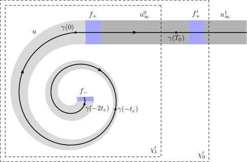
Figure 3. Concentration in phase space of the quasimode $\tilde{u}=u-\chi^{\prime}_{0}u^{0}_{\infty}-(1-\chi^{\prime}_{1})u^{1}_{\infty}$, showing its components $u$, $u_{\infty}^{0}$, $u_{\infty}^{1}$, the functions $f_{+},f_{-}$ from (5.1), the propagated function $f^{\prime}_{+}:=e^{-iT_{0}(P_{h}-\omega^{2})/h}f_{+}$, and the supports of the cutoffs $\chi^{\prime}_{0},\chi^{\prime}_{1}$. Here $t_{e}={\beta\over 2}\log(1/h)$ is just below the Ehrenfest time of the trajectory $\gamma$. Our construction is as follows: starting from a basic beam near $\gamma(-t_{e})$, we propagate it for times in $[-t_{e},t_{e}]$ to obtain $u$; see Figure 2. We next propagate $f_{+}$ forward for time $T_{0}$ which is large enough so that $P_{h}=-h^{2}\Delta_{g_{0}}$ on $\gamma([T_{0},\infty))$, to obtain $u_{\infty}^{0}$. We finally apply the free resolvent to $f^{\prime}_{+}$ to obtain $u_{\infty}^{1}$.

Since $\|f_{-}\|_{L^{2}}\leq Ch^{2\sqrt{E}\beta\nu}$, it remains to construct a function which compensates for the $f_{+}$ term in (5.1). This is done by the following

Lemma 5.1.

There exist $h$-dependent families of functions

$$u_{\infty}(x;h)\in C^{\infty}(M),\quad f_{\infty}(x;h)\in C_{0}^{\infty}(M)$$

such that for some $h$-independent constants $C,C_{\chi}$,

1. $u_{\infty}=hR_{h}(\omega)f_{\infty}$.

2. $f_{\infty}$ is supported inside some $h$-independent compact set.

3. $f_{\infty}=f_{+}+\mathcal{O}(h^{\infty})_{L^{2}}$.

4. $\|\chi u_{\infty}\|_{L^{2}}\leq C_{\chi}$ for each $\chi\in C_{0}^{\infty}(M)$, where $C_{\chi}$ depends on $\chi$.

5. $\operatorname{WF}_{h}(u_{\infty})\subset\gamma([t_{0}/3,\infty))$.

Proof.

Since $M$ is diffeomorphic to $\mathbb{R}^{n}$ outside of a compact set, we may write for $r_{0}>0$ large enough,

$$M=M_{r_{0}}\sqcup\big{(}\mathbb{R}^{n}\setminus\overline{B}(0,r_{0})\big{)},$$

where $\overline{B}(0,r_{0})\subset\mathbb{R}^{n}$ is the closed Euclidean ball of radius $r_{0}$ and $M_{r_{0}}\subset M$ is compact. We choose $r_{0}$ such that the potential $V$ is supported in $M_{r_{0}}$ and $g$ is equal to the Euclidean metric $g_{0}$ on $\mathbb{R}^{n}\setminus\overline{B}(0,r_{0})$; then

$$P_{h}=P_{h}^{0}\quad\text{on }\mathbb{R}^{n}\setminus\overline{B}(0,r_{0}),$$ (5.2)

where $P_{h}^{0}$ is the semiclassical Euclidean Laplacian on $\mathbb{R}^{n}$:

$$P_{h}^{0}=-h^{2}\Delta_{g_{0}}.$$

Since the trajectory $\gamma(t)$ escapes as $t\to+\infty$, there exists $T_{0}>0$ such that

$$M_{r_{0}}\cap\gamma\big{(}[T_{0},\infty)\big{)}=\emptyset.$$

We choose cutoff functions $\chi^{\prime}_{0},\chi^{\prime}_{1}\in C_{0}^{\infty}(M)$ such that (viewing them as functions on $T^{*}M$ if necessary)

$$\chi^{\prime}_{0}=1\quad\text{near }\gamma\big{(}(-\infty,T_{0}+t_{0}]\big{)},$$ (5.3)

$$\chi^{\prime}_{1}=1\quad\text{near }M_{r_{0}},$$ (5.4)

$$(\operatorname{supp}\chi^{\prime}_{1})\cap\gamma\big{(}[T_{0},\infty)\big{)}=\emptyset.$$ (5.5)

Consider the free resolvent

$$R^{0}_{h}(\omega)=(P_{h}^{0}-\omega^{2})^{-1}:L^{2}(\mathbb{R}^{n})\to L^{2}(\mathbb{R}^{n}),\quad\operatorname{Im}\omega>0;$$

we continue it meromorphically to a family of operators (see [DyZw, §3.1] or [Va, §7.2])

$$R^{0}_{h}(\omega):L^{2}_{\operatorname{comp}}(\mathbb{R}^{n})\to L^{2}_{\operatorname{loc}}(\mathbb{R}^{n}),\quad\omega\in\mathbb{C}.$$

We now define (see Figure 3)

$$u_{\infty} :=\chi^{\prime}_{0}u_{\infty}^{0}+(1-\chi^{\prime}_{1})u_{\infty}^{1},$$

$$u_{\infty}^{0} :=i\int_{0}^{T_{0}}e^{-it(P_{h}-\omega^{2})/h}f_{+}\,dt\ \in\ C^{\infty}(M),$$

$$u_{\infty}^{1} :=hR^{0}_{h}(\omega)(1-\chi^{\prime}_{1})\chi^{\prime}_{0}e^{-iT_{0}(P_{h}-\omega^{2})/h}f_{+}\ \in\ C^{\infty}(\mathbb{R}^{n}).$$

Since $\|f_{+}\|_{L^{2}}$ is bounded uniformly in $h$, so are $\|u_{\infty}^{0}\|_{L^{2}}$ and $\|\chi u_{\infty}^{1}\|_{L^{2}}$ for each $\chi\in C_{0}^{\infty}(\mathbb{R}^{n})$; the latter follows from boundedness of the free resolvent $R^{0}_{h}$ [DyZw, Theorem 3.1]. This proves part 4 of the lemma.

We next claim the following inclusions, which together imply part 5 of the lemma:

$$\operatorname{WF}_{h}(u_{\infty}^{0}) \ \subset\ \gamma\big{(}[t_{0}/3,T_{0}+2t_{0}/3]\big{)},$$ (5.6)

$$\operatorname{WF}_{h}(u_{\infty}^{1}) \ \subset\ \gamma\big{(}[T_{0}+t_{0}/3,\infty)\big{)}.$$ (5.7)

Indeed, by Lemma 4.1, $\operatorname{WF}_{h}(f_{+})\subset\gamma([t_{0}/3,2t_{0}/3])$; applying (2.5), we obtain

$$\operatorname{WF}_{h}(e^{-it(P_{h}-\omega^{2})/h}f_{+})\ \subset\ \gamma\big{(}[t+t_{0}/3,t+2t_{0}/3]\big{)}.$$ (5.8)

The inclusion (5.6) follows immediately. As for (5.7), it can be deduced from (5.8) for $t=T_{0}$ together with the following outgoing property of the resolvent $R_{h}^{0}(\omega)$, valid for each $h$-tempered family $f\in L^{2}_{\operatorname{comp}}(\mathbb{R}^{n})$:

$$\operatorname{WF}_{h}(R^{0}_{h}(\omega)f)\ \subset\ \bigcup_{t\geq 0}e^{tH_{p_{0}}}(\operatorname{WF}_{h}(f)),\quad p_{0}(x,\xi)=|\xi|_{g_{0}}^{2}.$$ (5.9)

The inclusion (5.9) follows from the oscillatory integral representation of $R^{0}_{h}(\omega)$ as in [DyZw, Lemma 3.52] combined with semiclassical propagation of singularities [Dy15, Proposition 3.4] for the operator $P_{h}^{0}-\omega^{2}$.

Now, we compute

$$(P_{h}-\omega^{2})u_{\infty}^{0} =-\int_{0}^{T_{0}}h\partial_{t}e^{-it(P_{h}-\omega^{2})/h}f_{+}\,dt=h(f_{+}-e^{-iT_{0}(P_{h}-\omega^{2})/h}f_{+}),$$

$$(1-\chi^{\prime}_{1})(P_{h}-\omega^{2})u_{\infty}^{1} =h(1-\chi^{\prime}_{1})^{2}\chi^{\prime}_{0}e^{-iT_{0}(P_{h}-\omega^{2})/h}f_{+},$$

where the last statement follows by (5.2).

Put

$$f_{\infty}:=h^{-1}(P_{h}-\omega^{2})u_{\infty},$$

then

$$f_{\infty}=\chi^{\prime}_{0}f_{+}+\chi^{\prime}_{0}\big{(}(1-\chi^{\prime}_{1})^{2}-1\big{)}e^{-iT_{0}(P_{h}-\omega^{2})/h}f_{+}+h^{-1}[P_{h},\chi^{\prime}_{0}]u_{\infty}^{0}-h^{-1}[P_{h},\chi^{\prime}_{1}]u_{\infty}^{1}.$$

Part 2 of the lemma follows from here immediately, and part 3 follows by analysing the terms on the right-hand side:

• the first term is equal to $f_{+}+\mathcal{O}(h^{\infty})_{L^{2}}$ by (5.3) and since $\operatorname{WF}_{h}(f_{+})\subset\gamma([t_{0}/3,2t_{0}/3])$;

• the second term is $\mathcal{O}(h^{\infty})_{L^{2}}$ by (5.5) and (5.8) for $t=T_{0}$;

• the third term is $\mathcal{O}(h^{\infty})_{L^{2}}$ by (5.3) and (5.6);

• and the fourth term is $\mathcal{O}(h^{\infty})_{L^{2}}$ by (5.5) and (5.7).

Finally, part 1 follows from the following two statements:

$$\chi^{\prime}_{0}u_{\infty}^{0} =R_{h}(\omega)(P_{h}-\omega^{2})\chi^{\prime}_{0}u_{\infty}^{0},$$ (5.10)

$$(1-\chi^{\prime}_{1})u_{\infty}^{1} =R_{h}(\omega)(P_{h}-\omega^{2})(1-\chi^{\prime}_{1})u_{\infty}^{1}.$$ (5.11)

The statement (5.10) follows from the identity

$$v=R_{h}(\omega)(P_{h}-\omega^{2})v,\quad v\in C_{0}^{\infty}(M),$$ (5.12)

which holds when $\operatorname{Im}\omega>0$ since $C_{0}^{\infty}(M)\subset L^{2}(M)$ and $R_{h}(\omega)$ is the inverse of $P_{h}-\omega^{2}$ on $L^{2}$, and for general $\omega$ by analytic continuation. The statement (5.11) follows from the identity

$$(1-\chi^{\prime}_{1})R^{0}_{h}(\omega)f=R_{h}(\omega)(P_{h}-\omega^{2})(1-\chi^{\prime}_{1})R^{0}_{h}(\omega)f,\quad f\in C_{0}^{\infty}(\mathbb{R}^{n}),$$

which is true for $\operatorname{Im}\omega>0$ since $(1-\chi^{\prime}_{1})R^{0}_{h}(\omega)f\in L^{2}(M)$ and for general $\omega$ by analytic continuation; here $(P_{h}-\omega^{2})(1-\chi^{\prime}_{1})R^{0}_{h}(\omega)f$ is compactly supported by (5.2). This finishes the proof of Lemma 5.1. ∎

We now finish the construction of the functions $\tilde{u},\tilde{f}$ and thus the proof of Theorem 1. Put

$$\tilde{u}:=u-u_{\infty},\quad\tilde{f}:=h^{-1}(P_{h}-\omega^{2})\tilde{u}=h^{-1}(P_{h}-\omega^{2})u-f_{\infty}.$$

Note that, since $u\in C_{0}^{\infty}(M)$, we have by (5.12)

$$u=R_{h}(\omega)(P_{h}-\omega^{2})u.$$

It follows that $\tilde{u}=hR_{h}(\omega)\tilde{f}$. Also, since both $u$ and $f_{\infty}$ are supported in some $h$-independent compact set, so is $\tilde{f}$. We next have by (5.1),

$$\tilde{f}=-f_{-}+\mathcal{O}(h^{\infty})_{L^{2}}=\mathcal{O}(h^{2\sqrt{E}\beta\nu})_{L^{2}}.$$

Finally, let $b\in S^{\operatorname{comp}}_{\rho}(T^{*}M)$ be the symbol from part 4 of Lemma 4.1. Then

$$\operatorname{WF}_{h}(\operatorname{Op}_{h}(b))\subset\gamma([-t_{0}/4,t_{0}/4]);$$

together with part 5 of Lemma 5.1, this implies that

$$\operatorname{Op}_{h}(b)u_{\infty}=\mathcal{O}(h^{\infty})_{L^{2}}.$$

Combining this with part 4 of Lemma 4.1, we see that

$$\|\operatorname{Op}_{h}(b)\tilde{u}\|_{L^{2}}\geq C^{-1}.$$

Since $\operatorname{Op}_{h}(b)$ is compactly supported in an $h$-independent set and its $L^{2}\to L^{2}$ norm is bounded uniformly in $h$, we obtain property (4) of $\tilde{u}$, finishing the proof.

References

- [BLR] Claude Bardos, Gilles Lebeau, and Jeffery Rauch, Sharp sufficient conditions for the observation, control, and stabilization of waves from the boundary, SIAM J. Control Optim. 30(1992), 1024–1065.
- [BBR] Jean-François Bony, Nicolas Burq, and Thierry Ramond, Minoration de la résolvante dans le cas captif, C. R. Math. 348(2010), 1279–1282.
- [BoPe] Jean-François Bony and Vesselin Petkov, Semiclassical estimates of the cut-off resolvent for trapping perturbations, J. Spectr. Theory 3(2013), 399–422.
- [BoRo] Jean-Marc Bouclet and Julien Royer, Local energy decay for the damped wave equation, J. Funct. Anal. 266(2014), 4538–4615.
- [BoTo] Alexander Borichev and Yuri Tomilov, Optimal polynomial decay of functions and operator semigroups, Math. Ann. 347(2010), 455–478.
- [BuCh] Nicolas Burq and Hans Christianson, Imperfect geometric control and overdamping for the damped wave equation, Comm. Math. Phys. 336(2015), 101–130.
- [BuGé] Nicolas Burq and Patrick Gérard, Condition nécessaire et suffisante pour la contrôlabilité exacte des ondes, C. R. Acad. Sci. Série I 325(1997), 749–752.
- [BuZu] Nicolas Burq and Claude Zuily, Concentration of Laplace eigenfunctions and stabilization of weakly damped wave equation, preprint, arXiv:1503.02058.
- [BuZw] Nicolas Burq and Maciej Zworski, Geometric control in the presence of a black box, Jour. Amer. Math. Soc. 17(2004), 443–471.
- [Ch08] Hans Christianson, Dispersive estimates for manifolds with one trapped orbit, Comm. PDE 33(2008), 1147–1174.
- [Ch09] Hans Christianson, Applications of cutoff resolvent estimates to the wave equation, Math. Res. Lett. 16(2009), 577–590.
- [Ch11] Hans Christianson, Quantum monodromy and nonconcentration near a closed semi-hyperbolic orbit, Trans. Amer. Math. Soc. 363(2011), 3373–3438.
- [ChMe] Hans Christianson and Jason Metcalfe, Sharp local smoothing for warped product manifolds with smooth inflection transmission, Indiana Univ. Math. J. 63(2014), 969–992.
- [ChWu] Hans Christianson and Jared Wunsch, Local smoothing for the Schrödinger equation with a prescribed loss, Amer. J. Math. 135(2013), 1601–1632.
- [CoRo] Monique Combescure and Didier Robert, Semiclassical spreading of quantum wave packets and applications near unstable fixed fixed points of the classical flow, Asympt. Anal. 14(1997), 377–404.
- [CoFe] Antonio Córdoba and Charles Fefferman, Wave packets and Fourier integral operators, Comm. Partial Differential equations 3(1978), 979–1005.
- [DDZ] Kiril Datchev, Semyon Dyatlov, and Maciej Zworski, Resonances and lower resolvent bounds, to appear in J. Spect. Th., arXiv:1402.0604.
- [DKLS] David Dos Santos Ferreira, Yaroslav Kurylev, Matti Lassas, and Mikko Salo, The Calderón problem in transversally anisotropic geometries, to appear in J. Eur. Math. Soc., arXiv:1305.1273.
- [Dy11] Semyon Dyatlov, Exponential energy decay for Kerr–de Sitter black holes beyond event horizons, Math. Res. Lett. 18(2011), 1023–1035.
- [Dy14] Semyon Dyatlov, Spectral gaps for normally hyperbolic trapping, to appear in Ann. Inst. Fourier, arXiv:1403.6401.
- [Dy15] Semyon Dyatlov, Resonance projectors and asymptotics for -normally hyperbolic trapped sets, J. Amer. Math. Soc. 28(2015), 311–381.
- [DyGu] Semyon Dyatlov and Colin Guillarmou, Microlocal limits of plane waves and Eisenstein functions, Ann. de l’ENS (4) 47(2014), 371–448.
- [DyZa] Semyon Dyatlov and Joshua Zahl, Spectral gaps, additive energy, and a fractal uncertainty principle, preprint, arXiv:1504.06589.
- [DyZw] Semyon Dyatlov and Maciej Zworski, Mathematical theory of scattering resonances, book in progress, http://math.mit.edu/~dyatlov/res/
- [EsNo] Suresh Eswarathasan an Stéphane Nonnenmacher, Strong scarring of logarithmic quasimodes, preprint; arXiv:1507.08371.
- [GrSj] Alain Grigis and Johannes Sjöstrand, Microlocal analysis for differential operators: an introduction, Cambridge University Press, 1994.
- [Ha] George Hagedorn, Semiclassical quantum mechanics IV. Large order asymptotics and more general states in more than one dimension, Ann. Inst. H. Poincaré Phys. Théor. 42(1985), 363–374.
- [HöIII] Lars Hörmander, The Analysis of Linear Partial Differential Operators III. Pseudo-Differential Operators, Springer, 1994.
- [KeSa] Carlos Kenig and Mikko Salo, The Calderón problem with partial data on manifolds and applications, Analysis&PDE 6(2013), 2003–2048.
- [LSV] Ari Laptev, Yuri Safarov, and Dmitry Vassiliev, On global representation of Lagrangian distributions and solutions of hyperbolic equations, Comm. Pure Appl. Math. 47(1994), 1411–1456.
- [LéLe] Matthieu Léautaud and Nicolas Lerner, Energy decay for a locally undamped wave equation, preprint, arXiv:1411.7271.
- [Le] Gilles Lebeau, Equation des ondes amorties, In A. Boutet de Monvel and V. Marchenko, editors, Algebraic and Geometric Methods in Mathematical Physics, 73–109, Kluwer Academic, The Netherlands, 1996.
- [LeRo] Gilles Lebeau and Luc Robbiano, Stabilisation de l’équation des ondes par le bord, Duke Math. J. 86(1997), 465–491.
- [NSZ] Shu Nakamura, Plamen Stefanov, and Maciej Zworski, Resonance expansions of propagators in the presence of potential barriers, J. Funct. Anal. 205(2003), 180–205.
- [NoZw] Stéphane Nonnenmacher and Maciej Zworski, Decay of correlations for normally hyperbolic trapping, Invent. Math. 200(2015), 345–438.
- [Po] M. M. Popov, A new method of computation of wave fields using Gaussian beams, Wave Motion, 4(1982), 85–97.
- [Ra69] James Ralston, Solutions of the wave equation with localized energy, Comm. Pure Appl. Math. 22(1969), 807–823.
- [Ra82] James Ralston, Gaussian beams and the propagation of singularities, Studies in partial differential equations, 206–248; MAA Stud. Math. 23(1982).
- [Sj] Johannes Sjöstrand, A trace formula and review of some estimates for resonances, Microlocal Analysis and Spectral Theory NATO ASI Series 490(1997), 377–437.
- [TaZw] Siu-Hung Tang and Maciej Zworski, From quasimodes to resonances, Math. Res. Lett. 5(1998), 261–272.
- [Va] Boris Vainberg, Asymptotic methods in equations of mathematical physics, Gordon and Breach, 1988.
- [Va13a] András Vasy, Microlocal analysis of asymptotically hyperbolic and Kerr–de Sitter spaces, with an appendix by Semyon Dyatlov, Invent. Math. 194(2013), 381–513.
- [Va13b] András Vasy, Microlocal analysis of asymptotically hyperbolic spaces and high energy resolvent estimates, Inverse Problems and Applications. Inside Out II, Gunther Uhlmann (ed.), MSRI publications 60, Cambridge Univ. Press, 2013.
- [WuZw] Jared Wunsch and Maciej Zworski, Resolvent estimates for normally hyperbolic trapped sets, Ann. Henri Poincaré, 12(2011), 1349–1385.
- [Zw] Maciej Zworski, Semiclassical analysis, Graduate Studies in Mathematics 138, AMS, 2012.