Kerr-de Sitter Greybody Factors via Isomonodromy

Abstract

Scattering data can be generically described in terms of monodromies. Here we obtain scattering amplitudes for conformally coupled scalar fields in Kerr-de Sitter black holes using this monodromy technique. The only non-trivial parameter, the composite monodromy parameter $\sigma_{ij}$ between two regular singular points, can be solved implicitily in terms of the Painlevé VI $\tau$-function. The application of the Virasoro conformal blocks to solve the latter can now be interpreted as a verification of the striking relationship between conformal symmetry and black holes.

1 Introduction

Scattering amplitudes are very important in the context of black hole physics. They relate directly to astrophysical problems but also to other theoretical problems like stability of gravitational solutions and AdS/CFT duality. Rotating black holes are particularly difficult to study and are usually treated using semi-analytical methods and matched asymptotic expansions.

Recent work have pointed to the possibility of extracting exact scattering amplitudes (in some particular cases) using only monodromy data of the radial part from the wave equation of interest Castro2013b ; Novaes:2014lha . In the latter work, the authors outlined a procedure to accomplish this program for conformally coupled scalars in a generic Kerr-NUT-(A)dS black hole. One of the results showed that the scattering amplitudes are completely determined by the composite monodromy parameter $\sigma$, and that the theory of isomonodromic flows Jimbo1981b ; Jimbo:1981-2 ; Jimbo:1981-3 exposes a hidden, non-linear symmetry of the parameters which can be used to relate the problem of finding $\sigma$ to the connection problem of the Painlevé VI transcendent. In this paper, we obtain explicit analytic expressions for $\sigma$ and the scattering coefficients using recent results for the Painlevé VI $\tau$-function expansion in terms of $c=1$ conformal blocks Gamayun:2012ma ; Gamayun:2013auu . We also show that both the scattering problem for the radial equation and the eigenvalue problem for angular equation can be solved by the isomonodromy method. Finally, we obtain the first corrections for $\sigma$ in both near-extremal Kerr-dS limits.

One important aspect of the master perturbation equation of spin $s$ fields for the Kerr-dS background - also called Teukolsky master equation (TME) - is that it is not only separable into radial and angular parts, but it can be reduced to a Fuchsian differential equation with 4 singular points Suzuki:1998vy . This equation has been studied since the late 19th century and it is called Heun’s differential equation when written in the canonical form:

$$y^{\prime\prime}+\left(\frac{\gamma}{z}+\frac{\delta}{z-1}+\frac{\epsilon}{z-t}\right)y^{\prime}+\frac{\alpha\beta z-q}{z(z-1)(z-t)}y=0,$$ (1)

with its coefficients obeying the Fuchs condition $\gamma+\delta+\epsilon=\alpha+\beta+1$. From this starting point, series expansions for scattering amplitudes in the Kerr-dS background have been obtained using a different method than ours by Suzuki, Takasugi and Umetsu in a series of papers Suzuki:1999nn ; Suzuki:1999pa . Inspired by earlier works of Erdélyi and Schmidt (for references, see the review book ronveaux1995heun ), Suzuki et al. used a hypergeometric series expansion for Heun functions:

$$y_{\nu}(z) =\sum_{n=-\infty}^{\infty}a^{\nu}_{n}\sideset{{}_{2}}{{}_{1}}{\operatorname*{F}}(-\nu-n-\tfrac{1}{2}+\tfrac{\kappa}{2},\nu+n+\tfrac{1}{2}+\tfrac{\kappa}{2};\gamma,z),$$ (2)

to study scattering in the Kerr-dS background. This series expansion converges with the correct local behaviour near $z=0$ and $z=1$ for special values of the coefficient $\nu$ coming from an augmented convergence condition.

The interpretation of $\nu$ is not so clear in the literature, but in the approach presented here its interpretation becomes quite natural: it is associated to the composite monodromy $\sigma_{ij}$ of the full solution around two singular points corresponding to the two horizons involved in the scattering. In particular, the series solution (2) has the correct local behaviour near $z=0$ – the outer horizon $r=r_{+}$ – and $z=1$ – the cosmological horizon $r=r_{C}$. The monodromy coefficient of (2) at $z=\infty$ is equal to the monodromy at infinity of the family of hypergeometric functions in (2), which is $\theta_{\infty}=2\nu+1\,(\text{mod}\,2n)$. With respect to the hypergeometric functions, this is equivalent to the composite monodromy of a loop enclosing $z=0$ and $z=1$ simultaneously and, therefore, $\nu$ parametrizes the composite monodromy between $0$ and $1$ of the full Heun solution (2).

Along with the obvious relevant applications for the scattering theory of black holes, the astrophysical and stability studies that issue from it, the extracting of the connection coefficients for the Heun equation described in this article is a century-old problem in mathematics, deeply tied to the Riemann-Hilbert problem. In its original form, this problem posed the question of writing an ordinary differential equation with prescribed monodromy data. As will be explained in Section 2, we will be primarily interested in the reverse Riemann-Hilbert problem, where one is interested in extracting the monodromy data from the differential equation. The major theoretical breakthroughs for solving this problem were achieved by Schlesinger, who discovered the non-linear symmetry of the monodromy data, encoded in the Schlesinger equations, which we will revise in Subsection 3.1. Another milestone came about with the work of Miwa, Jimbo and various collaborators, building up from critical systems in two-dimensional statistical mechanics Jimbo1981b ; Jimbo:1981-2 ; Jimbo:1981-3 , where the Hamiltonian structure of the Schlesinger equations (see Section 3) were explored to finally prove the Painlevé property of the solutions Miwa:1981 , fostering tremendous developments in integrable systems and the search for similar structures in other areas.

Another great leap came in from the AGT conjecture Alday:2009aq , its subsequent proof Alba:2010qc and the long series of applications to Painlevé transcendents, specially Gamayun:2012ma ; Gamayun:2013auu . In these combinatorial solutions for the Painlevé VI $\tau$-function were given exploring the relationship between accessory parameters of the Heun equation and four point functions in conformal field theories, via the Virasoro conformal blocks. We will give a very sketchy description of this relationship in Section 4. We will make the claim that this achieves the analytical solution of the scattering problem: an implicit solution for the scattering coefficients will be given in terms of the Painlevé VI $\tau$-function and the radial equation parameters. Likewise, the eigenvalue problem for the angular equation can also be cast in terms of monodromy data, yielding a formal solution, as explained in Appendix B. Both results are analytical and valid for generic ranges of black holes and scalar wave parameters, and we list expansions for the Painlevé VI $\tau$-function and scattering coefficients in Appendix A. The exploration of these solutions to extract physical intuition about black hole physics is a very interesting future problem.

The relationship between Fuchsian equations and the theory of special functions in the complex plane was clear since the beginning of the former field. The obvious ${\rm SL}(2,\mathbb{C})$ symmetry can be used to reduce some of the parameters, much in the way one can reduce the general Riemann differential equation to Gauss’s hypergeometric canonical form. What is perhaps less obvious is that one can use deep results from the Virasoro algebra representation theory to essentially solve the monodromy and connection problem for generic linear systems. We discuss the implications of this for scattering and black hole physics in Section 5. It is worth noting that, in a parallel result daCunha:2015ana , the authors gave analytical results for the standard asymptotically flat Kerr black hole in terms of the Painlevé V $\tau$-function, itself related to irregular conformal blocks.

Generic spin perturbations, described by the Teukolsky master equation Suzuki:1998vy , reduces to a differential equation of the same nature as eq. (1) and should be amenable to the same methods outlined here. In fact, this simplification happens for every vacuum type-D metric Batic2007 . Scalar fields in higher dimensional black holes backgrounds yield a more complicated isomonodronic structure, possibly tied to $W_{N}$ conformal blocks Gavrylenko:2015wla . More dimensions means more singular points and thus a higher-point isomonodromic flow. This case is not so well studied as the one with 4 singular points but it is known that the isomonodromic flow still has the Painlevé property Iwasaki:1991 and thus the asymptotics should be similar as in our case. Therefore, although we shall focus on scalar perturbations of $4$-dimensional Kerr-dS black holes, our method should be useful to understand the same integrable structure in more general cases for higher-spins and higher-dimensions.

2 Kerr-de Sitter Wave Equation

The metric of a 4-dimensional rotating black hole with de Sitter (dS) asymptotics has been obtained by Carter in the late 1960’s Carter:1968kx and the generalization for higher-dimensions, with the addition of a NUT charge, was found in Chen:2006qv . The special property that guided Carter to find this metric was the separability of the Hamilton-Jacobi equation for the geodesic motion. We now know that not only Hamilton-Jacobi but linear perturbation equations for this metric are also separable for spin 0, ${\frac{1}{2}}$, 1, $\tfrac{3}{2}$ and 2 Chambers:1994ap ; Suzuki:1998vy ; dias2012kerr , in the formalism of the Teukolsky master equation, which is true for any Petrov type-D spacetime. For convenience, the Kerr-dS metric can be written in Chambers-Moss coordinates as:

$$ds^{2}=-\frac{\Delta_{r}}{\rho^{2}\chi^{4}}\left(dt-a\sin^{2}\theta d\phi\right)^{2}+\frac{\Delta_{\theta}}{\rho^{2}\chi^{4}}\left(adt-(r^{2}+a^{2})d\phi\right)^{2}+\rho^{2}\left(\frac{d\theta^{2}}{\Delta_{\theta}}+\frac{dr^{2}}{\Delta_{r}}\right),$$ (3)

where $\chi^{2}=1+a^{2}/L^{2}$, with the dS radius $L^{2}=3/\Lambda$, and

$$\Delta_{\theta}=1+\frac{a^{2}}{L^{2}}\cos^{2}\theta,\quad\Delta_{r}=(r^{2}+a^{2})(1-\frac{r^{2}}{L^{2}})-2Mr,\quad\rho^{2}=r^{2}+a^{2}\cos^{2}\theta.$$ (4)

We have chosen the dS radius, but one can write the metric in terms of the AdS radius just by Wick rotating the radius $L\rightarrow iL$ and the Kerr metric can be recovered by making $L\rightarrow\infty$. The coordinate singularities of this metric are now given by the root of a 4th order polynomial $\Delta_{r}=0$. For a certain range of black hole parameters, we can find 4 real roots in the dS case, which we call $(r_{--},r_{-},r_{+},r_{C})$, and 2 real roots in the AdS case, called $(r_{-},r_{+},\zeta,\bar{\zeta})$. The roots $r_{-}$ and $r_{+}$ are the inner and outer horizon, respectively, like in the pure Kerr case. In the dS case, one of the roots is usually addressed as non-physical, $r_{--}=-(r_{+}+r_{-}+r_{C})$ is a negative number, and $r_{C}$ is the cosmological event horizon gibbons1977cosmological . To clarify the causal structure, we show the Penrose diagram of Kerr-dS for $\theta=0$ in Fig. 1. This diagram continues indefinitely in all directions.

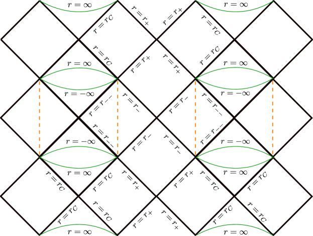
Figure 1: Causal diagram of maximally extended Kerr-dS black hole for $\theta=0$.

The dashed vertical line again represents the black hole singularity akcay2011kerr .

We define two Killing vectors:

$$\xi_{+}=\partial{t}+\Omega(r_{+})\partial{\phi},\quad\xi_{C}=\partial{t}+\Omega(r_{C})\partial{\phi},$$

such that they are null at each respective horizon $r_{+}$ and $r_{C}$. This entails to the constants $\Omega_{k}\equiv\Omega(r_{k})$ being the angular velocities of each horizon. In particular, this induces a frame-dragging effect near the event horizon, as no observer can stay stationary with respect to $\partial_{t}$ and is forced to co-rotate with the horizon. The angular velocity and temperatures of the event and cosmological horizons for an observer following $\xi_{k}$ orbits, with $k=C,+,-$, are given by:

$$\Omega_{k}=\frac{a}{r_{k}^{2}+a^{2}},\quad T_{k}=\frac{|\Delta_{r}^{\prime}(r_{k})|}{4\pi\chi^{2}(r_{k}^{2}+a^{2})},$$ (5)

in which we choose the sign of $T_{k}$ to both be positive temperatures.

Let $\psi(t,\phi,r,\theta)=e^{-i\omega t}e^{im\phi}R(r)S(\theta)$ be a solution of the Klein-Gordon equation for $D=4$ Kerr-dS metric in Chambers-Moss coordinates (3). The radial equation resulting from this solution is:

$$\partial_{r}(\Delta_{r}\partial_{r}R(r))+\left(-\frac{12\xi}{L^{2}}r^{2}+\frac{\chi^{4}(\omega(r^{2}+a^{2})-am)^{2}}{\Delta_{r}}\right)R(r)=C_{\ell}R(r),$$ (6)

where the separation constant between the angular and radial equations is $C_{\ell}=\lambda_{\ell}+\chi^{2}(a^{2}\omega^{2}-2ma\omega)$. The parameter $\xi$ is the coupling constant between the scalar field and the Ricci scalar. Typical values of the parameter $\xi$ are minimal coupling $\xi=0$ and conformal coupling $\xi=1/6$. In the latter, (6) is equivalent to the Teukolsky master equation for a spin zero perturbation Suzuki:1998vy ; Suzuki:1999nn . The angular equation has essentially the same form as the radial one and we are also able to obtain formally the $\lambda_{\ell}$ eigenvalues with the method outlined below, as described in the Appendix B.

If we restrict to the conformally coupled case, the equation (6) can be reduced to a Heun equation Suzuki:1998vy ; Batic2007 ; Novaes:2014lha :

$$y^{\prime\prime}(z)+\left(\frac{1-\theta_{0}}{z}+\frac{1-\theta_{1}}{z-1}+\frac{1-\theta_{t_{0}}}{z-t_{0}}\right)y^{\prime}(z)+\left(\frac{q_{1}q_{2}}{z(z-1)}-\frac{t_{0}(t_{0}-1)K_{0}}{z(z-1)(z-t_{0})}\right)y(z)=0,$$ (7)

where $y(z)$ is given in terms of $R(r)$ by:

$$y(z)=z^{\theta_{0}/2}(z-1)^{\theta_{1}/2}(z-t_{0})^{\theta_{t_{0}}/2}(z-z_{\infty})^{-1}R(r);$$ (8)

and

$$z=z_{\infty}\frac{r-r_{-}}{r-r_{--}},\quad z_{\infty}=\frac{r_{C}-r_{--}}{r_{C}-r_{-}},\quad t_{0}=z_{\infty}\frac{r_{+}-r_{-}}{r_{+}-r_{--}}.$$ (9)

We note that the scalar Teukolsky master equation is equivalent to the Klein-Gordon equation for a conformally coupled massless scalar field. The monodromy coefficients are

$$\theta_{k} =2i\chi^{2}\left(\frac{\omega(r_{k}^{2}+a^{2})-am}{\Delta_{r}^{\prime}(r_{k})}\right)=\pm\frac{i}{2\pi}\left(\frac{\omega-\Omega_{k}m}{T_{k}}\right),\quad k=0,1,t_{0},\infty,$$ (10)

where we use plus or minus sign to have positive temperatures $$T_{k}$$, and

$$K_{0} =-\frac{1}{t_{0}-z_{\infty}}\left[1+\frac{r_{+}-r_{--}}{\Delta_{r}^{\prime}(r_{+})}\left(-\frac{2}{L^{2}}r_{+}^{2}+\lambda_{\ell}+\chi^{2}(a^{2}\omega^{2}-2a\omega m)\right)\right.$$

$$\qquad\qquad\qquad\left.-2i\chi^{2}\frac{\omega(r_{+}r_{--}+a^{2})-am}{\Delta^{\prime}_{r}(r_{+})}\right].$$ (11)

The values of $\theta_{k}$ obey Fuchs relation $\theta_{0}+\theta_{1}+\theta_{t_{0}}+q_{1}+q_{2}=2$ and $q_{2}-q_{1}=\theta_{\infty}$. Also, in terms of (7), we have that $q_{1}q_{2}=1+\theta_{\infty}$. The set of 7 parameters $(\theta_{0},\theta_{1},\theta_{t_{0}},\kappa_{1},\kappa_{2};t_{0},K_{0})$ in (7) are related by the Fuchs relation, and we see that the resulting 6 parameters define the Heun equation and its fundamental solutions. The Heun equation has a rich history in mathematical physics. For such details about it, we refer to ronveaux1995heun ; slavyanov2000 .

The Riemann symbol for (7) is

$$y(z)={\rm P}\left\{\begin{array}[]{ccccc}0&1&t_{0}&\infty&\\ 0&0&0&q_{1}&z\\ \theta_{0}&\theta_{1}&\theta_{t_{0}}&q_{2}&\end{array}\right\},$$ (12)

and the parameters (10) and (2) are complex, so it is not trivial that, given a solution $y(z)$, the complex conjugate $(y(z))^{*}$ will also be a solution. However, it can be checked that $(y(z))^{*}$ satisfies (7) with parameters $(-\theta_{0},-\theta_{1},-\theta_{t_{0}};t_{0},K_{0}^{*})$, when the physical parameters are real – note that $t_{0}$ is real in the de Sitter case. More importantly, the radial part of the field $R(r)$ behaves in a well-determined manner under time-reversal

$$T[R_{\omega,\ell,m}(r)]=R_{-\omega,\ell,-m}(r).$$ (13)

Thus, $y(z)$ and its complex conjugate are also related by time-reversal. This can be checked by inspecting the transformation that brings the radial equation (6) to the canonical form (7). If one invert the signs of the $\theta_{i}$’s in (8), one arrives at the ODE satisfied by $(y(z))^{*}$. Hence, time-reversion symmetry tells us that a set of linearly independent solutions of (7) is:

$$y(z)\quad\text{and}\quad z^{\theta_{0}}(z-1)^{\theta_{1}}(z-t_{0})^{\theta_{t_{0}}}(y(z))^{*}.$$ (14)

Note that the Riemann symbol for both solutions are the same. This fact will be important below when trying to compute the scattering coefficients in terms of connection data.

3 Isomonodromic Approach to the Scattering Problem

Consider now two linearly independent solutions $y^{(1)}(z)$ and $y^{(2)}(z)$ of (7). The connection problem for the ODE consists in writing a solution with known behavior near one singular point, $y_{i}^{(1)}(z)$ at $z=z_{i}$, as the particular linear combination of solutions with known behavior at another critical point $z=z_{j}$,

$$y_{i}^{(1)}(z)=(E_{ij})_{11}y_{j}^{(1)}(z)+(E_{ij})_{12}y_{j}^{(2)}(z).$$ (15)

Along with the connection coefficients $(E_{ij})_{11}$ and $(E_{ij})_{12}$ for $y_{i}^{(1)}(z)$ there are the supplementary connection coefficients $(E_{ij})_{21}$ and $(E_{ij})_{22}$ for the linearly independent solution $y_{i}^{(2)}(z)$ with known behavior at $z=z_{i}$. So the $E_{ij}$ should really be thought of as matrices.

Solving the connection problem is intimately related to the monodromy problem. For Fuchsian equations, the independent solutions with known behavior at $z=z_{i}$ are of the form:

$$y^{\{1,2\}}_{i}(z)=(z-z_{i})^{\alpha_{i}^{\{1,2\}}}(1+{\cal O}(z-z_{i}))$$ (16)

where $\alpha^{\{1,2\}}_{i}$ are the solutions of the indicial equation at $z_{i}$. Because in general these are non-integers, we have that $y^{\{1,2\}}_{i}(e^{2\pi i}(z-z_{i})+z_{i})=e^{2\pi i\alpha_{i}^{\{1,2\}}}y^{\{1,2\}}_{i}(z)$. The matrix

$$D_{i}=\left(\begin{array}[]{cc}e^{2\pi i\alpha_{i}^{1}}&0\\ 0&e^{2\pi i\alpha_{i}^{2}}\end{array}\right)$$ (17)

implements the effect of this monodromy around the solutions with known behavior at $z_{i}$. If, however, we decide to write the matrix $D_{i}$ not in terms of $y^{\{1,2\}}_{i}(z)$ but in terms of $y^{\{1,2\}}_{j}(z)$, we will have to conjugate it using the connection matrix:

$$M_{ij}=E_{ij}D_{j}(E_{ij})^{-1},$$ (18)

where $M_{ij}$ is now the matrix associated to the monodromy around $z_{i}$ written in the natural basis for $z_{j}$ – i.e., those obtained by the Frobenius method from the solutions of the indicial equation, where the monodromy around $z_{j}$ is diagonal.

It is clear now that if we use another basis, not necessarily one associated to a critical point, the matrix $M_{i}$ associated to the monodromy around $z_{i}$ will be related to $M_{ij}$ by conjugation. Solving the monodromy problem amounts to find the set of $M_{i}$ associated to monodromies around all singular points of a known ODE. This is the reverse of the Riemann-Hilbert problem (in its initial guise), which is to write an ODE with a known set of monodromy matrices $M_{i}$. For Fuchsian equations with up to three regular singular points, the $M_{i}$ – and hence the $E_{ij}$ up to normalization – are completely determined from the solutions of the indicial parameters $\alpha_{i}^{\{1,2\}}$, information readily available from the ODE. For four or more regular singular points, the $M_{i}$ depend in a very non-trivial way on the accessory parameters, which in the Heun equation case (7) is essentially related to $t_{0}$ and $K_{0}$. When there are irregular singular points, Stokes parameters also come into play Castro2013b ; Jimbo1981b . This happens for the scalar wave equation of the Kerr black hole and we treat this problem in a separate paper daCunha:2015ana .

Also, a simple parameter counting argument shows that we cannot have all possible sets of $M_{i}$ represented by the initial ODE - we have to introduce apparent singularities Iwasaki:1991 . So, instead of studying the Riemann-Hilbert problem from the ODE perspective, it is more illuminating to use a matricial system:

$$\frac{d}{dz}\Phi(z)=A(z)\Phi(z),$$ (19)

where

$$A(z)=\begin{pmatrix}A_{11}&A_{12}\\ A_{21}&A_{22}\end{pmatrix}=\sum_{i}\frac{A_{i}}{z-z_{i}},$$ (20)

with $A_{i}$ being matrices independent of $z$. Each row of the matrix

$$\Phi(z)=\begin{pmatrix}y^{(1)}(z)&y^{(2)}(z)\\ w^{(1)}(z)&w^{(2)}(z)\end{pmatrix}$$ (21)

consists of linearly independent solutions of the ODEs below. This matricial system is generically called a Fuchsian system. It can be easily verified that any element of the first row of $\Phi(z)$ will satisfy the ODE:

$$\partial_{z}^{2}y-(\operatorname{Tr}A+\partial_{z}\log A_{12})\partial_{z}y+(\det A-\partial_{z}A_{11}+A_{11}\partial_{z}\log A_{12})y=0,$$ (22)

whereas elements of the second row will satisfy a similar equation, but with indices $1$ and $2$ interchanged:

$$\partial_{z}^{2}w-(\operatorname{Tr}A+\partial_{z}\log A_{21})\partial_{z}w+(\det A-\partial_{z}A_{22}+A_{22}\partial_{z}\log A_{21})w=0.$$ (23)

It is also straightforward that the elements of a given row will be linearly independent. The respective Wronskians for (22) and (23) are:

$$W_{1}(z)=A_{12}(z)\operatorname{Det}\Phi(z),\quad\quad W_{2}(z)=A_{21}(z)\operatorname{Det}\Phi(z),$$ (24)

and theorems of existence and unicity of solutions tells us that any two solutions $\Phi^{(1)}(z)$ and $\Phi^{(2)}(z)$ of the Fuchsian system are related by right multiplication by a constant matrix $g$, i.e, $\Phi^{(1)}(z)=\Phi^{(2)}(z)g$.

The Fuchsian system connects the Riemann-Hilbert problem with the theory of flat holomorphic connections Atiyah:1982 . From equation (19) for $\Phi(z)$, we see that:

$$A(z)=\frac{d\Phi(z)}{dz}\Phi^{-1}(z),$$ (25)

which suggests the interpretation of $A(z)$ as a flat ${\rm GL(2,\mathbb{C})}$ connection. Clearly, $\Phi(z)$ is uniquely defined by an initial condition $\Phi(z_{0})=\Phi_{0}$ and changing the condition amounts to a conjugation transformation $\tilde{\Phi}(z)=\Phi(z)g$, for $g\in{\rm GL}(2,\mathbb{C})$. The formal solution for $\Phi(z)$ above is

$$\Phi(z)=\mathcal{P}\exp\left(\int^{z}_{z_{0}}A(z)dz\right)\,\Phi_{0},$$ (26)

therefore, the poles of $A(z)$ correspond to the branch points of $\Phi(z)$. We thus see that the monodromy problem can be recast as a holonomy problem of the connection $A(z)$.

We will now set the parameters of $A_{i}$ so that the equation (22) mimics the Heun equation (7). Given the system (19) with 4 regular singular points in the canonical gauge, we parametrize the $A_{i}$ following Jimbo:1981-2 :

$$A_{i}=\begin{pmatrix}p_{i}+\theta_{i}&-q_{i}p_{i}\\ \frac{1}{q_{i}}(p_{i}+\theta_{i})&-p_{i}\end{pmatrix},\quad i=0,1,t,$$ (27)

so that

$$A_{\infty}=-(A_{0}+A_{1}+A_{t})=\begin{pmatrix}\kappa_{1}&0\\ 0&\kappa_{2}\end{pmatrix},\quad\theta_{i}=\operatorname{Tr}A_{i},\quad\theta_{i}^{2}=\operatorname{Tr}A_{i}^{2},$$ (28)

and

$$A_{12}=k\frac{z-\lambda}{z(z-1)(z-t)},\quad k\in\mathbb{C},$$ (29)

with $\lambda$ being a complicated function of the $p_{i}$ and $q_{i}$. With this parametrization, we can find that each first row element of $\Phi(z)$ satisfy

$$y^{\prime\prime}+p(z,t)y^{\prime}+q(z,t)y=0,$$ (30a)

$$p(z,t)=\frac{1-\theta_{0}}{z}+\frac{1-\theta_{1}}{z-1}+\frac{1-\theta_{t}}{z-t}-\frac{1}{z-\lambda},$$ (30b)

$$q(z,t)=\frac{\kappa_{1}(\kappa_{2}+1)}{z(z-1)}-\frac{t(t-1)K}{z(z-1)(z-t)}+\frac{\lambda(\lambda-1)\mu}{z(z-1)(z-\lambda)},$$ (30c)

where $\mu$ is $A_{11}(z)$ calculated at $z=\lambda$. By setting $\lambda=t$, $\theta_{t}=\theta_{t_{0}}-1$ and $-\mu+K=K_{0}$, we can recover (7) by making $t=t_{0}$. An explicit parametrization is given by

$$\begin{gathered}p_{0}=-\frac{(\theta_{0}+\theta_{1}-\theta_{t}+\theta_{\infty})(\theta_{0}-\theta_{1}+(1+2t_{0})\theta_{t}+\theta_{\infty})}{4\theta_{\infty}}+\frac{t_{0}(t_{0}-1)}{\theta_{\infty}}\left(K_{0}+\frac{\theta_{0}\theta_{t}}{t_{0}}+\frac{\theta_{1}\theta_{t}}{t_{0}-1}\right),\\[5.0pt] p_{1}=\frac{(\theta_{0}+\theta_{1}-\theta_{t}+\theta_{\infty})(\theta_{0}-\theta_{1}+(1+2t_{0})\theta_{t}-\theta_{\infty})}{4\theta_{\infty}}-\frac{t_{0}(t_{0}-1)}{\theta_{\infty}}\left(K_{0}+\frac{\theta_{0}\theta_{t}}{t_{0}}+\frac{\theta_{1}\theta_{t}}{t_{0}-1}\right),\\[5.0pt] (A_{t})_{21}=-\frac{p_{0}+\theta_{0}}{q_{0}}-\frac{p_{1}+\theta_{1}}{q_{1}},\quad\quad p_{t}=-\theta_{t},\quad\quad q_{0}=-\frac{p_{1}}{p_{0}}q_{1},\quad\quad q_{t}=0,\end{gathered}$$ (31)

where $\theta_{\infty}=\kappa_{1}-\kappa_{2}$. Even with these choices, there is still some freedom in choosing the elements of $A(z)$ given the ODE, since the value of $q_{0}$ and $q_{1}$ is determined up to a multiplicative factor. From the ODE (22), it is clear that

$$A(z)\quad\text{and}\quad e^{-q\sigma_{3}}A(z)e^{q\sigma_{3}},$$ (32)

with $q$ some arbitrary complex constant, will yield the same ODE for both rows of $\Phi$. In terms of the parametrization (27) this corresponds to an overall scaling of the $q_{i}$’s, or still a rescaling of $k$ in $A_{12}$. We will use this freedom below to fix the normalization of the solution. Note that this transformation maintains the Wronskian invariant.

The boundary conditions associated with the Fuchsian system with the choice (28) are schematically given by

$$\Phi(z)=\begin{cases}G_{i}(\mathbbold{1}+{\cal O}(z-z_{i}))(z-z_{i})^{\left(\begin{smallmatrix}\theta_{i}&0\\ 0&0\end{smallmatrix}\right)}g_{i},\quad\quad z\rightarrow z_{i},\\ (\mathbbold{1}+{\cal O}(z^{-1}))z^{-\left(\begin{smallmatrix}\kappa_{1}&0\\ 0&\kappa_{2}\end{smallmatrix}\right)},\quad\quad z\rightarrow\infty,\end{cases}$$ (33)

where

$$G_{i}=\lambda_{i}\begin{pmatrix}q_{i}&1\\ 1&\frac{p_{i}+\theta_{i}}{q_{i}p_{i}}\end{pmatrix}e^{\beta_{i}\sigma_{3}}$$ (34)

and $g_{i}$ are the connection matrices, to be discussed below. Explicitly, we have $G_{i}$ as the most general matrix such that $A_{i}=G_{i}\left(\begin{smallmatrix}\theta_{i}&0\\ 0&0\end{smallmatrix}\right)G_{i}^{-1}$. With this parametrization, we define the canonical – or “natural” – solutions near $z_{i}$ to be $\Phi_{i}(z)\equiv\Phi(z)g_{i}^{-1}$ and note the leading behavior for each entry of $\Phi_{i}(z)$, based on the parametrization for $G_{i}$,

$$y^{(1)}_{i}(z) =\lambda_{i}e^{\beta_{i}}q_{i}(z-z_{i})^{\theta_{i}}(1+\ldots),\quad\quad y^{(2)}_{i}(z) =\lambda_{i}e^{-\beta_{i}}(1+\ldots),$$ (35)

$$w^{(1)}_{i}(z) =\lambda_{i}e^{\beta_{i}}(z-z_{i})^{\theta_{i}}(1+\ldots),\quad\quad w^{(2)}_{i}(z) =\lambda_{i}e^{-\beta_{i}}\frac{p_{i}+\theta_{i}}{q_{i}p_{i}}(1+\ldots),$$

where we are disregarding ${\cal O}(z-z_{i})$ subleading terms in both Frobenius expansions. The values of $\lambda_{i}$ are determined from boundary conditions once we fix that the connection matrices should satisfy $\det g_{i}=1$. Given that one can choose boundary conditions such that

$$W(z)\equiv\det\Phi(z)=z^{\theta_{0}}(z-t_{0})^{\theta_{t_{0}}-1}(z-1)^{\theta_{1}},$$ (36)

then, for $\det g_{i}=1$, we compare the asymptotic expressions (35) and find

$$\lambda_{i}^{2}=\frac{p_{i}}{\theta_{i}}\prod_{j\neq i}(z_{i}-z_{j})^{\theta_{j}}.$$ (37)

We will fix the real part of the $\beta_{i}$ by requiring that $y_{i}^{(1,2)}(z)$ in (35) are associated with equal but opposite radiation fluxes. The radial equation has real coefficients, then if $R(r)$ is a solution of (6), so is its complex conjugate $R^{*}(r)$. One can then easily find that the quantity

$$\mathcal{J}=-i\frac{\Delta_{r}(r)}{\Delta^{\prime}_{r}(r_{--})}\left(R^{*}(r)\frac{d}{dr}R(r)-R(r)\frac{d}{dr}R^{*}(r)\right)$$ (38)

is independent of $r$ if $R(r)$ is a solution of (6). Physically, this corresponds to the radiation flux in the $r$ direction, with a prefactor chosen for later convenience. In terms of $y(z)$ and $y^{*}(z)$, (38) becomes

$$\mathcal{J} =\begin{aligned} if(z)&\left[W(z)^{1/2}y^{*}(z)\frac{d}{dz}\left(W(z)^{-1/2}y(z)\right)\right.\\ &\left.\qquad-W(z)^{-1/2}y(z)\frac{d}{dz}\left(W(z)^{1/2}y^{*}(z)\right)\right]\end{aligned}$$ (39)

$$=if(z)\left\{\hat{W}[y,y^{*}]-\frac{W^{{}^{\prime}}}{W}|y|^{2}\right\}$$ (40)

where $f(z)=z(z-1)(z-t_{0})$ and $\hat{W}[y_{1},y_{2}]=y_{1}y_{2}^{\prime}-y_{2}y_{1}^{\prime}$ is the Wronskian of two functions. Near $z=1$, we find that

$$e^{\beta_{1}+\beta_{1}^{*}}=\frac{1}{|q_{1}|},$$ (41)

and thus the value of $\mathcal{J}^{(2)}=-\mathcal{J}^{(1)}$ is

$$\mathcal{J}^{(2)}=\left|p_{1}q_{1}\right|,$$ (42)

which is independent of $z$ and then will allow us to compare the normalization of the solutions $y_{i}^{(1,2)}(z)$ at different points. One can repeat this calculation for the solutions near $z=t$, for example, and check that the same answer as above is obtained.

The scattering problem is formulated in terms of the normalized radial wavefunctions $u_{i}^{\pm}$, for example,

$$u_{t}^{-}(r)=\frac{1}{{\cal T}}u_{1}^{-}(r)+\frac{{\cal R}}{{\cal T}}u_{1}^{+}(r),$$ (43)

where $u_{t}^{-}(r)$ represents a normalized purely incoming wave at the black hole outer horizon $z=t$ and $u^{\pm}_{1}(r)$ represent normalized incoming and outgoing waves at the cosmological horizon $z=1$. The problem is complemented by its time-reversed version

$$u^{+}_{t}(r)=\frac{{\cal R}^{\prime}}{{\cal T}^{\prime}}u_{1}^{-}(r)+\frac{1}{{\cal T}^{\prime}}u_{1}^{+}(r),$$ (44)

where a purely outgoing wave at the black hole horizon divides into a superposition of incoming and outgoing waves at the cosmological horizon. We can now fix $k$ in (29) and the scattering coefficients in such a way that $y^{(1)}_{t}$ corresponds to $u^{-}_{t}(r)$ and $y^{(2)}_{t}$ to $u^{+}_{t}(r)$. With this provision, we can see that the normalized connection matrix between $z=t$ and $z=1$ is of the form:

$$E_{t1}=g_{t}g_{1}^{-1}=\begin{pmatrix}\frac{1}{{\cal T}}&\frac{{\cal R}^{\prime}}{{\cal T}^{\prime}}\\ \frac{{\cal R}}{{\cal T}}&\frac{1}{{\cal T}^{\prime}}\end{pmatrix},$$ (45)

which simplifies our calculations somewhat because we will not need the full set of monodromy matrices to compute the scattering coefficients. Now, consider the composite monodromy $\sigma_{1t}$ defined by

$$2\cos\pi\sigma_{1t}=\operatorname{Tr}(M_{1}M_{t}).$$ (46)

The monodromy matrix around $z=z_{i}$ can be written as $M_{i}=g_{i}^{-1}D_{i}g_{i}$. Plugging this into (46) and, using (45), we find that

$$\mathcal{T}\mathcal{T}^{\prime}=\frac{2\sin\pi\theta_{1}\sin\pi\theta_{t}}{\cos\pi(\theta_{1}-\theta_{t})-\cos\pi\sigma_{1t}}=\frac{\sin\pi\theta_{1}\sin\pi\theta_{t}}{\sin\frac{\pi}{2}(\sigma_{1t}+\theta_{1}-\theta_{t})\sin\frac{\pi}{2}(\sigma_{1t}-\theta_{1}+\theta_{t})}.$$ (47)

Therefore, the scattering amplitudes only depend on the monodromy data. When $\sigma_{1t}$ is either real or purely imaginary, (47) is real and we have a well-defined scattering problem with $u_{t}^{+}$ being the complex conjugate of $u_{t}^{-}$. However, when $\sigma_{1t}$ is complex, we notice that the amplitudes are defined up to a phase. Therefore, we set

$$\mathcal{T}^{\prime}=\mathcal{T}^{*}e^{i\phi}$$ (48)

and this extra phase can be absorbed in the imaginary part of $\beta_{t}$ in (35), for example, which is not fixed a priori by our radiation flux argument. Finally, we end with

$$|\mathcal{T}|^{2}=\left|\frac{\sin\pi\theta_{1}\sin\pi\theta_{t}}{\sin\frac{\pi}{2}(\sigma_{1t}+\theta_{1}-\theta_{t})\sin\frac{\pi}{2}(\sigma_{1t}-\theta_{1}+\theta_{t})}\right|.$$ (49)

Now, the only non-trivial global information we cannot read directly from the ODE is the composite monodromy parameter $\sigma_{1t}$, which is not easy to calculate from (7). This is the subject of the following section.

Even without a deep study of the parameter $\sigma_{1t}$, one can learn some lessons from the general structure of the formula for the transmission coefficient (49). First and foremost, superradiance occurs for frequencies $\omega$ and azimuthal angular momentum $m$ in the range where both $\theta_{t_{0}}$ and $\theta_{1}$ are (imaginary) negative:

$$\theta_{t_{0}}=\frac{i}{2\pi}\frac{\omega-\Omega_{+}m}{T_{+}},\quad\quad\theta_{1}=\frac{i}{2\pi}\frac{\omega-\Omega_{C}m}{T_{C}}$$ (50)

and quasi-normal modes are found from the vanishing of the denominator, which poses a quantization condition for $\sigma_{1t}$,

$$\sigma_{1t}\pm(\theta_{1}-\theta_{t})=2\pi n,\quad\quad n\in\mathbb{Z}.$$ (51)

Similar conditions also hold for the inner-outer horizon quasi-normal modes. The impact of these results for the general problem of inner horizon instabilities will be left for future work.

3.1 Isomonodromic Deformations

The isomonodromic deformation of (22) is a non-linear symmetry with an interesting interpretation in terms of flat holomorphic connections and transcendental functions. We have previously pointed out Novaes:2014lha the importance of this symmetry to the analytical solution of the scattering problem, and refer to it for a review on the subject. Following Jimbo:1981-2 ; Jimbo:1981-3 ; Jimbo1981b ; Iwasaki:1991 , if we take the partial fraction expansion of $A(z)$ then the system

$$A(z,t)=\frac{A_{0}}{z}+\frac{A_{1}}{z-1}+\frac{A_{t}}{z-t},\quad\quad B(z,t)=-\frac{A_{t}}{z-t}$$ (52)

represents the components of a flat holomorphic connection in the two-dimensional complex space $z,t$, satisfying $\partial_{z}A-\partial_{t}B-[A,B]=0$ if $A_{i}$ satisfies the Schlesinger equations:

$$\begin{gathered}\frac{\partial A_{0}}{\partial t}=\frac{1}{t}[A_{t},A_{0}],\quad\quad\frac{\partial A_{1}}{\partial t}=\frac{1}{t-1}[A_{t},A_{1}],\\[5.0pt] \frac{\partial A_{t}}{\partial t}=\frac{1}{t}[A_{0},A_{t}]+\frac{1}{t-1}[A_{1},A_{t}].\end{gathered}$$ (53)

Given that the connection is flat, we have that, along the solutions of the Schlesinger equations with respect to the flow of $t$, the monodromy data is the same – the matrices $M_{i}$ are mantained up to overall conjugation. This warrants the name “isomonodromic deformation” for the solutions of the Schlesinger equations.

Let us write the Schlesinger equations for the corresponding differential equation (30). The singularity at $z=\lambda$ in (30) is known as an apparent singularity, because its monodromy is trivial. This implies in an algebraic constraint between $K$, $\lambda$ and $\mu$, which will be explicited below. The parameters $\mu$ and $\lambda$ can be seen as canonically conjugate variables if the Schlesinger equations are written as the Hamiltonian system:

$$\begin{gathered}\frac{d\lambda}{d{t}}=\{K,\lambda\},\quad\quad\frac{d\mu}{d{t}}=\{K,\mu\},\\[10.0pt] K(\lambda,\mu,t)=\frac{\lambda(\lambda-1)(\lambda-t)}{t(t-1)}\left[\mu^{2}-\left(\frac{\theta_{0}}{\lambda}+\frac{\theta_{1}}{\lambda-1}+\frac{\theta_{t}-1}{\lambda-t}\right)\mu+\frac{\kappa_{1}(\kappa_{2}+1)}{\lambda(\lambda-1)}\right],\end{gathered}$$ (54)

with the canonical Poisson bracket $\{f,g\}=\frac{\partial f}{\partial\mu}\frac{\partial g}{\partial\lambda}-\frac{\partial f}{\partial\lambda}\frac{\partial g}{\partial\mu}$.

This Hamiltonian system can be used in principle to calculate the monodromy data, but as it turns out (54) can only be solved in general in terms of the Painlevé VI transcendent, whose general properties are still unknown Guzzetti2011 , but are under active study given its relation to the AGT relation in Liouville field theory Gamayun:2013auu ; Iorgov:2013uoa ; Iorgov:2014vla . The problem immediately relevant to us is to extract the monodromy parameter $\sigma_{1t}$ (46) from the asymptotics of the Painlevé system. The system is determined by (54) with initial data:

$$\mu(t_{0})=-\frac{K_{0}}{\theta_{t}},\quad\quad\lambda(t_{0})=t_{0},$$ (55)

and one can read $\sigma$ from the asymptotics of the isomonodromic flow near $t=1$ Jimbo:1982 ; Guzzetti2011 :

$$\lambda=1+\eta(t-1)^{1-\sigma_{1t}}+\ldots$$ (56)

valid when $0\leq\Re\sigma_{1t}<1$. This particular asymptotic behavior at $t=1$ will be clarified in the next section. The constant $\eta$ is related to the other monodromy parameter $\operatorname{Tr}(M_{0}M_{t})$ albeit by a complicated expression Novaes:2014lha .

Asymptotics are more easily obtained for the $\tau$-function, defined as:

$$\frac{d}{dt}\log\tau(t,\vec{\theta},\vec{\sigma})=\frac{1}{t}\operatorname{Tr}(A_{0}A_{t})+\frac{1}{t-1}\operatorname{Tr}(A_{1}A_{t}),$$ (57)

which is related to the parameters of the dynamical system $K,\mu,\lambda$ by

$$\frac{d}{dt} \log\tau(t,\{\theta_{i}\})=K(\lambda,\mu,t)+\frac{\theta_{0}\theta_{t}}{t}+\frac{\theta_{1}\theta_{t}}{t-1}-\frac{\kappa_{1}(\lambda-t)}{t(t-1)}-\frac{\lambda(\lambda-1)\mu}{t(t-1)}$$ (58)

$$=\frac{\lambda(\lambda-1)(\lambda-t)}{t(t-1)}\left[\mu^{2}-\left(\frac{\theta_{0}}{\lambda}+\frac{\theta_{1}}{\lambda-1}+\frac{\theta_{t}}{\lambda-t}\right)\mu+\frac{\kappa_{1}\kappa_{2}}{\lambda(\lambda-1)}\right]+\frac{\theta_{0}\theta_{t}}{t}+\frac{\theta_{1}\theta_{t}}{t-1},$$

where it is assumed that $K(t),\lambda(t),\mu(t)$ satisfy the equations of motion. Inspecting the parameters, we can arrive at the more direct correspondence Okamoto:1986 :

$$K(\lambda(t),\mu(t);t,\theta_{0},\theta_{1},\theta_{t},\theta_{\infty})=\frac{d}{dt}\log\tau(t;\theta_{0},\theta_{1},\theta_{t}-1,\theta_{\infty}-1)-\frac{\theta_{0}(\theta_{t}-1)}{t}-\frac{\theta_{1}(\theta_{t}-1)}{t-1}.$$ (59)

The $\tau$-function plays a central role in the theory of integrable systems, being interpreted in generic grounds as a generating functional, and its existence stems from a zero curvature condition. Despite the arguments, the $\tau$-function also depends on the trace of the composite monodromy operators $M_{0}M_{t}$, $M_{1}M_{t}$ and $M_{\infty}M_{t}$. With the initial conditions set by (55), we have

$$\left.t(t-1)\frac{d}{dt}\log\tau(t,\vec{\theta},\vec{\sigma})\right|_{t=t_{0}} =t_{0}\theta_{t}\theta_{1}+(t_{0}-1)\theta_{0}\theta_{t}+t_{0}(t_{0}-1)K_{0}$$ (60)

$$\left.\frac{d}{dt}\left[t(t-1)\frac{d}{dt}\log\tau(t,\vec{\theta},\vec{\sigma})\right]\right|_{t=t_{0}} =(\theta_{0}+\theta_{1}+\kappa_{1})\theta_{t}=\frac{\theta_{t}}{2}(\theta_{0}+\theta_{1}-\theta_{t}+\theta_{\infty}),$$

where $\vec{\theta}=\{\theta_{0},\theta_{1},\theta_{t_{0}},\theta_{\infty}\}$ and $\vec{\sigma}=\{\sigma_{01},\sigma_{1t}\}$ parametrize the invariant monodromy data – see Appendix A. The function $\zeta=t(t-1)\frac{d}{dt}\log\tau(t)$ obeys the second order differential equation:

$$\Bigl{(}t(t-1)\zeta^{\prime\prime}\Bigr{)}^{2}=-2\;\mathrm{det}\left(\begin{array}[]{ccc}2\theta_{0}^{2}&t\zeta^{\prime}-\zeta&\zeta^{\prime}+\theta_{0}^{2}+\theta_{t}^{2}+\theta_{1}^{2}-\theta_{\infty}^{2}\\ t\zeta^{\prime}-\zeta&2\theta_{t}^{2}&(t-1)\zeta^{\prime}-\zeta\\ \zeta^{\prime}+\theta_{0}^{2}+\theta_{t}^{2}+\theta_{1}^{2}-\theta_{\infty}^{2}&(t-1)\zeta^{\prime}-\zeta&2\theta_{1}^{2}\end{array}\right),$$ (64)

sometimes called the “$\sigma$-form” of Painlevé VI equations Okamoto:1986 ; Hitchin:1997zz ; Gamayun:2013auu . Although the initial value problem is well-posed from the ODE perspective, with those conditions specifying an unique solution of the $\sigma$-form of the Painlevé VI equation (not to confuse with the composite monodromy $\sigma$), the second equation seems strange because it does not depend on the accessory parameter $K_{0}$. It seems to play the role of a consistency check on the first equation in (60).

The conditions (60) are quite striking: from a formal point of view, the Hamiltonian structure (54) allows for the complete solution of the monodromy problem using Hamilton-Jacobi techniques Litvinov:2013sxa . Due to the very peculiar integrable structure stemming from the Painlevé property, however, the additional integration involved in finding the generating function between $\lambda,\mu$ and the canonical pair of monodromy variables Nekrasov:2011bc ; Novaes:2014lha is not necessary: it is already given by the $\tau$-function.

3.2 The Painlevé VI system near $t=0$ and $t=1$

The $\tau$-function for the Painlevé VI system is well studied. In a seminal work, its asymptotics were derived Jimbo:1982 , and, more recently, a proposal for the full series near the critical points was presented Gamayun:2012ma . The asymptotics and the solution of the connection problem is enough information to completely define the $\tau$-function. We present the series near $t=0$ and the asymptotics in the Appendix A. As seen above, given the parameters $\theta_{i}$ and the composite monodromies

$$2\cos\pi\sigma_{0t}=\operatorname{Tr}(M_{0}M_{t}),\quad\quad 2\cos\pi\sigma_{1t}=\operatorname{Tr}(M_{1}M_{t}),$$ (65)

the $\tau$-function is uniquely determined. Then, formally, one could invert the relations (60) and find $\sigma_{ij}$ as functions of $t_{0}$ and $K_{0}$, as well as $\{\theta_{i}\}$. With this information, one can use the formula (49) to compute transmission coefficients.

Approximate expressions for $\sigma_{0t}$ or $\sigma_{1t}$ can be easily obtained to lowest order when $t_{0}\approx 0$ or $t_{0}\approx 1$, respectively. For the choice of coordinates (9), these limits correspond to the two near-extremal cases of Kerr-dS. Let us consider the $t_{0}\approx 0$ case first. The $\tau$-function given by Jimbo:1982 is

$$\tau(t)\propto t^{\sigma_{0t}^{2}/4-(\theta_{0}-\theta_{t})^{2}/4}[1+At^{1-\sigma_{0t}}+{\cal O}(t,t^{1+\sigma_{0t}})],$$ (66)

where we assume that $0<\Re\sigma_{0t}<1$, corresponding to the first terms of the expansion (87). Then we have that

$$t(t-1)\frac{d}{dt}\log\tau =-\frac{1}{4}[\sigma_{0t}^{2}-(\theta_{0}-\theta_{t})^{2}]+(1-\sigma_{0t})At^{1-\sigma_{0t}}+...\,,$$ (67a)

to next-to-lowest order as $t$ goes to zero. Applying the boundary conditions (60), we get, to lowest order in $t_{0}$,

$$\sigma_{0t}=\theta_{0}+\theta_{t}-2\left(\frac{(\theta_{0}+\theta_{1})\theta_{t}-K_{0}}{\theta_{0}+\theta_{t}}\right)t_{0}+{\cal O}(t_{0}^{2}).$$ (68)

The calculation for $t_{0}\approx 1$ is entirely analogous, using the expansion:

$$\tau(t)\propto(1-t)^{\sigma_{1t}^{2}/4-(\theta_{1}-\theta_{t})^{2}/4}[1+{\cal O}((1-t)^{1\pm\sigma_{1t}},(1-t))],$$ (69)

yielding

$$\sigma_{1t}=\theta_{1}+\theta_{t}-2\left(\frac{K_{0}+\theta_{0}\theta_{t}}{\theta_{1}+\theta_{t}}\right)(1-t_{0})+{\cal O}((1-t_{0})^{2}).$$ (70)

As $t_{0}\rightarrow 0$, we are studying the “usual” extremal limit where the inner and outer horizons of the black hole coincide. Unfortunately, knowledge of $\sigma_{0t}$ only partially solves the problem in this regime, since the transmission coefficient (49) depends on the composite monodromies of the points involved in the scattering, in this case $z=t_{0}$ and $z=1$, corresponding to the outer and cosmological horizon respectively. In the Appendix A we calculate the relevant parameter $\sigma_{1t}$ in first non-trivial order in $t_{0}$. The second limit $t_{0}\rightarrow 1$ is related to the “large black hole” limit, where the outer horizon and the cosmological horizon coincide. Although the physical significance is not clear, the result is easily obtained and simple enough to worth the note.

While the asymptotic expansion of $\sigma_{1t}$ for small $t$ can in principle be extracted from (87), there is an alternative way. The manifold of monodromy data is parametrized by seven numbers, $\vec{\theta}=\{\theta_{0},\theta_{t},\theta_{1},\theta_{\infty}\}$ and $\vec{\sigma}=\{\sigma_{0t},\sigma_{01},\sigma_{1t}\}$. However, because of the Fricke-Jimbo relation (see Appendix A), only six of those parameters are independent. Therefore, the manifold of “non-trivial monodromy data”, where the $\vec{\theta}$ are fixed, is two-dimensional. Moreover, this manifold is symplectic, the structure following directly from the Atiyah-Bott symplectic structure on the space of flat connections Atiyah:1982 – see Nekrasov:2011bc for the derivation of the formulae below and Novaes:2014lha for a review. A Darboux set of coordinates $\sigma=\sigma_{0t}$ and $\psi$ parametrizes the composite monodromies as follows:

$$p_{0t}= 2\cos\pi\sigma,$$ (71)

$$p_{t1}= \frac{\cos\pi\psi}{2\sin^{2}\pi\sigma}\sqrt{c_{0t}c_{1\infty}}-\frac{(p_{0}+p_{t})(p_{1}+p_{\infty})}{8\cos^{2}\left(\tfrac{\pi}{2}\sigma\right)}+\frac{(p_{0}-p_{t})(p_{1}-p_{\infty})}{8\sin^{2}\left(\tfrac{\pi}{2}\sigma\right)},$$

$$p_{01}= \frac{\sin\pi\sigma}{2\sin\pi\psi}\sqrt{c_{0t}c_{1\infty}}-\frac{1}{2}\left(p_{0t}p_{t1}-p_{0}p_{1}-p_{t}p_{\infty}\right),$$

where $p_{i}=\operatorname{Tr}M_{i}$, $p_{ij}=\operatorname{Tr}M_{i}M_{j}$ and

$$c_{ij}=16\sin\tfrac{\pi}{2}(\sigma+\theta_{0}-\theta_{t})\sin\tfrac{\pi}{2}(\sigma-\theta_{0}+\theta_{t})\sin\tfrac{\pi}{2}(\sigma+\theta_{0}+\theta_{t})\sin\tfrac{\pi}{2}(\sigma-\theta_{0}-\theta_{t}).$$ (72)

On the other hand, the moduli space of flat connections has another set of Darboux coordinates stemming from the parameters of the Heun equation Iwasaki:1991 :

$$\Omega=d\sigma\wedge d\psi=dK\wedge dt,$$ (73)

where $\Omega$ is a symplectic form. This then allow us to interpret the solution (60) in a different light: just as the derivative of the $\tau$-function with respect to $t$ gives $K$ as a function of $\sigma=\sigma_{0t}$, it is a solution of the Painlevé VI Hamilton-Jacobi equation defined by the Hamiltonian system (54). Therefore, the $\tau$-function is the generating functional of the canonical transformation between the two sets of Darboux coordinates (73). It follows then that

$$\psi=\frac{\partial}{\partial\sigma}\log\tau(t,\vec{\theta},\vec{\sigma}),$$ (74)

which, in principle, gives a way of computing directly the monodromy parameters. However, the $\tau$-function defined in (57) is defined up to a constant which in principle could depend on the monodromy data. This means that the equation above (74) is defined up to a function of $\vec{\theta}$ which could in principle be found from asymptotics, in a procedure similar to Litvinov:2013sxa . We will follow the more pedestrian approach of solving (60) in Appendix A.

4 Relation to Liouville conformal blocks

The $\tau$-function (60) was solved combinatorially – see (87) – in the context of conformal blocks in conformal field theories (CFTs) Gamayun:2012ma . We will review the relationship between Fuchsian equations and correlation functions of primary operators in Liouville field theory. We will assume some familiarity with Conformal Field Theory, as in mathieu1997conformal . The subject is covered here as in Ginsparg:1993is , tacitly assuming the semiclassical limit. A more precise view can be seen in, for instance, Litvinov:2013sxa and references therein, although it should be said that in these treatments the $\tau$-function plays a secondary role.

The Liouville field theory serves as a model of two-dimensional gravity, or of the scale mode of the metric in higher-dimensional Einstein-Hilbert Lagrangean. The Liouville mode in two dimensions is represented by a spin-zero field $\phi(z,\bar{z})$, which nonetheless has a classically anomalous transformation law:

$$\phi^{\prime}(z^{\prime},\bar{z}^{\prime})=\phi(z,z)+\frac{1}{\gamma}\log\left|\frac{dz^{\prime}}{dz}\right|^{2},$$ (75)

which in turn requires a deformation of the stress-energy tensor

$$T(z)=-\frac{1}{2}\partial\phi\partial\phi+\frac{Q}{2}\partial^{2}\phi,$$ (76)

– and of its complex conjugate $\bar{T}(\bar{z})$– for $Q=2/\gamma$. The mode expansion of $T(z)$ defines the Virasoro generators:

$$T(z)=\sum_{n\in\mathbb{Z}}L_{n}z^{-n-2},\quad\quad L_{n}=\oint\frac{dz}{2\pi i}T(z)z^{n+1},$$ (77)

which in turn satisfy the Virasoro algebra (we will momentarily not distinguish between Poisson brackets and commutators):

$$[L_{n},L_{m}]=(n-m)L_{n+m}+\frac{c}{12}n(n^{2}-1)\delta_{n+m},$$ (78)

with $c=1+3Q^{2}$. Operators (functions) like $V_{\alpha}(z,\bar{z})=:e^{\alpha\phi(z,\bar{z})}:$ – the $:\,:$ represent normal ordering of the product of operators – are called primary operators because they transform nicely under conformal transformations:

$$V^{\prime}_{\alpha}(z^{\prime},\bar{z}^{\prime})=\left(\frac{dz^{\prime}}{dz}\right)^{h_{\alpha}}\left(\frac{d\bar{z}^{\prime}}{d\bar{z}}\right)^{\bar{h}_{\alpha}}V_{\alpha}(z,\bar{z}),$$ (79)

where we have the BPZ formula $h_{\alpha}=\bar{h}_{\alpha}=\alpha(Q-\alpha)/2$. We will omit the antiholomorphic dependence from now on. This behavior is encoded in the Operator Product Expansion (OPE) between the primary operator and the stress-energy tensor:

$$T(z)V_{\alpha}(w)\sim\frac{h_{\alpha}}{(z-w)^{2}}V_{\alpha}(w)+\frac{\partial_{w}V_{\alpha}(w)}{z-w},$$ (80)

where the tilde $\sim$ means “up to regular terms”. From the definition of the Virasoro generators (77) one can see that the regular terms do not contribute to the action of the charges $L_{n}$ on the primary operators, a fact due to Cauchy’s theorem.

Now let us consider the primary field $V_{-\gamma/2}(z)$. The state $|\chi\rangle=V_{-\gamma/2}(0)|0\rangle$ satisfies the null state condition: for an unitary representation of the Virasoro algebra where $L_{n}^{\dagger}=L_{-n}$ one has that the state

$$(L_{-1}^{2}+\frac{\gamma^{2}}{2}L_{-2})|\chi\rangle$$ (81)

has zero norm. The requisition that (semi-classical) Liouville field theory is unitary forces this state to decouple from physical states. So, generically,

$$\langle(L_{-1}^{2}+\frac{\gamma^{2}}{2}L_{-2})V_{-\gamma/2}(z)X(\{z_{i}\})\rangle=0,$$ (82)

where $X(\{z_{i}\})$ is a generic local operator. Using the OPE between $T(z)$ and $V_{-\gamma/2}(z)$ one can see that

$$L_{-1}V_{-\gamma/2}(z)=\partial_{z}V_{-\gamma/2}(z),\quad\quad L_{-2}V_{-\gamma/2}(z)=:T(z)V_{-\gamma/2}(z):.$$ (83)

Now, if $X(\{z_{i}\})$ is composed of four primary operators $\prod_{i}V_{\alpha_{i}}(z_{i})$ one can use the OPE between $T(z)$ and each of the primaries to yield the Ward identity:

$$\left[\partial^{2}_{z}+\frac{\gamma^{2}}{2}\sum_{i}\left(\frac{h_{i}}{(z-z_{i})^{2}}-\frac{c_{i}}{z-z_{i}}\right)\right]\langle V_{-\gamma/2}(z)\prod_{i=1}^{4}V_{\alpha_{i}}(z_{i})\rangle=0,$$ (84)

where $h_{i}$ are the conformal weights of the $V_{\alpha_{i}}(z_{i})$ given, by the BPZ formula, and the accessory parameters $c_{i}$ are given by:

$$c_{i}=\partial_{z_{i}}\log\langle\prod_{i=1}^{4}V_{\alpha_{i}}(z_{i})\rangle.$$ (85)

One can then recognize the Heun equation (84) as the Ward identity for the 5-point correlation function involving $V_{-\gamma/2}(z)$. This correlation function, seen as a function of $z$, can be thought of as the “classical profile” of the Liouville field in the guise $e^{-\gamma\phi(z)/2}$ in the presence of the primaries $V_{\alpha_{i}}(z_{i})$. The accessory parameters of the Heun equation $c_{i}$ are given in terms of the four-point function involving primary operators. Equation (85) is related to our solution (60) because our version of Heun equation (7) is slightly different, with a first order derivative term. As it turns out, the correlation function in (84) and the solution of (7) are related by multiplication of a simple function, a “s-homotopic transformation” like (8). Of course, the problem here assumes that the CFT is unitary (and modular invariant) and so our application, with negative “conformal dimensions” $h_{i}=\tfrac{1}{4}\theta^{2}_{i}$, has to be taken as an analytical continuation of these definitions in terms of Liouville field Harlow:2011ny . It is an interesting open problem to see whether this theory makes sense on its own.

The four-point function serves then as the generating function for the accessory parameters $c_{i}$. On the other hand, one can see that the structure of the four-point function stemming from Appendix A is compatible with the OPEs of two primaries being of the form

$$V_{\alpha_{1}}(z_{1})V_{\alpha_{2}}(z_{2})=\sum_{n\in\mathbb{Z}}\frac{{\cal F}(\alpha_{1},\alpha_{2},\sigma;n)}{(z_{1}-z_{2})^{n}}{\cal O}_{\sigma+n}(z_{2}),$$ (86)

where ${\cal O}_{\sigma+n}$ being an operator in the Verma module of the primary whose conformal weight is parametrized by $\sigma$. From this expression we infer that $\sigma$ (modulo integer) has the interpretation of the intermediate channel of the “scattering process” of chiral vertex operators where $(\alpha_{1},\alpha_{2})$ is taken to $(\alpha_{3},\alpha_{4})$. At least in unitary theories, the form of the functions ${\cal F}$ should only depend on the representation theory of the Virasoro algebra. Indeed, the equation above can be seen as a Clebsch-Gordon decomposition of the tensor product of two Verma modules. The formulae exposed in the Appendix A were derived in the $c=1$ case, and are believed to hold for generic parameters of the Painlevé VI $\tau$-function, and in this sense they are applicable to the black hole scattering problem, where the “conformal dimensions” are negative. It is not only quite impressive that this expansion also hold for the semiclassical calculation in Liouville field theory but also the most generic case provided by the Kerr-de Sitter black hole scattering.

5 Discussion

In this article, we have given expressions for the scattering coefficients of a conformally coupled scalar field in a four-dimensional Kerr-de Sitter black hole in terms of an implicit expression involving the Painlevé VI $\tau$-function from (49) and (60). This is accomplished by using the same isomonodromy technique introduced in Jimbo1981b ; Jimbo:1981-2 ; Jimbo:1981-3 to show the Painlevé property of the isomonodromic deformation of a generic Fuchsian system Miwa:1981 . By the same token, a careful choice of boundary conditions also imply that the eigenvalues of the angular equation are also given by the same Painlevé VI $\tau$-function with coefficients appropriate to the problem (see (109) in Appendix B). Moreover, the recent advances in the understanding of the Painlevé VI $\tau$-function as $c=1$ conformal block expansion, following from the proof of the AGT conjecture Alday:2009aq ; Alba:2010qc , gives a combinatorial expression for this function Gamayun:2012ma ; Gamayun:2013auu . It is our belief that this completes the analytical resolution of the scattering coefficients.

Pragmatically speaking, the consequences of this method for the study of superradiance and quasi-normal modes are now within reach of the same numerical methods used to solve transcendental equations. The $\tau$-function expansion seems to systematize the recursion relations for the scattering coefficients based on “patching” methods Suzuki:1998vy . Also, the Fuchsian form of the equations of motion for fields stems from the integrable (and singularity-free) solutions of the Einstein equations. So, there is a priori no reason why the methods outlined here would not work for generic spin perturbations, the Teukolsky master equation. The prospects for studies of electromagnetic and gravitational perturbations are particularly enticing due to their applications to astrophysics. We have already shown daCunha:2015ana that the same construction can be obtained in the zero cosmological constant limit, but now the relevant $\tau$-function is that of Painlevé V.

On a more abstract level, it seems startling that Virasoro representation theory methods are useful in studying Fuchsian-type of differential equations. The existence of a similar enhancing of the global conformal group ${\rm SL}(2,\mathbb{C})$ for extremal black holes was noted and explored guica2009kerr ; bredberg2010black and arguments were given for the same happening for non-extremal black holes Castro2013 . The picture arising from our results are however more intricate: one can use the isomonodromy flow to relate the scattering of fields at a particular non-zero value of the accessory parameter $t_{0}$ – corresponding to the physical, rotating black hole – to a “confluent” Heun equation where $t_{0}\rightarrow 0$. In this limit, the position of the apparent singularity $\lambda$ also coalesces with a regular singular point (56) – which would correspond to an extremal black hole – but in general the accessory parameters diverge. The interpretation for this symmetry in terms of four-point functions is not clear, but it seems that, if there is a conformal description of the non-extremal black hole, the states and primaries involved will not be in the same ${\rm SL}(2,\mathbb{C})$ invariant state as the one used to describe the extremal black hole, as the accessory parameters diverge. We believe that the results presented here will not only be useful to further the studies in astrophysical applications but also will help clarify the more technical issues listed above.

Appendix A The Painlevé VI $\tau$-function and asymptotics

Here we present more information about Painlevé VI $\tau$-function and the asymptotic expansion of $\sigma_{1t}$ when $t_{0}$ goes to zero. First, let us remind of the general expansion of the Painlevé VI which has been given in Gamayun:2012ma ; Gamayun:2013auu in terms of the $c=1$ conformal blocks. The expression is

$$\tau(t)=\sum_{n\in\mathbb{Z}}C(\vec{\theta},\sigma_{0t}+n)s^{n}t^{(\sigma+2n)^{2}/4-(\theta_{0}-\theta_{t})^{2}/4}{\cal B}(\vec{\theta},\sigma_{0t}+n;t),$$ (87)

where the structure constants $C$ are products of the Barnes functions (defined by the functional relation $G(z+1)=\Gamma(z)G(z)$, $\Gamma(z)$ being the Euler gamma):

$$C(\vec{\theta},\sigma)=\frac{\prod_{\epsilon,\epsilon^{\prime}=\pm}G(1+\tfrac{1}{2}(\theta_{t}+\epsilon\theta_{0}+\epsilon^{\prime}\sigma))G(1+\tfrac{1}{2}(\theta_{1}+\epsilon\theta_{\infty}+\epsilon^{\prime}\sigma))}{\prod_{\epsilon=\pm}G(1+\epsilon\sigma)},$$ (88)

and ${\cal B}$ have the structure of conformal blocks, given by the combinatorial series:

$${\cal B}(\vec{\theta},\sigma;t)=(1-t)^{\theta_{t}\theta_{1}/2}\sum_{\lambda,\mu\in\lambda}{\cal B}_{\lambda,\mu}(\vec{\theta},\sigma)t^{|\lambda|+|\mu|},$$ (89)

Figure 2: A sample Young tableau $\lambda=\{7,5,2,1\}$ and the relevant quantities for the combinatorial $\tau$-function expansion.

summing over pairs of Young tableaux $\lambda,\mu$ with

$${\cal B}_{\lambda,\mu}(\vec{\theta},\sigma)=\prod_{(i,j)\in\lambda}\frac{((\theta_{t}+\sigma+2(i-j))^{2}-\theta_{0}^{2})((\theta_{1}+\sigma+2(i-j))^{2}-\theta_{\infty}^{2})}{16h_{\lambda}^{2}(i,j)(\lambda^{\prime}_{j}+\mu_{i}-i-j+1+\sigma)^{2}}\times\\ \prod_{(i,j)\in\mu}\frac{((\theta_{t}-\sigma+2(i-j))^{2}-\theta_{0}^{2})((\theta_{1}-\sigma+2(i-j))^{2}-\theta_{\infty}^{2})}{16h_{\mu}^{2}(i,j)(\lambda_{i}+\mu^{\prime}_{j}-i-j+1-\sigma)^{2}},$$ (90)

where $(i,j)$ denotes the box in the Young tableau $\lambda$, $\lambda_{i}$ the number of boxes in row $i$, $\lambda^{\prime}_{j}$ the number of boxes in column $j$ and $h_{\lambda}(i,j)=\lambda_{i}+\lambda^{\prime}_{j}-i-j+1$ its hook length (see Fig. 2).

The parameter $s$ in (87) is related to a special parametrization of the Fricke-Jimbo relation

$$p_{0t}p_{1t}p_{01}+p_{01}^{2}+p_{1t}^{2}+p_{01}^{2}+p_{0}^{2}+p_{t}^{2}+p_{1}^{2}+p_{0}p_{1}p_{t}p_{\infty}=\\ (p_{0}p_{t}+p_{1}p_{\infty})p_{0t}+(p_{1}p_{t}+p_{0}p_{\infty})p_{1t}+(p_{0}p_{1}+p_{t}p_{\infty})p_{01}+4,$$ (91)

where $p_{i}=\operatorname{Tr}M_{i}=2\cos\pi\theta_{i}$ and $p_{ij}=\operatorname{Tr}M_{i}M_{j}=2\cos\pi\sigma_{ij}$. This relation is valid for any group of four ${\rm SL}(2,\mathbb{C})$ matrices obeying the monodromy identity

$$M_{0}M_{t}M_{1}M_{\infty}=\mathbbold{1}.$$ (92)

Following Jimbo:1982 ; Iorgov:2014vla , if we fix the $\theta_{i}$ and $\sigma_{0t}$ the above relation can be parametrized in terms of $s$ as

$$\left(p_{0t}^{2}-4\right)p_{1t}=\,D_{t,+}s\,+D_{t,-}s^{-1}\,+D_{t,0},$$ (93a)

$$\left(p_{0t}^{2}-4\right)p_{01}=D_{u,+}s+D_{u,-}s^{-1}+D_{u,0},$$ (93b)

with coefficients given by:

$$D_{t,0}=p_{0t}\left(p_{0}p_{1}+p_{t}p_{\infty}\right)-2\left(p_{0}p_{\infty}+p_{t}p_{1}\right),$$ (94a)

$$D_{u,0}=p_{0t}\left(p_{t}p_{1}+p_{0}p_{\infty}\right)-2\left(p_{0}p_{1}+p_{t}p_{\infty}\right),$$ (94b)

$$D_{t,\pm}=16\prod_{\epsilon=\pm}\sin\tfrac{\pi}{2}\left(\theta_{t}\mp\sigma_{0t}+\epsilon\theta_{0}\right)\sin\tfrac{\pi}{2}\left(\theta_{1}\mp\sigma_{0t}+\epsilon\theta_{\infty}\right),$$ (94c)

$$D_{u,\pm}=-D_{t,\pm}e^{\mp\pi i\sigma_{0t}}.$$ (94d)

Solving the system (93) for $s$, we get

$$s^{\pm}(\cos\pi(\theta_{t}\mp\sigma_{0t})-\cos\pi\theta_{0})(\cos\pi(\theta_{1}\mp\sigma_{0t})-\cos\pi\theta_{\infty})\\ =(\cos\pi\theta_{t}\cos\pi\theta_{1}+\cos\pi\theta_{0}\cos\pi\theta_{\infty}\pm i\sin\pi\sigma_{0t}\cos\pi\sigma_{01})\\ -(\cos\pi\theta_{0}\cos\pi\theta_{1}+\cos\pi\theta_{t}\cos\pi\theta_{\infty}\mp i\sin\pi\sigma_{0t}\cos\pi\sigma_{1t})e^{\pm\pi i\sigma_{0t}}.$$ (95)

Finding $\sigma_{1t}$ in the Near-Extremal Case

Now we have all ingredients to find $\sigma_{1t}$ in the limit $t_{0}\rightarrow 0$. The first terms of the expansion (87) are

$$\tau(t)\sim t^{\sigma^{2}/4-(\theta_{0}-\theta_{t})^{2}/4}\left[1+C_{-}s^{-1}t^{1-\sigma}+C_{0}t+sC_{+}t^{1+\sigma}+\mathcal{O}(t^{4(1\pm\sigma)})\right]$$ (96)

where $\sigma\equiv\sigma_{0t}$ and

$$\begin{aligned} C_{0}&=\frac{(\theta_{0}^{2}-\theta_{t}^{2}-\sigma^{2})(\theta_{\infty}^{2}-\theta_{1}^{2}-\sigma^{2})}{8\sigma^{2}},\\[5.0pt] C_{\pm}&=-\frac{\Gamma^{2}(1\mp\sigma)}{\Gamma^{2}(1\pm\sigma)}\prod_{\epsilon=\pm 1}\frac{\Gamma(1+\tfrac{1}{2}(\epsilon\theta_{0}+\theta_{t}\pm\sigma))\Gamma(1+\tfrac{1}{2}(\epsilon\theta_{\infty}+\theta_{1}\pm\sigma))}{\Gamma(1+\tfrac{1}{2}(\epsilon\theta_{0}+\theta_{t}\mp\sigma))\Gamma(1+\tfrac{1}{2}(\epsilon\theta_{\infty}+\theta_{1}\mp\sigma))}\times\\[5.0pt] &\times\frac{(\theta_{0}^{2}-(\theta_{t}\mp\sigma)^{2})(\theta_{\infty}^{2}-(\theta_{1}\mp\sigma)^{2})}{16\sigma^{2}(1\pm\sigma)^{2}}.\end{aligned}.$$ (97)

Using this expansion in (60), we find to next-to-lowest order:

$$t(t-1)\frac{d}{dt}\log\tau =-\frac{1}{4}[\sigma^{2}-(\theta_{0}-\theta_{t})^{2}]+(1-\sigma)\frac{C_{-}}{s}t^{1-\sigma}+\ldots\,,$$ (98a)

$$\frac{d}{dt}\left[t(t-1)\frac{d}{dt}\log\tau\right] =-(1-\sigma)^{2}\frac{C_{-}}{s}t^{-\sigma}+\frac{1}{4}[\sigma^{2}-(\theta_{0}-\theta_{t})^{2}]+...\,.$$ (98b)

Setting $t=t_{0}$ above and applying (60), we get from (98a) the approximate value of $\sigma$ (68). From (98b), we can find the parameter $s$ in terms of what is already known

$$s\simeq-\frac{(1-\sigma)^{2}C_{-}}{(\theta_{0}+\theta_{1}+\kappa_{1})\theta_{t}}t_{0}^{-\sigma},$$ (99)

then we just need to plug this result in (93) and this gives $p_{1t}=2\cos\pi\sigma_{1t}$.

Appendix B Angular Eigenvalues

In Chambers-Moss coordinates, the Kerr-dS metric yields the following angular equation in the conformally coupled case:

$$\partial_{u}(P(u)\partial_{u}S(u))+\left(-2\alpha^{2}u^{2}+C_{\ell}-\frac{\chi^{4}}{P(u)}(a\omega(1-u^{2})-m)^{2}\right)S(u)=0,$$ (100)

with

$$P(u)=(1+\alpha u^{2})(1-u^{2}),\quad{C}_{\ell}=\lambda_{\ell}+\chi^{2}(a^{2}\omega^{2}-2ma\omega),$$ (101)

where $\alpha=a/L$ and $\chi^{2}=1+\alpha^{2}$. Our interest in this equation is primarily in the determination of the eigenvalues $C_{\ell}$. Approximate expressions for the $C_{\ell}$ can be obtained using Padé (rational) approximants, as in Giammatteo:2005vu . There, only the spin 2 case has been treated, but their method can be applied to any spin. In our case, the equation reduces to a Fuchsian equation with $5$ regular singular points:

$$\theta_{\pm 1}=\mp m,\quad\theta_{\pm\frac{i}{\alpha}}=\pm i(\omega\chi^{2}L-\alpha m)\equiv\pm\Theta,\quad\theta_{\infty}=1.$$ (102)

Upon the change of variables:

$$\begin{gathered}x=x_{\infty}\frac{u+i/\alpha}{u+1},\quad\quad S(x)=x^{\Theta/2}(x-1)^{-\Theta/2}(x-x_{0})^{m/2}(x-x_{\infty})f(x),\end{gathered}$$ (103)

with $t_{0}=(i+\alpha)^{2}/4i\alpha$ and $x_{\infty}=(i+\alpha)/2i$. The function $f(x)$ satisfies Heun’s equation in canonical form

$$\frac{d^{2}f}{dx^{2}}+\left(\frac{1+\Theta}{x}+\frac{1-\Theta}{x-1}+\frac{1+m}{x-t_{0}}\right)\frac{df}{dx}+\left(\frac{\rho_{+}\rho_{-}}{x(x-1)}+\frac{t_{0}(t_{0}-1)Q_{0}}{x(x-1)(x-t_{0})}\right)f=0,$$ (104)

and the accessory parameters given by

$$\begin{gathered}\rho_{+}=1+m,\quad\rho_{-}=1\\ Q_{0}=-\frac{4i\alpha}{\chi^{4}}\left({C}_{\ell}+m+1+\alpha^{2}(m-1)-2a\omega\chi^{2}\right).\end{gathered}$$ (105)

From now on, we define

$$\theta_{0}=\Theta,\quad\theta_{1}=-\Theta,\quad\theta_{x_{0}}=-m,\quad\theta_{\infty}=m.$$ (106)

The eigenvalue condition is that there exists a regular solution of the angular system at $u=\pm 1$ (corresponding to the north and south poles of the sphere), i.e.

$$S(u)=\begin{cases}(1+u)^{-m/2},\quad u\rightarrow-1\\ (1-u)^{m/2},\quad u\rightarrow+1,\end{cases}$$ (107)

which corresponds to the points $x=t_{0}$ and $x=\infty$ in (104). This poses constraints in the connection matrices $E_{-1,1}=g_{-1}g_{1}^{-1}$. Using the Wronskian normalization, (107) implies that one of the natural solutions at $x=t_{0}$ ($u=+1$) is also a natural solution at $x=\infty$ ($u=-1$). Thus, using (47), we conclude that the only allowed values for $C_{\ell}$ will be those which the monodromy matrices $M_{t_{0}}$ and $M_{\infty}$ are mutually diagonalizable. In fact, in this case, as the monodromies are integers, one expects logarithmic behaviour and the monodromies are only block diagonal. In any case, the composite monodromy $\sigma_{t_{0}\infty}$ will satisfy:

$$\sigma_{t_{0}\infty}=2\ell,\quad\ell\in\mathbbold{Z},$$ (108)

and $C_{\ell}$ can in principle be obtained from (60)

$$Q_{0}(\ell)=\frac{d}{dx}\log\tau(t_{0};\{\Theta,-\Theta,m,m,\sigma_{t_{0}\infty}=2(\ell\mp m),\sigma_{0t_{0}}\})-\frac{m\Theta}{t_{0}(t_{0}-1)},$$ (109)

as described in Appendix A. Thus the eigenvalue problem is also solved – somewhat formally – by isomonodromy. Asymptotic expansions for $\tau$ near $x_{0}=\infty$ can be found in Jimbo:1982 ; Gamayun:2013auu .

References

- (1) A. Castro, J. M. Lapan, A. Maloney, and M. J. Rodriguez, Black Hole Scattering from Monodromy, Class.Quant.Grav. 30 (2013) 165005, [arXiv:1304.3781].
- (2) F. Novaes and B. Carneiro da Cunha, Isomonodromy, painlevé transcendents and scattering off of black holes, Journal of High Energy Physics 2014 (2014), no. 7.
- (3) M. Jimbo, T. Miwa, and A. K. Ueno, Monodromy Preserving Deformation of Linear Ordinary Differential Equations With Rational Coefficients, I, Physica D2 (1981) 306–352.
- (4) M. Jimbo and T. Miwa, Monodromy Preserving Deformation of Linear Ordinary Differential Equations with Rational Coefficients, II, Physica D2 (1981) 407–448.
- (5) M. Jimbo and T. Miwa, Monodromy Preserving Deformation of Linear Ordinary Differential Equations with Rational Coefficients, III, Physica D4 (1981) 26–46.
- (6) O. Gamayun, N. Iorgov, and O. Lisovyy, Conformal field theory of Painlevé VI, JHEP 1210 (July, 2012) 038, [arXiv:1207.0787].
- (7) O. Gamayun, N. Iorgov, and O. Lisovyy, How instanton combinatorics solves Painlevé VI, V and IIIs, J.Phys. A46 (Feb., 2013) 335203, [arXiv:1302.1832].
- (8) H. Suzuki, E. Takasugi, and H. Umetsu, Perturbations of Kerr-de Sitter black hole and Heun’s equations, Prog.Theor.Phys. 100 (1998) 491–505, [gr-qc/9805064].
- (9) H. Suzuki, E. Takasugi, and H. Umetsu, Analytic solutions of Teukolsky equation in Kerr-de Sitter and Kerr-Newman-de Sitter geometries, Prog.Theor.Phys. 102 (1999) 253–272, [gr-qc/9905040].
- (10) H. Suzuki, E. Takasugi, and H. Umetsu, Absorption rate of the Kerr-de Sitter black hole and the Kerr-Newman-de Sitter black hole, Prog.Theor.Phys. 103 (2000) 723–731, [gr-qc/9911079].
- (11) A. Ronveaux and F. Arscott, Heun’s differential equations. Oxford University Press, 1995.
- (12) K. Iwasaki, H. Kimura, S. Shimomura, and M. Yoshida, From Gauss to Painlevé: A Modern Theory of Special Functions, vol. 16 of Aspects of Mathematics E. Braunschweig, 1991.
- (13) T. Miwa, Painlevé property of monodromy preserving deformation equations and the analyticity of functions, Publications of the Research Institute for Mathematical Sciences 17 (1981), no. 2 703–721.
- (14) L. F. Alday, D. Gaiotto, and Y. Tachikawa, Liouville Correlation Functions from Four-dimensional Gauge Theories, Lett.Math.Phys. 91 (2010) 167–197, [arXiv:0906.3219].
- (15) V. A. Alba, V. A. Fateev, A. V. Litvinov, and G. M. Tarnopolskiy, On combinatorial expansion of the conformal blocks arising from AGT conjecture, Lett.Math.Phys. 98 (2011) 33–64, [arXiv:1012.1312].
- (16) B. Carneiro da Cunha and F. Novaes, Scattering Amplitudes for Near-Extremal Kerr Geometries, arXiv:1506.06588.
- (17) D. Batic and H. Schmid, Heun equation, Teukolsky equation, and type-D metrics, J.Math.Phys. 48 (2007) 042502, [gr-qc/0701064].
- (18) P. Gavrylenko, Isomonodromic -functions and conformal blocks, arXiv:1505.00259.
- (19) B. Carter et al., Hamilton-jacobi and schrödinger separable solutions of einstein’s equations, Communications in Mathematical Physics 10 (1968), no. 4 280–310.
- (20) W. Chen, H. Lü, and C. Pope, General Kerr–NUT–AdS metrics in all dimensions, Classical and Quantum Gravity 23 (2006), no. 17 5323.
- (21) C. M. Chambers and I. G. Moss, Stability of the Cauchy horizon in Kerr-de Sitter space-times, Class.Quant.Grav. 11 (1994) 1035–1054, [gr-qc/9404015].
- (22) O. J. Dias, J. E. Santos, and M. Stein, Kerr-AdS and its near-horizon geometry: perturbations and the Kerr/CFT correspondence, Journal of High Energy Physics 2012 (2012), no. 10 1–31.
- (23) G. W. Gibbons and S. W. Hawking, Cosmological event horizons, thermodynamics, and particle creation, Physical Review D 15 (1977), no. 10 2738.
- (24) S. Akcay and R. A. Matzner, The kerr–de sitter universe, Classical and Quantum Gravity 28 (2011), no. 8 085012.
- (25) S. Y. Slavyanov and W. Lay, Special Functions: A Unified Theory Based on Singularities. Oxford University Press, USA, 2000.
- (26) M. F. Atiyah and R. Bott, The Yang-Mills Equations over Riemann Surfaces, Phil. Trans. R. Soc. Lond. A308 (1982) 523–615.
- (27) D. Guzzetti, Tabulation of Painlevé 6 Transcendents, Nonlinearity 2012 (Aug., 2011) [arXiv:1108.3401].
- (28) N. Iorgov, O. Lisovyy, and Y. Tykhyy, Painlevé VI connection problem and monodromy of conformal blocks, JHEP 1312 (Aug., 2013) 029, [arXiv:1308.4092].
- (29) N. Iorgov, O. Lisovyy, and J. Teschner, Isomonodromic tau-functions from Liouville conformal blocks, arXiv:1401.6104.
- (30) M. Jimbo, Monodromy Problem and the boundary condition for some Painlevé equations, Publ. Res. Inst. Math. Sci. 18 (1982) 1137–1161.
- (31) K. Okamoto, Studies on Painlevé Equations, Ann. Mat. Pura Appl. 146 (1986), no. 1 337–381.
- (32) N. J. Hitchin, Geometrical aspects of Schlesinger’s equation, J.Geom.Phys. 23 (1997) 287.
- (33) A. Litvinov, S. Lukyanov, N. Nekrasov, and A. Zamolodchikov, Classical Conformal Blocks and Painleve VI, arXiv:1309.4700.
- (34) N. Nekrasov, A. Rosly, and S. Shatashvili, Darboux coordinates, Yang-Yang functional, and gauge theory, Nucl.Phys.Proc.Suppl. 216 (Mar., 2011) 69–93, [arXiv:1103.3919].
- (35) P. Di Francesco, P. Mathieu, and D. Sénéchal, Conformal field theory. Springer, 1997.
- (36) P. H. Ginsparg and G. W. Moore, Lectures on 2-D gravity and 2-D string theory, hep-th/9304011.
- (37) D. Harlow, J. Maltz, and E. Witten, Analytic Continuation of Liouville Theory, JHEP 12 (2011) 071, [arXiv:1108.4417].
- (38) M. Guica, T. Hartman, W. Song, and A. Strominger, The Kerr/CFT correspondence, Physical Review D 80 (2009), no. 12 124008.
- (39) I. Bredberg, T. Hartman, W. Song, and A. Strominger, Black hole superradiance from Kerr/CFT, Journal of High Energy Physics 2010 (2010), no. 4 1–32.
- (40) A. Castro, J. M. Lapan, A. Maloney, and M. J. Rodriguez, Black Hole Monodromy and Conformal Field Theory, Phys.Rev. D88 (2013) 044003, [arXiv:1303.0759].
- (41) M. Giammatteo and I. G. Moss, Gravitational quasinormal modes for Kerr anti-de Sitter black holes, Class.Quant.Grav. 22 (2005) 1803–1824, [gr-qc/0502046].