Variable Elimination in the Fourier Domain
Abstract
The ability to represent complex high dimensional probability distributions in a compact form is one of the key insights in the field of graphical models. Factored representations are ubiquitous in machine learning and lead to major computational advantages. We explore a different type of compact representation based on discrete Fourier representations, complementing the classical approach based on conditional independencies. We show that a large class of probabilistic graphical models have a compact Fourier representation. This theoretical result opens up an entirely new way of approximating a probability distribution. We demonstrate the significance of this approach by applying it to the variable elimination algorithm. Compared with the traditional bucket representation and other approximate inference algorithms, we obtain significant improvements.
1 Introduction
Probabilistic inference is a key computational challenge in statistical machine learning and artificial intelligence. Inference methods have a wide range of applications, from learning models to making predictions and informing decision-making using statistical models. Unfortunately, the inference problem is computationally intractable, and standard exact inference algorithms, such as variable elimination and junction tree algorithms have worst-case exponential complexity.
The ability to represent complex high dimensional probability distributions in a compact form is perhaps the most important insight in the field of graphical models. The fundamental idea is to exploit (conditional) independencies between the variables to achieve compact factored representations, where a complex global model is represented as a product of simpler, local models. Similar ideas have been considered in the analysis of Boolean functions and logical forms (Dechter, 1997), as well as in physics with low rank tensor decompositions and matrix product states representations (Jordan et al., 1999; Linden et al., 2003; Sontag et al., 2008; Friesen & Domingos, 2015).
Compact representations are also key for the development of efficient inference algorithms, including message-passing ones. Efficient algorithms can be developed when messages representing the interaction among many variables can be decomposed or approximated with the product of several smaller messages, each involving a subset of the original variables. Numerous approximate and exact inference algorithms are based on this idea (Bahar et al., 1993; Flerova et al., 2011; Mateescu et al., 2010; Gogate & Domingos, 2013; Wainwright et al., 2003; Darwiche & Marquis, 2002; Ihler et al., 2012; Hazan & Jaakkola, 2012).
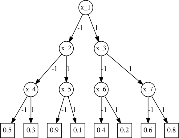
Conditional independence (and related factorizations) is not the only type of structure that can be exploited to achieve compactness. For example, consider the weighted decision tree in Figure 1. No two variables in the probability distribution in Figure 1 are independent of each other. The probability distribution cannot be represented by the product of simpler terms of disjoint domains and hence we cannot take advantage of independencies. The full probability table needs entries to be represented exactly. Nevertheless, this table can be described exactly by 8 simple decision rules, each corresponding to a path from the root to a leaf in the tree.
In this paper, we explore a novel way to exploit compact representations of high-dimensional probability tables in (approximate) probabilistic inference algorithms. Our approach is based on a (discrete) Fourier representation of the tables, which can be interpreted as a change of basis. Crucially, tables that are dense in the canonical basis can have a sparse Fourier representation. In particular, under certain conditions, probability tables can be represented (or well approximated) using a small number of Fourier coefficients. The Fourier representation has found numerous recent applications, including modeling stochastic processes (Rogers, 2000; Abbring & Salimans, 2012), manifolds (Cohen & Welling, 2015), and permutations (Huang et al., 2009). Our approach is based on Fourier representation on Boolean functions, which has found tremendous success in PAC learning (O’Donnell, 2008; Mansour, 1994; Blum et al., 1998; Buchman et al., 2012), but these ideas have not been fully exploited in the fields of probabilistic inference and graphical models.
In general, a factor over Boolean variables requires entries to be specified, and similarly the corresponding Fourier representation is dense in general, i.e., it has non-zero coefficients. However, a rather surprising fact which was first discovered by Linial (Linial et al., 1993) is that factors corresponding to fairly general classes of logical forms admit a compact Fourier representation. Linial discovered that formulas in Conjunctive Normal Form (CNF) and Disjunctive Normal Form (DNF) with bounded width (the number of variables in each clause) have compact Fourier representations.
In this paper, we introduce a novel approach for using approximate Fourier representations in the field of probabilistic inference. We generalize the work of Linial to the case of probability distributions (the weighted case where the entries are not necessarily 0 or 1), showing that a large class of probabilistic graphical models have compact Fourier representation. The proof extends the Hastad’s Switching Lemma (Håstad, 1987) to the weighted case. At a high level, a compact Fourier representation often means the weighted probabilistic distribution can be captured by a small set of critical decision rules. Hence, this notion is closely related to decision trees with bounded depth.
Sparse (low-degree) Fourier representations provide an entirely new way of approximating a probability distribution. We demonstrate the power of this idea by applying it to the variable elimination algorithm. Despite that it is conceptually simple, we show in Table 2 that the variable elimination algorithm with Fourier representation outperforms Minibucket, Belief Propagation and MCMC, and is competitive and even outperforms an award winning solver HAK on several categories of the UAI Inference Challenge.
2 Preliminaries
2.1 Inference in Graphical Models
We consider a Boolean graphical model over Boolean variables . We use bold typed variables to represent a vector of variables. For example, the vector of all Boolean variables is written as . We also use to represent the image of vector projected onto a subset of variables: where . A probabilistic graphical model is defined as:
where each is called a factor, and is a function that depends on a subset of variables whose indices are in . is the normalization factor, and is often called the partition function. In this paper, we will use and to represent and . We consider two key probabilistic inference tasks: the computation of the partition function (PR) and marginal probabilities (Marginal), in which means that is consistent with the evidence .
The Variable Elimination Algorithm is an exact algorithm to compute marginals and the partition function for general graphical models. It starts with a variable ordering . In each iteration, it eliminates one variable by multiplying all factors involving that variable, and then summing that variable out. When all variables are eliminated, the factor remaining is a singleton, whose value corresponds to the partition function. The complexity of the VE algorithm depends on the size of the largest factors generated during the elimination process, and is known to be exponential in the tree-width (Gogate & Dechter, 2004).
Detcher proposed the Mini-bucket Elimination Algorithm (Dechter, 1997), which dynamically decomposes and approximates factors (when the domain of a product exceeds a threshold) with the product of smaller factors during the elimination process. Mini-bucket can provide upper and lower bounds on the partition function. The authors of (van Rooij et al., 2009; Smith & Gogate, 2013) develop fast operations similar to the Fast Fourier transformation, and use it to speed up the exact inference. Their approaches do not approximate the probability distribution, which is a key difference from this paper.
2.2 Hadamard-Fourier Transformation
Hadamard-Fourier transformation has attracted a lot of attention in PAC Learning Theory. Table 1 provides an example where a function is transformed into its Fourier representation. The transformation works by writing using interpolation, then re-arranging the terms to get a canonical term. The example can be generalized, and it can be shown that any function defined on a Boolean hypercube has an equivalent Fourier representation.
Theorem 1.
(Hadamard-Fourier Transformation) Every can be uniquely expressed as a multilinear polynomial,
where each . This polynomial is referred to as the Hadamard-Fourier expansion of .
Here, is the power set of . Following standard notation, we will write to denote the coefficient and for the basis function . As a special case, . Notice these basis functions are parity functions. We also call a degree- coefficient of iff . In our example in Table 1, the coefficient for basis function is , which is a degree-2 coefficient.
We re-iterate some classical results on Fourier expansion. First, as with the classical (inverse) Fast Fourier Transformation (FFT) in the continuous domain, there are similar divide-and-conquer algorithms ( and ) which connect the table representation of (e.g., upper left table, Table 1) with its Fourier representation (e.g., bottom representation, Table 1). Both and run in time for a function involving variables. In fact, the length vector of all function values and the length vector of Fourier coefficients are connected by a -by- matrix , which is often called the -th Hadamard-Fourier matrix. In addition, we have the Parseval’s identity for Boolean Functions as well: .
| -1 | -1 | |
| -1 | 1 | |
| 1 | -1 | |
| 1 | 1 |
3 Low Degree Concentration of Fourier Coefficients
Fourier expansion replaces the table representation of a weighted function with its Fourier coefficients. For a function with Boolean variables, the complete table representation requires entries, and so does the full Fourier expansion. Interestingly, many natural functions can be approximated well with only a few Fourier coefficients. This raises a natural question: what type of functions can be well approximated with a compact Fourier expansion?
We first discuss which functions can be represented exactly in the Fourier domain with coefficients up to degree . To answer this question, we show a tight connection between Fourier representations with bounded degree and decision trees with bounded depth. A decision tree for a weighted function is a tree in which each inner node is labelled with one variable, and has two out-going edges, one labelled with , and other one with . The leaf nodes are labelled with real values. When evaluating the value on an input , we start from the root node, and follow the corresponding out-going edges by inspecting the value of one variable at each step, until we reach one of the leaf nodes. The value at the leaf node is the output for . The depth of the decision tree is defined as the longest path from the root node to one of the leaf nodes. Figure 1 provides a decision tree representation for a weighted Boolean function. One classical result (O’Donnell, 2008) states that if a function can be captured by a decision tree with depth , then it can be represented with Fourier coefficients up to degree :
Theorem 2.
Suppose can be represented by a decision tree of depth , then all the coefficients whose degree are larger than is zero in ’s Fourier expansion: for all such that .
We can also provide the converse of Theorem 2:
Theorem 3.
Suppose can be represented by a Fourier expansion with non-zero coefficients up to degree , then can be represented by the sum of several decision trees, each of which has depth at most .
Theorem 2 and Theorem 3 provide a tight connection between the Fourier expansion and the decision trees. This is also part of the reason why the Fourier representation is a powerful tool in PAC learning. Notice that the Fourier representation complements the classical way of approximating weighted functions exploiting independencies. To see this, suppose there is a decision tree of the same structure as in Figure 1, but has depth . According to Theorem 2, it can be represented exactly with Fourier coefficients up to degree . In this specific example, the number of non-zero Fourier coefficients is . Nonetheless, no two variables in figure 1 are independent with each other. Therefore, it’s not possible to decompose this factor into a product of smaller factors with disjoint domains (exploiting independencies). Notice that the full table representation of this factor has entries, because different nodes in the decision tree have different variables and there are variables in total in this example.
If we are willing to accept an approximate representation, low degree Fourier coefficients can capture an even wider class of functions. We follow the standard notion of -concentration:
Definition 1.
The Fourier spectrum of is -concentrated on degree up to if and only if .
We say a CNF (DNF) formula has bounded width if and only if every clause (term) of the CNF (DNF) has at most literals. In the literatures outside of PAC Learning, this is also referred to as a CNF (DNF) with clause (term) length . Linial (Linial et al., 1993) proved the following result:
Theorem 4 (Linial).
Suppose is computable by a DNF (or CNF) of width , then ’s Fourier spectrum is -concentrated on degree up to .
Linial’s result demonstrates the power of Fourier representations, since bounded width CNF’s (or DNF’s) include a very rich class of functions. Interestingly, the bound does not depend on the number of clauses, even though the clause-variable ratio is believed to characterize the hardness of satisfiability problems.
As a contribution of this paper, we extend Linial’s results to a class of weighted probabilistic graphical models, which are contractive with gap and have bounded width . To our knowledge, this extension from the deterministic case to the probabilistic case is novel.
Definition 2.
Suppose is a weighted function, we say has bounded width iff the number of variables in the domain of is no more than . We say is contractive with gap if and only if (1) for all , ; (2) ; (3) if , then .
The first and second conditions are mild restrictions. For a graphical model, we can always rescale each factor properly to ensure its range is within and the largest element is 1. The approximation bound we are going to prove depends on the gap . Ideally, we want to be small. The class of contractive functions with gap still captures a wide class of interesting graphical models. For example, it captures Markov Logic Networks (Richardson & Domingos, 2006), when the weight of each clause is large. Notice that this is one of the possible necessary conditions we found success in proving the weight concentration result. In practice, because compact Fourier representation is more about the structure of the weighted distribution (captured by a series of decision trees of given depth), graphical models with large could also have concentrated weights. The main theorem we are going to prove is as follows:
Theorem 5.
(Main) Suppose , in which every is a contractive function with width and gap , then ’s Fourier spectrum is -concentrated on degree up to when and when .
The proof of theorem 5 relies on the notion of random restriction and our own extension to the Hastad’s Switching Lemma (Håstad, 1987).
Definition 3.
Let and be subset of all the variables . Let be an assignment to remaining variables . Define to be the restricted function of on by setting all the remaining variables in according to .
Definition 4.
(-random restriction) A -random restriction of is defined as , when elements in are selected randomly with probability , and is formed by randomly setting variables in to either or . We also say is a -random restriction set.
With these definitions, we proved our weighted extension to the Hastad’s Switching Lemma:
Lemma 1.
(Weighted Hastad’s Switching Lemma) Suppose , in which every is a contractive function with width and gap . Suppose is a -random restriction set, then
in which if or if and means .
The formal proof of Lemma 1 is based on a clever generalization of the proof by Razborov for the unweighted case (Razborov, 1995), and is deferred to the supplementary materials.
Lemma 2.
Suppose and . is a -random restriction set. , and let decision tree with depth such that , then the Fourier spectrum of is -concentrated on degree up to .
Proof.
We first bound . With probability , there is a decision tree with depth such that . In this scenario,
| (1) |
This is because due to Theorem 2, for all such that . Because for all , hence the right side of Equation 1 must satisfy
| (2) |
The second to the last equality of Equation 2 is due to the Parseval’s Identity. With probability , there are no decision trees close to . However, because , we must have . Summarizing these two points, we have:
Using a known result , we have:
| (3) |
The distribution of random variable is Binomial(). When , this variable has mean at least , using Chernoff bound, . Therefore,
We get our claim . ∎
Now we are ready to prove Theorem 5. Firstly suppose , choose , which ensures . Next choose , , which ensures
Choose large enough, such that . Now we have . At the same time, .111 corresponds to the classical CNF (or DNF) case.
4 Variable Elimination in the Fourier Domain
We have seen above that a Fourier representation can provide a useful compact representation of certain complex probability distributions. In particular, this is the case for distributions that can be captured with a relatively sparse set of Fourier coefficients. We will now show the practical impact of this new representation by using it in an inference setting. In this section, we propose an inference algorithm which works like the classic Variable Elimination (VE) Algorithm, except for passing messages represented in the Fourier domain.
The classical VE algorithm consists of two basic steps – the multiplication step and the elimination step. The multiplication step takes and , and returns , while the elimination step sums out one variable from by returning . Hence, the success of the VE procedure in the Fourier domain depends on efficient algorithms to carry out the aforementioned two steps. A naive approach is to transform the representation back to the value domain, carry out the two steps there, then transform it back to Fourier space. While correct, this strategy would eliminate all the benefits of Fourier representations.
Luckily, the elimination step can be carried out in the Fourier domain as follows:
Theorem 6.
Suppose has a Fourier expansion: . Then the Fourier expansion for when is summed out is: , where if and if .
The proof is left to the supplementary materials. From Theorem 6, one only needs a linear scan of all the Fourier coefficients of in order to compute the Fourier expansion for . Suppose has non-zero coefficients in its Fourier representation, this linear scan takes time .
There are several ways to implement the multiplication step. The first option is to use the school book multiplication. To multiply functions and , one multiplies every pair of their Fourier coefficients, and then combines similar terms. If and have and terms in their Fourier representations respectively, this operation takes time . As a second option for multiplication, one can convert and to their value domain, multiply corresponding entries, and then convert the result back to the Fourier domain. Suppose the union of the domains of and has variables ( Fourier terms), the conversion between the two domains dominates the complexity, which is . Nonetheless, when and are relatively dense, this method could have a better time complexity than the school book multiplication. In our implementation, we trade the complexity between the aforementioned two options, and always use the one with lower time complexity.
Because we are working on models in which exact inference is intractable, sometimes we need to truncate the Fourier representation to prevent an exponential explosion. We implement two variants for truncation. One is to keep low degree Fourier coefficients, which is inspired by our theoretical observations. The other one is to keep Fourier coefficients with large absolute values, which offers us a little bit extra flexibility, especially when the whole graphical model is dominated by a few key variables and we would like to go over the degree limitations occasionally. We found both variants work equally well.
5 Experiments
5.1 Weight Concentration on Low Degree Coefficients
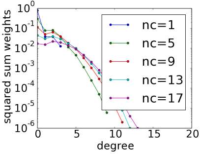
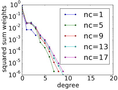
We first validate our theoretical results on the weight concentration on low-degree coefficients in Fourier representations. We evaluate our results on random weighted 3-SAT instances with 20 variables. Small instances are chosen because we have to compute the full Fourier spectrum. The weighted 3-SAT instances is specified by a CNF and a weight . Each factor corresponds to a clause in the CNF. When the clause is satisfied, the corresponding factor evaluates to 1, otherwise evaluates to . For each and the number of clauses , we randomly generate 100 instances. For each instance, we compute the squared sum weight at each degree: . Figure 2 shows the median value of the squared sum weight over 100 instances for given and in log scale. As seen from the figure, although the full representation involves coefficients up to degree 20 (20 variables), the weights are concentrated on low degree coefficients (up to 5), regardless of , which is in line with the theoretical result.
5.2 Applying Fourier Representation in Variable Elimination
| Category | #ins | Minibucket | Fourier (max coef) | Fourier (min deg) | BP | MCMC | HAK |
|---|---|---|---|---|---|---|---|
| bn2o-30-* | 18 | 3.91 | 0.34 | ||||
| grids2/50-* | 72 | 5.12 | – | ||||
| grids2/75-* | 103 | 18.34 | – | ||||
| grids2/90-* | 105 | 26.16 | – | ||||
| blockmap_05* | 48 | 0.11 | – | ||||
| students_03* | 16 | 2.20 | – | ||||
| mastermind_03* | 48 | 7.83 | 0.47 | 0.36 | 27.69 | – | |
| mastermind_04* | 32 | 12.30 | 20.59 | – | |||
| mastermind_05* | 16 | 4.06 | 22.47 | – | |||
| mastermind_06* | 16 | 22.34 | 17.18 | – | |||
| mastermind_10* | 16 | 275.82 | 5.63 | 2.98 | 26.32 | – |
We integrate the Fourier representation into the variable elimination algorithm, and evaluate its performance as an approximate probabilistic inference scheme to estimate the partition function of undirected graphical models. We implemented two versions of the Fourier Variable Elimination Algorithm. One version always keeps coefficients with the largest absolute values when we truncate the representation. The other version keeps coefficients with the lowest degree. Our main comparison is against Mini-Bucket Elimination, since the two algorithms are both based on variable elimination, with the only difference being the way in which the messages are approximated. We obtained the source code from the author of Mini-Bucket Elimination, which includes sophisticated heuristics for splitting factors. The versions we obtained are used for Maximum A Posteriori Estimation (MAP). We augment this version to compute the partition function by replacing the maximization operators by summation operators. We also compare our VE algorithm with MCMC and Loopy Belief Propagation. We implemented the classical Ogata-Tanemura scheme (Ogata & Tanemura, 1981) with Gibbs transitions in MCMC to estimate the partition function. We use the implementation in LibDAI (Mooij, 2010) for belief propagation, with random updates, damping rate of 0.1 and the maximal number of iterations 1,000,000. Throughout the experiment, we control the number of MCMC steps, the -bound of Minibucket and the message size of Fourier VE to make sure that the algorithms complete in reasonable time (several minutes).
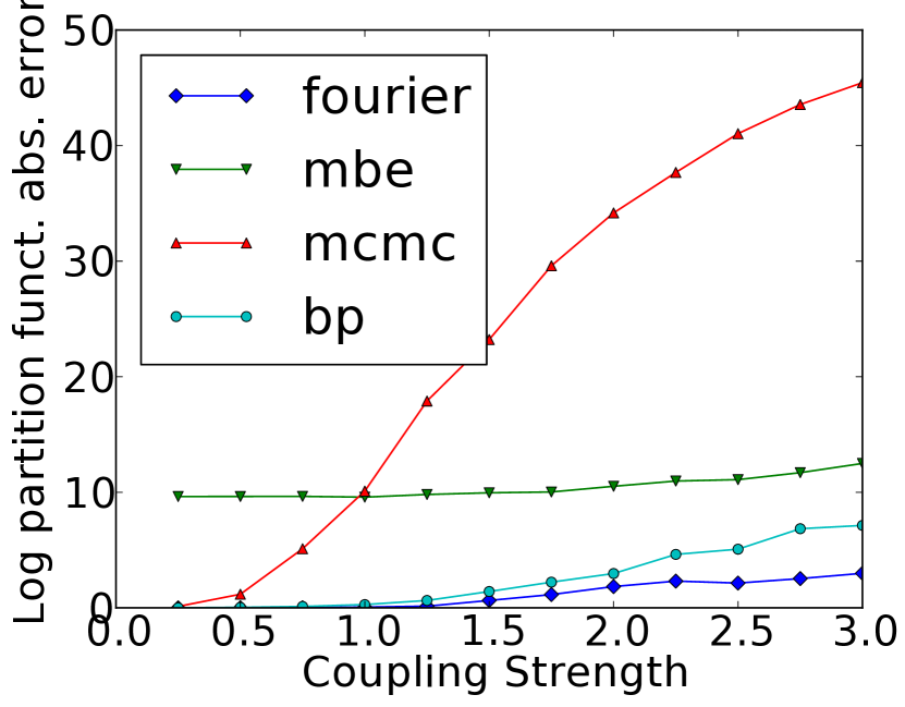
We first compare on small instances for which we can compute ground truth using the state-of-the-art exact inference algorithm ACE (Darwiche & Marquis, 2002). We run on 15-by-15 Ising models with mixed coupling strengths and various field strengths. We run 20 instances for each coupling strength. For a fair comparison, we fix the size of the messages for both Fourier VE and Mini-bucket to . Under this message size VE algorithms cannot handle the instances exactly. Figure 3 shows the results. The performance of the two versions of the Fourier VE algorithm are almost the same, so we only show one curve. Clearly the Fourier VE Algorithm outperforms the MCMC and the Mini-bucket Elimination. It also outperforms Belief Propagation when the field strength is relatively strong.
In addition, we compare our inference algorithms on large benchmarks from the UAI 2010 Approximate Inference Challenge (UAI, ). Because we need the ground truth to compare with, we only consider benchmarks that can be solved by ACE (Darwiche & Marquis, 2002) in 2 hours time, and 8GB of memory. The second column of Table 2 shows the number of instances that ACE completes with the exact answer. The 3rd to the 7th column of Table 2 shows the result for several inference algorithms, including the Minibucket algorithm with -bound of 20, two versions of the Fourier Variable Elimination algorithms, belief propagation and MCMC. To be fair with Minibucket, we set the message size for Fourier VE to be 1,048,576 (). Because the complexity of the multiplication step in Fourier VE is quadratic in the number of coefficients, we further shrink the message size to 1,024 () during multiplication. We allow 1,000,000 steps for burn in and another 1,000,000 steps for sampling in the MCMC approach. The same with the inference challenge, we compare inference algorithms on the difference in the log partition function . The table reports the median differences, which are averaged over all benchmarks in each category. If one algorithm fails to complete on one instance, we count the difference in partition function as , so it is counted as the worst case when computing the median. For MCMC, “–” means that the Ogata-Tanemura scheme did not find a belief state with substantial probability mass, so the result is way off when taking the logarithm. The results in Table 2 show that Fourier Variable Elimination algorithms outperform MCMC, BP and Minibucket on many categories in the Inference challenge. In particular, Fourier VE works well on grid and structural instances. We also listed the performance of a Double-loop Generalized Belief Propagation (Heskes et al., 2003) in the last column of Table 2. This implementation won one category in the Inference challenge, and contains various improvements besides the techniques presented in the paper. We used the parameter settings for high precision in the Inference challenge for HAK. As we can see, Fourier VE matches or outperforms this implementation in some categories. Unlike fully optimized HAK, Fourier VE is a simple variable elimination algorithm, which involves passing messages only once. Indeed, the median time for Fourier VE to complete on bn2o instances is about 40 seconds, while HAK takes 1800 seconds. We are researching on incorporating the Fourier representation into message passing algorithms.
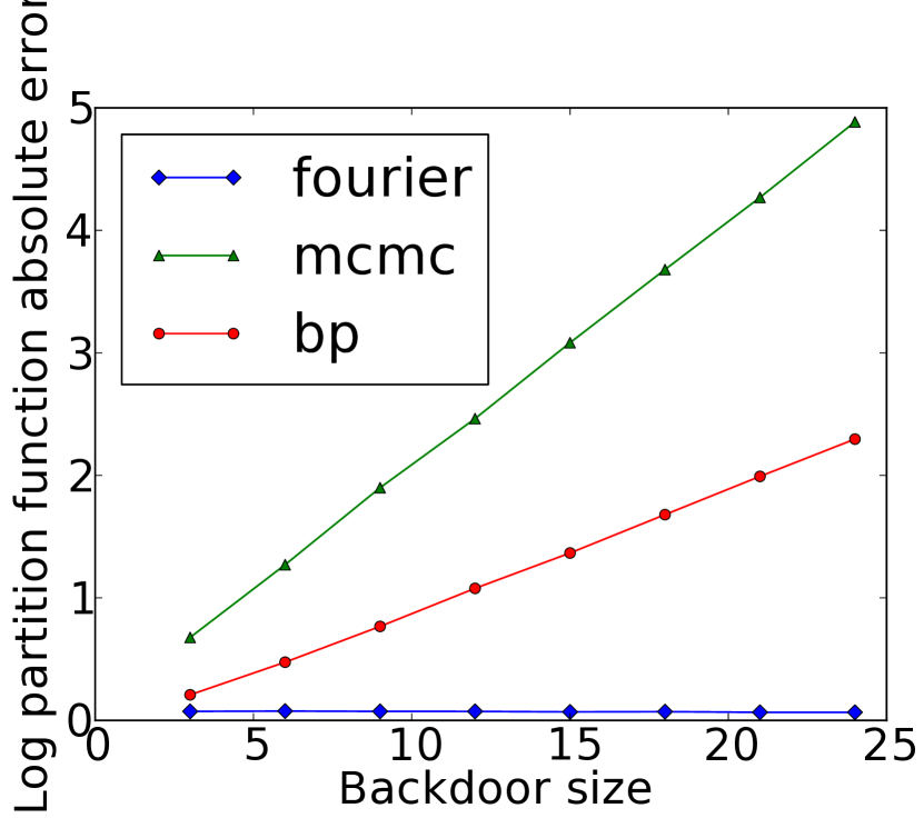
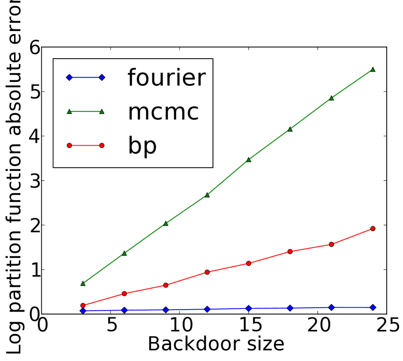
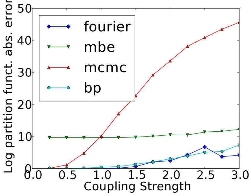
Next we evaluate their performance on a synthetically generated benchmark beyond the capability of exact inference algorithms. For one instance of this benchmark, we randomly generate factors of size with low coupling weights. We then add a backdoor structure to each instance, by enforcing coupling factors of size in which the variables of the factor must take the same value. For these instances, we can compute the expected value of the partition function and compare it with the output of the algorithms. We report the results on Figure 4. Here the experimental setup for each inference algorithm is kept the same as the previous algorithm. The Mini-bucket approach is not reported, as it performs very poorly on these instances. The performance of the two implementations of Fourier VE are again similar, so they are combined into one curve. These results show that the Fourier approach outperforms both MCMC and Belief Propagation, and suggest that it can perform arbitrarily better than both approaches as the size of the backdoor increases.
Finally, we compare different inference algorithms on a machine learning application. Here we learn a grid Ising model from data. The computation of the partition function is beyond any exact inference methods. Hence in order to compare the performance of different inference algorithms, we have to control the training data that are fit into the Ising Model, to be able to predict what the learned model looks like. To generate training pictures, we start with a template with nine boxes (shown in Figure 5(a)). The training pictures are of size , so the partition function cannot be computed exactly by variable elimination algorithms with message size . Each of the nine boxes in the template will have a 50% opportunity to appear in a training picture, and the occurrences of the nine boxes are independent of each other. We further blur the training images with 5% white noise. Figures 5(b) and 5(c) show two examples of the generated training images. We then use these training images to learn a grid Ising Model:
where , are the node and edge set of a grid, respectively. We train the model using contrastive divergence (Hinton, 2002), with steps of blocked Gibbs updates, on such training images. (As we will see, vanilla Gibbs sampling, which updates one pixel at a time, does not work well on this problem.) We further encourage a sparse model by using a L1 regularizer.


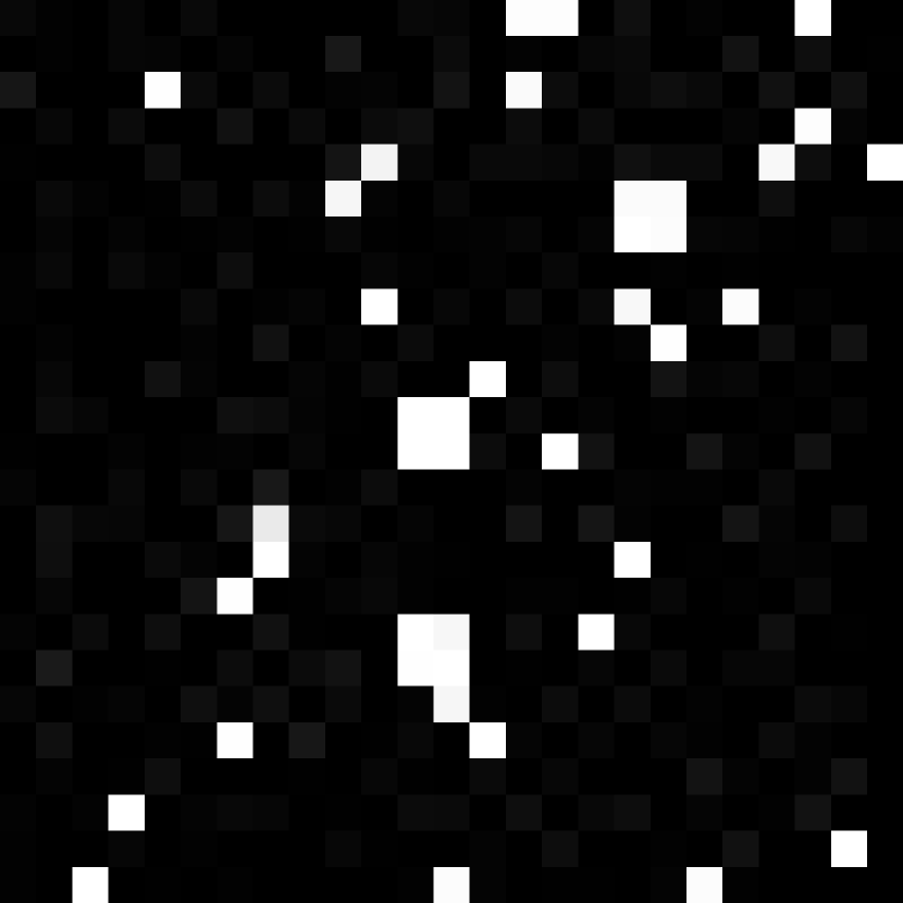


Once the model is learned, we use inference algorithms to compute the marginal probability of each pixel. Figure 5(d) 5(e) 5(f) and 5(g) show the marginals computed for the Fourier VE, MCMC, Minibucket Elimination, and the Mean Field on the learned model (white means the probability is close to 1, black means close to 0). Both the Minibucket and the Fourier VE keep a message size of , so they cannot compute the marginals exactly. Fourier VE keeps coefficients with largest absolute value during multiplication. For pixels outside of the nine boxes, in most circumstances they are black in the training images. Therefore, their marginals in the learned model should be close to 0. For pixels within the nine boxes, half of the time they are white in the training images. Hence, the marginal probabilities of these pixels in the learned model should be roughly 0.5. We validated the two aforementioned empirical observations on images with small size which we can compute the marginals exactly. As we can see, only the Fourier Variable Elimination Algorithm is able to predict a marginal close to 0.5 on these pixels. The performance of the MCMC algorithm (a Gibbs sampler, updating one pixel at a time) is poor. The Minibucket Algorithm has noise on some pixels. The marginals of the nine boxes predicted by mean field are close to 1, a clearly wrong answer.
6 Conclusion
We explore a novel way to exploit compact representations of high-dimensional probability distributions in approximate probabilistic inference. Our approach is based on discrete Fourier Representation of weighted Boolean Functions, complementing the classical method of exploiting conditional independence between the variables. We show that a large class of weighted probabilistic graphical models have a compact Fourier representation. This theoretical result opens up a novel way of approximating probability distributions. We demonstrate the significance of this approach by applying it to the variable elimination algorithm, obtaining very encouraging results.
Acknowledgments
This research was supported by National Science Foundation (Award Number 0832782, 1522054, 1059284).
References
- (1) Uai 2010 approximate inference challenge. http://www.cs.huji.ac.il/project/UAI10.
- Abbring & Salimans (2012) Abbring, Jaap H and Salimans, Tim. The likelihood of mixed hitting times. Technical report, working paper, 2012. URL http://portal.uni-freiburg.de/empiwifo/sonstige-dateien/abbring.pdf.
- Bahar et al. (1993) Bahar, R.I., Frohm, E.A., Gaona, C.M., Hachtel, G.D., Macii, E., Pardo, A., and Somenzi, F. Algebraic decision diagrams and their applications. In Computer-Aided Design, 1993.
- Blum et al. (1998) Blum, Avirim, Burch, Carl, and Langford, John. On Learning Monotone Boolean Functions. In FOCS, pp. 408–415, 1998.
- Buchman et al. (2012) Buchman, David, Schmidt, Mark W., Mohamed, Shakir, Poole, David, and de Freitas, Nando. On sparse, spectral and other parameterizations of binary probabilistic models. In AISTATS, 2012.
- Cohen & Welling (2015) Cohen, Taco and Welling, Max. Harmonic exponential families on manifolds. In Proceedings of the 32nd International Conference on Machine Learning, ICML, 2015.
- Darwiche & Marquis (2002) Darwiche, Adnan and Marquis, Pierre. A knowledge compilation map. J. Artif. Int. Res., 2002.
- Dechter (1997) Dechter, Rina. Mini-buckets: A general scheme for generating approximations in automated reasoning. In Proceedings of the Fifteenth International Joint Conference on Artificial Intelligence, 1997.
- Flerova et al. (2011) Flerova, Natalia, Ihler, Er, Dechter, Rina, and Otten, Lars. Mini-bucket elimination with moment matching. In In NIPS Workshop DISCML, 2011.
- Friesen & Domingos (2015) Friesen, Abram L. and Domingos, Pedro. Recursive decomposition for nonconvex optimization. In Proceedings of the 24th International Joint Conference on Artificial Intelligence, 2015.
- Gogate & Dechter (2004) Gogate, Vibhav and Dechter, Rina. A complete anytime algorithm for treewidth. In Proceedings of the 20th Conference on Uncertainty in Artificial Intelligence, 2004.
- Gogate & Domingos (2013) Gogate, Vibhav and Domingos, Pedro M. Structured message passing. In UAI, 2013.
- Håstad (1987) Håstad, Johan. Computational Limitations of Small-depth Circuits. MIT Press, Cambridge, MA, USA, 1987. ISBN 0262081679.
- Hazan & Jaakkola (2012) Hazan, Tamir and Jaakkola, Tommi S. On the partition function and random maximum a-posteriori perturbations. In ICML, 2012.
- Heskes et al. (2003) Heskes, Tom, Albers, Kees, and Kappen, Bert. Approximate inference and constrained optimization. In Proceedings of the Nineteenth Conference on Uncertainty in Artificial Intelligence, UAI’03, 2003.
- Hinton (2002) Hinton, Geoffrey E. Training products of experts by minimizing contrastive divergence. Neural Comput., pp. 1771–1800, 2002.
- Huang et al. (2009) Huang, Jonathan, Guestrin, Carlos, and Guibas, Leonidas J. Fourier theoretic probabilistic inference over permutations. Journal of Machine Learning Research, 10:997–1070, 2009.
- Ihler et al. (2012) Ihler, Alexander T., Flerova, Natalia, Dechter, Rina, and Otten, Lars. Join-graph based cost-shifting schemes. In UAI, 2012.
- Jordan et al. (1999) Jordan, Michael I., Ghahramani, Zoubin, Jaakkola, Tommi S., and Saul, Lawrence K. An introduction to variational methods for graphical models. Mach. Learn., 1999.
- Linden et al. (2003) Linden, Greg, Smith, Brent, and York, Jeremy. Amazon.com recommendations: Item-to-item collaborative filtering. IEEE Internet Computing, 2003.
- Linial et al. (1993) Linial, Nathan, Mansour, Yishay, and Nisan, Noam. Constant depth circuits, fourier transform, and learnability. J. ACM, 40(3), 1993.
- Mansour (1994) Mansour, Yishay. Learning Boolean functions via the Fourier transform. advances in neural computation and learning, 0:1–28, 1994. URL http://link.springer.com/chapter/10.1007/978-1-4615-2696-4_11.
- Mateescu et al. (2010) Mateescu, Robert, Kask, Kalev, Gogate, Vibhav, and Dechter, Rina. Join-graph propagation algorithms. J. Artif. Intell. Res. (JAIR), 37, 2010.
- Mooij (2010) Mooij, Joris M. libDAI: A free and open source C++ library for discrete approximate inference in graphical models. Journal of Machine Learning Research, 11:2169–2173, August 2010. URL http://www.jmlr.org/papers/volume11/mooij10a/mooij10a.pdf.
- O’Donnell (2008) O’Donnell, Ryan. Some topics in analysis of boolean functions. Proceedings of the fourtieth annual ACM symposium on Theory of computing - STOC 08, pp. 569, 2008. doi: 10.1145/1374376.1374458. URL http://dl.acm.org/citation.cfm?doid=1374376.1374458.
- Ogata & Tanemura (1981) Ogata, Yosihiko and Tanemura, Masaharu. Estimation of interaction potentials of spatial point patterns through the maximum likelihood procedure. Annals of the Institute of Statistical Mathematics, 1981. ISSN 0020-3157.
- Razborov (1995) Razborov, Alexander A. Bounded arithmetic and lower bounds in boolean complexity. In Feasible Mathematics II, Progress in Computer Science and Applied Logic. 1995. ISBN 978-1-4612-7582-4.
- Richardson & Domingos (2006) Richardson, Matthew and Domingos, Pedro. Markov logic networks. Mach. Learn., 2006.
- Rogers (2000) Rogers, L Chris G. Evaluating first-passage probabilities for spectrally one-sided lévy processes. Journal of Applied Probability, pp. 1173–1180, 2000.
- Smith & Gogate (2013) Smith, David and Gogate, Vibhav. The inclusion-exclusion rule and its application to the junction tree algorithm. In Proceedings of the Twenty-Third International Joint Conference on Artificial Intelligence, 2013.
- Sontag et al. (2008) Sontag, David, Meltzer, Talya, Globerson, Amir, Jaakkola, Tommi, and Weiss, Yair. Tightening lp relaxations for map using message passing. In UAI, pp. 503–510, 2008.
- van Rooij et al. (2009) van Rooij, Johan M. M., Bodlaender, Hans L., and Rossmanith, Peter. Dynamic programming on tree decompositions using generalised fast subset convolution. In Algorithms - ESA, 17th Annual European Symposium, 2009.
- Wainwright et al. (2003) Wainwright, Martin J., Jaakkola, Tommi S., and Willsky, Alan S. Tree-reweighted belief propagation algorithms and approximate ML estimation by pseudo-moment matching. In Proceedings of the Ninth International Workshop on Artificial Intelligence and Statistics, 2003.
Supplementary Materials
Proof of Lemma 1
Let be the collection of restrictions on Boolean variables . Each restriction in leaves a set of variables open, while it fixes all other variables to either -1 or 1. It is easy to see that the size of is given by:
| (4) |
For a restriction , call bad if and only if for all decision tree with depth , there exists at least one input , such that . Let be the set of all bad restrictions, ie: . To prove the lemma, it is sufficient to prove that
| (5) |
In the proof that follows, for every bad restriction , we establish a bijection between and , in which is a restriction in and is a certificate from a witness set . In this case, the number of distinct ’s is bounded by the number of pairs:
| (6) |
For a restriction , we form the canonical decision tree for under precision as follows:
-
1.
We start with a fixed order for the variables and another fixed order for the factors.
-
2.
If is a constant function, or , stop.
-
3.
Otherwise, under restriction , some factors evaluate to fixed values (all variables in these factors are fixed or there are free variables, but all assignments to these free variables lead to value 1), while other factors do not. Examine the factors according to the fixed factor order until reaching the first factor that still does not evaluate to a fixed value.
-
4.
Expand the open variables of this factor, under the fixed variable order specified in step 1. The result will be a tree (The root branch is for the first open variable. The branches in the next level is for the second open variable, etc).
-
5.
Each leaf of this tree corresponds to , in which is a value restriction for all open variables of the factor. Recursively apply step 2 to 5 for function , until the condition in step 2 holds. Then attach the resulting tree to this leaf.
Figure 6 provides a graphical demonstration of a canonical decision tree.
Now suppose restriction is bad. By definition, for any decision tree of depth , there exists at least one input , such that . The canonical decision tree is no exception. Therefore, there must be a path in the canonical decision tree of , which has more than variables. Furthermore, these variables can be split into () segments, each of which corresponds to one factor. Let () be these factors, and let be the assignments of the free variables for in path . Now for each factor , by the definition of the canonical decision tree, under the restriction , must have a branch whose value is no greater than (otherwise all evaluates to 1). We call this branch the “compressing” branch for factor . Let the variable assignment which leads to this compressing branch for be . Let . Then we map the bad restriction to and an auxiliary advice string that we are going to describe.
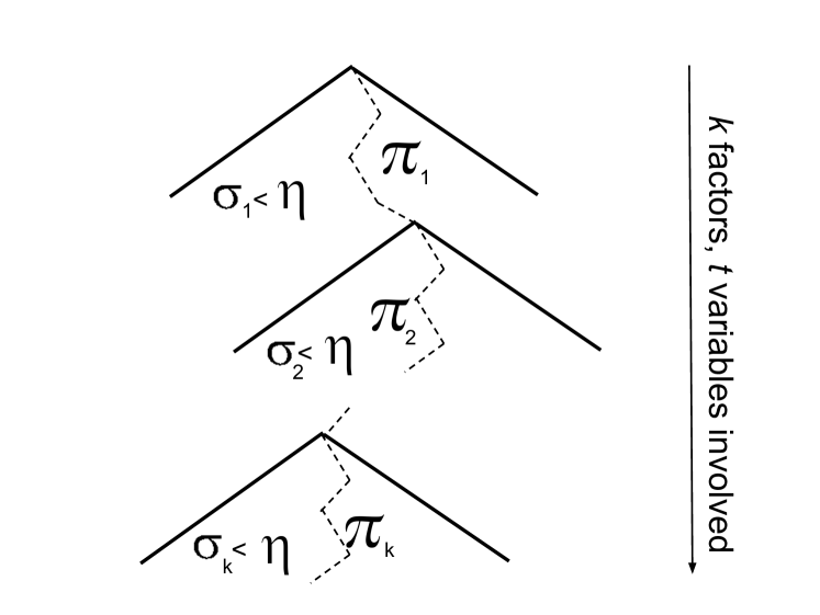
It is self-explanatory that we can map from any bad restriction to . The auxiliary advice is used to establish the backward mapping, i.e. the mapping from to . When we look at the result of , we will notice that at least one factor is set to its compressing branch (because we set to its compressing branch in the forward mapping). Now there could be other factors set at their compressing branches (because of ), but an important observation is that: the number of factors at their compressing branches cannot exceed , because otherwise, the other factors already render , and the canonical decision tree should have stopped on expanding this branch. We therefore could record the index number of out of all the factors that are fixed at their compressing branches in the auxiliary advice string, so we can find in the backward mapping. Notice that this index number will be between 1 and , so it takes bits to store it.
Now with the auxiliary information, we can identify which factor is . The next task is to identify which variables in are fixed by , and which are fixed by . Moreover, if one variable is fixed by , we would like to know its correct values in . To do this, we introduce additional auxiliary information: for each factor , suppose it has free variables under restriction , we use integers to mark the indices of these free variables. Because each is of width at most , every integer of this type is between 1 and (therefore can be stored in bits). Also, it requires integers of this type in total to keep this information, because we have free variables in total for .
Notice that it is not sufficient to keep these integers. We further need separators, which tell which integer belongs to which factor . Aligning these integers in a line, we need separators to break the line into segments. These separators can be represented by bits, in which the -th bit is 1 if and only if there is a separator between the -th and (+1)-th integer (we have integers at most). With these two pieces of information, we are able to know the locations of free variables set by for each factor .
We further need to know the values for each variable in . Therefore, we add in another -bit string, each bit is either 0 or 1. 0 means the assignment of the corresponding variable in is the same as the one in , 1 means the opposite.
With all this auxiliary information, we can start from , find the first factor , further identify which variables are set by in , and set back its values in . Then we start with , we can find in the same process, and continue. Finally, we will find all variables in and back up the original restriction .
Now to count the length of the auxiliary information, the total length is bits. Therefore, we can have a one-to-one mapping between elements in and , in which the size of is bounded by .
In all,
| (7) | ||||
| (8) | ||||
| (9) | ||||
| (10) |
Proof of Theorem 3
For each term in the Fourier expansion whose degree is less than or equal to , we can treat this term as a weighted function involving less than or equal to variables. Therefore, it can be represented by a decision tree, in which each path of the tree involves no more than variables (therefore the tree is at most at the depth of ). Because is represented as the sum over a set of Fourier terms up to degree , it can be also represented as the sum of the corresponding decision trees.
Proof of Theorem 6
Let the Fourier expansion of be: , we have: