Peak-Aware Online Economic Dispatching for Microgrids

Abstract

By employing local renewable energy sources and power generation units while connected to the central grid, microgrid can usher in great benefits in terms of cost efficiency, power reliability, and environmental awareness. Economic dispatching is a central problem in microgrid operation, which aims at effectively scheduling various energy sources to minimize the operating cost while satisfying the electricity demand. Designing intelligent economic dispatching strategies for microgrids, however, is drastically different from that for conventional central grids, due to two unique challenges. First, the erratic renewable energy emphasizes the need for online algorithms. Second, the widely-adopted peak-based pricing scheme brings out the need for new peak-aware strategy design. In this paper, we tackle these critical challenges and devise peak-aware online economic dispatching algorithms. For microgrids with fast-responding generators, we prove that our deterministic and randomized algorithms achieve the best possible competitive ratios $2-\beta$ and $e/(e-1+\beta)$, respectively, where $\beta\in[0,1]$ is the ratio between the minimum grid spot price and the local-generation price. Our results characterize the fundamental price of uncertainty of the problem. For microgrids with slow-responding generators, we first show that a large competitive ratio is inevitable. Then we leverage limited prediction of electricity demand and renewable generation to improve the competitiveness of the algorithms. By extensive empirical evaluations using real-world traces, we show that our online algorithms achieve near offline-optimal performance. In a representative scenario, our algorithm achieves $23\%$ and $11\%$ cost reduction as compared to the case without local generation units and the case using peak-oblivious algorithms, respectively.

1 Introduction

Microgrid represents a promising paradigm of future electric power systems that autonomously coordinate distributed renewable energy source (e.g., solar PVs), local generation unit (e.g., gas generators), and the external grid to satisfy time-varying energy demand of a local community. As compared to traditional grids, microgrid has recognized advantages in cost efficiency, environmental awareness, and power reliability. Consequently, worldwide installed microgrid capacity has witnessed a phenomenon growth, reaching 866 MW in 2014, and is expected to reach 4,100 MW by 2020 [4].

Energy generation scheduling in microgrid determines the power output level of local generation units and power to be procured from external grid, with the goal of minimizing the total cost over a pre-determined billing cycle. The scheduling plan should meet the time-varying energy demand and respect physical constraints of the generation units. Such problem has been studied extensively in the power system literature for large-scale traditional grids. Two main variants are unit commitment [13] and economic dispatching [10] problems. The unit commitment problem typically optimizes the start-up and the shut-down schedule of power generation units, whereas the economic dispatching problem optimally schedules the output levels given the on/off status as the input parameters. In this paper, we focus on economic dispatching problem in microgrid scenarios.

At first glance, economic dispatching in microgrid may appear to be a small-scale version of the classical urban-wide economic dispatching problem. However, the following two unprecedented challenges make the problem fundamentally different, thereby the previous solutions inapplicable.

$\vartriangleright$ Uncontrollable, intermittent, and uncertain energy sources. Classical scheduling strategies rely on accurate prediction of future demand and dispatch-able supply [10]. In microgrids, however, the renewable sources are highly uncontrollable (not available on-demand), intermittent (irregular fluctuations), and uncertain (hard to predict accurately). Incorporating a large fraction of such renewable energy sources makes conventional strategies not applicable, and calls for new online scheduling strategies that do not rely on accurate prediction of demand and renewable generation [16, 14].

$\vartriangleright$ Peak-based charging model of the external grid. The real-world pricing scheme for consumers with large loads (such as universities or data centers) adopts a hybrid time-of-use and peak-based charging model where the electricity bill consists of both the total energy usage and the peak demand drawn over the billing cycle. The motivation is to encourage large customers to smooth their demand, thereby the utility provider can reduce its planned capacity obligations. The peak price is often more than 100 times higher than the maximum (on-peak) spot price, e.g., $118$ times for PG&E [5], and $227$ times for Duke Energy Kentucky [3] . Consequently, the contribution of peak charge in the electricity bill for a typical costumer can be considerable, e.g., from 20% to 80% for several Google data centers [21]. These observations suggest that economic dispatching strategies with peak-based charging model taken into account (referred to as peak-aware economic dispatching) may substantially reduce the total operating costs for microgrids as compared to economic dispatching strategies oblivious to peak-based charging (referred to as peak-oblivious economic dispatching). This is indeed the case as verified by our real-world trace-driven evaluation in Sec. 5.

All previous researches on microgrid economic dispatching, that we are aware of and review in Sec. 6, adopt a peak-oblivious cost model, wherein the costumer bill is computed by total energy usage following a time-of-use pricing scheme. To the best of our knowledge, this work is the first that addresses the peak-aware economic dispatching problem using competitive online algorithms in microgrid scenario. The main contributions of the paper are summarized as follows:

$\vartriangleright$ We identify and formulate the peak-aware economic dispatching problem of minimizing the operating cost for microgrids under the hybrid time-of-use and peak-based pricing scheme in Sec. 2. Notably, two aforementioned challenges change the structure of the problem fundamentally (see the discussions in Sec. 3.4 for an example) and call for different online algorithm design.

$\vartriangleright$ In Sec. 3, we focus on “fast-responding” generator scenario, where the ramping constraints (i.e., the maximum change in output level over successive steps) of local generators are inactive. We follow a divide-and-conquer approach and decompose the problem into multiple sub-problems, solve the sub-problems by their “rent-or-buy” nature, and then combine the solutions to obtain a solution for the original problem. We then demonstrate that the competitive ratios of our algorithms are $\left(2-\beta\right)$ and $e/\left(e-1+\beta\right)$ for deterministic and randomized versions respectively, where $\beta\in\left[0,1\right]$ is the ratio between the minimum grid spot price and the generator price. We prove that the ratios are the best possible. As such, these results characterize the fundamental price of uncertainty for the problem.

$\vartriangleright$ For “slow-responding” generator scenario in Sec. 4, where the ramping constraints are active, we firstly show that a large competitive ratio is inevitable without any future information. We then design an online algorithm with a small competitive ratio by taking the advantage of sufficient looking-ahead information. Our results suggest looking-head as a useful mechanism to neutralize the ramping constraints in online algorithm design.

$\vartriangleright$ In Sec. 5, by extensive evaluations using real-world traces, we show that our online algorithms can achieve satisfactory empirical performance. Furthermore, our peak-aware online algorithms achieve near offline-optimal performance, and outperform the peak-oblivious designs [16, 14] under various settings. The substantial cost reduction shows the benefit and necessity of designing peak-aware strategies for economic dispatching in microgrids.

2 Problem Formulation

In the microgrid economic dispatching problem, the objective is to orchestrate various energy sources to minimize the operating cost while satisfying the electricity demand.

We consider one billing cycle, which is a finite time horizon set ${\mathcal{T}=\{1,\dots,T\}}$ with $T$ discrete time slots. In practice, the duration of one cycle is usually one month and the length of each time slot is $15$ minutes [5]. The key notations used in this paper are defined in Table 1.

Table 1: Key notations

Notation	Definition
$T$	The total number of time slots
$\mathcal{T}$	The time slot set
$e(t)$	The net electricity demand
$u(t)$	The electricity level obtained from local generators
$v(t)$	The electricity level obtained from electricity grid
$p_{e}(t)$	The spot price of the electricity from grid at time $t,p_{e}^{\min}\leq p_{e}(t)\leq p_{e}^{\max}$, ($/KWh)
$p_{g}$	The unit cost of the electricity by local generators ($/KWh)
$p_{m}$	The peak demand price of the electricity grid ($/KWh)
$R^{\textsf{u}}$	The maximum ramping up rate of local generator
$R^{\textsf{d}}$	The maximum ramping down rate of local generator
$C$	Local generator capacity

Net electricity demand. We consider arbitrary renewable energy generation. Let $e(t)$ be the net electricity demand in time slot $t$, i.e., the total electricity demand subtracted by the renewable generation. For ease of presentation and discussion, we assume $e(t)$ only takes nonnegative integer values. Note that we do not assume any specific stochastic model of $e(t)$.

Local generation. There are local generators deployed in the microgrid with $C$ total generation capacity, i.e., they can jointly satisfy at most $C$ units of electricity demand. We consider a practical setting where the generator’s incremental power output in two consecutive slots is limited by the ramping-up and ramping-down constraints $R^{\textsf{u}}$ and $R^{\textsf{d}}$, respectively. Most microgrids today employ small-capacity generators that are powered by gas turbines or diesel engines. These generators are “fast-responding” in the sense that they have large ramping-up/-down rates. Meanwhile, there are also “slow-responding” generators with small ramping-up/-down rates. We denote $p_{g}$ as the cost of generating unit electricity using local generation.

Electricity from the external grid. The microgrid can also obtain electricity supply from the external grid for unbalanced electricity demand in an on-demand manner. We denote the spot price at time $t$ from the external grid as $p_{e}(t)$. We assume that $p_{e}(t)\geq p_{e}^{\min}\geq 0$ . Again, we do not assume any stochastic model of $p_{e}(t)$. For ease of discussion later, we define $\beta\triangleq p_{e}^{\min}/p_{g}$ as the ratio between the minimum grid price and the unit cost of local generation.

Cost model. The microgrid operating cost in $\mathcal{T}$ includes the expense of purchasing electricity from the external grid and that of local generation. Let $v(t)$ be the amount of electricity purchased from the external grid and $u(t)$ be the amount of electricity generated locally.

The cost of grid electricity consists of volume charge and peak charge. The volume charge is simply the sum of volume cost in all the time slots, i.e., $\sum_{t}p_{e}(t)v(t)$. In practice, the peak charge is based on the maximum single-slot power and the peak price unit is $/KW [5], which is different from the spot price unit $/KWh. Let the peak price in $\$/\textrm{KW}$ be $\tilde{p}_{m}$ and the length of one time slot be $\delta$ (e.g., $0.25$ hour), we convert the peak price to $/KWh as $p_{m}=\tilde{p}_{m}/\delta$. Consequently, the peak charge is $p_{m}\max_{t}v(t)$, i.e., the peak demand over the billing cycle (in KWh) multiplied by $p_{m}$ (in $/KWh). This method is similar to the one used in [21]. We remark that $p_{m}$ is usually more than 100 times larger than $p_{e}(t)$ [5].

For local generation, the cost of a generator to generate $\theta$ amount of electricity is commonly modeled as a quadratic function [13], i.e., say, $a\theta^{2}+b\theta+c$. The coefficient $a$ is usually orders of magnitude smaller than $b$ (e.g., for a typical oil generator with capacity 15MW, $a=0.007,b=48.5$) . Consequently, for small-capacity generators employed in microgrids, the quadratic term $a\theta^{2}$ is usually much smaller than the linear term $b\theta$ and is negligible. Let $p_{g}$ be the unit generating cost. The total local generation cost is simply $\sum_{t}p_{g}u(t)$. In this study, we focus on the case where $p_{g}\geq p_{e}(t)$, $\forall t\in\mathcal{T}$ .

Putting together all the components, the microgird total operating cost over a billing cycle is given by

$$\textsf{Cost}(\boldsymbol{u},\boldsymbol{v})=\underbrace{\sum_{t\in\mathcal{T}}p_{e}(t)v(t)+p_{m}\max_{t\in\mathcal{T}}v(t)}_{\textrm{by external grid}}+\underbrace{\sum_{t\in\mathcal{T}}p_{g}u(t)}_{\textrm{by local generators}}.$$ (1)

Existing microgrid generation scheduling schemes [16, 14] did not consider the peak charge term $p_{m}\max_{t}v(t)$; we refer to these schemes as Peak-Oblivious. In this paper, we consider the Peak-Aware Economic Dispatching (PAED) problem as follows

$$\textbf{PAED}\quad\min_{\boldsymbol{u},\boldsymbol{v}} \textsf{Cost}(\boldsymbol{u},\boldsymbol{v})$$

s.t. $$u(t)+v(t)\geq e(t),\quad t\in\mathcal{T},$$ (2d)

$$u(t)\leq C,\quad t\in\mathcal{T},$$

$$u(t+1)-u(t)\leq R^{\textsf{u}},\quad t\in\mathcal{T},$$

$$u(t)-u(t+1)\leq R^{\textsf{d}},\quad t\in\mathcal{T},$$

var. $$u(t),v(t)\in\mathbb{R}^{+},\quad t\in\mathcal{T}.$$

The constraint in (2d) ensures that the electricity demand is satisfied. The constraint in (2d) is due to the generator capacity limitation. The constraints in (2d)-(2d) reflect the ramping up/down constraints, respectively.

The objective function $\textsf{Cost}(\boldsymbol{u},\boldsymbol{v})$ is convex and all the constraints are linear; hence PAED is a convex optimization problem. In the offline setting where the net demand in the entire time horizon, i.e., $e(t)$ for all $t$ in $\mathcal{T}$, is given (by for example accurate prediction), problem PAED can be solved easily using standard solvers. However, the net demand $e(t)$ in microgrid is hard to predict accurately as it inherits substantial uncertainty from renewable generation. This motivates the need of online strategies that do not rely on accurate net demand prediction to operate [14].

Denote an online algorithm for problem PAED by $\mathcal{A}$, we use competitive ratio (CR) as the metric to evaluate its performance. For an online algorithm, its competitive ratio is defined as the maximum ratio between the cost it incurs and the offline optimal cost over all inputs, i.e.,

$$\textbf{CR}(\mathcal{A})\triangleq\max_{\textrm{all inputs}}\frac{\textsf{Cost incurred by }\mathcal{A}}{\textsf{Offline optimal cost}}.$$

Clearly we have $\textbf{CR}\geq 1$. It is desired to design online algorithms with small competitive ratios, since it guarantees that, for any input, the cost of the online algorithm is close to the offline optimal. The price of uncertainty (PoU) for problem PAED is defined as the minimum possible competitive ratio across all online algorithms, i.e.,

$$\textbf{PoU}\triangleq\min_{\textrm{all }\mathcal{A}}\textbf{CR}(\mathcal{A}).$$

3 Fast-Responding Generator Case

In this section, we relax the ramping constraints (2d)-(2d) and consider the fast-responding generator scenario. Most generators employed in microgrids can ramp up/down very fast. For example, a diesel-based engine can ramp up/down $40\%$ of its capacity per minute [18]. Considering the time scale of each slot (e.g., 15 minutes), those generators can be thought as having no ramping constraints. That is, $R^{\textsf{u}}=R^{\textsf{d}}=\infty$. We note that even though we relax the ramping constraints, the relaxed problem, denoted as FS-PAED, still covers many practical scenarios in the current microgrids [14]. Moreover, the results in this section serves a building block for designing online algorithm for the original problem PAED with ramping constraints, which we will present in Sec. 4.

In the following, we first focus on a special version of problem FS-PAED, named as $\textbf{FS-PAED}^{k}$, where the net demand only takes value 0 or 1. We design optimal online algorithms for problem $\textbf{FS-PAED}^{k}$ and then extend the algorithms to solve the general problem FS-PAED.

3.1 Problem $\textbf{FS-PAED}^{k}$ and An Optimal Offline Solution

We now consider a special version of problem FS-PAED as follows:

$$\textbf{FS-PAED}^{k}: \min \textsf{Cost}(\boldsymbol{u}^{k},\boldsymbol{v}^{k})$$

s.t. $$u^{k}(t)+v^{k}(t)\geq e^{k}(t),\quad t\in\mathcal{T},$$

var. $$u^{k}(t),v^{k}(t)\in\mathbb{R}^{+},\quad t\in\mathcal{T},$$

where $e^{k}(t)$ only takes value 0 or 1.

We first study the offline setting, where the net demand $e^{k}(t)$, $t\in\mathcal{T}$, is given ahead of time. We will reveal a useful structure of the optimal offline solution, which we exploit to design efficient online algorithms. Note that problem $\textbf{FS-PAED}^{k}$ can be solved by dynamic programming, which however does not seem to bring significant insights for developing online algorithms. As such, in what follows, we study the offline optimal solution from another angle to reveal a useful structure.

Under the setting, the unit cost of local generation is more expensive than the spot price of the external grid, i.e., $p_{e}(t)<p_{g}$. However, the expensive local generation can be leveraged to cut off the peak demand satisfied by the external grid and thus the prohibited peak charge from the external grid. Thus, the key in solving problem FS-PAED lies in balancing between the cost of using the expensive local generation and the peak charge of using the external grid. It turns out the optimal offline solution, as shown in Lemma 1, is developed by comparing the accumulated cost of using the local generation and the peak charge and leveraging the special structure of $e^{k}(t)$.

Lemma 1

An optimal offline solution of $\textbf{FS-PAED}^{k}$, denoted by $\left\{\left(\left(u^{k}(t)\right)^{*},\left(v^{k}(t)\right)^{*}\right)\right\}_{\mathcal{T}}$, only takes value 0 and 1 and is given by $\left(u^{k}(t)\right)^{*}=e^{k}(k)-\left(v^{k}(t)\right)^{*}$ and

• if $\sigma>1$, then $\left(v^{k}(t)\right)^{*}=e^{k}(t)$, for all $t$ in $\mathcal{T}$,

• otherwise $\left(v^{k}(t)\right)^{*}=0$, for all $t$ in $\mathcal{T}$.

Here $\sigma$ is a critical peak-demand threshold defined by

$$\sigma\triangleq\frac{1}{p_{m}}\left[\sum_{t\in\mathcal{T}}\left(p_{g}-p_{e}(t)\right)e^{k}(t)\right].$$ (3)

Remark: (i) Given that $e^{k}(t)$ is binary, certain mathematical derivation shows that it suffices to constrain the variables $u^{k}(t)$ and $v^{k}(t)$ to be 0 or 1, and there is no need to consider the cases where they take fractional values. This greatly simplify the offline solution. (ii) The optimal solution constructed in Lemma 1 is computed given that the critical peak-demand threshold $\sigma$ is determined. Meanwhile, $\sigma$ can only be computed in the offline setting where the net demand in the entire horizon is given, and it turns out it is the sufficient statistics of the net demand for characterizing the ratio between the cost of an online algorithm and the offline optimal cost.

3.2 Online Algorithms for Problem $\textbf{FS-PAED}^{k}$

The challenge for the online algorithm comes from the fact that it cannot determine the value of critical peak-demand threshold $\sigma$ ahead of time. This brings out a dilemma in online decision making: to suffer deficit of local generator and bypass the peak charge or to pay for the peak and enjoy cheaper electricity from the grid. The most aggressive strategy acquires electricity from the grid from the very beginning, while the most conservative strategy uses local generation to satisfy all the net demands in the entire horizon, to avoid the peak charge.

An important observation in online decision making for problem $\textbf{FS-PAED}^{k}$ is that after purchasing electricity from the grid once, meaning the peak charge has already been paid (and will not be charged again during the current billing cycle), the microgrid should continue to use the cheap electricity from the grid until the end of the billing cycle. It turns out that the key decision is to determine when to start to pay the peak-charge premium and buy electricity from the grid.

To pursue online algorithms with minimum competitive ratio, it turns out that it suffices to focus on online algorithms that switch from local generation to grid electricity procurement when the accumulated local generation deficit exceeds $s\cdot p_{m}$, where $s\in[0,\infty)$ is an algorithm-specific parameter. For deterministic algorithms, these are the ones switching to grid electricity procurement at time $\tau$ that satisfies the following condition for the first time in the entire horizon:

$$\sum_{t=1}^{\tau}\left(p_{g}-p_{e}(t)\right)e^{k}(t)\geq s\cdot p_{m}.$$

The most aggressive strategy discussed above corresponds to $s=0$, and the most conservative one corresponds to $s=\infty$. Randomized online algorithms can be then characterized by distributions of $s$.

3.2.1 An Optimal Deterministic Online Algorithm

For any deterministic online algorithm with parameter $s$, denoted by $\mathcal{A}_{s}$, the following proposition characterizes the ratio between its online cost and the offline optimal cost.

Proposition 1

The ratio between the cost of a deterministic online algorithm with parameter $s$ and the offline optimal cost, denoted by $h\left(\mathcal{A}_{s},\sigma\right)$, is given by:
when $\sigma\leq 1$,

$$h\left(\mathcal{A}_{s},\sigma\right)=\begin{cases}1,&\mbox{if }s>\sigma,\\ 1+\frac{1-\sigma+s}{\sigma}(1-\beta),&\mbox{otherwise;}\end{cases}$$ (4)

when $\sigma>1$,

$$h\left(\mathcal{A}_{s},\sigma\right)=\begin{cases}1+\frac{(\sigma-1)(1-\beta)}{(\sigma-1)\beta+1},&\mbox{if }s>\sigma,\\ 1+\frac{s(1-\beta)}{(\sigma-1)\beta+1},&\mbox{otherwise.}\end{cases}$$ (5)

The competitive ratio for $\mathcal{A}_{s}$ is then

$$\mathbf{CR}\left(\mathcal{A}_{s}\right)=\max_{\sigma}h\left(\mathcal{A}_{s},\sigma\right).$$ (6)

Proof 3.1.

We denote the number of time slots with demand $1$ by $T$, and the number of time slot using the local generator before turning to the grid by $T^{s}$.

$\vartriangleright$ Case 1: ${\sigma\leq 1}$. The optimal offline solution is always using the local generator and the cost is $\text{Cost}_{\text{off}}=Tp_{g}$.

$\vartriangleright$ Case 1.1: $s>\sigma$. In this case, the online algorithm will not turn to the grid before the input ends. Therefore, the online cost is exactly the same as the offline cost, thereby the ratio is $1$.

$\vartriangleright$ Case 1.2: $s\leq\sigma$. It turns out that there is a critical time slot $T^{s}$ that for all $1\leq t\leq T^{s}$, the online algorithm uses the local generator and for time slots $T^{s}<t\leq T$, it turns to the grid, thereby we have ${\text{Cost}_{\text{on}}=T^{s}p_{g}+\sum_{t=T^{s}+1}^{t=T}p_{e}(t)+p_{m}}$. Hence, we get the following ratio:

$$h(s,\sigma) =\frac{T^{s}p_{g}+\sum_{t=T^{s}+1}^{t=T}p_{e}(t)+p_{m}}{Tp_{g}}$$

$$=\frac{Tp_{g}-(T-T^{s})p_{g}+\sum_{t=T^{s}+1}^{t=T}p_{e}(t)+p_{m}}{Tp_{g}}$$

$$=1+\frac{\sum_{t=1}^{T^{s}}(p_{g}-p_{e}(t))-\sum_{t=1}^{t=T}(p_{g}-p_{e}(t))+p_{m}}{Tp_{g}}$$

$$\leq 1+\frac{sp_{m}-\sigma p_{m}+p_{m}}{Tp_{g}}$$

$$=1+(1-\sigma+s)\frac{p_{m}}{Tp_{g}}$$

$$\leq 1+\frac{1-\sigma+s}{\sigma}\frac{p_{g}-p_{e}^{\min}}{p_{g}}$$

$$=1+\frac{1-\sigma+s}{\sigma}(1-\beta)$$

The last inequality is due to the fact that ${\sigma p_{m}=\sum(p_{g}-p_{e}(t))\leq T(p_{g}-p_{e}^{\min})}$.

$\vartriangleright$ Case 2: $\sigma>1$. The optimal offline solution is always acquiring the electricity from the grid and the cost is ${\text{Cost}_{\text{off}}=\sum_{t=1}^{T}p_{e}(t)+p_{m}}$.

$\vartriangleright$ Case 2.1: $s>\sigma$, In this case, the online algorithm always uses the local generator and thus the online cost is ${\text{Cost}_{\text{on}}=Tp_{g}}$. Hence, the ratio is as follows:

$$h(s,\sigma) =\frac{Tp_{g}}{\sum_{t=1}^{T}p_{e}(t)+p_{m}}$$

$$=1+\frac{\sum_{t=1}^{T}(p_{g}-p_{e}(t))-p_{m}}{\sum_{t=1}^{T}p_{e}(t)+p_{m}}$$

$$\leq 1+\frac{(\sigma-1)p_{m}}{Tp_{e}^{\min}+p_{m}}$$

$$=1+\frac{(z-1)}{p_{e}^{\min}\frac{T}{{p_{m}}}+1}$$

$$\leq 1+\frac{(\sigma-1)}{p_{e}^{\min}\frac{\sigma}{p_{g}-p_{e}^{\min}}+1}$$

$$=1+\frac{(\sigma-1)(p_{g}-p_{e}^{\min})}{(\sigma-1)p_{e}^{\min}+p_{g}}$$

$$=1+\frac{(\sigma-1)(1-\beta)}{(\sigma-1)\beta+1}$$

where the last inequality is true since $\sigma p_{m}\leq T(p_{g}-p_{e}^{\min})$.

$\vartriangleright$ Case 2.2: $s\leq\sigma$. Like case 2.1 here we have $T\geq T^{s}$. Therefore, the online algorithm uses the local generator for the first $T^{s}$ time slots and turns to the grid afterwards. In this case, the online cost is ${\text{Cost}_{\text{on}}=T^{s}p_{g}+\sum_{t=T^{s}+1}^{t=T}p_{e}(t)+p_{m}}$, and the ratio is

$$h(s,\sigma) =\frac{T^{s}p_{g}+\sum_{t=T^{s}+1}^{t=T}p_{e}(t)+p_{m}}{\sum_{t=1}^{T}p_{e}(t)+p_{m}}$$

$$=1+\frac{\sum_{t=1}^{T^{s}}(p_{g}-p_{e}(t))}{\sum_{t=1}^{T}p_{e}(t)+p_{m}}$$

$$\leq 1+\frac{sp_{m}}{Tp_{e}^{\min}+p_{m}}$$

$$\leq 1+\frac{s}{p_{e}^{\min}\frac{\sigma}{p_{g}-p_{e}^{\min}}+1}$$

$$=1+\frac{s(p_{g}-p_{e}^{\min})}{(\sigma-1)p_{e}^{\min}+p_{g}}$$

$$=1+\frac{s(1-\beta)}{(\sigma-1)\beta+1}$$

The proof is completed.

Based on the above proposition, we can design the best deterministic online algorithm by solving the following min-max optimization problem

$$\min_{s}\max_{\sigma}h\left(\mathcal{A}_{s},\sigma\right).$$ (7)

The problem is non-convex and thus challenging on the first sight. However, given a deterministic online algorithm $\mathcal{A}_{s}$, it turns out the worst cost ratio is obtained when $\sigma=s$, in which case the online algorithm pays for the peak-charge premium but there is no net demand to serve anymore. Thus we have

$$\max_{\sigma}h\left(\mathcal{A}_{s},\sigma\right) =h\left(\mathcal{A}_{s},s\right)=\begin{cases}1+\frac{1}{s}(1-\beta),&\mbox{if }s\leq 1,\\ 1+\frac{s(1-\beta)}{(s-1)\beta+1},&\mbox{otherwise}.\end{cases}$$

Leveraging this observation, the problem in (7) can be solved easily by studying the extreme points of the two functions of $s$, and the optimal value is obtained when $s=1$. To visualize how the competitive ratio varies as $s$ changes, we plot the competitive ratio for different values of $s$ in Fig. 1 for the case where $\beta=0.3$.

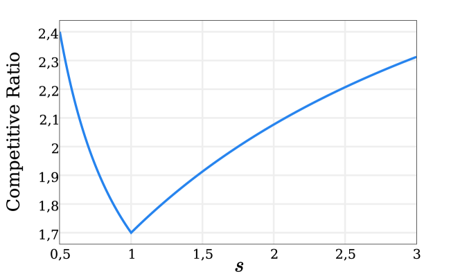
Figure 1: Competitive ratio of $\mathcal{A}_{s}$ as a function of $s$, with $\beta=0.3$.

We obtain the optimal deterministic online algorithm by setting $s=1$, named as Break-Even Economic Dispatching for problem $\textbf{FS-PAED}^{k}$ (BED-$k$). The algorithm switches from local generation to grid electricity procurement when the accumulated local generation deficit seen so far just equals the peak charge, thus the name “break-even dispatching”. We summarize the algorithm BED-$k$ into Algorithm 1, and characterize its competitive ratio in the following theorem.

Theorem 3.2.

The competitive ratio of BED-$k$ is given by

$$\mathbf{CR}\left(\mathbf{BED-}k\right)=2-\beta.$$

This also gives the price of uncertainty suffered by all deterministic online algorithms, i.e.,

$$\mathbf{PoU}_{\mbox{det}}=\min_{\mbox{all deterministic }\mathcal{A}_{s}}\mathbf{CR}\left(\mathcal{A}_{s}\right)=2-\beta.$$

Algorithm 1 BED-$k$: Optimal deterministic online algorithm for $\textbf{FS-PAED}^{k}$

0:  $p_{m}$,$p_{g}$,$p_{e}(t)$,$e^{k}(t)$

0:  $u^{k}(t)$,$v^{k}(t)$

1:  $\zeta=0$, $\tau=1$

2:  while $\tau\in\mathcal{T}$ do

3:     if $\exists\iota<\tau$ such that $v^{k}(\iota)=1$ then

4:        $v^{k}(\tau)=e^{k}(\tau)$, $u^{k}(\tau)=0$

5:     else

6:        $\zeta=\zeta+(p_{g}-p_{e}(\tau))e^{k}(\tau)$

7:        if $\zeta<p_{m}$ then

8:           $u^{k}(\tau)=e^{k}(\tau)$, $v^{k}(\tau)=0$

9:        else

10:           $v^{k}(\tau)=e^{k}(\tau)$, $u^{k}(\tau)=0$

11:        end if

12:     end if

13:     $\tau=\tau+1$

14:  end while

We remark that the optimal deterministic algorithm is easy to implement and achieves the minimum possible competitive ratio for problem $\textbf{FS-PAED}^{k}$. Next, we proceed to design optimal randomized algorithm for the problem.

3.2.2 An Optimal Randomized Online Algorithm

Recall that for the purpose of designing randomized online algorithms with the minimum competitive ratio for problem $\textbf{FS-PAED}^{k}$, it suffices to consider algorithm $\mathcal{A}_{f}$ where $f$ represents the probability distribution by which we generate the algorithm-specific threshold $s$. Based on the analysis for deterministic online algorithms in Sec. 3.2.1, we can find the competitive ratio of $\mathcal{A}_{f}$ by solving the following optimization problem:

$$\mathbf{CR}\left(\mathcal{A}_{f}\right)=\max_{\sigma}\mathbf{E}_{f}\left[h\left(\mathcal{A}_{f},\sigma\right)\right]=\max_{\sigma}\int_{s}h\left(\mathcal{A}_{s},\sigma\right)f(s)ds.$$ (8)

In the following, we first design a randomized online algorithm by specifying a particular probability distribution and compute its competitive ratio. We then leverage Yao’s Principle [22] to obtain a lower bound of the competitive ratio of any randomized algorithm. We will see the competitive ratio of our proposed online algorithm matches the lower bound, establishing its optimality. The result thus also characterizes the price of uncertainty suffered by all randomized online algorithms.

We propose a randomized online algorithm by choosing the distribution for $s$ as

$$f^{*}(s)=\begin{cases}\frac{e^{s}}{e-1+\beta},&\mbox{when }s\in[0,1];\\ \frac{\beta}{e-1+\beta}\delta(0),&\mbox{when }s=\infty;\\ 0,&\mbox{otherwise}.\end{cases}$$ (9)

We summarize the resulting randomized online algorithm in to Algorithm 2, named as Randomized Economic Dispatching for problem $\textbf{FS-PAED}^{k}$ (RED-$k$). Its competitive ratio is characterized in the following theorem.

Theorem 3.3.

With the distribution given by $f^{*}(s)$ in (9), the competitive ratio of RED-$k$ is given by

$$\mathbf{CR}\left(\mathbf{RED-}k\right)=\frac{e}{e-1+\beta}.$$

Proof 3.4.

When $\sigma\leq 1$,

$$\int_{s}h(s,\sigma)f^{*}(s)ds =\int_{0}^{\sigma}(1+\frac{1-\sigma+s}{\sigma}(1-\beta))\frac{e^{s}}{e-1+\beta}ds$$

$$+\int_{\sigma}^{1}\frac{e^{s}}{e-1+\beta}ds+\frac{e}{e-1+\beta}$$

$$=1+\int_{0}^{\sigma}\frac{1-\sigma+s}{\sigma}(1-\beta)\frac{e^{s}}{e-1+\beta}ds$$

$$=1+\frac{1-\beta}{e-1+\beta}$$

$$=\frac{e}{e-1+\beta}$$

When $\sigma>1$,

$$\int_{s}h(s,\sigma)f^{*}(s)ds =\int_{0}^{1}(1+\frac{1-\sigma+s}{\sigma}(1-\beta))\frac{e^{s}}{e-1+\beta}ds$$

$$+\int_{1}^{\sigma}\frac{e^{s}}{e-1+\beta}ds$$

$$+\int_{\sigma}^{+\infty}(1+\frac{(\sigma-1)(1-\beta)}{(\sigma-1)\beta+1})\frac{\beta}{e-1+\beta}$$

$$=1+\frac{1}{e-1+\beta}\frac{1-\beta}{(\sigma-1)\beta+1}(1+(\sigma-1)\beta)$$

$$=1+\frac{1-\beta}{e-1+\beta}$$

$$=\frac{e}{e-1+\beta}$$

Then

$$\max_{\sigma}\int_{s}h(s,\sigma)f^{*}(s)ds=\frac{e}{e-1+\beta}.$$

The proof is completed.

Algorithm 2 RED-$k$: Optimal randomized online algorithm for $\textbf{FS-PAED}^{k}$

0:  $p_{m}$,$p_{g}$,$p_{e}(t)$,$e^{k}(t)$

0:  $u^{k}(t)$,$v^{k}(t)$

1:  generate $s$ according to the probability distribution specified in (9)

2:  $\zeta=0$, $\tau=1$

3:  while $\tau\in\mathcal{T}$ do

4:     if $\exists\iota<\tau$ such that $v^{k}(\iota)=1$ then

5:        $v^{k}(\tau)=e^{k}(\tau)$, $u^{k}(\tau)=0$

6:     else

7:        $\zeta=\zeta+(p_{g}-p_{e}(\tau))e^{k}(\tau)$

8:        if $\zeta<s\cdot p_{m}$ then

9:           $u^{k}(\tau)=e^{k}(\tau)$, $v^{k}(\tau)=0$

10:        else

11:           $v^{k}(\tau)=e^{k}(\tau)$, $u^{k}(\tau)=0$

12:        end if

13:     end if

14:     $\tau=\tau+1$

15:  end while

Now we leverage Yao’s Principle [22] to obtain a lower bound for the competitive ratio of any randomized online algorithm. The idea is to choose a probability distribution for $\sigma$, denoted by $g(\sigma)$, and compute the competitive ratio of the best deterministic online algorithm for this input. Yao’s Principle says that the computed ratio is a lower bound for any randomized online algorithm. The particular distribution we use is given by

$$g^{*}(\sigma)=\begin{cases}\frac{e}{e-1+\beta}\sigma e^{-\sigma},&\mbox{when }\sigma\in[0,1],\\ \frac{e}{e-1+\beta}[(\sigma-1)\beta+1]e^{-\sigma},&\mbox{otherwise.}\end{cases}$$ (10)

The lower bound is characterized in the following lemma.

Theorem 3.5.

For any randomized online algorithm $\mathcal{A}_{f}$ for problem $\textbf{FS-PAED}^{k}$, we have

$$\mathbf{CR}\left(\mathcal{A}_{f}\right)\geq\frac{e}{e-1+\beta}.$$

The competitive ratio of algorithm RED-$k$ achieves this lower bound and thus is optimal. Consequently, the price of uncertainty suffered by all randomized online algorithms is given by

$$\mathbf{PoU}_{\mbox{ran}}=\min_{\mbox{all randomized }\mathcal{A}_{f}}\mathbf{CR}\left(\mathcal{A}_{f}\right)=\frac{e}{e-1+\beta}.$$

Proof 3.6.

When $s\leq 1$,

$$\int_{\sigma}h(s,\sigma)g^{*}(\sigma)d\sigma =\int_{0}^{s}g^{*}(\sigma)d\sigma+\int_{s}^{1}(1+\frac{(1-\sigma)s}{z})g^{*}(\sigma)d\sigma$$

$$+\int_{1}^{+\inf}(1+\frac{s(1-\beta)}{(\sigma-1)\beta+1})g^{*}(\sigma)d\sigma$$

$$=1+\frac{e(1-\beta)}{e-1+\beta}\cdot$$

$$\left[\int_{s}^{1}(1-\sigma+s)e^{-\sigma}dz+\int_{1}^{+\inf}se^{-\sigma}d\sigma\right]$$

$$=1+\frac{e(1-\beta)}{e-1+\beta}e^{-1}$$

$$=\frac{e}{e-1+\beta}$$

When $s>1$,

$$\int_{\sigma}h(s,\sigma)g^{*}(\sigma)d\sigma =\int_{0}^{1}g^{*}(\sigma)d\sigma$$

$$+\int_{1}^{s}(1+\frac{(\sigma-1)(1-\beta)}{(\sigma-1)\beta+1})g^{*}(\sigma)d\sigma$$

$$+\int_{s}^{+\inf}(1+\frac{s(1-\beta)}{(\sigma-1)\beta+1})g^{*}(\sigma)d\sigma$$

$$=1+\frac{e(1-\beta)}{e-1+\beta}\cdot$$

$$\left[\int_{1}^{s}(\sigma-1)e^{-\sigma}d\sigma+\int_{s}^{+\inf}se^{-\sigma}d\sigma\right]$$

$$=1+\frac{e(1-\beta)}{e-1+\beta}e^{-1}$$

$$=\frac{e}{e-1+\beta}$$

Then

$$\min_{s}\left[\int_{\sigma}h(s,\sigma)g^{*}(\sigma)d\sigma\right]=\frac{e}{e-1+\beta}.$$

The proof is completed.

Remark: (i) In the deterministic online algorithm, setting $s=1$ means that the microgrid will start to buy electricity from the grid until the break-even condition is met. Similar to the ski rental problem [12], the break-even point turns out to be the best balance between being aggressive and conservative. (ii) The vigilant readers may notice that $f^{*}(s)$ is the same distribution that was adopted in solving the classic Bahncard problem [9], which is indeed similar to problem $\textbf{FS-PAED}^{k}$ we study in this section. The basic version of $\textbf{FS-PAED}^{k}$, however, is different from Bahncard problem in the sense that the discounted price ($p_{e}(t)$ in this paper) is time varying. (iii) Different from the neat tricks used in [9] to prove the optimality of the proposed randomized online algorithm [9], we leverage Yao’s Principle to prove the optimality of our proposed algorithm RED-$k$ for problem $\textbf{FS-PAED}^{k}$. Exploiting the similarity of the two problems, our approach can also be applied to establish optimality of the proposed algorithm for the Bahncard problem in [9].

3.3 From Problem $\textbf{FS-PAED}^{k}$ to Problem FS-PAED

In this section, we design online deterministic and randomized algorithms for FS-PAED based on those of $\textbf{FS-PAED}^{k}$.

3.3.1 Net Demand Layering

For each time slot $t$, we divide the demand $e(t)$ into multiple layers such that the demand of each layer is either $1$ or $0$, as shown in Fig. 2. Recall that $e(t)$ is assumed to take non-negative integer values. We denote the sub-problem of satisfying the demand of each layer as $\textbf{FS-PAED}^{k},k=1,2,...$, and we can apply the online algorithms BED-$k$ and RED-$k$ for each sub-problem.

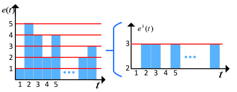
Figure 2: An example of decomposing the demand into multiple layers and a microscopic view of layer 3

3.3.2 Optimal Online Algorithms for FS-PAED

After layering, a bunch of sub-problems $\textbf{FS-PAED}^{k}$ are obtained. However, unlike $\textbf{FS-PAED}^{k}$, the net demand of FS-PAED in some time slots can exceed the capacity of local generation, which makes it infeasible to ignore the whole picture when conquering each layer independently. For example, suppose the generation capacity is 4 for the case shown in Fig. 2. Even though the break even points are not reached for all the layers in time slot 2, it is infeasible to set $u^{k}(2)=1$ for all the layers (A capacity of 5 is needed to do so). Thus by taking into account the capacity constraint, we need to determine for which layers the demand should be satisfied by the grid while still keeping the algorithm competitive.

An obvious but critical observation is that the demands in the lower layers are denser than those in the upper layers. In addition, after being charged for the peak, we expect more demands to come to enjoy the cheap grid electricity. Consequently, it is always more economic to use the grid electricity to satisfy the denser demands, i.e., the lower layers. In other words, in the proper algorithm design, the layers below $(e(t)-C)^{+}$ should always be satisfied by the grid. Meanwhile, for the layers above $(e(t)-C)^{+}$, if the demand is already satisfied by the grid, the online algorithm continues to acquire the electricity from the grid; otherwise, Algorithm BED-$k$ or RED-$k$ is applied with the same value $s$ for all layers to obtain the sub-solutions. The solution is finally obtained by combining the sub-solutions. We summarize the resulting deterministic an randomized online algorithms, named as BED and RED, in Algorithm 3 and 4, respectively.

Algorithm 3 BED: Optimal deterministic online algorithm for FS-PAED

0:  $C$,$p_{m}$,$p_{g}$,$p_{e}(t)$,$e(t)$

0:  $u(t)$,$v(t)$

1:  while $\tau\in\mathcal{T}$ do

2:     A threshold: $\varsigma=(e(\tau)-C)^{+}$.

3:     For the layers below $\varsigma$, $v^{k}(\tau)=1$, $u^{k}(\tau)=0$

4:     For the layers above $\varsigma$, run BED-$k$ to obtain $u^{k}(\tau)$ and $v^{k}(\tau)$.

5:     $u(\tau)=\sum_{k}u^{k}(\tau)$, $v(\tau)=\sum_{k}v^{k}(\tau)$

6:     $\tau=\tau+1$

7:  end while

Algorithm 4 RED: Optimal randomized online algorithm for FS-PAED

0:  $C$,$p_{m}$,$p_{g}$,$p_{e}(t)$,$e(t)$

0:  $u(t)$,$v(t)$

1:  while $\tau\in\mathcal{T}$ do

2:     A threshold: $\varsigma=(e(\tau)-C)^{+}$.

3:     For the layers below $\varsigma$, $v^{k}(\tau)=1$, $u^{k}(\tau)=0$

4:     For the layers above $\varsigma$, run RED-$k$ with the same randomized parameter $s$ to obtain $u^{k}(\tau)$ and $v^{k}(\tau)$.

5:     $u(\tau)=\sum_{k}u^{k}(\tau)$, $v(\tau)=\sum_{k}v^{k}(\tau)$

6:     $\tau=\tau+1$

7:  end while

We demonstrate a toy example of the solution given by BED in Fig. 3. For simplicity, we assume the break-even condition is firstly met when the third nonzero demands comes for all the layers, and the local capacity is $4$. We use different colors to demonstrate by which source and for what reason one unit of demand is satisfied. Even though the example is simple, it demonstrates two important and provable properties of BED: (i) For each layer, it will continue to use the grid after it uses it once, and (ii) when one layer uses the grid, all the layers below it use the grid too. The first property makes the solution and cost structure similar to that of BED-$k$, while the second property makes the peak of $v(t)$ equal to the sum of the peaks of $v^{k}(t)$, i.e., $\max_{t}\sum_{k}v^{k}(t)=\sum_{k}\max_{t}v^{k}(t)$. The two properties allow us to leverage the results in Sec. 3.2 to establish the competitive ratios of BED and RED.

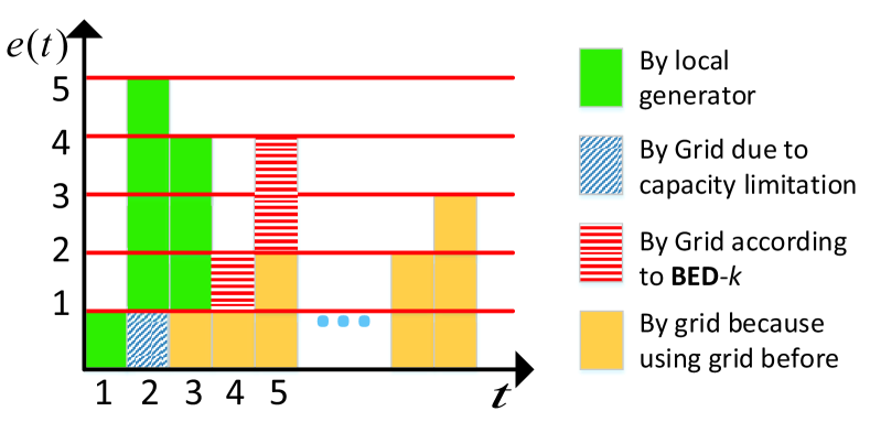
Figure 3: Demonstration of BED with $C=4$, different colors denoting different strategies of the algorithm.

Theorem 3.7.

The competitive ratios of BED and RED are given by

$$\mathbf{CR}\left(\mathbf{RED}\right)=2-\beta,\;\;\;\mbox{and \;\;\;}\mathbf{CR}\left(\mathbf{RED}\right)=\frac{e}{e-1+\beta}.$$

Further, no other deterministic and randomized online algorithm can achieve a smaller competitive ratio.

Proof 3.8.

Firstly, if the given input violates the capacity constraints, we can construct a new input respecting the capacity constraints, by sequently removing the demand exceeding the capacity and the following demands in the same layer (like the first layer from time slot 2 in Fig 3). Then compared with the original input, the online cost and offline cost are reduced by the same amount, which leads to a larger competitive ratio. Then we only need to focus on the input whose demand is always smaller than the capacity.

Furthermore, due to the second property of the algorithm, we can have $\max_{t}\sum_{k}v^{k}(t)=\sum_{k}\max_{t}v^{k}(t)$, and $\begin{cases}u(t)=\sum_{k}u^{k}(t)\\ v(t)=\sum_{k}v^{k}(t)\end{cases}$. Then $\textsf{Cost}(\boldsymbol{u},\boldsymbol{v})=\sum_{k}\textsf{Cost}({\boldsymbol{u}}^{k},{\boldsymbol{v}}^{k})$. This property still holds for the offline cost. We denote $\tilde{r}$ as the competitive ratio for each layer, meaning

$$\textsf{Cost}({\boldsymbol{u}}^{k},{\boldsymbol{v}}^{k})\leq\tilde{r}\text{Cost}^{k}_{\text{off}},\forall k.$$

Then by summing the above inequality on $k$, we can have

$$\textsf{Cost}(\boldsymbol{u},\boldsymbol{v})\leq\tilde{r}\text{Cost}_{\text{off}}.$$

For BED, $\tilde{r}=2-\beta$ and for RED, $\tilde{r}=\frac{e}{e-1+\beta}$ for the randomized case, which establish the upper bound of the competitive ratios.

Furthermore, note that $\textbf{FS-PAED}^{k}$ is a special case of FS-PAED. Since we cannot obtain smaller competitive ratios for $\textbf{FS-PAED}^{k}$, we cannot obtain smaller competitive ratios for FS-PAED.

The proof is completed.

In the next subsection, we discuss an intriguing consequence of local generation capacity on the online algorithms’ performance.

3.4 Critical Local Generation Capacity

The peak-aware economic dispatching aims at minimizing the sum of the peak charge (the term $p_{m}\max_{t\in\mathcal{T}}v(t)$ in (1)) and the volume charge (as the remaining part in (1)). The local generator provides the microgrid an option to use more expensive electricity (increase the volume charge) to reduce the peak (decrease the peak charge). An optimal solution is achieved with the best tradeoff between the two. Given an input, there is a threshold $\tilde{C}$, the demand below which should be satisfied by the grid and above which by the local generator. $\tilde{C}$ can be obtained by solving FS-PAED in an offline fashion without considering capacity constraint. It means that the optimal offline solution will not use the additional capacity even if it is larger than $\tilde{C}$.

We now discuss the impact of increasing local generation capacity $C$ on the performance of offline and online algorithms. The offline algorithm will use full local capacity until $C$ reaches $\tilde{C}$, and it will not use local capacity further beyond $\tilde{C}$. As such, one can expect that the operating cost of the offline algorithm is non-increasing as $C$ increases. Meanwhile, the online algorithm, without knowing $\tilde{C}$ and with the tendency of reducing the peak with more expensive electricity, will try to exploit the whole capacity until it finds the break even point, which turns out to be less economic and deviates more from the optimal solution. As a result, for the online algorithm, larger capacity may incur higher operating cost. We provide a concrete case-study by real world traces to confirm the above observation in Sec. 5.

Overall, we believe the above insights are important for microgrid operators to (a) determine the amount of local generation to invest in order to maximize the economic benefit, and (b) understand the importance of demand/generation prediction when performing peak-aware economic dispatching in microgrids.

4 Slow-Responding Generator Case

This section considers the slow-responding generator scenario, in which the ramping up/down constraints in (2d)-(2d) are non-negligible. We remark that we can still optimally solve the problem PAED with these constraints in the offline manner by convex optimization techniques.

In the following analysis, we assume $R^{\textsf{u}}=R^{\textsf{d}}=R$ and define $\Gamma=\lceil\frac{C}{R}\rceil$. Then, it takes $\Gamma$ time slots for the local generator’s output to ramp up from zero to full capacity or down from full capacity to zero. Considering the time scale of our problem (say, 15 minutes for each time slot) and the microgrid scenario (high efficiency of local generators), $\Gamma$ is conceivable to be small. We assume $\Gamma$ is no larger than 5, meaning it roughly takes no more than 75 minutes for local generator to fully ramp up.

We first show a result highlighting the difficulty introduced by the ramping constraints in designing competitive online economic dispatching algorithms.

Proposition 4.9.

Any online algorithm for problem PAED without future information, i.e., at time $t$ the algorithm only have knowledge of $\left\{e(\tau),p_{e}(\tau)\right\}_{\tau=1}^{t}$, has a competitive ratio at least $\frac{p_{m}(C-R)+p_{g}R}{p_{g}(R\Gamma(\Gamma-1)+C)}$.

When $\Gamma$ is $5$ and $p_{m}$ is 100 times of $p_{g}$, a back-of-envelop calculation reveals that the lower bound of the competitive ratio can be as large as $20$. This result shows that the ramping constraints will make any online algorithm design less attractive as the worst performance can be rather bad. The conventional method to address this problem is to put additional constraints on the input to obtain algorithms with reasonable performance guarantee [16]. In this paper, we propose to handle the challenge incurred by ramping constraints by a different approach; that is to empower the algorithm with a limited looking ahead window.

4.1 An Effective Online Algorithm by a Limited Looking-ahead Window

Motivated by the development of prediction algorithms [17, 24], we assume that a limited looking ahead window with size of $\Delta=\Gamma-1$ is available, which means that at time $t$ we can know the input from $t+1$ to $t+\Delta$ in advance. In this section, we devise an online algorithm by leveraging such looking ahead information as well as the results in Sec 3. We name the proposed algorithm as NRBF (Neutralize Ramping constraint By Future information). We denote the online solutions we obtain for PAED by NRBF as $\tilde{u}(t),\tilde{v}(t)$.

In NRBF , we first solve problem FS-PAED by relaxing the ramping constraints from problem PAED and denote the solutions obtained by algorithms BED or RED as $u(t)$ and $v(t)$. We then adjust them to obtain online solutions for PAED that satisfy the ramping constraints. Specifically, we compute $\tilde{u}(t)$ as

$$\tilde{u}(t)=\max\{\tilde{u}(t-1)-R,u(t+i)-iR|i=0,1,..,\Delta\},$$

and $\tilde{v}(t)=\max\left(e(t)-\tilde{u}(t),0\right)$.

The following lemma shows that the ramping constraints are respected by NRBF.

Lemma 4.10.

The solutions by NRBF satisfy the generator’s ramping constraints, i.e.,

$$|\tilde{u}(t+1)-\tilde{u}(t)|\leq R.$$

Proof 4.11.

By the obtainment of $\tilde{u}(t+1)$, we can have $\tilde{u}(t+1)\geq\tilde{u}(t)-R$, i.e

$$\tilde{u}(t)-\tilde{u}(t+1)\leq R$$

Next, we prove $\tilde{u}(t+1)-\tilde{u}(t)\leq R$ for two cases.

Firstly, if $\tilde{u}(t+1)=(\tilde{u}(t)-R)^{+}$, the conclusion holds obviously.

Secondly, if for some $i^{*}\in[0,w-1]$ such that $\tilde{u}(t+1)=u(t+1+i^{*})-i^{*}R$, we can have

$$\tilde{u}(t+1) =\max\{0,u(t+1+i)-iR|i\in[0,\Delta]\}$$

$$=\max\{0,u(t+1+i)-(i+1)R+R|i\in[0,\Delta]\}$$

$$=\max\{0,u(t+j)-jR|j\in[1,\Gamma]\}+R\}$$

$$=\max\{0,u(t+j)-jR|j\in[1,\Delta]\}+R\}$$

The last step is due to the fact that $u(t+w)\leq C\leq wR$. and since $\tilde{u}(t)=\max\{0,\tilde{u}(t-1)-R,\max\{u(t+j)-jR|i\in[0,w-1]\}\}$, we can have $\tilde{u}(t)\geq\max\{0,u(t+j)-jR|j\in[0,\Delta]\}\geq\{0,u(t+j)-jR|j\in[1,\Delta]\}$.

Then it’s easy to see that $\tilde{u}(t+1)\leq\tilde{u}(t)+R$, i.e $\tilde{u}(t+1)-\tilde{u}(t)\leq R,$ which means the ramping up constraint is satisfied and the proof is completed.

Meanwhile, we can have $\tilde{v}(t)\leq v(t)$, meaning the peak charge is upper bounded by that of the fast responding scenario. We leverage this observation to show the competitiveness of NRBF, as shown in Theorem 4.12.

Theorem 4.12.

The competitive ratio of NRBF satisfies

$$\mathbf{CR}\left(\mbox{{NRBF} }\right)\leq\begin{cases}\Gamma\left(2-\beta\right),&\mbox{if }u(t),\,v(t)\mbox{ are obtained by {BED}};\\ \Gamma\frac{e}{e-1+\beta},&\mbox{if }u(t),\,v(t)\mbox{ are obtained by {RED}}.\end{cases}$$

Proof 4.13.

According to the algorithm we can easily get

Lemma 4.14.

For $\tilde{u}(t)$,$\tilde{v}(t)$ obtain by NRBF , we can have $\tilde{v}(t)\leq v(t)$, and thus $\max_{t}\tilde{v}(t)\leq\max_{t}v(t)$

We denote the online cost of NRBF as $\tilde{C}_{\textrm{on}}$ and the optimal offline cost of the same problem as $\tilde{C}_{\textrm{off}}$. For the problem without ramping constraints, we denote the online cost of BED or RED as $C_{\textrm{on}}$ and the optimal offline cost of the same problem as $C_{off}$. We can directly have $\tilde{C}_{\textrm{off}}\geq C_{\textrm{off}}$. Then

$$\frac{\tilde{C}_{\textrm{on}}}{\tilde{C}_{\textrm{off}}} \leq\frac{\tilde{C}_{\textrm{on}}}{C_{\textrm{off}}}$$

$$=\frac{\tilde{C}_{\textrm{on}}}{C_{\textrm{on}}}*\frac{C_{\textrm{on}}}{C_{\textrm{off}}}$$

$$\leq\frac{\tilde{C}_{\textrm{on}}}{C_{\textrm{on}}}*\mathcal{CR}$$

If $\frac{\tilde{C}_{\textrm{on}}}{C_{\textrm{on}}}\leq 1$, this theorem holds obviously; otherwise, we denote $\begin{cases}\tilde{C}_{\textrm{on}}=\tilde{C}_{\textrm{on}}^{l}+\tilde{C}_{\textrm{on}}^{g}\\ C_{\textrm{on}}=C_{\textrm{on}}^{l}+C_{\textrm{on}}^{g}\end{cases}$, where the superscripts $l$ and $g$ represent the costs from local generators and external grid respectively.

By Lemma 4.14, we can have $\tilde{C}_{\textrm{on}}^{g}\leq C_{\textrm{on}}^{g}$; then

$$\frac{\tilde{C}_{\textrm{on}}}{C_{\textrm{on}}}\leq\frac{\tilde{C}_{\textrm{on}}^{l}}{C_{\textrm{on}}^{l}}$$

Next we obtain an upper bound for $\frac{\tilde{C}_{\textrm{on}}^{l}}{C_{\textrm{on}}^{l}}$ by modifying the input a little bit. We expand each time slot to one segment by inserting $\frac{u(t)}{R}$ intervals with $0$ demand before $t$ and another $\frac{u(t)}{R}$ intervals with $0$ demands after $a(n)$. Then, the online cost stays the same for the problem without ramping constraints. Furthermore, the online cost for the problem with ramping constraints increases.

For the $m^{th}$ segment,$C_{\textrm{on}}^{l}(m)=p_{g}u(m)$, while $\tilde{C}_{\textrm{on}}^{n}(m)=p_{g}(\sum_{i=1}^{\Gamma-1}iR+u(m)+\sum_{i=1}^{\Gamma-1}iR)\leq p_{g}*u(m)\Gamma$; meaning for any $m$ we can have

$$\frac{\tilde{C}_{\textrm{on}}^{l}(m)}{C_{\textrm{on}}^{n}(m)}\leq\Gamma$$

Then

$$\frac{\tilde{C}_{\textrm{on}}^{l}}{C_{\textrm{on}}^{l}} =\frac{\sum_{m}\tilde{C}_{\textrm{on}}^{l}(m)}{\sum_{m}C_{\textrm{on}}^{l}(m)}$$

$$\leq\Gamma$$

Further we can have $\frac{\tilde{C}_{on}}{\tilde{C}_{off}}\leq\frac{C}{R}\mathcal{CR}$, which completes the proof.

Remark: Small values of $\Gamma$, which mean the ramping constraints are less strict, will lead to a small bound on the competitive ratio. Moreover, $\Gamma=1$ indicates that the generator output can ramp up to its full capacity in one time slot and the ramping constraints vanish, thereby we do not need any future information ($\Delta=0$) and the competitive ratio is exactly the same with that of the fast-responding generator scenario.

5 Experimental Results

We carry out numerical experiments using real-world traces to scrutinize the performance of our online algorithms under various practical settings. Our purpose is to investigate (i) the competitiveness of online algorithms in comparison with the optimal offline one, (ii) the necessity of peak-awareness in economic dispatching of microgrids, and (iii) the performance of online algorithms under various parameter settings.

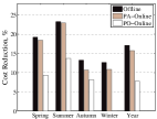
Figure 4: Cost reduction for different seasons and the whole year

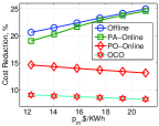
Figure 5: Cost reduction vs $p_{m}$

5.1 Experimental Setup

Electricity demand and renewable generation traces. We set the length of one billing circle as one month. We use the actual electricity demand of a college in San Francisco; its yearly demand is about $154\textrm{GWh}$ [1]. We inject renewable energy supply sources by a wind power trace of a nearby offshore wind station outside San Francisco with a total installed capacity of $12\textrm{MW}$ [2]. We then construct the net demand by subtracting the output level of the wind from the college electricity demand.

Energy source parameters. The electricity price $p_{e}(t)$ and peak price $p_{m}$ are set based on the tariffs from PG&E[5] and $p_{m}=17.56\$/\textrm{KWh}$ while the electricity rate $p_{e}(t)$ varies from $0.056\$/\textrm{KWh}$ to $0.232\$/\textrm{KWh}$ for off-, mid-, and on-peak periods in different seasons. We set the unit cost of local generation $p_{g}$ according to the monthly price of natural gas. Notably, the value of $p_{g}$ could be less than $p_{e}(t)$ for some on-peak intervals. In such situations, generator plays its role not only by cutting off the peak but also by providing cheaper electricity as well. Finally, if not specified, the capacity of the local generator is set to be $C=15\textrm{MWh}$, which is around $60\%$ of the peak net demand.

Cost benchmark. We use the cost incurred by only procuring electricity from the external grid, i.e., $v(t)=e(t)$, as the benchmark. We demonstrate cost reduction to show the benefit of employing local generation units and the effectiveness of algorithms. The cost reduction originates from the cheaper electricity (in some on-peak intervals) and peak cut-off by local generators.

Comparison of algorithms. We compare our proposed peak-aware online economic dispatching (PA-Online) algorithms with (i) the optimal peak-aware offline solution (OFFLINE) to evaluate the performance of the online algorithms, and (ii) the peak-oblivious online algorithms (PO-Online) in [14] and online convex optimization approach (OCO) in [16] to investigate the importance of peak-awareness. We remark that both schemes in  [14, 16] are peak-oblivious as they only consider volume charge but ignore peak charge.

The results reported in Secs. 5.2- 5.4 cover the fast-responding generator scenarios and Sec. 5.7 is devoted to the slow-responding generator scenario.

5.2 Benefits of Employing Local Generators

Purpose. The purpose of this experiment is two-fold. First, compare the potential savings of microgrid in different seasons, in which the demand pattern, the wind output, and the cost parameters differ. Second, compare the cost reduction of peak-aware algorithms against peak-oblivious ones. The results are shown in Fig. 5.

Observations. The most notable observations from Fig. 5 are the following. First of all, the cost reduction varies over seasons and the most significant one occurs in the summer. This is because the gas price is lower and the grid electricity price is higher in the summer than those of the other seasons, thus employing local generators brings more benefit. Second, the performance of our proposed PA-Online is superior than PO-Online algorithm. In particular, PO-Online cannot reduce the cost in the winter, but our algorithm PA-Online can still achieve cost reduction. The reason is that, as $p_{g}>p_{e}(t)$ always holds in the winter, PO-Online algorithm always purchases cheaper electricity from the gird, which gives no cost reduction as compare to the benchmark strategy. In contrast, our PA-Online algorithm reduces the cost by exploiting (the expensive) local generation to reduce the peak demand served by the external grid, and consequently our algorithm can save operating cost. On average, PA-Online reduces the annual cost by $15.7\%$, while PO-Online reduces the cost only by $8.17\%$. Third, the performance of PA-Online in practice is close to that of the offline optimal.

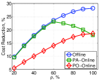
Figure 6: Cost reduction vs $\rho$

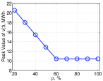
Figure 7: Peak value of $v(t)$ vs $\rho$

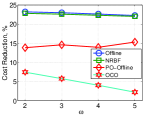
Figure 8: Cost reduction vs $\Gamma$

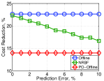
Figure 9: Cost reduction vs prediction error

5.3 The Performance of PA-Online under Different Peak Prices

Purpose. To validate the peak charge is non-negligible which motivates our study, we evaluate the performance of our peak-aware algorithm and that of the peak-oblivious one under different peak prices. In particular, in Fig. 5, we depict the cost reduction of different algorithms with the peak price $p_{m}$ varying from $12.29\$/\textrm{KWh}$ to $21.07\$\textrm{/KWh}$.

Observations. When $p_{m}$ increases, the cost reduction of our PA-Online algorithm increases and is close to the offline optimal, while the reductions of the two peak oblivious algorithms decrease. This observation shows that our PA-Online algorithm is more effective and the cost reduction is more significant for microgrids with high peak prices.

5.4 The Performance of PA-Online under Different Local Generation Capacities

Purpose. At first glance, one may imagine that larger local generator leads to larger design space and thus larger cost reduction is expected. However, as discussed in Sec. 3.4, this is not the case for online algorithms that do not have the complete future knowledge of price and demand. We carry out an experiment to verify and elaborate the observation. For convenience, we define $\rho=C/\max{e(t)}$ as the ratio of local generation capacity over the peak net demand and change $\rho$ from $20\%$ to $100\%$. The result is shown in Fig. 7.

Observations. The results for OFFLINE and PO-Online algorithms follow the intuition that more local capacity brings more cost reduction. For PA-Online, however, we observe that the cost reduction increases when $\rho$ increases from $20\%$ to $60\%$, and degrades as $\rho$ continues to increase from $60\%$ to $100\%$. As we discussed in Sec. 3.4, there exists a critical local generation capacity $\tilde{C}$ beyond which the peak charge and the overall cost will not decrease further. In Fig. 7, we report the peak grid demand $\max{v(t)}$ versus $\rho$ just for OFFLINE algorithm. Results show that the peak value of $v(t)$ does not decrease as $\rho$ increases from $60\%$ to $100\%$, evincing that $\tilde{C}$ is about $60\%$ of the maximum demand in this case. The online algorithm, however, is unaware of $\tilde{C}$. As discussed in Sec. 3.4, $\tilde{C}$ can be computed by solving problem FS-PAED in an offline manner.

The online algorithm, without knowing $\tilde{C}$ and with the tendency of reducing the peak charge by using more expensive local generation, will try to exploit the entire local generation capacity until the cost-benefit break even point is reached, which turns out to be less economic and deviate from the offline optimal. As a result, for the online algorithm, larger capacity may incur higher operating cost, as shown in Fig. 7.

This experiment, together with the discussions in Sec. 3.4, show that it is important for the microgrid operator to set the local generation capacity right at $\tilde{C}$ to cope with online algorithms to achieve maximum cost reduction. A possible way to set $\tilde{C}$ is to use the historical data as the input to the offline algorithm and obtain the critical capacity.

5.5 The Performance of RED

Purpose. In this part, we compare the empirical performance of the deterministic online algorithm BED and randomized online algorithm RED under different local capacities. The cost of RED is computed by running the algorithm 1000 times and taking the average.

Observations. Even though RED is better than BED in terms of competitive ratio, it is not always the case empirically because the competitive ratio only characterizes the performance in the worst case. As we can see, when $\rho$ is less than 80%, BED outperforms RED while the other way around if $\rho$ is larger than 80%. Furthermore, when $\rho$ increases from 80% to 100%, the performance of BED degrades drastically, while the cost reduction of RED almost remains the same. This observation indicates that, to ensure that BED has good performance, we need to carefully determine the local capacity but additional local capacity will not harm RED much, which can be viewed as another advantage of RED.

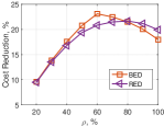
Figure 10: Comparison of RED and BED under different local capacities

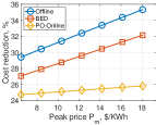
Figure 11: Cost reduction with different peak price on a small microgrid testbed

5.6 Empirical Evaluations Using Traces from a Real-world Small-scale Microgrid

Purpose. In this simulation, we replace the previous trace with a new one, which is from a test-bed building at College of Engineering Center for Environmental Research and Technology of UC Riverside and spans three months from May to July. The building has 20 office rooms, 2 conference rooms, one large open area with cubicles, and 7 other miscellaneous rooms. The building HVAC system consists of 16 packaged rooftop units. In addition to its small scale, the building is connected to solar PV and several charging stations, both of which introduce additional demand uncertainties. As a result, the demand fluctuates more than the previous data set we use. The simulation result is shown in Fig 11.

Observations. On this new data set, the cost reduction is more significant (at least 40% for the offline case) than the previous results and will increase with larger peak price $p_{m}$. This result indicates that peak-aware scheduling is more beneficial with more fluctuating demand and larger peak prices.

5.7 The Impact of Ramping Constraints

Purpose. The experiment is devoted to explore the performance of our algorithm NRBF for slow-responding generators. We firstly change the ramping constraint such that $\Gamma$ increases from $2$ to $5$ and evaluate the performance of the algorithms. We recall the meaning of $\Gamma$, as defined in Sec. 4, is that it takes $\Gamma$ slots for local generators to ramp up from zero to full capacity or down from full capacity to zero. The result is demonstrated in Fig. 9.

Secondly, we relax the assumption that we can perfectly predict near future information. We add a zero mean gaussian noise to the net demand as the predicted input for our algorithm. Note that we can always satisfy unexpected demand by purchasing electricity from the external grid. We evaluate the performance of NRBF with standard deviation of the gaussian noise increasing from $0\%$ to $10\%$ of the actual demand. We use $\Gamma=4$ for the experiment and NRBF utilizes 3-slot looking ahead demand and price information. The simulation results are shown in Fig. 9.

Observations. From Fig. 9, we observe that all cost reductions decrease as ramping constraints are more strict, while the performance of NRBF is always close to the offline optimal. This shows the effectiveness of using limited prediction in combating the difficulty in online scheduling caused by ramping constraints. Moreover, Fig. 9 shows that the prediction error will degrade the performance of NRBF . However, the performance is still significantly better than the peak-oblivious scheduling.

6 Related Work

Microgrid is attracting substantial attention from both academic and industrial communities due to its economic and environmental benefits, evidenced by a number of real-world pilot microgrid projects [7].

With the penetration of renewable energy in microgrids, conventional economic dispatching approaches based on accurate demand prediction for power grid [10] are not applicable as the net demand inherits substantial uncertainty from the renewable generation and is hard to predict accurately. Online algorithm design is advocated by researchers to offer a paradigm-shrift alternative. Online convex optimization [16], Lyapunov optimization [11], and competitive analysis [14] are the main approaches adopted for online energy generation scheduling in microgrid. The authors in [14] study the unit commitment and economic dispatching problems of microgrid under the volume charging model. Our work considers economic dispatching under both the peak charging and volume charging model.

The cost minimization problem based on real-world peak charging scheme has been considered for microgird scenario in [15], by utilizing Energy Storage Systems to cut off the peak. In contrast, our work tackles the problem using local generators to shave the peak. The cost minimization with the same pricing mechanism taken into account is also studied for data centers in [21, 19], for EV charging in [23], and for content delivery in [6]. For fast-responding generator scenario, the economic dispatching problem we study in this paper can be considered as a generalization of the classic Bahncard problem [9]. The Bahncard problem and its solutions have also found application in the instance acquisition problem of cloud computing [20].

7 Conclusion and Future Work

In this paper, we devised peak-aware online economic dispatching algorithms for microgrids, with peak charging model taken into account. In the fast-responding generator scenario, we developed both deterministic and randomized online algorithms with best possible competitive ratios following a divide-and-conquer approach. Our results not only characterized the fundamental price of uncertainty for the problem, but also served as a building block for designing online algorithms for the slow-responding generator scenario, where we proposed to tackle the ramping constraints using a limited look-ahead window. In addition to sound theoretical performance guarantees, the empirical evaluations based on real-world traces also corroborated our claim on the importance of peak-awareness in scheduling.

An interesting future direction is to study the microgrid economic dispatching problem under accurate or noisy prediction of future demand and renewable generation within a limited look-ahead window.

References

- [1] California commercial end-use survey, http://capabilities.itron.com/CeusWeb.
- [2] National renewable energy laboratory, http://wind.nrel.gov.
- [3] http://www.duke-energy.com/rates/kentucky/electric.asp.
- [4] http://www.navigantresearch.com.
- [5] http://www.pge.com/nots/rates/tariffs/rateinfo.shtml.
- [6] M. Adler, R. K. Sitaraman, and H. Venkataramani. Algorithms for optimizing the bandwidth cost of content delivery. Computer Networks, 55(18):4007–4020, 2011.
- [7] M. Barnes. Real-world microgrid-an overview. In IEEE International Conference on System of Systems Engineering, 2007.
- [8] E. Fanone, A. Gamba, and M. Prokopczuk. The case of negative day-ahead electricity prices. Energy Economics, 35:22–34, 2013.
- [9] R. Fleischer. On the bahncard problem. Theoretical Computer Science, 268(1):161–174, 2001.
- [10] Z.-L. Gaing. Particle swarm optimization to solving the economic dispatch considering the generator constraints. IEEE Trans. on Power Systems, 18(3):1187–1195, 2003.
- [11] Y. Huang, S. Mao, and R. Nelms. Adaptive electricity scheduling in microgrids. In Proc. IEEE INFOCOM, pages 1142–1150, 2013.
- [12] A. R. Karlin, M. S. Manasse, L. Rudolph, and D. D. Sleator. Competitive snoopy caching. Algorithmica, 3(1-4):79–119, 1988.
- [13] S. A. Kazarlis, A. Bakirtzis, and V. Petridis. A genetic algorithm solution to the unit commitment problem. IEEE Trans. on Power Systems, 11(1):83–92, 1996.
- [14] L. Lu, J. Tu, C.-K. Chau, M. Chen, and X. Lin. Online energy generation scheduling for microgrids with intermittent energy sources and co-generation. In Proc. ACM SIGMETRICS, pages 53–66, 2013.
- [15] A. Mishra, D. Irwin, P. Shenoy, and T. Zhu. Scaling distributed energy storage for grid peak reduction. In Proc. ACM e-Energy, pages 3–14, 2013.
- [16] B. Narayanaswamy, V. K. Garg, and T. Jayram. Online optimization for the smart (micro) grid. In Proc. ACM e-Energy, pages 1–19, 2012.
- [17] J. W. Taylor, L. M. de Menezes, and P. E. McSharry. A comparison of univariate methods for forecasting electricity demand up to a day ahead. International Journal of Forecasting, 22(1):1–16, 2006.
- [18] A. Vuorinen. Planning of optimal power systems. Ekoenergo Oy Espoo, Finland, 2007.
- [19] C. Wang, B. Urgaonkar, Q. Wang, and G. Kesidis. A hierarchical demand response framework for data center power cost optimization under real-world electricity pricing. In Proc. IEEE MASCOTS, 2014.
- [20] W. Wang, B. Li, and B. Liang. To reserve or not to reserve: Optimal online multi-instance acquisition in iaas clouds. In Proc. ICAC, 2013.
- [21] H. Xu and B. Li. Reducing electricity demand charge for data centers with partial execution. In Proc. ACM e-Energy, 2014.
- [22] A. C.-C. Yao. Probabilistic computations: Toward a unified measure of complexity. In IEEE 18th Annual Symposium on Foundations of Computer Science, pages 222–227, 1977.
- [23] S. Zhao, X. Lin, and M. Chen. Peak-minimizing online EV charging. In Proc. Allerton, 2013.
- [24] T. Zhu, A. Mishra, D. Irwin, N. Sharma, P. Shenoy, and D. Towsley. The case for efficient renewable energy management in smart homes. In Proc. ACM BuildSys, pages 67–72, 2011.