MHD discontinuities in solar flares: continuous transitions and plasma heating

Abstract

The boundary conditions for the ideal MHD equations on a plane discontinuity surface are investigated. It is shown that, for a given mass flux through a discontinuity, its type depends only on the relation between inclination angles of a magnetic field. Moreover, the conservation laws on a surface of discontinuity allow changing a discontinuity type with gradual (continuous) changes in the conditions of plasma flow. Then there are the so-called transition solutions that satisfy simultaneously two types of discontinuities. We obtain all transition solutions on the basis of the complete system of boundary conditions for the MHD equations. We also found the expression describing a jump of internal energy of the plasma flowing through the discontinuity. Firstly, this allows constructing a generalized scheme of possible continuous transitions between MHD discontinuities. Secondly, it enables the examination of the dependence of plasma heating by plasma density and configuration of the magnetic field near the discontinuity surface, i.e., by the type of the MHD discontinuity. It is shown that the best conditions for heating are carried out in the vicinity of a reconnecting current layer near the areas of reverse currents. The result can be helpful in explaining the temperature distributions inside the active regions in the solar corona during flares observed by modern space observatories in soft and hard X-rays.

1 Introduction

Space observations of solar flares in soft and hard X-rays with spacecraft Yohkoh and RHESSI at first revealed the characteristic structure of active regions in the solar atmosphere related to flares (Tsuneta et al., 1992; Lin et al., 2002). Primary energy release in a flare occurs at the top of the magnetic field loop structure, the base of which extends below the photosphere. Charged particles, accelerated in a flare, fall along the magnetic field lines to the surface of the Sun and collide with the dense chromospheric plasma. Deceleration of the particles is accompanied by the hard X-ray emission at the loop footpoints (Tsuneta et al., 1992). Chromospheric plasma heated by the collision rises along the magnetic field lines and produces soft X-ray emission of the loop (Tsuneta, 1996). Hard X-ray sources at (or above) the top of the loop are associated with the thermal plasma heated directly in (or from) the region of primary energy release (Masuda et al., 1994; Petrosian et al., 2002; Sui & Holman, 2003).

The energy source of a flare is a non-potential part of magnetic field in the solar corona. The so-called free magnetic energy of interacting magnetic fluxes is accumulated in the magnetic fields of coronal electric currents (Syrovatskii, 1962; Brushlinskii et al., 1980). Disruption or quick dissipation of such current structure can lead to the energy release as kinetic energy of accelerated particles or thermal energy of heated plasma. The area of energy release is described by the reconnecting current layer models, more exactly, the model of super-hot turbulent-current layers (Somov, 2013b, Chap. 8). The high-speed plasma flows form a system of discontinuous flows near a current layer. It is observed, for example, in numerical simulations of the magnetic reconnection process (Shimizu & Ugai, 2003; Ugai et al., 2005; Ugai, 2008; Zenitani & T. Miyoshi, 2011). The MHD discontinuities are also able to convert the energy of the directed motion of the plasma with frozen magnetic field to the thermal energy, thus making a further contribution to the heating of a super-hot plasma in a flare.

An abrupt change (jump) of physical characteristics of a plasma flow occurs on the discontinuity surface (Syrovatskii, 1957; Anderson, 1963). It may be jumps of density and velocity of the plasma or jumps of intensity and direction of the magnetic field lines. The relations between these jumps determine the type of discontinuity. Ordinary hydrodynamics allows only two types of discontinuous flows: a tangential discontinuity and a shock wave. However, there is much variety of possible discontinuity types in magnetohydrodynamics (MHD) owing to the presence of the magnetic field. Furthermore, it is possible to transit from one flow regime to another with a gradual (continuous) changes in the characteristics of the plasma (Syrovatskii, 1956; Polovin, 1961). Then one system of boundary conditions for the MHD equations on the discontinuity surface would satisfy once two types of discontinuous flows at the moment of transition. This is so-called transition solution.

We aim to study the possibility of the transitions between different types of MHD discontinuities and plasma heating by the discontinuous flows. Initially, in Sect. 2, we describe the standard classification of MHD discontinuities (e.g., Syrovatskii, 1957; Priest, 1982; Goedbloed & Poedts, 2004; Somov, 2013a) with a view to associate it with the amount of the mass flow in Sect. 3. On this basis, we found all transition solutions for the full system of boundary conditions (Sect. 4) and construct a demonstrative scheme of allowable transitions in MHD (Sect. 5). Then we investigate the possibility of plasma heating by different types of MHD discontinuities (Sect. 6). Finally, we discuss our findings as possibly applied to calculations of the analytical model of the magnetic reconnection in the context of the basic physics of solar flares (Sect. 7).

2 Boundary conditions

We will seek a solution of the formulated problem for an MHD discontinuity, i.e., a plasma region where the density, pressure, velocity, and magnetic field strength of the medium change abruptly at a distance comparable to the particle mean free path. The physical processes inside such a discontinuity are determined by kinetic phenomena in the plasma, both laminar and turbulent ones (Longmire, 1963; Tideman & Krall, 1971). In the approximation of dissipative MHD, the internal structure of a discontinuous flow is defined by dissipative transport coefficients (the viscosity and electric conductivity) and the thermal conductivity (Sirotina & Syrovatskii, 1960; Zel dovich & Raizer, 1967). However, in the approximation of ideal MHD, the jump has zero thickness, i.e., it occurs at some discontinuity surface.

We will consider a plane discontinuity surface, which is appropriate for areas of a sufficiently small size compared to the radius of curvature of the discontinuity surface. Let us introduce a Cartesian coordinate system in which the observer moves with the discontinuity surface located in the $(y,z)$, plane in the direction of the $x$

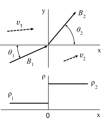
Figure 1: Changes in the magnetic field ${\bf B}$, velocity field ${\bf v}$, and plasma density $\rho$ at the shock front $x=0$. Since $E_{z}\neq 0$ in the coordinate system associated with the current layer, the velocity vectors are not parallel to the magnetic field vectors.

axis (Fig. 1). In the approximation of ideal MHD, we neglect the plasma viscosity, thermal conductivity, and electric resistivity. The boundary conditions for the MHD equations at the discontinuity then take the form of the following conservation laws (Syrovatskii, 1957):

$$\left\{\,B_{x}\,\right\}=0\,,$$ (1)

$$\left\{\,\rho\,v_{x}\,\right\}=0\,,$$ (2)

$$\left\{\,v_{x}B_{y}-v_{y}B_{x}\,\right\}=0\,,$$ (3)

$$\left\{\,v_{x}B_{z}-v_{z}B_{x}\,\right\}=0\,,$$ (4)

$$\left\{\,\rho\,v_{x}v_{y}-\frac{1}{4\pi}\,B_{x}B_{y}\,\right\}=0\,,$$ (5)

$$\left\{\,\rho\,v_{x}v_{z}-\frac{1}{4\pi}\,B_{x}B_{z}\,\right\}=0\,,$$ (6)

$$\left\{\,p+\rho\,v^{\,2}_{x}+\frac{B^{\,2}}{8\pi}\,\right\}=0\,,$$ (7)

$$\left\{\,\rho\,v_{x}\left(\frac{v^{\,2}}{2}+\epsilon+\frac{p}{\rho}\right)+\frac{1}{4\pi}\left(\,B^{\,2}v_{x}-(\,{\bf v}\cdot{\bf B}\,)\,B_{x}\,\right)\right\}=0\,.$$ (8)

Here, the curly brackets denote the difference between the values of the quantity contained within the brackets on both sides of the discontinuity plane. For example, Eq. (1) implies the continuity of the normal magnetic field component:

$$\left\{\,B_{x}\,\right\}=B_{x2}-B_{x1}=0\,.$$

The quantities marked by the subscripts “1” and “2” refer to the side corresponding to the plasma inflow and outflow, respectively.

In contrast to the boundary conditions in ordinary hydrodynamics, the system of boundary conditions (1)–(8) does not break up into a set of mutually exclusive groups of equations and, hence, in principle it admits continuous transitions between different types of discontinuous solutions as the plasma flow conditions change continuously. Since a smooth transition between discontinuities of various types is possible, the local external attributes of the flow near the discontinuity plane are taken as a basis for their classification: the presence or absence of a mass flux and a magnetic flux through the discontinuity, the density continuity or jump.

In the presence of transition solutions, the classification of discontinuities in MHD can only be relative. Indeed, a discontinuity of a given type can continuously pass into a discontinuity of another type as the plasma inflow and magnetic field parameters change gradually. As it will be shown in the Sect. 7 the type of discontinuity can change when passing to a different point of the discontinuity surface. In any case, since a smooth transition is possible between discontinuities of various types, the local external signatures of the flow near the discontinuity plane are taken as a basis for their classification: the presence or absence of velocity, $v_{x}$, and the magnetic field, $B_{x}$, components perpendicular to the plane (i.e., normal), the continuity or jump in density $\rho$. With respect to these signatures, the energy conservation law (8) is an additional condition: at the magnetic field strength, the velocity field, and the density jump found, Eq. (8) defines the jump in pressure $p$. Thus, considering our objective of identifying the discontinuities near the reconnecting current layer in mind, we can restrict our analysis to the remaining seven equations: (1)–(7).

It is necessary to establish conditions under which certain types of discontinuous are formed. Let’s rotate the coordinate system about the $x$ axis in order to make $v_{z1}=0$. The substitution of Eqs. (1)–(2) in (6) will then yield the equation

$${B_{x}\over{4\pi}}\,\{B_{z}\}=\rho v_{x}\,v_{z2}\,.$$ (9)

Here are some simple particular solutions of this equation:

1. If $B_{x}=0$, $v_{x}=0$, i.e., there are no magnetic flux and plasma flow through the discontinuity, then $\{v_{y}\}$, $\{B_{y}\}$, $\{B_{z}\}$ and $\{v_{z2}\}$ are arbitrary quantities as we see from Eqs. (3), (5) and (9). The Eq. (7) implies that the pressure and the magnetic field strength are related by the continuity of the total pressure

   $$\left\{\,p+\frac{B^{\,2}}{8\pi}\,\right\}=0\,,$$

   This solution corresponds to the classical tangential discontinuity.

2. If $B_{x}=0$, $v_{x}\neq 0$ (then from Eq. 9 $v_{z}=0$), the magnetic field is parallel to the discontinuity surface and increases with the compression of the plasma due to a freezing condition, as we see from Eqs. (2), (4).

   $$\left\{\frac{\bf B}{\rho}\right\}=0\,.$$

   This is a perpendicular shock, that is well-known in MHD.

3. If $B_{x}\neq 0$, $v_{x}=0$ (then from Eq. 9 $\{B_{z}\}=0$), $v_{y}$, $v_{z}$ and $B_{y}$ are continuous from Eqs. (3), (5). The direction of the magnetic field does not change, however, the value of the density may change. This is a contact discontinuity.

4. If $B_{x}\neq 0$, $v_{x}\neq 0$, then substitution $v_{z}=0$ in Eq. (9) gives $\{B_{z}\}=0$. As a result, Eq. (4) is transformed into

   $$B_{z}\{v_{x}\}=0\,.$$

   It allows two different solutions:

   1. At the first, we consider the solution $\{v_{x}\}=0$. The substitution of this condition in Eq. (2) gives Alfven wave ($\{\rho\}=0$). Then Eq. (7) rewriting as $\{B_{y}^{2}\}=0$.

   2. Solution $B_{x}=0$ leads us to the two-dimensional picture of the discontinuity: the velocity and the magnetic field lie in the same plane orthogonal to the discontinuity plane.

Thus, the presence or absence of the plasma overflow and penetration of the magnetic field through the discontinuity surface allows identifying all types of discontinuities listed above; for details of their properties see, e.g., Syrovatskii (1956); Somov (2013a). The description of many discontinuities is simplified in the coordinate system, often called the de Hoffmann-Teller system. Such coordinate system moving along the discontinuity plane with velocity

$${\bf u}_{{}_{\,\rm HT}}={\bf v}-\frac{v_{x}}{B_{x}}\,{\bf B}\,,$$

Then the vector ${\bf B}$ becomes parallel to the vector ${\bf v}$. In particular, Alfven discontinuity describes as the rotation of the magnetic field vector around the x axis and all oblique discontinuous (with the magnetic field inclined to the discontinuity plane) become two-dimensional in this case. The de Hoffmann-Teller system is inapplicable to tangential discontinuity and perpendicular shock wave due to the limitation $B_{x}\neq 0$, and we will not use it.

However, taking into account that all discontinuities apart a tangential and an Alfven discontinuity and a perpendicular shock can be reduced to a two-dimensional form, let us begin consideration of the boundary conditions (1)–(8) with the two-dimensional case $4({\rm b})$. We will study only the classification features discontinuous flows to Sect. 6. Therefore, we will not use Eq. (8). Two-dimensional discontinuities will be described by the five boundary conditions:

$$\left\{\,B_{x}\,\right\}=0\,,\quad\,\,\{\rho v_{x}\}=0\,,\quad\,\,\left\{\rho v_{x}v_{y}-{B_{x}B_{y}\over 4\pi}\right\}=0\,,$$ (10)

$$\{v_{x}B_{y}-v_{y}B_{x}\}=0\,,\quad\,\,\left\{\rho v_{x}^{\,2}+p+{B_{y}^{\,2}\over 8\pi}\right\}=0\,.$$

In the next section we will study the change of the magnetic field on the discontinuity surface based on the system (10).

3 Inclination angles

We will write the system of Eqs. (10) in the linear form with respect to the variables $\{v_{x}\}$, $\{v_{y}\}$, $\{r\}$ and $\{B_{y}\}$:

$$\{v_{x}\}-m\,\{r\}=0\,,\quad\,\,m\,\{v_{y}\}-{B_{x}\over 4\pi}\,\{B_{y}\}=0\,,$$

$$\tilde{B}_{y}\{v_{x}\}-B_{x}\{v_{y}\}+m\,{\tilde{r}}\,\{B_{y}\}=0\,,$$ (11)

$$m\,\{v_{x}\}+\{p\}+{\tilde{B}_{y}\over 4\pi}\,\{B_{y}\}=0\,,$$

where we introduced new variables $r=1/\rho$ and $m=\rho v_{x}$. The mean of the two quantities is denoted by the tilde $\tilde{r}~{}=~{}(r_{1}+r_{2})/2$.

For existing nontrivial solutions of the linear system of Eqs. (11), the determinant composed of its coefficients must be equal to zero:

$$\begin{vmatrix}\,-1&0&m&0\\ 0&m&0&-{B_{x}}/{4\pi}\,\,\\ \tilde{B}_{y}&-B_{x}&0&m\tilde{r}\\ m&0&{\{p\}}/{\{r\}}&{\tilde{B}_{y}}/{4\pi}\,\end{vmatrix}=0\,.$$

Let us expand the determinant:

$${\{p\}\over\{r\}}\left({B_{x}^{\,2}\over 4\pi}-m^{\,2}{\tilde{r}}\right)+m^{\,2}\left({B_{x}^{\,2}\over 4\pi}+{\tilde{B}_{y}^{\,2}\over 4\pi}-m^{\,2}{\tilde{r}}\right)=0\,.$$

The latter equation imposes constraints on the admissible values of the mass flux $m$:

$$m^{\,2}=-\,{\{p\}\over\{r\}}\,{{m^{\,2}-{B_{x}^{\,2}}/\,{4\pi\,{\tilde{r}}}}\over{m^{\,2}-\left(B_{x}^{\,2}+\tilde{B}_{y}^{\,2}\right)/\,4\pi\,{\tilde{r}}}}\,.$$ (12)

We can not describe the internal structure of the discontinuity in terms of ideal MHD. Therefore, the discontinuity appears to the surface of zero thickness. However, the irreversible processes in the shock waves leads to the entropy increase. It is essential that the amount of the entropy change does not depend on the specific dissipation mechanism and its jump is determined by the mass, momentum and energy conservation laws (see, e.g., Zel dovich & Raizer, 1967). The entropy increase according to the Zemplen theorem forbids the rarefaction shock waves. Thus,

$$\{r\}=\frac{1}{\rho_{2}}-\frac{1}{\rho_{1}}=\frac{\rho_{1}-\rho_{2}}{\rho_{1}\rho_{2}}<0\,.$$

The quantity $m^{2}$ can not be negative. Therefore, two inequalities must hold: either

$$m^{\,2}<{B_{x}^{\,2}\over 4\pi\,{\tilde{r}}}\,,$$ (13)

or

$$m^{\,2}>{{B_{x}^{\,2}+\tilde{B}_{y}^{\,2}}\over{4\pi\,{\tilde{r}}}}\,.$$ (14)

The solution of the system of Eqs. (11) is

$$\{v_{x}\}=C\,m\left({B_{x}^{\,2}\over 4\pi}-m^{\,2}{\tilde{r}}\right)\,,$$

$$\{v_{y}\}=C\,m{B_{x}\tilde{B}_{y}\over 4\pi}\,,$$ (15)

$$\{r\}=C\left({B_{x}^{\,2}\over 4\pi}-m^{\,2}{\tilde{r}}\right)\,,$$

$$\{B_{y}\}=C\,m^{\,2}\tilde{B}_{y}\,,$$

We find the constant $C$ by substituting the expressions for $\{v_{x}\}$ and $\{B_{y}\}$ for the last equation of the system (11):

$$C=-\,{\{p\}\over m^{\,2}}\left({B_{x}^{\,2}+\tilde{B}_{y}^{\,2}\over 4\pi}-m^{\,2}\tilde{r}\right)^{\!-1}.$$

Consider the last two equations of the system (15). Eliminating the constant $C$ from them, we will obtain the relationship between the tangential magnetic field components

$$\{B_{y}\}={m^{\,2}\{r\}\over\left({B_{x}^{\,2}}/\,{4\pi}-m^{\,2}{\tilde{r}}\right)}\,\tilde{B}_{y}\,.$$

Expanding the relations

$$\{B_{y}\}=B_{y2}-B_{y1}$$

and

$$\tilde{B}_{y}={1\over 2}(B_{y2}+B_{y1})\,,$$

we then have

$$B_{y2}={2\left({B_{x}^{\,2}}/\,{4\pi}-m^{\,2}{\tilde{r}}\right)+m^{\,2}\{r\}\over 2\left({B_{x}^{\,2}}/\,{4\pi}-m^{\,2}{\tilde{r}}\right)-m^{\,2}\{r\}}\,B_{y1}\,.$$ (16)

Let us divide both parts of Eq. (16) by $B_{x}$ to obtain the relation of the angles between the magnetic field vector and the normal to the discontinuity surface on both its sides:

$${\rm tan}\,\theta_{2}={2\,\left(\,{B_{x}^{\,2}}/\,{4\pi}-m^{\,2}\,{\tilde{r}}\,\right)+m^{\,2}\,\{\,r\,\}\over 2\,\left(\,{B_{x}^{\,2}}/\,{4\pi}-m^{\,2}\,{\tilde{r}}\,\right)-m^{\,2}\,\{\,r\,\}}\,\,{\rm tan}\,\theta_{1}\,.$$

Here, ${\rm tan}\,\theta=B_{y}/\,B_{x}$, $r=1/\rho\,$, and the tilde marks the mean values of the quantities, $\tilde{r}=(\,r_{1}+r_{2}\,)/\,2$. Rewriting this formula by expanding the jumps $\{r\}$ and the means $\tilde{r}$, we obtain

$${\rm tan}\,\theta_{2}={m^{\,2}\cdot 4\pi r_{1}/B_{x}^{\,2}-1\over m^{\,2}\cdot 4\pi r_{2}/B_{x}^{\,2}-1}\,\,{\rm tan}\,\theta_{1}\,.$$

Denote $m_{\rm off}^{\,2}=B_{x}^{\,2}/4\pi r_{1}$ and $m_{\rm on}^{\,2}=B_{x}^{\,2}/4\pi r_{2\,}$; as will be shown below, $m_{\rm off}$ and $m_{\rm on}$ correspond to the mass flux through the switch-off and switch-on shocks. Note that $m_{\rm off}~{}\leq~{}m_{\rm on}$, because according to Zemplen s theorem, $r_{2}\leq r_{1}$. The formula for the field inclination angles takes form

$${\rm tan}\,\theta_{2}=\frac{m^{2}/m_{\rm off}^{2}-1}{m^{2}/m_{\rm on}^{2}-1}\,{\rm tan}\,\theta_{1}\,.$$ (17)

Let us denote $m_{{}_{\rm A}}^{\,2}=B_{x}^{\,2}/4\pi{\tilde{r}}$ and $m^{\,2}_{\bot}=\tilde{B}_{y}^{\,2}/\,4\pi{\tilde{r}}$. Since $r_{2}\leq\tilde{r}\leq r_{1}$, $m_{\rm off}\leq~{}m_{{}_{\rm A}}\leq m_{\rm on}$. Then we will write conditions (13) and (14) as:

$$m^{\,2}<m_{{}_{\rm A}}^{\,2}\,,$$ (18)

$$m^{\,2}>m_{{}_{\rm A}}^{\,2}+m_{\bot}^{\,2}\,.$$ (19)

Note that $m_{\rm off}$, $m_{\rm A}$ and $m_{\rm on}$ are not independent but are related by the equation

$$m_{{}_{\rm A}}^{\,2}=\frac{2\,\,m_{\rm on}^{\,2}\,m_{\rm off}^{\,2}}{m_{\rm on}^{\,2}+m_{\rm off}^{\,2}}\,.$$ (20)

This can be easily verified by expanding the mean $\tilde{r}$ in the definition of $m_{\rm A}^{\,2}$.

Based on these results we will consider the properties of discontinuous flows; more specifically, we will establish the possible transitions between them.

4 Transition solutions

We begin to seek transition solutions with a search for the conditions of possible transitions between various types of two-dimensional MHD flows ($v_{z}=0$, $B_{z}=0$), i.e., flows for which the velocity field and the magnetic field lie in the $(x,y)$ plane. We call such discontinuous flows plane or two-dimensional ones. Then, we will find the transition solutions that correspond to them and establish the form of the solutions that are the transition ones to three-dimensional discontinuous flows.

Equation (17) along with conditions (18)–(19) describes the dependence of the magnetic field inclination angles on the mass flux through the discontinuity. This dependence can be specified either by the two parameters $m_{\rm off}$ and $m_{\rm on}$, or, for example, by the quantities $\rho_{1}$ and $\{\rho\}$. Since we are interested in the classification attributes of discontinuities (i.e., the qualitative changes of the relation between the angles $\theta_{1}$ and $\theta_{2}$ when varying $m^{2}$), for the time being, we will consider Eq. (17) without any specific application to certain physical conditions in the plasma. We will choose the parameters from clarity considerations. Let $m_{\rm off}^{\,2}$, $m_{{}_{\rm A}}^{\,2}$ and $m_{\rm on}^{\,2}$ be related as $3:4:6$. We will measure the square of the mass flux in units of $m_{{}_{\rm A}}^{\,2}/4$; then $m_{\rm off}^{\,2}=3$ and $m_{\rm on}^{\,2}=6$. The dependence $\theta_{2}(m^{2})$ is shown in Fig. 2

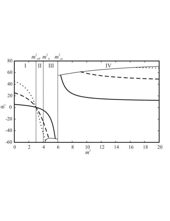
Figure 2: Inclination angle of the magnetic field $\theta_{2}$ behind the discontinuity plane versus the square of the mass flux $m^{2}$ at various angles $\theta_{1}$ . The cases of $\theta_{1}=1^{\circ}$, $\theta_{1}=25^{\circ}$, $\theta_{1}=45^{\circ}$ are designated by the solid, dashed, and dotted lines, respectively.

or three values of the angle $\theta_{1}$. The corresponding curves behave identically. Firstly, they intersect at one point at $m^{2}=m_{\rm off}^{\,2}$, $\theta_{2}=0$ here. Secondly, $\theta_{2}\rightarrow-\,\theta_{1}$ when $m^{2}\rightarrow m_{{}_{\rm A}}^{\,2}=4$. for each curve. Thirdly, they all have a region that does not satisfy conditions (18) and (19), located near $m^{2}=m_{\rm on}^{\,2}$.

Let us separate out the regions in Fig. 2 each of which is characterized by its own behavior of the dependence of $\theta_{2}$ on $m^{2}$. In region ${\rm I}$ ($0<m^{2}<m_{\rm off}^{\,2}$), the tangential component $B_{y2}$ of the magnetic field vector ${\bf B}_{2}$ behind the discontinuity surface decreases with increasing $m^{2}$. In this case, $0<\theta_{2}<\theta_{1}$, i.e., when passing through the discontinuity surface, the tangential field component weakens but remains positive. At $m^{2}=m_{\rm off}^{\,2}$ when crossing the discontinuity plane, $B_{y2}$ becomes zero. In region ${\rm II}$ ($m_{\rm off}^{\,2}<m^{2}<m_{{}_{\rm A}}^{\,2}$) $B_{y2}$ is negative and increases in magnitude, but $-\theta_{1}<\theta_{2}<0$. In region ${\rm III}$ ($m_{{}_{\rm A}}^{\,2}<m^{2}<m_{\rm on}^{\,2}$), just as in region ${\rm II}$, $B_{y}$ changes its sign when crossing the discontinuity plane. Now, however, $B_{y}$ increases in magnitude ($\theta_{2}<-\theta_{1}$), remaining negative. Finally, in region ${\rm IV}$ ($m^{2}>m_{\rm on}^{\,2}$) the magnetic field is amplified ($\theta_{2}>\theta_{1}$) with its tangential component retaining the positive sign.

Thus, we have shown precisely how the behavior of the relation between the magnetic field inclination angles and, consequently, the type of MHD discontinuity changes with the increasing mass flux. The regions I and II correspond to the slow shocks that, respectively, do not reverse ($S_{-}^{\,\uparrow}$) and reverse (${S_{-}^{\,\downarrow}}$) the tangential field component. The regions III and IV correspond to the trans-Alfven (${Tr}$) and fast (${S_{+}}$) shocks, respectively. Shock waves corresponding to the regions II and III is often called intermediate shocks (Sterck et al., 1998). The plasma velocity is super-Alfven upstream, and sub-Alfven downstream at the intermediate shocks while the slow shocks is everywhere sub-Alfven and fast shocks is everywhere super-Alfven. We use the mass flux as a classifier rather than the plasma velocity. This classifier divides the intermediate shocks into two types which have the different properties. Therefore, we will use different names for the discontinuities in the regions II and III. The transition solutions for the discontinuities corresponding to the adjacent regions are realized at the mass flux demarcating these regions.

Consider the behavior of the function $\theta_{2}(m^{2},\theta_{1})$ near the boundary of regions ${\rm II}$ and ${\rm III}$, where $m^{\,2}=m_{{}_{\rm A}}^{\,2}$. The domain of definition of the function $\theta_{2}(m^{2},\theta_{1})$ to the left and the right of $m_{{}_{\rm A}}^{\,2}$ is specified by conditions (18), and (19), respectively. In view of Eqs. (17) and (20), ${\rm tan}\,\theta_{2}\to-{\rm tan}\,\theta_{1}$ when $m^{\,2}\to m_{{}_{\rm A}}^{\,2}$, i.e., $\tilde{B}_{y}\to 0$. Inequality (19) transforms to $m^{\,2}>m_{{}_{\rm A}}^{\,2}$. in this case. Therefore, the function $\theta_{2}(m^{2},\theta_{1})$ in region ${\rm II}$ and region ${\rm III}$ is defined near $m_{{}_{\rm A}}^{\,2}$. However, the right part of the condition $m^{2}$ also increases with (19). The equality $m^{2}=m_{{}_{\rm A}}^{\,2}+m_{\bot}^{\,2}$ is established at some value of $m^{2}$ in region ${\rm III}$ and the strongest trans-Alfven shock (increasing the magnetic energy to the greatest extent) takes place. As the mass flux increases further, $m^{2}$ can not satisfy conditions (18) and (19) until $m^{2}$ again becomes equal to $m_{{}_{\rm A}}^{\,2}+m_{\bot}^{\,2}$. This occurs in region ${\rm IV}$, where the strongest fast shock is observed.

Let us derive the equation of the curve bounding the function $\theta_{2}(m^{2},\theta_{1})$, and, hence, the strongest (for given plasma parameters), fast and trans-Alfven shocks. Setting $m^{\,2}$ equal to the right part of condition (14), we find

$$B_{y1}=\pm\,2\,\sqrt{4\pi\tilde{r}\,m^{2}-B_{x}^{2}}\,-B_{y2}\,,$$

where the plus and minus correspond to regions IV and III, respectively. Dividing the derived equation by $B_{x}$, we have

$${\rm tan}\,\theta_{1}=\pm\,2\,\sqrt{m^{2}/\,m_{{}_{\rm A}}^{\,2}-1}\,-{\rm tan}\,\theta_{2}\,.$$ (21)

Substituting Eq. (21) in (17), we obtain the equation of the sought-for curve

$${\rm tan}\,\theta_{2}=\pm\,\frac{m^{\,2}/\,m_{\rm off}^{\,2}-1}{\sqrt{m^{\,2}/\,m_{\rm A}^{\,2}-1}}\,.$$ (22)

The corresponding curves are represented in Fig. 2 by the thin lines.

Now, we will seek transition solutions in order of the increasing mass flux $m$, starting from $m=0$. Let’s consider the transition between the contact discontinuity (${C}$) at $m^{2}=0$ and the slow shock in region I. The boundary conditions for two-dimensional discontinuities follow from Eqs. (1)–(7) when $v_{z}=0$ and $B_{z}=0$ are substituted:

$$\left\{\,B_{x}\,\right\}=0\,,\quad\left\{\,\rho\,v_{x}\,\right\}=0\,,\quad\left\{\,p+\rho\,v^{\,2}_{x}+\frac{B_{y}^{\,2}}{8\pi}\,\right\}=0\,,$$ (23)

$$\left\{\,v_{x}B_{y}-v_{y}B_{x}\,\right\}=0\,,\quad\left\{\,\rho\,v_{x}v_{y}-\frac{1}{4\pi}\,B_{x}B_{y}\,\right\}=0\,.$$

The solution of these equations in region I presented in Fig. 2 corresponds to the slow shock ($S_{-}^{\,\uparrow}$) that does not change the sign of the tangential magnetic field component. This can be easily verified at small $m^{2}$. It follows from Eq. (17) which, of course, remains applicable under conditions of the two-dimensional discontinuous flows that

$${\rm tan}\,\theta_{2}\approx\left(1-\frac{m^{2}}{m_{\rm off}^{2}}+\frac{m^{2}}{m_{\rm on}^{2}}\right)\,{\rm tan}\,\theta_{1}\,,$$

i.e., $0<\theta_{2}<\theta_{1}$, as it must be in the slow shock. Moreover, when $m^{2}\rightarrow 0$, i.e., $v_{x}\rightarrow 0$, it follows from the system (23) that $\left\{\,v_{y}\,\right\}\rightarrow 0$ and $\left\{\,B_{y}\,\right\}\rightarrow 0$ which is the only limiting case for the slow shock.

It remains to show that when $v_{x}\rightarrow 0$, conditions (23) transform to the boundary conditions at the contact discontinuity. Indeed, the substitution of $v_{x}=0$ in (23) gives

$$\left\{\,B_{x}\,\right\}=\left\{\,v_{y}\,\right\}=\left\{\,B_{y}\,\right\}=\left\{\,p\,\right\}=0\,,$$ (24)

At the contact discontinuity, the jump in density $\{\rho\}$ is nonzero. Otherwise, all quantities remain continuous. Thus, solution (24) simultaneously describes the slow shock in the limit $v_{x}\rightarrow 0$,and the contact discontinuity, i.e., it is the corresponding transition solution.

When crossing the boundary of regions I and II, the tangential magnetic field component changes its sign. The slow shock ($S_{-}^{\,\uparrow}$) that does not reverse the tangential field component turns into the reversing slow shock (${S_{-}^{\,\downarrow}}$). The transition solution is realized on the boundary of the regions, when $\theta_{2}=0$. The substitution of $B_{y2}=0$ in (23) gives the corresponding transition solution:

$$\left\{\,B_{x}\,\right\}=0\,,\quad\left\{\,\rho\,v_{x}\,\right\}=0\,,\quad\left\{\,p+\rho\,v^{\,2}_{x}\,\right\}=\frac{B_{y1}^{\,2}}{8\pi}\,,$$ (25)

$$B_{x}\left\{\,v_{y}\,\right\}=-v_{x1}B_{y1}\,,\quad\rho\,v_{x}\left\{\,v_{y}\,\right\}=-\frac{1}{4\pi}\,B_{x}B_{y1}\,.$$

Eliminating $\{v_{y}\}$ from the last two equations, we find

$$m^{2}={\rho_{1}B_{x}^{\,2}}/\,{4\pi}=m_{\rm off}^{\,2}\,,$$ (26)

which was to be proved. This mass flux corresponds to the switch-off shock (${S_{\,\rm off}}$): the tangential field component disappears behind the discontinuity plane. This occurs irrespective of the angle $\theta_{1}$ and corresponds to the intersection of the curves at $m^{2}=m_{\rm off}^{\,2}$ in Fig. 2.

The reversal of the tangential field component at the boundary of regions II and III can be a special case of the three-dimensional Alfven discontinuity (${A}$). Since there is no density jump at the Alfven discontinuity, let us substitute $\{\rho\}=0$ in (23):

$$\left\{\,\rho\,\right\}=\left\{\,B_{x}\,\right\}=\left\{\,v_{x}\,\right\}=0\,,\quad\left\{\,p+\frac{B_{y}^{\,2}}{8\pi}\,\right\}=0\,,$$ (27)

$$B_{x}\left\{\,v_{y}\,\right\}=v_{x}\left\{\,B_{y}\,\right\}\,,\quad\rho\,v_{x}\left\{\,v_{y}\,\right\}=\frac{1}{4\pi}\,B_{x}\left\{\,B_{y}\,\right\}\,.$$

If $\{B_{y}\}=0$, then all quantities are continuous and there is no discontinuity. Let $\{B_{y}\}\neq 0$. Eliminating the ratio $\{B_{y}\}/\{v_{y}\}$ from the last two equations, we obtain

$$m^{\,2}={\rho B_{x}^{\,2}}/\,{4\pi}=m_{{}_{\rm A}}^{\,2}\,.$$ (28)

When substituting $\{\rho\}=0$ in (1)–(7), we find the boundary conditions at the Alfven discontinuity:

$$\left\{\,\rho\,\right\}=\left\{\,B_{x}\,\right\}=\left\{\,v_{x}\,\right\}=0\,,\quad\left\{\,p+\frac{B_{y}^{\,2}+B_{z}^{\,2}}{8\,\pi}\,\right\}=0\,,$$ (29)

$$B_{x}\left\{\,v_{y}\,\right\}=v_{x}\left\{\,B_{y}\,\right\}\,,\quad\rho\,v_{x}\,\left\{\,v_{y}\,\right\}=\frac{1}{4\pi}\,B_{x}\left\{\,B_{y}\,\right\}\,,$$

$$B_{x}\left\{\,v_{z}\,\right\}=v_{x}\left\{\,B_{z}\,\right\}\,,\quad\rho\,v_{x}\,\left\{\,v_{z}\,\right\}=\frac{1}{4\pi}\,B_{x}\left\{\,B_{z}\,\right\}\,.$$

Comparison of the systems (27) and (29) shows that the boundary conditions (27) describe the transition discontinuity between the slow shock in the limit $\{\rho\}\rightarrow 0$ and the Alfven flow at $v_{z}=0$ and $B_{z}=0$. The discontinuity is a special case of the Alfven discontinuity that reverses the tangential magnetic field component. Trans-Alfven discontinuities reverse and enhance the tangential field component. They occupy region III and are adjacent to the Alfven mass flux (28) on the right side. The conditions for the transition to the Alfven discontinuity are identical to (27).

There can be no flow near the boundary of regions III and IV in some range of mass fluxes. For this reason, the transition between the trans-Alfven and fast shock is forbidden. The range narrows as the initial inclination angle of the magnetic field decreases to $\theta_{1}=0$ (Fig. 3).

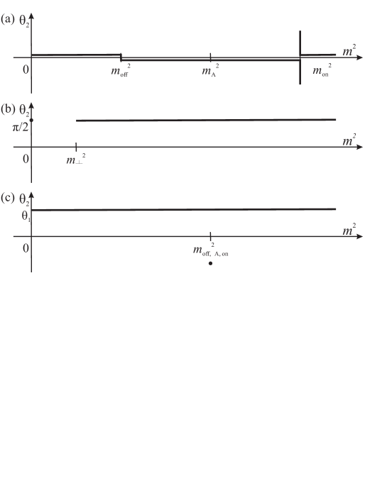
Figure 3: Schematic behavior of the dependence $\theta_{2}(m^{2})$ at $\theta_{1}=0$ (a), $B_{x}=0$ (b), and $\{\rho\}=0$ (c).

The strongest fast shock takes place at the minimum possible mass flux that is admissible by condition (19). As the mass flux increases, the tangent of the field inclination angle behind the discontinuity plane decreases, asymptotically approaching ${\rm tan}\,\theta_{2}=({\rho_{2}/\rho_{1}})\,{\rm tan}\,\theta_{1}$.

5 The scheme of transitions

Varying $\rho_{1}$, $\{\rho\}$ and $B_{x}$ leads to contraction or extension of the curves presented in Fig. 2 along the coordinate axes without any change of their overall structure. For zero $\theta_{1}$, $B_{x}$ and $\{\rho\}$ the behavior of dependence $\theta_{2}(m^{2})$ is shown in Fig. 3. In view of Eq. (17) when $\theta_{1}\rightarrow 0$, the angle $\theta_{2}$ also approaches zero at almost all values of $m^{2}$ (the case of $m^{2}=m_{\rm on}^{\,2}$ will be considered separately). If $B_{y1}=0$, then $B_{y2}=0$ (Fig. 3a). In this case, the boundary conditions for the two-dimensional discontinuities (10) take the form

$$\left\{\,\rho\,v_{x}\,\right\}=0\,,\quad\left\{\,p+\rho\,v^{2}_{x}\,\right\}=0\,,$$ (30)

$$\left\{\,B_{x}\,\right\}=0\,,\quad\left\{\,v_{y}\,\right\}=0\,,$$

which corresponds to an ordinary hydrodynamic shock that propagates according to the conditions $B_{y1}=0$ and $B_{y2}=0$ along the magnetic field. System (30) is the transition solution between the oblique shocks in the limit $\theta_{1}\rightarrow 0$ and the parallel shock (${S_{\parallel}}$).

As the angle $\theta_{1}$ decreases, the discontinuity between the admissible mass fluxes for the fast and the trans-Alfven shocks will also decrease. Conditions (10) in this case give

$$\left\{\,B_{x}\,\right\}=0\,,\quad\left\{\,\rho\,v_{x}\,\right\}=0\,,\quad\left\{\,p+\rho\,v^{\,2}_{x}\,\right\}=-\frac{B_{y2}^{\,2}}{8\pi}\,,$$ (31)

$$B_{x}\left\{\,v_{y}\,\right\}=v_{x2}B_{y2}\,,\quad\rho\,v_{x}\left\{\,v_{y}\,\right\}=\frac{1}{4\pi}\,B_{x}B_{y2}\,.$$

From the simultaneous solution of the last two equations, we have

$$m^{2}={\rho_{2}B_{x}^{\,2}/\,4\pi}=m_{\rm on}^{\,2}.$$ (32)

For this mass flux, Eq. (17) has no unique solution. A nonzero $\theta_{1}$ can correspond to zero $\theta_{2}$. The tangential magnetic field component appears behind the shock front, corresponding to the switch-on shock (${S_{\,\rm{on}}}$). It is indicated in Fig. 3a by the vertical segment at $m^{2}=m^{2}_{\,\rm{on}}$. The switch-on shock can act as the transition one for the trans-Alfven and fast shocks in the limit $\theta_{1}\rightarrow 0$, but this, of course, requires that $m^{2}\rightarrow m^{2}_{\,\rm{on}}$. Otherwise, there will be the transition to the parallel shock according to (30).

To establish the form of the transition solution between the parallel shock and the contact discontinuity, we will set $v_{x}=0$ in (30). After that we will obtain

$$\left\{\,B_{x}\,\right\}=\left\{\,v_{y}\,\right\}=\left\{\,p\,\right\}=0\,,$$ (33)

This system of equations corresponds to the contact discontinuity (24), orthogonal to the magnetic field lines. It describes the transition discontinuity between the parallel shock in the limit $v_{x}\rightarrow 0$ and the contact discontinuity. Such a transition takes place at $m^{2}=0$ in Fig. 3a.

When $B_{x}=0$ (Fig. 3b), $m^{2}_{\,\rm{on}}$ becomes zero and all nonzero mass fluxes locate in region IV in Fig. 2. To find the boundary conditions corresponding to them, let us substitute $B_{x}=0$ in (10). We obtain

$$\left\{\,\rho\,v_{x}\,\right\}=0\,,\quad\left\{\,p+\rho\,v^{\,2}_{x}+\frac{B_{y}^{\,2}}{8\pi}\right\}=0\,,$$ (34)

$$\left\{\,v_{x}B_{y}\,\right\}=0\,,\quad\left\{\,v_{y}\,\right\}=0\,.$$

These conditions characterize a compression shock propagating perpendicularly to the magnetic field. In the general case of a perpendicular shock (${S_{\bot}}$) we will find the boundary conditions by substituting $B_{x}=0$ in (1)–(7):

$$\left\{\,\rho\,v_{x}\,\right\}=0\,,\quad\left\{\,p+\rho\,v^{\,2}_{x}+\frac{B_{y}^{\,2}+B_{z}^{\,2}}{8\pi}\,\right\}=0\,,$$

$$\left\{\,v_{x}B_{y}\,\right\}=0\,,\quad\left\{\,v_{y}\,\right\}=0\,,$$ (35)

$$\left\{\,v_{x}B_{z}\,\right\}=0\,,\quad\left\{\,v_{z}\,\right\}=0\,.$$

Equations (34) are then the boundary conditions for the transition discontinuity between the fast shock in the limit $B_{x}\rightarrow 0$ and the perpendicular shock with the magnetic field directed along the $y$-axis. This transition can take place only at mass fluxes that satisfy inequality (19) which takes the form $m^{\,2}>m^{\,2}_{\bot}$ at $B_{x}=0$ (Fig. 3b).

To determine the boundary conditions for the discontinuity at $m^{2}=0$ (Fig. 3c), let us substitute $B_{x}=0$ and $v_{x}=0$ in (1)–(7). In this case, the magnetic field and the velocity field are parallel to the discontinuity surface and can undergo arbitrary jumps in magnitude and direction, while the jump in pressure is related to the jump in the magnetic field by the condition

$$\left\{\,p+\frac{B_{y}^{\,2}+B_{z}^{\,2}}{8\pi}\,\right\}=0\,.$$ (36)

This corresponds to the tangential discontinuity (${T}$). The contact discontinuity, the slow shock, and the Alfven discontinuity can pass to it in the limit $B_{x}\rightarrow 0$ under certain conditions. Let us find the corresponding transition solutions. Firstly, let us substitute $B_{x}=0$ in the boundary conditions for the contact discontinuity (24). We will obtain the transition solution

$$\left\{\,B_{y}\,\right\}=\left\{\,v_{y}\,\right\}=\left\{\,p\,\right\}=0\,.$$ (37)

It describes the tangential discontinuity (36) for the zero field component $B_{z}$ in the absence of jumps $\{v_{y}\}$ and $\{B_{y}\}$. Secondly, the conditions for the oblique shocks (10) at $B_{x}=0$ and $v_{x}=0$ are the transition solution

$$\left\{\,p+\frac{B_{y}^{\,2}}{8\pi}\,\right\}=0\,,$$ (38)

that corresponds to the plane tangential discontinuity (36) at $B_{z}=0$. Finally, the boundary condition for the Alfven discontinuity (29) after the substitution of $B_{x}=0$ gives the transition solution

$$\left\{\,\rho\,\right\}=0\,,\quad\left\{\,p+\frac{B_{y}^{\,2}+B_{z}^{\,2}}{8\pi}\,\right\}=0\,,$$ (39)

that describes the tangential discontinuity (36), with out any jump in density $\rho$.

The angle $\theta_{2}$ of the strongest trans-Alfven shock is defined by Eq. (21). In view of (21), $\theta_{2}\rightarrow-\theta_{1}$ when $B_{x}\rightarrow 0$. Thus, the trans-Alfven shocks degenerate into a special case of the Alfven discontinuity as the magnetic flux decreases. Of course, the density jump can also be set equal to zero for any type of flow. In this case, all parameters $m^{2}_{\,\rm{off}}$, $m_{{}_{\rm{A}}}^{\,2}$ and $m^{2}_{\,\rm{on}}$ will be equal to the flux (28), at which the Alfven discontinuity (27) takes place. In Fig. 3c, it is denoted by $m^{2}_{\,\rm{off,A,on}}$. At other mass fluxes, the differences in plasma characteristics on different sides of the discontinuity will disappear; the discontinuity will be absent as such.

Let us combine the properties of discontinuous solutions systematized above into the scheme of permitted transitions shown in Fig. 4.

Figure 4: Scheme of continuous transitions between MHD discontinuities. The dashed line encircles the set of discontinuities corresponding to the block of oblique shocks in the scheme by Syrovatskii (1956). The shading inside the contour highlights the slow (left) and fast (right) components of the scheme proposed by Somov (1994).

Here, the two-dimensional discontinuities are located in the middle row in order of increasing the mass flux and the three-dimensional discontinuities are located in the upper row. The one-dimensional parallel shock ($S_{\,\parallel}$) occupies the lower row.

The first description of transition solutions (Syrovatskii, 1956) contained only four types of discontinuous flows: a tangential discontinuity ($T$) and Alfven ($A$), oblique ($S$) and perpendicular ($S_{\bot}$) shocks (Fig. 5).

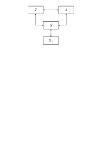
Figure 5: Scheme of continuous transitions between MHD discontinuities (Syrovatskii, 1956)

The corresponding scheme of continuous transitions between discontinuous solutions of the equations of ideal MHD showed such transitions to be possible in principle, but it was definitely incomplete. Firstly, it did not have some of the discontinuous solutions, in particular, the parallel shock ($S_{\,\|}$) and the contact discontinuity ($C$). Secondly, the block of oblique shocks ($S$) combined several different discontinuities at once: fast ($S_{+}$) and slow ($S_{-}$) shocks, switch-on ($S_{\,\rm on}$) and switch-off  ($S_{\,\rm off}$), shocks, and trans-Alfven ($Tr$), shocks, the possibility of transitions between which requires a separate consideration. Subsequently, this picture of transitions was supplemented based on the correspondence between the shocks and small amplitude waves (Somov, 1994).

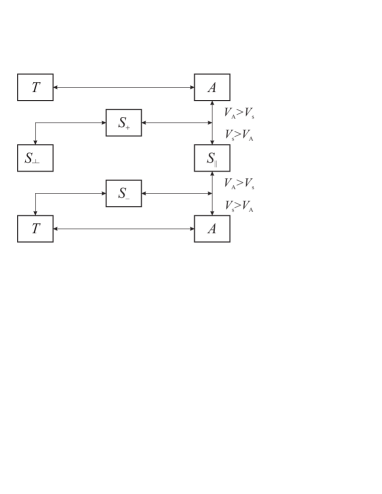
Figure 6: Scheme of continuous transitions between MHD discontinuities (Somov, 1994)

Although this approach allows the possible transitions (Fig. 6) and even their conditions to be correctly specified, it provides no description of the specific form of transition solutions between the discontinuities under consideration.

We group individual elements for the convenience of comparing the generalized scheme of transitions with those proposed previously. Syrovatskii s scheme (Syrovatskii, 1956) is consistent with Fig. 4 if we combine the elements ${S_{-}^{\,\downarrow}}$, ${S_{\,\rm{off}}}$, ${S_{-}^{\,\uparrow}}$, ${Tr}$, ${S_{\,\rm{on}}}$ and ${S_{+}}$ into one block of “oblique shocks” (${S}$), while omitting the question of whether any transitions inside the block are possible and disregard the contact discontinuity (${C}$) and the parallel shock (${S_{\,\parallel}}$). The scheme proposed in (Somov, 1994), includes the parallel shock (${S_{\,\parallel}}$) and the separation of oblique shocks into the slow one (${S_{-}}$), corresponding to condition (18), and the fast one (${S_{+}}$) corresponding to condition (19). It is quite obvious that the scheme of transitions we propose is a proper and natural generalization of the two previous schemes. Our scheme contains not only evolutionary types of discontinuities but also non-evolutionary ones: the switch-on, Alfven, and trans-Alfven shocks.

6 Jump in internal energy

To determine the plasma heating efficiency, let us turn to the boundary condition (8), which is the energy conservation law (Ledentsov & Somov, 2013). Using Eq. (2), we will find the jump in internal energy from (8)

$$\left\{\,\epsilon\,\right\}=-\left\{\frac{v^{\,2}}{2}\right\}-\frac{1}{m}\left\{\,v_{x}p\,\right\}-\frac{1}{4\pi m}\left\{\,B^{\,2}v_{x}-(\,{\bf v}\cdot{\bf B}\,)\,B_{x}\,\right\}.$$ (40)

Using the mean velocities $\tilde{v}_{x}$, $\tilde{v}_{y}$ and $\tilde{v}_{z}$, we will write the first term as

$$-\left\{\frac{v^{\,2}}{2}\right\}=-\tilde{v}_{x}\left\{v_{x}\right\}-\tilde{v}_{y}\left\{v_{y}\right\}-\tilde{v}_{z}\left\{v_{z}\right\}.$$

We will express the jumps in tangential velocity components in terms of the jumps in tangential magnetic field components using Eqs. (1), (2), (5) and (6) as

$$\left\{v_{y}\right\}=\frac{B_{x}}{4\pi m}\left\{B_{y}\right\},\quad\left\{v_{z}\right\}=\frac{B_{x}}{4\pi m}\left\{B_{z}\right\}.$$

Now, the first term on the right side of Eq. (40) appears as

$$-\left\{\frac{v^{\,2}}{2}\right\}=-\tilde{v}_{x}\left\{v_{x}\right\}-\frac{\tilde{v}_{y}B_{x}}{4\pi m}\,\{B_{y}\}-\frac{\tilde{v}_{z}B_{x}}{4\pi m}\,\{B_{z}\}.$$ (41)

Let us substitute in the second term written as

$$-\frac{1}{m}\left\{v_{x}p\right\}=-\frac{\tilde{p}}{m}\{v_{x}\}-\frac{\tilde{v}_{x}}{m}\{p\},$$

the pressure jump from Eq. (7), namely

$$\left\{p\right\}=-m\{v_{x}\}-\frac{\tilde{B}_{y}}{4\pi}\,\{B_{y}\}-\frac{\tilde{B}_{z}}{4\pi}\,\{B_{z}\}.$$

Here, as in Eq. (40), we made use of condition (2). As the result, the second term in Eq. (40) takes on the form

$$-\frac{1}{m}\left\{v_{x}p\right\}=-\frac{\tilde{p}}{m}\,\{v_{x}\}+\tilde{v}_{x}\{v_{x}\}+\frac{\tilde{v}_{x}\tilde{B}_{y}}{4\pi m}\,\{B_{y}\}+\frac{\tilde{v}_{x}\tilde{B}_{z}}{4\pi m}\,\{B_{z}\}.$$ (42)

Let us now open the scalar product $(\,{\bf v}\cdot{\bf B}\,)$ in the third term:

$$-\frac{1}{4\pi m}\left\{\,B^{\,2}v_{x}-(\,{\bf v}\cdot{\bf B}\,)\,B_{x}\,\right\}=$$

$$-\frac{1}{4\pi m}\left\{(v_{x}B_{y}-v_{y}B_{x})B_{y}+(v_{x}B_{z}-v_{z}B_{x})B_{z}\right\}.$$

Then, let us apply conditions Eq. (3) and Eq. (4) to the derived equation:

$$-\frac{1}{4\pi m}\left\{\,B^{\,2}v_{x}-(\,{\bf v}\cdot{\bf B}\,)\,B_{x}\,\right\}=$$

$$-\frac{v_{x}B_{y}-v_{y}B_{x}}{4\pi m}\,\{B_{y}\}-\frac{v_{x}B_{z}-v_{z}B_{x}}{4\pi m}\,\{B_{z}\}.$$ (43)

Thus, each of the three terms in the right side of Eq. (40) is expressed via individual jumps of the normal velocity components and tangential magnetic field components. Let us substitute Eqs. (41)–(43) in (40)

$$\left\{\,\epsilon\,\right\}=-\frac{\tilde{p}}{m}\,\{v_{x}\}+\frac{\tilde{v}_{x}\tilde{B}_{y}-\tilde{v}_{y}B_{x}}{4\pi m}\,\{B_{y}\}-\frac{v_{x}B_{y}-v_{y}B_{x}}{4\pi m}\,\{B_{y}\}\,+$$

$$+\,\frac{\tilde{v}_{x}\tilde{B}_{z}-\tilde{v}_{z}B_{x}}{4\pi m}\,\{B_{z}\}-\frac{v_{x}B_{z}-v_{z}B_{x}}{4\pi m}\,\{B_{z}\}.$$

This equation can be simplified if we expand the means appearing in it:

$$\left\{\,\epsilon\,\right\}=-\frac{\tilde{p}}{m}\,\{v_{x}\}-\frac{\{v_{x}\}\{B_{y}\}}{16\pi m}\,\{B_{y}\}-\frac{\{v_{x}\}\{B_{z}\}}{16\pi m}\,\{B_{z}\}.$$

Factoring out $-\{v_{x}\}/m=-\{r\}$, we derive the final equation, which expresses the internal energy jump at the discontinuity through the jumps of the inverse density and tangential magnetic field components

$$\left\{\,\epsilon\,\right\}=-\{r\}\left(\tilde{p}+\frac{\{B_{y}\}^{2}+\{B_{z}\}^{2}}{16\pi}\right).$$ (44)

For two-dimensional discontinuities, it takes quite a simple form,

$$\left\{\,\epsilon\,\right\}=-\{r\}\left(\tilde{p}+\frac{\{B_{y}\}^{2}}{16\pi}\right).$$ (45)

Equation (44) allows definitive conclusions regarding the change in plasma internal energy when crossing the discontinuity surface to be reached. First, the internal energy increases, because, according to Zemplen s theorem, $-\{r\}>0$ and $\tilde{p}$ and $\{B_{y}\}^{2}$ are positive. Second, the change in internal energy consists of two parts: the thermodynamic and magnetic ones. The latter depends on the magnetic field configuration and, hence, on the type of discontinuity. Let us express the tangential magnetic field components in Eq. (45) in terms of the corresponding inclination angles:

$$\left\{\,\epsilon\,\right\}=-\{r\}\,\tilde{p}-\{r\}\,\frac{B_{x}^{\,2}}{16\pi}\left({\rm tan}\,\theta_{2}-{\rm tan}\,\theta_{1}\right)^{\,2}.$$

Then, we will take the thermodynamic part of the heating independent of the type of discontinuity as the zero point and will measure the jump in internal energy itself in units of $-\{r\}{B_{x}^{\,2}}/\,{16\pi}$. For this purpose, let us make the substitution

$$\left\{\,\epsilon\,\right\}^{\,\prime}=-\frac{16\pi}{\{r\}B_{x}^{\,2}}\left(\left\{\,\epsilon\,\right\}+\{r\}\tilde{p}\right)\,.$$

We will obtain the equation

$$\left\{\,\epsilon\,\right\}^{\,\prime}=\left({\rm tan}\,\theta_{2}-{\rm tan}\,\theta_{1}\right)^{\,2}\,.$$ (46)

The magnetic part of the internal energy jump depends on the magnetic field configuration and, as a result, on the discontinuity type. For the calculations shown in Fig. 2, the dependencies of the internal energy jump on the mass flow passing through the discontinuity which were calculated using formula (45), are shown in Fig. 7. Here, zero stands for the thermodynamic part of the jump, which does not depend on the mass flow. It can be seen that, at the specified plasma parameters, the maximum jump of the internal energy is induced by the strongest trans-Alfven shock wave; moreover, its magnitude rapidly grows with an increase in the magnetic field incidence angle $\theta_{1}$. The correlations between the efficiency of plasma heating by other types of discontinuities depend on specific conditions of the medium. For example, heating by slow shock waves can be both lower than heating with fast shock waves at smaller $\theta_{1}$, and higher than that at bigger $\theta_{1}$. In any case, the heating depends on the shock strength. The larger the change in magnetic energy density, the higher the temperatures to which the plasma will be heated.

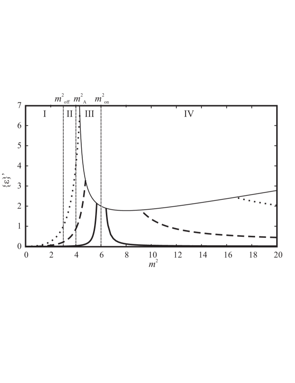
Figure 7: Jump in internal energy $\epsilon$ versus mass flux for various angles $\theta_{1}$: $5^{\circ}$ (solid lines), $25^{\circ}$(dashed lines), and $45^{\circ}$ (dotted lines).

The curve describing the jumps in internal energy at the strongest trans-Alfven and fast shocks is

$$\left\{\,\epsilon\,\right\}^{\,\prime}=\frac{\left(m^{\,2}/\,m_{\rm off}^{\,2}-\,m^{\,2}/\,m_{\rm on}^{\,2}\right)^{2}}{m^{\,2}/\,m_{{}_{\rm A}}^{\,2}-1}\,.$$ (47)

It is indicated by the thin line in Fig. 7.

7 The model of reconnection

Markovskii & Somov (1989) suggested a two-dimensional stationary model of magnetic reconnection, that generalizes and combines the famous reconnection models by Petschek (1964) and Syrovatskii (1971). Later on, Bezrodnykh et al. (2007) constructed a two-dimensional analytical model of reconnection in a plasma with a strong magnetic field that included a thin current layer ($CL$) and four discontinuous MHD flows of finite length $R$ attached to its endpoints. $L$ is a halfwidth of the current layer. Figure 8 displays the configuration of discontinuities inside which the electric currents flow perpendicular to the figure plane. The normal magnetic field component vanishes on the current layer and is equal to a given constant $\beta$ on the MHD shock waves inclined to the $x$-axis at angle $\alpha$. The field at infinity grows linearly with a proportionality coefficient $\gamma$. The quantities $L$, $R$, $\alpha$, $\beta$, and $\gamma$ are free parameters of this model used below.

Magnetic field can be written as $B=(\,B_{x}(x,y),\,B_{y}(x,y),\,0\,)$, i.e., only two of its components, $B_{x}$ and $B_{y}$, are nonzero and depend only on the $x$ and $y$ coordinates. It follows from the magnetic field potentiality that the function $B=B_{x}-iB_{y}$ is an analytic function of variable $z=x+iy$ in the exterior of the sections on the complex plane shown in Fig. 8. Thus, the model considered in this section is reduced to finding the analytic function $B=B_{x}-iB_{y}$ from the linear combination of $B_{x}$ and $B_{y}$ specified at its boundary. Since this problem is symmetric with respect to the $x$ and $y$ axes, it will suffice to consider it only in the first quadrant. Then the boundary condition for the function $B$ is formulated as follows: $B_{y}=0$ on the current layer and surface ($x=0$); $B_{x}\,{\rm sin}\,\alpha+B_{y}\,{\rm cos}\,\alpha=-\beta$ on the discontinuity surface; $B_{x}=0$ on the surface ($y=0,x>L$) and $B=i\gamma z+o(1)$ at $z\to\infty$. Bezrodnykh et al. (2007) constructed the sought-for analytic function in an explicit form by the method of the conformal mapping of the domain outside the system of sections onto the half-plane.

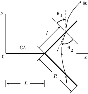
Figure 8: The configuration of electric currents (thick straight segments) consists of a current layer ($CL$) and four segments (discontinuity surfaces) of finite length $R$ attached to its endpoints; $L$ is the current layer half-width (Bezrodnykh et al., 2007).

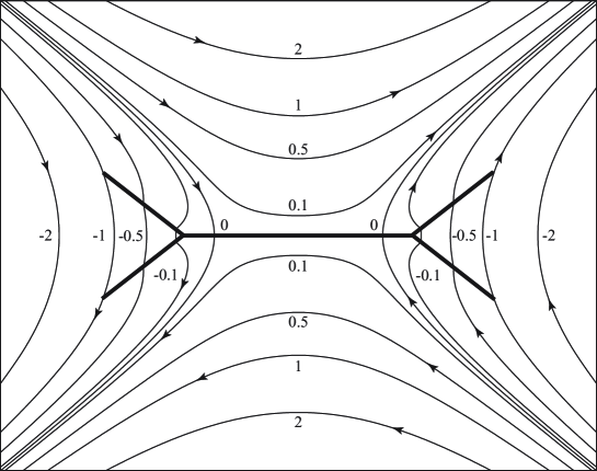
Figure 9: Magnetic field lines (thin curves) with an indication of the values of the vector potential. The regions of direct and reverse currents inside the current layer (the thick horizontal straight segment) are seen. The magnetic field undergoes a jump on the attached discontinuity surfaces (inclined straight segments) (Bezrodnykh et al., 2007).

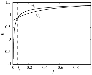
Figure 10: Distribution of the angles $\theta_{1}$ and $\theta_{2}$ at the attached shock. The variable $l$ is the distance measured from the current layer endpoint along the discontinuity surface (Bezrodnykh et al., 2011).

Figure 9 shows magnetic field lines calculated in the special case of reconnection ($L=1$, $R=1$, $\alpha=45^{\circ}$, $\beta=1$, $\gamma=1$) that can be taken as a basis for comparison with many other possible reconnection regimes. The figure demonstrates that the result of solving the problem in the main (central) part of the reconnection region is a current layer ($CL$). It is intersected by two symmetrically located magnetic field lines; the points of intersection (for more details on their properties, see Syrovatskii, 1971; Somov, 2013b) separate the current layer areas with the field circulation relative to them having opposite signs. Thus, the Syrovatskii-type current layer that consists of a direct current and two attached reverse currents is actually located in the central part of the reconnection region.

In specific astrophysical applications, in particular, in solar flares, the model of the so-called super-hot $(T_{e}>10\,\,{\rm keV})$ turbulent-current layer (Somov, 2013b) should be used to determine the physical parameters of this region. The advantage of an analytical model is the possibility to investigate more general patterns that do not depend on the detailed assumptions of a physical reconnection model. Consider some of the properties of discontinuous flows in the vicinity of a current layer predicted by the analytical model of Bezrodnykh et al. (2007).

A magnetic field calculation in the approximation of a strong field near the current structure gives the angles of incidence and refraction of the field on the discontinuity surfaces from which the types of discontinuities are determined. The characteristics of the plasma flowing through the discontinuity change with the distance measured from the point of attachment to the current layer along the discontinuity surface. The set of these characteristics determines the type of discontinuity in each point of the attached surface. Moving from point to point along the surface of the discontinuity we will see the change of the flow conditions, and hence the change of the type of discontinuity. The different types of discontinuous MHD solutions will correspond to the different regions of the attached surface. The transition solutions will realize at the boundaries between these regions.

For example, Fig. 10 taken from Bezrodnykh et al. (2011) shows how the magnetic field inclination angles change with coordinate at the discontinuity for one specific calculation. The discontinuity surface can be arbitrarily divided into three regions in accordance with the types of flows. The trans-Alfven shock is immediately adjacent to the current layer. This is the domain of negative angles $\theta_{1}$ in Fig. 10. As one recedes from the current layer, a fast shock is observed ($\theta_{2}>\theta_{1}$) up to the point of intersection between the plots of $\theta_{1}$ and $\theta_{2}$ at $l=l_{0}$. The discontinuity ends with a slow shock ($\theta_{2}<\theta_{1}$) that gradually passes into a continuous flow ($\theta_{2}=\theta_{1}$) at $l=1$. The absolute values of the angles $\theta_{1}$ and $\theta_{2}$ tend to the same value near the current layer ($l=0$ in Fig. 10). Therefore, the Alfven discontinuity can be realized at this point. We also expect further continuous transitions at $l=0$ in accordance with the scheme of transitions (Fig. 4) but the accuracy of the Fig. 10 does not allow us to say it for sure.

As the plasma flow parameters change continuously, the type of shock must change through transition discontinuities. The first transition occurs between the trans-Alfven and fast shocks in the case we consider. As has been shown above, the switch-on wave (31) must act as a transition discontinuity. Indeed, as can be seen from Fig. 10, the magnetic field at the point of the transition between the trans-Alfven and fast shocks is normal to the discontinuity surface ($\theta_{1}=0$) in the inflow and has a tangential component ($\theta_{2}>0$) in the outflow. This transition cannot be made only by a gradual change in the mass flux through the discontinuity. The angle of incidence of the magnetic field should be simultaneously reduced to reduce the discontinuity between the admissible mass fluxes for the fast and trans-Alfven shocks. In addition, both trans-Alfven and fast shocks satisfy inequality (19). Hence, for the parameters of the medium to change smoothly, the mass flux through the switch-on wave must also satisfy this inequality:

$$m_{\rm off}^{\,2}>m_{\rm A}^{\,2}+m_{\bot}^{\,2}\,,$$

or

$${B_{x}^{\,2}\over 4\pi r_{2}}>{B_{x}^{\,2}+\tilde{B}_{y}^{\,2}\over 4\pi{\tilde{r}}}\,.$$

Simplifying this relation, we obtain a constraint on the possible inclination of the magnetic field behind the discontinuity plane:

$${\rm tg}^{\,2}\,\theta_{2}<\frac{2\,\{\,\rho\,\}}{\rho_{1}}\,.$$ (48)

The second transition between the fast and slow shocks at $l=l_{0}$ cannot be made by a continuous change in the mass flux through the discontinuity. The intersection of the curves in Fig. 10 suggests that there is no jump in magnetic field strength at the point separating the fast and slow shocks. Only the contact discontinuity can correspond to such a field structure. However, as has been shown above, the ratio of the tangents of the angles ${\rm tan}\theta_{2}/{\rm tan}\theta_{1}$ in the fast shock asymptotically tends only to $\rho_{2}/\rho_{1}$ from above and can take on unity typical of a contact discontinuity only at $\{\rho\}=0$. This, along with the boundary conditions (24), gives the absence of a discontinuity at the point of contact between the fast and slow shocks. The jumps in density, velocity, magnetic field, and pressure at this point must be zero.

Thus, the discontinuity surface turns out to be physically separated into two regions: the inner part consists of trans-Alfven and fast shocks, while the outer part is a slow shock. When changing the initial model parameters, we can obtain a reconnection regime in which the discontinuity ends with a fast shock, while the outer part of the discontinuity is absent altogether. This suggests that the inner part of the discontinuity is attributable to the reconnection process itself and is closely related to the presence of a reverse current at the endpoints of the current layer, which was clearly shown by Bezrodnykh et al. (2007), while the outer part depends strongly on the factors affecting the overall topology of current layers: the presence or absence of a “magnetic obstacle”, non-uniformity of the plasma distribution in the reconnection region.

We can trace some analogies of our conclusions with the results of present-day numerical MHD simulations of fast reconnection (Shimizu & Ugai, 2003; Ugai et al., 2005; Ugai, 2008; Zenitani & T. Miyoshi, 2011). As a result of reconnection, the plasma being ejected from a current layer is gathered into the so-called “plasmoid” separated from the surrounding plasma by a system of slow shocks. The structure and intensity of the latter depend on the plasmoid sizes and density. In addition, the characteristics of the outer part of the discontinuity surface in Bezrodnykh et al. (2011) depend on the model geometry. Closer to the current layer, in the region of reverse currents, the numerical models give a complex system of shocks. Since the derived trans-Alfven waves are non-evolutionary, the structure of the inner part of the discontinuity described by Bezrodnykh et al. (2007, 2011) must also become more complicated and can have similarities to the results of numerical simulations. On the whole, the interrelationship between the process of magnetic reconnection and the formation of a system of accompanying discontinuous flows requires a further comprehensive study.

Equation (44) allows us to draw some definite conclusions concerning variations in the internal plasma energy upon the passage though the discontinuity surface. First, the internal energy increases since, according to the Zemplen’s theorem, $-\{r\}>0$, and $\tilde{p}$ and $\{B_{y}\}^{2}$ are positive quantities. Second, the internal energy change is made of two parts, namely, a thermodynamic part, which is defined by the plasma pressure and a magnetic one, which is related to variations in the magnetic field structure in the vicinity of the discontinuity surface.

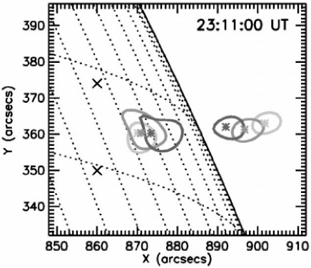
Figure 11: RHESSI images in different energy bands at 23:11:00 UT. The three contours ($80\%$ of the peak flux in each image) on the solar disk indicate the top of loops in the energy bands (contour line shade from light to dark): 6–8, 10–12, and 16–20 keV. The contours ($80\%$ of the peak flux of the coronal source in each image) above the limb are for the (from light to dark) 10–12, 12–14, and 14–16 keV bands. The asterisk marks the centroid of each source. The crosses mark the two footpoints of the X-ray loop (Sui & Holman, 2003).

The maximum heating at discontinuities can be expected in a magnetic field with a sharply varying geometry. These conditions are met in the region of magnetic reconnection. Similar discontinuity structures can be introduced as independent elements into analytical reconnection model. Earlier we showed that the waves that are near the face ends of the current layer (where reverse current are generated) are trans-Alfven shock waves. Moving away from the current layer, the jump of the magnetic field intensity at the discontinuity decreases and the density jump vanishes. Thus, the best conditions for plasma heating occur near the region of reverse currents. However, this conclusion is purely qualitative. Since the input parameters of the model Bezrodnykh et al. (2007, 2011) are some abstract quantities, we can not produce any numerical estimates about the real plasma heating. This process requires further study. Nonetheless, heating by shock waves can help form a super-hot plasma observed with modern X-ray space observatories. (Fig. 11, Sui & Holman, 2003).

8 CONCLUSIONS

The correspondence between the standard classification of discontinuous flows in ideal MHD and the characteristic parameter of plasma flow – the value of the mass flow through the discontinuity – is set up. On this basis, all of allowed transition solutions are found. As a result, the generalized scheme of the continuous transitions between MHD discontinuities is built. It contains the discontinuities that were not represented in the earlier schemes, such as the contact discontinuity, swich-on and swich-off shocks. Some types of discontinuous flows, for example the trans-Alven shock waves, are non-evolutionary. They are also included in the generalized scheme of transitions.

Within a framework of the simplified analytical model of the magnetic reconnection various areas of connected to the current layer discontinuity surface are identified with different types of MHD shock waves. In particular, regions of the trans-Alven shock waves are located near the ends of the current layer (in the presence of reverse currents). Division of the attached to the current layer discontinuity surfaces into two areas is found. That division is result of the different origin of discontinuities. The quasi-stationary inner region is due to the reverse currents in the current layer, and the outer region is caused mainly by the boundary conditions of the magnetic reconnection process and by the speed of reconnection.

We have considered dependence of the plasma heating as the thermodynamic parameters of plasma as the type of MHD discontinuity. The larger the jumps in plasma density and magnetic energy density at the discontinuity, the stronger the heating. Such conditions occur near a region of the reverse currents in the reconnection process. We believe that this result will be useful for quantitative explaining the temperature distributions of the super-hot plasma in solar flares observed by modern space X-ray observatories.

9 ACKNOWLEDGEMENTS

We are grateful to the referees for very helpful remarks. This work was supported by the Russian Foundation for Basic Research (project no. 14-02-31425-mol-a).

References

- Anderson (1963) Anderson J.E., Magnetohydrodynamic shock waves (M.I.T. Press, Massachusetts, 1963).
- Bezrodnykh et al. (2007) Bezrodnykh S.I., Vlasov V.I., & Somov B.V., Analytical model of magnetic reconnection in the presence of shock waves attached to a current layer, Astron. Lett. 33, 130-136 (2007).
- Bezrodnykh et al. (2011) Bezrodnykh S.I., Vlasov V.I., & Somov B.V., Generalized analytical models of Syrovatskii’s current layer, Astron. Lett. 37, 113-130 (2011).
- Brushlinskii et al. (1980) Brushlinskii K.V., Zaborov A.M., & Syrovatskii S.I., Numerical analysis of the current layer near a magnetic null line, Sov. J. Plasma Phys. 6, 165-173 (1980).
- Goedbloed & Poedts (2004) Goedbloed J.P., & Poedts S., Principles of magnetohydrodynamics: with applications to laboratory and astrophysical plasmas (Cambridge Univ. Press, Cambridge, 2004).
- Ledentsov & Somov (2013) Ledentsov L.S., & Somov B.V., Continuous transitions between discontinuous magnetohydrodynamic flows of plasma and Its heating, JETP 117, 1164-1172 (2013).
- Lin et al. (2002) Lin R.P., Dennis B., Hurford G., Smith, D.M., & Zehnder, A., The Reuven Ramaty High-Energy Solar Spectroscopic Imager (RHESSI), Sol. Phys. 210, 3-32 (2002).
- Longmire (1963) Longmire C.L., Elementary plasma physics (Interscience, New York, 1963).
- Markovskii & Somov (1989) Markovskii S.A., & Somov B.V., Some properties of magnetic reconnection in current layer with shock waves, Solar plasma physics (Moscow, Nauka, in Russian), 45-56 (1989).
- Masuda et al. (1994) Masuda S., Kosugi T., Hara H., & et al., A loop-top hard X-ray sources in a compact solar flare as evidence for magnetic reconnection, Nature 371, 495-497 (1994).
- Petrosian et al. (2002) Petrosian V., Donaghy T.Q., & McTiernan J.M., Loop-top hard X-ray emission in solar flares: images and statistics, Astrophys. J. 569, 459-473 (2002).
- Petschek (1964) Petschek H.E., Magnetic field annihilation, AAS-NASA Symp. on the physics of solar flares, Washington, NASA SP-50, 425-439 (1964).
- Polovin (1961) Polovin R.V., Reviews of topical problems: shock waves in magnetohydrodynamics, Sov. Phys. Usp. 3, 677-688 (1961).
- Priest (1982) Priest E.R., Solar magnetohydrodynamics (D. Reidel, Dordrecht, 1982).
- Shimizu & Ugai (2003) Shimizu T., & Ugai M., Magnetohydrodynamic study of adiabatic supersonic and subsonic expansion accelerations in spontaneous fast magnetic reconnection, Phys. Plasmas 10, 921-929 (2003).
- Sirotina & Syrovatskii (1960) Sirotina E.P., & Syrovatskii S.I., Structure of low intensity shock waves in MHD, Sov. Phys. JETP 12, 521-526 (1960).
- Somov (1994) Somov B.V., Fundamentals of cosmic electrodynamics (Kluwer Academic Publ., Dordrecht, 1994).
- Somov (2013a) Somov B.V., Plasma astrophysics, part I: fundamental and practice, Second edition (Springer SBM, New York, 2013).
- Somov (2013b) Somov B.V., Plasma astrophysics, part II: reconnection and flares, Second edition (Springer SBM, New York, 2013).
- Sterck et al. (1998) de Sterck H., Low B.C., & Poedts S., Complex magnetohydrodynamic bow shock topology in field-aligned low- flow around a perfectly conducting cylinder, Phys. Plasmas 5, 4015-4027 (1998).
- Sui & Holman (2003) Sui L., & Holman G.D., Evidence for the formation of a large-scale current layer in a solar flare, Astrophys. J. 596, L251-L254 (2003).
- Syrovatskii (1956) Syrovatskii S.I., Some properties of discontinuity surfaces in magnetohydrodynamics, Tr. Fiz. Inst. im. P. N. Lebedeva, Akad. Nauk SSSR 8, 13-64 (1956) [in Russian].
- Syrovatskii (1957) Syrovatskii S.I., Magnetohydrodynamics, Usp. Fiz. Nauk 62, 247-303 (1957) [in Russian].
- Syrovatskii (1962) Syrovatskii S.I., The stability of plasma in a nonuniform magnetic field and the mechanism of solar flares, Sov. Astron. 6, 768-769 (1962).
- Syrovatskii (1971) Syrovatskii S.I., Formation of current layers in a plasma with a frozen-in strong field, Sov. Phys. JETP 35, 933-940 (1971).
- Tideman & Krall (1971) Tideman D.A., & Krall N.A., Shock waves in collisionless plasma (Wiley-Interscience, New York, London, Sydney, 1971).
- Tsuneta et al. (1992) Tsuneta S., Takahashi T., Acton L.W., Bruner M.E., Harvey K.L., & Ogawara Y., Global restructuring of the coronal magnetic fields observed with the YOHKOH soft X-ray telescope, Publ. Astron. Soc. Japan 44, L211-L214 (1992).
- Tsuneta (1996) Tsuneta S., Structure and dynamics of magnetic reconnection in a solar flare, Astrophys. J. 456, 840-849 (1996).
- Ugai et al. (2005) Ugai M., Kondoh K., & Shimizu T., Spontaneous fast reconnection model in three dimensions, Phys. Plasmas 12, id. 042903 7 pp. (2005).
- Ugai (2008) Ugai M., Impulsive chromospheric heating of two-ribbon flares by the fast reconnection mechanism, Phys. Plasmas 15, id. 032902 9 pp. (2008).
- Zel dovich & Raizer (1967) Zel dovich Ya.B., & Raizer Yu.P., Physics of shock Waves and hightemperature hydrodynamic phenomena (Academic, New York, 1967).
- Zenitani & T. Miyoshi (2011) Zenitani S., & Miyoshi T., Magnetohydrodynamic structure of a plasmoid in fast reconnection in low-beta plasmas, Phys. Plasmas 18, id. 022105 9 pp. (2011).