REBA: A Refinement-Based Architecture for Knowledge Representation and Reasoning in Robotics

Abstract

This paper describes an architecture for robots that combines the complementary strengths of probabilistic graphical models and declarative programming to represent and reason with logic-based and probabilistic descriptions of uncertainty and domain knowledge. An action language is extended to support non-boolean fluents and non-deterministic causal laws. This action language is used to describe tightly-coupled transition diagrams at two levels of granularity, with a fine-resolution transition diagram defined as a refinement of a coarse-resolution transition diagram of the domain. The coarse-resolution system description, and a history that includes (prioritized) defaults, are translated into an Answer Set Prolog (ASP) program. For any given goal, inference in the ASP program provides a plan of abstract actions. To implement each such abstract action, the robot automatically zooms to the part of the fine-resolution transition diagram relevant to this action. A probabilistic representation of the uncertainty in sensing and actuation is then included in this zoomed fine-resolution system description, and used to construct a partially observable Markov decision process (POMDP). The policy obtained by solving the POMDP is invoked repeatedly to implement the abstract action as a sequence of concrete actions, with the corresponding observations being recorded in the coarse-resolution history and used for subsequent reasoning. The architecture is evaluated in simulation and on a mobile robot moving objects in an indoor domain, to show that it supports reasoning with violation of defaults, noisy observations and unreliable actions, in complex domains.

1 Introduction

Robots are increasingly being used to assist humans in homes, offices and other complex domains. To truly assist humans in such domains, robots need to be re-taskable and robust. We consider a robot to be re-taskable if its reasoning system enables it to achieve a wide range of goals in a wide range of environments. We consider a robot to be robust if it is able to cope with unreliable sensing, unreliable actions, changes in the environment, and the existence of atypical environments, by representing and reasoning with different description of knowledge and uncertainty. While there have been many attempts, satisfying these desiderata remains an open research problem.

Robotics and artificial intelligence researchers have developed many approaches for robot reasoning, drawing on ideas from two very different classes of systems for knowledge representation and reasoning, based on logic and probability theory respectively. Systems based on logic incorporate compositionally structured commonsense knowledge about objects and relations, and support powerful generalization of reasoning to new situations. Systems based on probability reason optimally (or near optimally) about the effects of numerically quantifiable uncertainty in sensing and action. There have been many attempts to combine the benefits of these two classes of systems, including work on joint (i.e., logic-based and probabilistic) representations of state and action, and algorithms for planning and decision-making in such formalisms. These approaches provide significant expressive power, but they also impose a significant computational burden. More efficient (and often approximate) reasoning algorithms for such unified probabilistic-logical paradigms are being developed. However, practical robot systems that combine abstract task-level planning with probabilistic reasoning, link, rather than unify, their logic-based and probabilistic representations, primarily because roboticists often need to trade expressivity or correctness guarantees for computational speed. Information close to the sensorimotor level is often represented probabilistically to quantitatively model and reason about the uncertainty in sensing and actuation, with the robot’s beliefs including statements such as “the robotics book is on the shelf with probability $0.9$”. At the same time, logic-based systems are used to reason with (more) abstract commonsense knowledge, which may not necessarily be natural or easy to represent probabilistically. This knowledge may include hierarchically organized information about object sorts (e.g., a cookbook is a book), and default information that holds in all but a few exceptional situations (e.g., “books are typically found in the library”). These representations are linked, in that the probabilistic reasoning system will periodically commit particular claims about the world being true, with some residual uncertainty, to the logical reasoning system, which then reasons about those claims as if they were true. There are thus languages of different expressive strengths, which are linked within an architecture.

The existing work in architectures for robot reasoning has some key limitations. First, many of these systems are driven by the demands of robot systems engineering, and there is little formalization of the corresponding architectures. Second, many systems employ a logical language that is indefeasible, e.g., first order predicate logic, and incorrect commitments can lead to irrecoverable failures. Our proposed architecture addresses these limitations. It represents and reasons about the world, and the robot’s knowledge of it, at two granularities. A fine-resolution description of the domain, close to the data obtained from the robot’s sensors and actuators, is reasoned about probabilistically, while a coarse-resolution description of the domain, including commonsense knowledge, is reasoned about using non-monotonic logic. Our architecture precisely defines the coupling between the representations at the two granularities, enabling the robot to represent and efficiently reason about commonsense knowledge, what the robot does not know, and how actions change the robot’s knowledge. The interplay between the two types of knowledge is viewed as a conversation between, and the (physical and mental) actions of, a logician and a statistician. Consider, for instance, the following exchange:

• the goal is to find the robotics book. I do not know where it is, but I know that books are typically in the library and I am in the library. We should first look for the robotics book in the library.

• look for the robotics book in the library. You only need to reason about the robotics book and the library.

• In my representation of the world, the library is a set of grid cells. I shall determine how to locate the book probabilistically in these cells considering the probabilities of movement failures and visual processing failures.

• I visually searched for the robotics book in the grid cells of the library, but did not find the book. Although there is a small probability that I missed the book, I am prepared to commit that the robotics book is not in the library.

• here are my observations from searching the library; the robotics book is not in the library.

• the robotics book was not found in the library either because it was not there, or because it was moved to another location. The next default location for books is the bookshelf in the lab. We should go look there next.

where the representations used by the logician and the statistician, and the communication of information between them, is coordinated by a controller. This imaginary exchange illustrates key features of our approach:

• Reasoning about the states of the domain, and the effects of actions, happens at different levels of granularity, e.g., the logician reasons about rooms, whereas the statistician reasons about grid cells in those rooms.

• For any given goal, the logician computes a plan of abstract actions, and each abstract action is executed probabilistically as a sequence of concrete actions planned by the statistician.

• The effects of the coarse-resolution (logician’s) actions are non-deterministic, but the statistician’s fine-resolution action effects, and thus the corresponding beliefs, have probabilities associated with them.

• The coarse-resolution knowledge base (of the logician) may include knowledge of things that are irrelevant to the current goal. Probabilistic reasoning at fine resolution (by statistician) only considers things deemed relevant to the current coarse-resolution action.

• Fine-resolution probabilistic reasoning about observations and actions updates probabilistic beliefs, and highly likely statements (e.g., probability $>0.9$) are considered as being completely certain for subsequent coarse-resolution reasoning (by the logician).

1.1 Technical Contributions

The design of our architecture is based on tightly-coupled transition diagrams at two levels of granularity. A coarse-resolution description includes commonsense knowledge, and the fine-resolution transition diagram is defined as a refinement of the coarse-resolution transition diagram. For any given goal, non-monotonic logical reasoning with the coarse-resolution system description and the system’s recorded history, results in a sequence of abstract actions. Each such abstract action is implemented as a sequence of concrete actions by zooming to a part of the fine-resolution transition diagram relevant to this abstract action, and probabilistically modeling the non-determinism in action outcomes. The technical contributions of this architecture are summarized below.

Action language extensions.

An action language is a formalism used to model action effects, and many action languages have been developed and used in robotics, e.g., STRIPS, PDDL [24], BC [39], and $\mathcal{AL}_{d}$ [22]. We extend $\mathcal{AL}_{d}$ in two ways to make it more expressive. First, we allow fluents (domain attributes that can change) that are non-Boolean, which allows us to compactly model a wider range of situations. Second, we allow non-deterministic causal laws, which captures the non-deterministic effects of the robot’s actions, not only in probabilistic but also qualitative terms. This extended version of $\mathcal{AL}_{d}$ is used to describe the coarse-resolution and fine-resolution transition diagrams of the proposed architecture.

Defaults, histories and explanations.

Our architecture makes three contributions related to reasoning with default knowledge and histories. First, we expand the notion of the history of a dynamic domain, which typically includes a record of actions executed and observations obtained (by the robot), to support the representation of (prioritized) default information. We can, for instance, say that a textbook is typically found in the library and, if it is not there, it is typically found in the auxiliary library. Second, we define the notion of a model of a history with defaults in the initial state, enabling the robot to reason with such defaults. Third, we limit reasoning with such expanded histories to the coarse resolution, and enable the robot to efficiently (a) use default knowledge to compute plans to achieve the desired goal; and (b) reason with history to generate explanations for unexpected observations. For instance, in the absence of knowledge about the locations of a specific object, the robot can construct a plan using the object’s default location to speed up search. Also, the robot can build a revised model of the history to explain subsequent observations that contradict expectations based on initial assumptions.

Tightly-coupled transition diagrams.

The next set of contributions are related to the relationship between different models of the domain used by the robot, i.e., the tight coupling between the transition diagrams at two resolutions. First, we provide a formal definition of one transition diagram being a refinement of another, and use this definition to formalize the notion of the coarse-resolution transition diagram being refined to obtain the fine-resolution transition diagram—the fact that both transition diagrams are described in the same language facilitates their construction and this formalization. A coarse-resolution state is, for instance, magnified to provide multiple states at the fine-resolution—the corresponding ability to reason about space at two different resolutions is central for scaling to larger environments. We find two resolutions to be practically sufficient for many robot tasks, and leave extensions to other resolutions as an open problem. Second, we define randomization of a fine-resolution transition diagram, replacing deterministic causal laws by non-deterministic ones. Third, we formally define and automate zooming to a part of the fine-resolution transition diagram relevant to a specific coarse-resolution transition, allowing the robot, while executing any given abstract action, to avoid considering parts of the fine-resolution diagram irrelevant to this action, e.g., a robot moving between two rooms only considers its location in the cells in those rooms.

Dynamic generation of probabilistic representations.

The next set of innovations connect the contributions described so far to quantitative models of action and observation uncertainty. First, we use a semi-supervised algorithm, the randomized fine-resolution transition diagram, prior knowledge (if any), and experimental trials, to collect statistics and compute probabilities of fine-resolution action outcomes and observations. Second, we provide an algorithm that, for any given abstract action, uses these computed probabilities and the zoomed fine-resolution description to automatically construct the data structures for, and thus significantly limit the computational requirements of, probabilistic reasoning. Third, based on the coupling between transition diagrams at the two resolutions, the outcomes of probabilistic reasoning update the coarse-resolution history for subsequent reasoning.

Methodology and architecture.

The final set of contributions are related to the overall architecture. First, for the design of the software components of robots that are re-taskable and robust, we articulate a methodology that is rather general, provides a path for proving correctness of these components, and enables us to predict the robot’s behavior. Second, the proposed knowledge representation and reasoning architecture combines the representation and reasoning methods from action languages, declarative programming, probabilistic state estimation and probabilistic planning, to support reliable and efficient operation. The domain representation for logical reasoning is translated into a program in SPARC [2], an extension of CR-Prolog, and the representation for probabilistic reasoning is translated into a partially observable Markov decision process (POMDP) [33]. CR-Prolog [5] (and thus SPARC) incorporates consistency-restoring rules in Answer Set Prolog (ASP)—in this paper, the terms ASP, CR-Prolog and SPARC are often used interchangeably—and has a close relationship with our action language, allowing us to reason efficiently with hierarchically organized knowledge and default knowledge, and to pose state estimation, planning, and explanation generation within a single framework. Also, using an efficient approximate solver to reason with POMDPs supports a principled and quantifiable trade-off between accuracy and computational efficiency in the presence of uncertainty, and provides a near-optimal solution under certain conditions [33, 49]. Third, our architecture avoids exact, inefficient probabilistic reasoning over the entire fine-resolution representation, while still tightly coupling the reasoning at different resolutions. This intentional separation of non-monotonic logical reasoning and probabilistic reasoning is at the heart of the representational elegance, reliability and inferential efficiency provided by our architecture.

The proposed architecture is evaluated in simulation and on a physical robot finding and moving objects in an indoor domain. We show that the architecture enables a robot to reason with violation of defaults, noisy observations, and unreliable actions, in larger, more complex domains, e.g., with more rooms and objects, than was possible before.

1.2 Structure of the Paper

The remainder of the paper is organized as follows. Section 2 introduces a domain used as an illustrative example throughout the paper, and Section 3 discusses related work in knowledge representation and reasoning for robots. Section 4 presents the methodology associated with the proposed architecture, and Section 5 introduces definitions of basic notions used to build mathematical models of the domain. Section 5.1 describes the action language used to describe the architecture’s coarse-resolution and fine-resolution transition diagrams, and Section 5.2 introduces histories with initial state defaults as an additional type of record, describes models of system histories, and reduces planning with the coarse-resolution domain representation to computing the answer set of the corresponding ASP program. Section 6 provides the logician’s domain representation base on these definitions. Next, Section 7 describes the (a) refinement of the coarse-resolution transition diagram to obtain the fine-resolution transition diagram; (b) randomization of the fine-resolution system description; (c) collection of statistics to compute the probability of action outcomes and observations; and (d) zooming to the part of the randomized system description relevant to the execution of any given abstract action. Next, Section 8 describes how a POMDP is constructed and solved to obtain a policy that implements the abstract action as a sequence of concrete actions. The overall control loop of the architecture is described in Section 9. Section 10 describes the experimental results in simulation and on a mobile robot, followed by conclusions in Section 11. In what follows, we refer to the functions and abstract actions of the coarse-resolution transition diagram using $H$ as the subscript or superscript. The more concrete functions and actions of the fine-resolution transition diagram are referred to using $L$ as the subscript or superscript.

2 Illustrative Example: Office Domain

The following domain (with some variants) will be used as an illustrative example throughout the paper.

Example 1.

[Office domain] Consider a robot that is assigned the goal of moving specific objects to specific places in an office domain. This domain contains:

• The sorts: $place$, $thing$, $robot$, and $object$, with $object$ and $robot$ being subsorts of $thing$. Sorts $textbook$ and $cup$ are subsorts of the sort $object$. Sort names and constants are written in lower-case, while variable names are in uppercase.

• Four specific places: $of\!\!fice$, $main\_library$, $aux\_library$, and $kitchen$. We assume that these places are accessible without the need to navigate any corridors, and that doors between these places are open.

• A number of instances of subsorts of the sort $object$. Also, an instance of the sort $robot$, called $rob_{1}$; we do not consider other robots, but any such robots are assumed to have similar sensing and actuation capabilities.

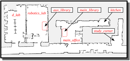
(a) Domain map

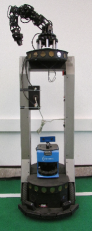
(b) Peoplebot

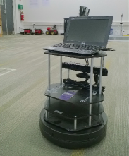
(c) Turtlebot

Figure 1: (a) Subset of the map of an entire floor of a building—specific places are labeled as shown, and used in the goals assigned to the robot; (b)-(c) the “Peoplebot” and “Turtlebot” robot platforms used in the experimental trials.

As an extension of this illustrative example that will be used in the experimental trials on physical robots, consider the robot shown in Figure 1(b) operating in an office building whose map is shown in Figure 1(a). Assume that the robot can (a) build and revise the domain map based on laser range finder data; (b) visually recognize objects of interest; and (c) execute actuation commands, although neither the information extracted from sensor inputs nor the action execution is completely reliable. Next, assume that the robot is in the study corner and is given the goal of fetching the robotics textbook. Since the robot knows that books are typically found in the main library, ASP-based reasoning provides a plan of abstract actions that require the robot to go to the main library, pick up the book and bring it back. For the first abstract action, i.e., for moving to the main library, the robot can focus on just the relevant part of the fine-resolution representation, e.g., the cells through which the robot must pass, but not the robotics book that is irrelevant at this stage of reasoning. It then creates and solves a POMDP for this movement sub-task, and executes a sequence of concrete movement actions until it believes that it has reached the main library with high probability. This information is used to reason at the coarse resolution, prompting the robot to execute the next abstract action to pick up the robotics book. Now, assume that the robot is unable to pick up the robotics book because it fails to find the book in the main library despite a thorough search. This observation violates what the robot expects to see based on default knowledge, but the robot explains this by understanding that the book was not in the main library to begin with, and creates a plan to go to the auxiliary library, the second most likely location for textbooks. In this case, assume that the robot finds the book and completes the task. The proposed architecture enables such robot behavior.

3 Related Work

The objective of this paper is to enable robots to represent and reason with logic-based and probabilistic descriptions of incomplete domain knowledge and degrees of belief. We review some related work below.

There are many recent examples of researchers using probabilistic graphical models such as POMDPs to formulate tasks such as planning, sensing, navigation, and interaction on robots [1, 25, 31, 52]. These formulations, by themselves, are not well-suited for reasoning with commonsense knowledge, e.g., default reasoning and non-monotonic logical reasoning, a key desired capability in robotics. In parallel, research in classical planning and logic programming has provided many algorithms for knowledge representation and reasoning, which have been used on mobile robots. These algorithms typically require a significant amount of prior knowledge of the domain, the agent’s capabilities, and the preconditions and effects of the actions. Many of these algorithms are based on first-order logic, and do not support capabilities such as non-monotonic logical reasoning, default reasoning, and the ability to merge new, unreliable information with the current beliefs in a knowledge base. Other logic-based formalisms address some of these limitations. This includes, for instance, theories of reasoning about action and change, as well as Answer Set Prolog (ASP), a non-monotonic logic programming paradigm, which is well-suited for representing and reasoning with commonsense knowledge [9, 23]. An international research community has developed around ASP, with applications in cognitive robotics [17] and other non-robotics domains. For instance, ASP has been used for planning and diagnostics by one or more simulated robot housekeepers [16], and for representation of domain knowledge learned through natural language processing by robots interacting with humans [12]. ASP-based architectures have also been used for the control of unmanned aerial vehicles in dynamic indoor environments [6]. Recent research has removed the need to solve ASP programs entirely anew when the problem specification changes, allowing new information to expand existing programs, and supporting reuse of ground rules and conflict information to support interactive theory exploration [19]. However, ASP, by itself, does not support quantitative models of uncertainty, whereas a lot of information available to robots is represented probabilistically to quantitatively model the uncertainty in sensor input processing and actuation.

Many approaches for reasoning about actions and change in robotics and artificial intelligence (AI) are based on action languages, which are formal models of parts of natural language used for describing transition diagrams. There are many different action languages such as STRIPS, PDDL [24], BC [39], and $\mathcal{AL}_{d}$ [22], which have been used for different applications [11, 35]. In robotics applications, we often need to represent and reason with recursive state constraints, non-boolean fluents and non-deterministic causal laws. We expanded $\mathcal{AL}_{d}$, which already supports recursive state constraints, to address there requirements. We also expanded the notion of histories to include initial state defaults. Action language BC also supports the desired capabilities but it allows causal laws specifying default values of fluents at arbitrary time steps, and is thus too powerful for our purposes and occasionally poses difficulties with representing all exceptions to such defaults when the domain is expanded.

Refinement of models or action theories has been researched in different fields. In the field of software engineering and programming languages, there are approaches for type and model refinement [18, 44, 45, 47]. These typically do not consider the theories of actions and change that are important for robot domains. More recent work in AI has examined the refinement of action theories of agents in the context of situation calculus [7, 8]. These approaches assume the existence of a bisimulation relation between the action theories for a given refinement mapping between the theories, which often does not hold for robotics domains. They also do not support key capabilities that are needed in robotics such as: (i) reasoning with commonsense knowledge; (ii) automatic construction and use of probabilistic models of sensing and actuation; and (iii) automatic zooming to the relevant part of the refined description. Although we do not describe it here, it is possible to introduce simplifying assumptions and a mapping that reduces our approach to one that is similar to the existing approach.

Robotics and AI researchers have designed algorithms and architectures based on the understanding that robots interacting with the environment through sensors and actuators need both logical and probabilistic reasoning capabilities. For instance, architectures have been developed to support hierarchical representation of knowledge and axioms in first-order logic, and probabilistic processing of perceptual information [37, 38, 64], while deterministic and probabilistic algorithms have been combined for task and motion planning on robots [34]. Another example is the behavior control of a robot that included semantic maps and commonsense knowledge in a probabilistic relational representation, and then used a continual planner to switch between decision-theoretic and classical planning procedures based on degrees of belief [30]. The performance of such architectures can be sensitive to the choice of threshold for switching between the different planning procedures, and the use of first order logic in these architectures limits the expressiveness and use of commonsense knowledge. More recent work has used a three-layered organization of knowledge (instance, default and diagnostic), with knowledge at the higher level modifying that at the lower levels, and a three-layered architecture (competence layer, belief layer and deliberative layer) for distributed control of information flow, combining first-order logic and probabilistic reasoning for open world planning [29]. Declarative programming has also been combined with continuous-time planners for path planning in mobile robot teams [54]. Most of these architectures do not provide a tight coupling between the deterministic and probabilistic components, which has a negative effect on the computational efficiency, reliability and the ability to trust the decisions made. More recent work has combined a probabilistic extension of ASP with POMDPs for commonsense inference and probabilistic planning in human-robot dialog [72], used a probabilistic extension of ASP to determine some model parameters of POMDPs [68], and used an ASP-based architecture to support learning of action costs on a robot [35]. ASP-based reasoning has also been combined with reinforcement learning (RL), e.g., to enable an RL agent to only explore relevant actions [41], or to compute a sequence of symbolic actions that guides a hierarchical MDP controller computing actions for interacting with the environment [67]; an architecture combining ASP-based reasoning with relational RL has been used to interactively and cumulatively discover domain axioms and affordances [59, 60].

Combining logical and probabilistic reasoning is a fundamental problem in AI, and many principled algorithms have been developed to address this problem. For instance, a Markov logic network combines probabilistic graphical models and first order logic, assigning weights to logic formulas [51]. Bayesian Logic relaxes the unique name constraint of first-order probabilistic languages to provide a compact representation of distributions over varying sets of objects [48]. Other examples include independent choice logic [50], PRISM [26], probabilistic first-order logic [28], first-order relational POMDPs [32, 53], and a system (Plog) that assigns probabilities to different possible worlds represented as answer sets of ASP programs [10, 40]. Despite significant prior research, knowledge representation and reasoning for robots collaborating with humans continues to present open problems. Algorithms based on first-order logic do not support non-monotonic logical reasoning, and do not provide the desired expressiveness for capabilities such as default reasoning—it is not always possible to express degrees of belief and uncertainty quantitatively, e.g., by attaching probabilities to logic statements. Other algorithms based on logic programming do not support one or more of the capabilities such as reasoning about relations as in causal Bayesian networks; incremental addition of probabilistic information; reasoning with large probabilistic components; or dynamic addition of variables to represent open worlds. Our prior work has developed architectures that support different subsets of these capabilities. For instance, we developed an architecture that coupled planning based on a hierarchy of POMDPs [62, 70] with ASP-based inference. The domain knowledge included in the ASP knowledge base of this architecture was incomplete and considered default knowledge, but did not include a model of action effects. In other work, ASP-based inference provided priors for POMDP state estimation, and observations and historical data from comparable domains were considered for reasoning about the presence of target objects in the domain [71]. This paper builds on our more recent work on a general, refinement-based architecture for knowledge representation and reasoning in robotics [58, 69]. The architecture enables robots to represent and reason with tightly-coupled transition diagrams at two different levels of granularity. In this paper, we formalize and establish the properties of this coupling, present a general methodology for the design of software components of robots, provide a path for establishing correctness of these components, and describe detailed experimental results in simulation and on physical robot platforms.

4 Design Methodology

Our proposed architecture is based on a design methodology. A designer following this methodology will:

1. Provide a coarse-resolution description of the robot’s domain in action language $\mathcal{AL}_{d}$ together with the description of the initial state.

2. Provide the necessary domain-specific information for, and construct and examine correctness of, the fine-resolution refinement of the coarse-resolution description.

3. Provide domain-specific information and randomize the fine-resolution description of the domain to capture the non-determinism in action execution.

4. Run experiments and collect statistics to compute probabilities of the outcomes of actions and the reliability of observations.

5. Provide these components, together with any desired goal, to a reasoning system that directs the robot towards achieving this goal.

The reasoning system implements an action loop that can be viewed as an interplay between a logician and statistician (Section 1 and Section 9). In this paper, the reasoning system uses ASP-based non-monotonic logical reasoning, POMDP-based probabilistic reasoning, models and descriptions constructed during the design phase, and records of action execution and observations obtained from the robot. The following sections describe components of the architecture, design methodology steps, and the reasoning system. We first define some basic notions, specifically action description and domain history, which are needed to build mathematical models of the domain.

5 Action Language and Histories

This section first describes extensions to action language $\mathcal{AL}_{d}$ to support non-boolean fluents and non-deterministic causal laws (Section 5.1). Next, Section 5.2 expands the notion of the history of a dynamic domain to include initial state defaults, defines models of such histories, and describes how these models can be computed. Section 5.3 describes how these models can be used for reasoning. The subsequent sections describe the use of these models (of action description and history) to provide the coarse-resolution description of the domain, and to build more refined fine-resolution models of the domain.

5.1 $\mathcal{AL}_{d}$ with non-boolean functions and non-determinism

Action languages are formal models of parts of natural language used for describing transition diagrams. In this paper, we extend action language $\mathcal{AL}_{d}$ [21, 22, 23] (we preserve the old name for simplicity) to allow functions (fluents and statics)with non-boolean values, and non-deterministic causal laws.

5.1.1 Syntax and informal semantics of $\mathcal{AL}_{d}$

The description of the syntax of $\mathcal{AL}_{d}$ will require some preliminary definitions.

Sorted Signature: By sorted signature we mean a tuple:

$$\Sigma=\langle\mathcal{C},\mathcal{S},\mathcal{F}\rangle$$

where $\mathcal{C}$ and $\mathcal{F}$ are sets of strings, over some fixed alphabet, which are used to name “user-defined” sorts and functions respectively. $\mathcal{S}$ is a sort hierarchy, a directed acyclic graph whose nodes are labeled by sort names from $\mathcal{C}$. A link $\langle c_{1},c_{2}\rangle$ of $\mathcal{S}$ indicates that $c_{1}$ is a subsort of $c_{2}$. A pair $\langle\mathcal{C},\mathcal{S}\rangle$ will occasionally be referred to as an ontology. Each function symbol $f\in\mathcal{F}$ is assigned a non-negative integer $n$ (called $f$’s arity), sorts $c_{0},\dots,c_{n}$ for its parameters, and sort $c$ for its values. We refer to $c_{0}\times c_{2}\dots\times c_{n}$ as the domain of $f$, written as $dom(f)$, and to $c$ as the range of $f$, written as $range(f)$. If $n>0$ we use the standard mathematical notation $f:c_{0}\times\dots\times c_{n}\rightarrow c$ for this assignment. We refer to a vector $c_{0},\dots,c_{n},c$ as the signature of $f$. For function of arity $0$ (called object constants), the notation turns into $f:c$. We say that $o:c$ is compatible with sort $c^{\prime}$ if $\mathcal{S}$ contains a path from $c$ to $c^{\prime}$. A sort denoted by a sort name $c$ is the collection $\{o_{1},\dots,o_{n}\}$ of all object constants compatible with $c$; this will be written as $c=\{o_{1},\dots,o_{n}\}$.

In addition to all these “user-defined” sorts and functions, sorted signatures often contain standard arithmetic symbols such as $0,1,2,\dots$ of sort $N$ of natural numbers, and relations and functions such as $\geq$ and $+$, which are interpreted in the usual way.

Terms of a sorted signature $\Sigma$ are constructed from variables and function symbols as follows:

• A variable is a term.

• An object constant $o:c$ is a term of sort $c$.

• If $f:c_{0}\times\dots\times c_{n}\rightarrow c$ where $n>0$ is a function symbol and $o_{i}$ is a variable or a constant compatible with sort $c_{i}$ for $0\leq i\leq n$, then $f(o_{0},\dots,o_{n})$ is a term of sort $c$.

Atoms of $\Sigma$ are of the form:

$$f(\bar{x})=y$$

where $y$ and elements of $\bar{x}$ are variables or properly typed object constants, or standard arithmetic atoms formed by $\geq$, $>$, etc. If $f$ is boolean, we use the standard notation $f(\bar{x})$ and $\neg f(\bar{x})$. Literals are expressions of the form $f(\bar{x})=y$ and $f(\bar{x})\not=y$. Terms and literals not containing variables are called ground.

Action Signature: Signatures used by action languages are often referred to as action signatures. They are sorted signatures with some special features that include various classifications of functions from $\mathcal{F}$ and the requirements for inclusion of a number of special sorts and functions. In what follows, we describe the special features of the action signatures that we use in this paper.

To distinguish between actions and attributes of the domain $\mathcal{F}$ is divided into two disjoint parts: $\mathcal{A}$ and $\mathcal{DA}$. Functions from $\mathcal{A}$ are always boolean. Terms formed by function symbols from $\mathcal{A}$ and $\mathcal{DA}$ will be referred to as actions and domain attributes respectively. $\mathcal{DA}$ is further partitioned into $\mathcal{DA}_{s}$ and $\mathcal{DA}_{f}$. Terms formed by functions from $\mathcal{DA}_{s}$ are referred to as statics, and denote domain attributes whose truth values cannot be changed by actions (e.g., locations of walls and doors). Terms formed by functions from $\mathcal{DA}_{f}$ are referred to as fluents. $\mathcal{DA}_{f}$ is further divided into $\mathcal{DA}_{bf}$ and $\mathcal{DA}_{df}$. Terms formed by symbols from $\mathcal{DA}_{bf}$ are called basic fluents and those formed by symbols from $\mathcal{DA}_{df}$ are called defined fluents. The defined fluents are always boolean—they do not obey laws of inertia, and are defined in terms of other fluents. Basic fluents, on the other hand, obey laws of inertia (thus often called inertial fluents in the knowledge representation literature) and are directly changed by actions. Distinction between basic fluents and defined fluents, as introduced in [22], was the key difference between the previous version of $\mathcal{AL}_{d}$ and its predecessor $\mathcal{AL}$.

The new version of $\mathcal{AL}_{d}$ described in this paper introduces an additional partition of basic fluents into basic physical fluents ($\mathcal{DA}_{pbf}$) describing physical attributes of the domain, and basic knowledge fluent ($\mathcal{DA}_{kbf}$) describing the agent’s knowledge. There is a similar partition of $\mathcal{A}$ into physical actions ($\mathcal{A}_{p}$) that can change the physical state of the world (i.e., the value of physical fluents), and knowledge producing actions that are only capable of changing the agent’s knowledge (i.e., the value of knowledge fluents). Since robots observe their world through sensors, we also introduce observable fluents ($\mathcal{DA}_{obsf}$) to represent the fluents whose values can be checked by the robot by processing sensor inputs, or inferred based on the values of other fluents. The set $\mathcal{DA}_{obsf}$ can be divided into two parts: the set $\mathcal{DA}_{dobsf}$ of directly observable fluents, i.e. fluents whose values can be observed directly through sensors, and the set $\mathcal{DA}_{indobsf}$ of indirectly observable fluents i.e., fluents whose values are not observed directly but are (instead) inferred from the values of other directly or indirectly observed fluents. For instance, in Example 1, the robot in any given grid cell can directly observe if a cup is in that grid cell. The observation of the cup in a particular cell can be used to infer the room location of the cup. Our classification of functions is also expanded to literals of the language. If $f$ is static then $f(\bar{x})=y$ is a static literal, if $f$ is a basic fluent then $f(\bar{x})=y$ is a basic fluent literal.

In addition to the classifications of functions, action signatures considered in this paper also include a collection of special sorts like $robot$, $place$, etc., and fluents intrinsic to reasoning about observations. We will refer to the latter as observation related fluents. A typical example is a collection of defined fluents:

$$observable_{f}:robot\times dom(f)\times range(f)\to boolean$$ (1)

where $f$ is an observable function. These fluents are used to specify domain-specific conditions under which a particular robot can observe particular values of particular observable fluents. For instance, in the domain in Example 1, we may need to say that robot $rob_{1}$ can only observe the place location of an object if it is also in the same place:

$$observable_{loc}(rob_{1},O,Pl)~{}~{}\mathbf{if}~{}~{}loc(rob_{1})=Pl$$

For readability, we will slightly abuse the notation and write the above statements as:

$$observable:robot\times obs\_fluent\times value\to boolean$$

where $obs\_fluent$ stands for “observable fluent”, and:

$$observable(rob_{1},loc(O),Pl)~{}~{}\mathbf{if}~{}~{}loc(rob_{1})=Pl$$

In Section 7.1.2, we describe the use of these (and other such) observation-related fluents for describing a theory of observations. Then, in Section 10.1, we describe the processing of inputs from sensors to observe the values of fluents.

Statements of $\mathcal{AL}_{d}$: Action language $\mathcal{AL}_{d}$ allows five types of statements: deterministic causal laws, non-deterministic causal laws, state constraints, definitions, and executability conditions. With the exception of non-deterministic causal law (Statement 3), these statements are built from ground literals.

• Deterministic causal laws are of the form:

  $$a\ \mathbf{causes}\ f(\bar{x})=y~{}~{}\mathbf{if}\ ~{}body$$ (2)

  where $a$ is an action literal, $f$ is a basic fluent literal, and $body$ is a collection of fluent and static literals. If $a$ is formed by a knowledge producing action, $f$ must be a knowledge fluent. Intuitively, Statement 2 says that if $a$ is executed in a state satisfying $body$, the value of $f$ in any resulting state would be $y$. Non-deterministic causal laws are of the form:

  $$a\ \mathbf{causes}\ f(\bar{x})\ =\ \{Y:p(Y)\}~{}\mathbf{if}\ ~{}body$$ (3)

  where $p$ is a unary boolean function symbol from $\mathcal{DA}$, or:

  $$a\ \mathbf{causes}\ f(\bar{x})\ :\ sort\_name~{}\mathbf{if}\ ~{}body$$ (4)

  Statement 3 says that if $a$ is executed in a state satisfying $body$, $f$ may take on any value from the set $\{Y:p(Y)\}\cap range(f)$ in the resulting state. Statement 4 says that $f$ may take any value from $\{sort\_name\cap range(f)\}$. If the $body$ of a causal law is empty, the $\mathbf{if}$ part of the statement is omitted. Note that these axioms are formed from terms and literals that are ground, and (possibly) from the expression $\{Y:p(Y)\}$ that is sometimes referred to as a set term. Occurrences of $Y$ in a set term are called bound. A statement of $\mathcal{AL}_{d}$ is ground if every variable occurring in it is bound. Even though the syntax of $\mathcal{AL}_{d}$ only allows ground sentences, we often remove this limitation in practice. For instance, in the context of Example 1, we may have the deterministic causal law:

  $$move(R,Pl)~{}~{}\mathbf{causes}~{}~{}loc(R)=Pl$$

  which says that for every robot $R$ moving to place $Pl$ will end up in $Pl$. In action languages, each such statement is usually understood as shorthand for a collection of its ground instances, i.e., statements obtained by replacing its variables by object constants of the corresponding sorts. We use a modified version of this approach in which only non-bound variables are eliminated in this way.

• State constraints are of the form:

  $$f(\bar{x})=y\ ~{}\mathbf{if}\ ~{}body$$ (5)

  where $f$ is a basic fluent or static. The state constraint says that $f(\bar{x})=y$ must be true in every state satisfying $body$. For instance, the constraint:

  $$loc(Ob)=Pl~{}~{}\mathbf{if}~{}~{}loc(R)=Pl,~{}~{}in\_hand(R,Ob)$$

  guarantees that the object grasped by a robot shares the robot’s location.

• The definition of the value of a defined fluent $f$ on $\bar{x}$ is a collection of statements of the form:

  $$f(\bar{x})\ ~{}\mathbf{if}\ ~{}body$$ (6)

  where $f(\bar{x})$ is true if it follows from the truth of at least one of its defining rules. Otherwise, $f(\bar{x})$ is false.

• Executability conditions are statements of the form:

  $$\mathbf{impossible}\ a_{0},\ldots,a_{k}\ \mathbf{if}\ ~{}body$$ (7)

  which implies that in a state satisfying $body$, actions $a_{0},\ldots a_{k}$ cannot occur simultaneously. For instance, the following executability condition:

  $$\mathbf{impossible}~{}~{}move(R,Pl)~{}~{}\mathbf{if}~{}~{}loc(R)=Pl$$

  implies that a robot cannot move to a location if it is already there; and

  $$\mathbf{impossible}~{}~{}grasp(R_{1},Th),grasp(R_{2},Th)~{}~{}\mathbf{if}~{}~{}R_{1}\not=R_{2}$$

  prohibits two robots from simultaneously grasping the same thing.

We can now define the notion of a system description.

Definition 1.

[System Description]
A system description of $\mathcal{AL}_{d}$ is a collection of $\mathcal{AL}_{d}$ statements over some action signature $\Sigma$.

Next, we discuss the formal semantics of $\mathcal{AL}_{d}$.

5.1.2 Formal semantics of $\mathcal{AL}_{d}$

The semantics of system description $\mathcal{D}$ of the new $\mathcal{AL}_{d}$ is similar to that of the old one. In fact, the old language can be viewed as the subset of $\mathcal{AL}_{d}$ in which all functions are boolean, causal laws are deterministic, and no distinction is made between physical and knowledge related actions and fluents. The semantics of $\mathcal{D}$ is given by a transition diagram ${\tau(\mathcal{D})}$ whose nodes correspond to possible states of the system. The diagram contains an arc $\langle\sigma_{1},a,\sigma_{2}\rangle$ if, after the execution of action $a$ in state $\sigma_{1}$, the system may move into state $\sigma_{2}$. We define the states and transitions of ${\tau(\mathcal{D})}$ in terms of answer sets of logic programs, as described below—see [21, 23] for more details.

In what follows, unless otherwise stated, by “atom” and “term” we refer to “ground atom” and “ground term” respectively. Recall that an interpretation of the signature of $\mathcal{D}$ is an assignment of a value to each term $f(\bar{x})$ in the signature. An interpretation can be represented by the collection of atoms of the form $f(\bar{x})=y$, where $y$ is the value of $f(\bar{x})$. For any interpretation $\sigma$, let $\sigma^{nd}$ be the collection of atoms of $\sigma$ formed by basic fluents and statics—${nd}$ stands for non-defined. Let $\Pi_{c}(\mathcal{D})$, where $c$ stands for constraints, denote the logic program defined as:

1. For every state constraint (Statement 5) and definition (Statement 6), program $\Pi_{c}(\mathcal{D})$ contains:

   $$f(\bar{x})=y~{}~{}\leftarrow body$$ (8)

2. For every defined fluent $f$, $\Pi_{c}(\mathcal{D})$ contains the closed world assumption (CWA):

   $$\neg f(\bar{x})\leftarrow\mbox{ not }f(\bar{x})$$ (9)

   where, unlike classical negation “$\lnot~{}a$” that implies “a is believed to be false”, default negation “$not~{}a$” only implies that “a is not believed to be true”, i.e., $a$ can be true, false or just unknown.

We can now define states of ${\tau(\mathcal{D})}$.

Definition 2.

[State of $\tau(\mathcal{D})$]
An interpretation $\sigma$ is a state of the transition diagram ${\tau(\mathcal{D})}$ if it is the unique answer set of program $\Pi_{c}(\mathcal{D})\cup\sigma^{nd}$.

As an example, consider a system description $\mathcal{D}_{s}$ from [23] with two defined fluents $f$ and $g$ defined by mutually recursive laws:

$$g~{}~{}\mathbf{if}~{}~{}\lnot f$$

$$f~{}~{}\mathbf{if}~{}~{}\lnot g$$

For this system description, the program $\Pi_{c}(\mathcal{D}_{s})$ consists of the following statements:

$$g~{}~{}\leftarrow~{}~{}\lnot f$$

$$f~{}~{}\leftarrow~{}~{}\lnot g$$

$$\lnot g~{}~{}\leftarrow~{}~{}not~{}g$$

$$\lnot f~{}~{}\leftarrow~{}~{}not~{}f$$

and $\sigma^{nd}=\emptyset$ because all the fluents of $\mathcal{D}_{s}$ are defined. $\Pi_{c}(\mathcal{D}_{s})\cup\sigma^{nd}$ has two answer sets $\{f,\lnot g\}$ and $\{g,\lnot f\}$; based on Definition 2, the transition diagram $\tau(\mathcal{D}_{s})$ has no states. This outcome is expected because the mutually recursive laws are not strong enough to uniquely define $f$ and $g$.

Next, we define a sufficient condition for guaranteeing that the defined fluents of a system description are uniquely defined by the system’s statics and basic fluents. To do so, we introduce some terminology from [23]. A system description $\mathcal{D}$ is said to be well-founded if for any complete and consistent set of fluent literals and statics $\sigma$ satisfying the state constraints of $\mathcal{D}$, program $\Pi_{c}(\mathcal{D})\cup\sigma^{nd}$ has an unique answer set. Next, the fluent dependency graph of $\mathcal{D}$ is the directed graph such that:

• its vertices are arbitrary domain literals.

• it has an edge:

  • from $l$ to $l^{\prime}$ if $l$ is formed by a static or a basic fluent, and $\mathcal{D}$ contains a state constraint with the head $l$ and the body containing $l^{\prime}$;

  • from $f$ to $l^{\prime}$ if $f$ is a defined fluent, and $\mathcal{D}$ contains a state constraint with the head $f$ and body containing $l^{\prime}$ and not $f$; and

  • from $\lnot f$ to $f$ for every defined fluent $f$.

Also, a fluent dependency graph is said to be weakly acyclic if it does not contain paths from defined fluents to their negations. A system description with a weakly acyclic fluent dependency graph is also said to be weakly acyclic. Although well-foundedness is not easy to check, it is easy to check weak acyclicity, and Proposition $8.4.1$ in [23] establishes weak acyclicity as a sufficient condition for well-foundedness [22]. It is easy to show that all system descriptions discussed in this paper are well-founded, a fact that we will use later in this paper.

Next, to define the transition relation of ${\tau(\mathcal{D})}$, we first describe the logic programming encoding $\Pi(\mathcal{D})$ of $\mathcal{D}$. $\Pi(\mathcal{D})$ consists of the encoding of the signature of $\mathcal{D}$ and rules obtained from statements of $\mathcal{D}$, as described below.

Definition 3.

[Logic programming encoding of $\mathcal{D}$]

• Encoding of the signature: we start with the encoding $sig(\mathcal{D})$ of signature of $\mathcal{D}$.

  • For each sort $c$, $sig(\mathcal{D})$ contains: $sort\_name(c)$.

  • For each subsort link $\langle c_{1},c_{2}\rangle$ of the hierarchy of sorts, $sig(\mathcal{D})$ contains: $s\_link(c_{1},c_{2})$.

  • For each constant $x:c$ from the signature of $\mathcal{D}$, $sig(\mathcal{D})$ contains: $m\_link(x,c)$.

  • For every function symbol $f:c_{1}\times\dots c_{n}\rightarrow c$, the signature $sig(\mathcal{D})$ contains the domain: $dom(f,c_{1},\dots,c_{n})$, and range: $range(f,c)$.

  • For every static $g(\bar{x})$ of $\mathcal{D}$, $sig(\mathcal{D})$ contains: $static(g(\bar{x}))$.

  • For every basic fluent $f(\bar{x})$, $sig({\mathcal{D}})$ contains: $fluent(basic,f(\bar{x}))$.

  • For every defined fluent $f(\bar{x})$, $sig(\mathcal{D})$ contains: $fluent(defined,f(\bar{x}))$.

  • For every observable fluent $f(\bar{x})$, $sig(\mathcal{D})$ contains: $obs\_fluent(f(\bar{x}))$.

  • For every directly observable fluent $f(\bar{x})$, $sig(\mathcal{D})$ contains: $dir\_obs\_fluent(f(\bar{x}))$.

  • For every indirectly observable fluent $f(\bar{x})$, $sig(\mathcal{D})$ contains: $indir\_obs\_fluent(f(\bar{x}))$.

  • For every action $a$ of $\mathcal{D}$, $sig(\mathcal{D})$ contains: $action(a)$.

  We also need axioms describing the hierarchy of basic sorts:

  $$subsort(C_{1},C_{2}) \leftarrow s\_link(C_{1},C_{2})$$ (10)

  $$subsort(C_{1},C_{2}) \leftarrow s\_link(C_{1},C),~{}subsort(C,C_{2})$$

  $$member(X,C) \leftarrow m\_link(X,C)$$

  $$member(X,C_{1}) \leftarrow m\_link(X,C_{0}),~{}subsort(C_{0},C_{1})$$

• Encoding of statements of $\mathcal{D}$: To define transitions of our diagram we need two time-steps that stand for the beginning and the end of a transition. We would like, however, to later use the rules of our program to describe longer chains of events. To make this possible we introduce a symbolic constant $n$ and allow time-steps of the program to range over $[0,max\_step]$. This is expressed by statement:

  $$step(0..max\_step)$$

  For defining transitions we set $max\_step$ to $1$:

  $$\#const\ max\_step=1$$

  We also need a relation $val(f(x_{1},\dots,x_{n}),y,i)$, which states that the value of $f(x_{1},\dots,x_{n})$ at step $i$ is $y$; and relation $occurs(a,i)$, which states that action $a$ occurred at step $i$. We then encode statements of $\mathcal{D}$ as follows:

  • For every causal law (Statements 3-4), where the range of $f$ is $\{y_{1},\ldots,y_{k}\}$, $\Pi(\mathcal{D})$ contains a rule:

    $$val(f(\bar{x}),y_{1},I+1)\ \mathbf{or}\ \ldots\mathbf{or}\ val(f(\bar{x}),y_{k},I+1)\leftarrow val(body,I),~{}occurs(a,I),~{}I<n$$ (11)

    where $val(body,I)$ is obtained by replacing every literal $f_{m}(\bar{x}_{m})=z$ from $body$ by $val(f_{m}(\bar{x}_{m}),z,I)$. To encode that due to this action, $f(\bar{x})$ only takes a value that satisfies property $p$, $\Pi(\mathcal{D})$ contains a constraint:

    $$\leftarrow val(f(\bar{x}),Y,I+1),\textrm{ not }val(p(Y),true,I)$$ (12)

    and rules:

    $$satisfied(p,I) \leftarrow val(p(Y),true,I)$$ (13)

    $$\neg occurs(a,I) \leftarrow\textrm{ not }satisfied(p,I)$$

  • For every state constraint and definition (Statements 5, 6), $\Pi(\mathcal{D})$ contains:

    $$val(f(\bar{x}),y,I)\leftarrow val(body,I)$$ (14)

  • $\Pi(\mathcal{D})$ contains the CWA for defined fluents:

    $$val(F,false,I)\leftarrow fluent(defined,F),~{}\textrm{ not}\ val(F,true,I)$$ (15)

  • For every executability condition (Statement 7), $\Pi(\mathcal{D})$ contains:

    $$\neg occurs(a_{0},I)\ \mathbf{or}\ \dots\ \mathbf{or}\ \ \neg occurs(a_{k},I)\leftarrow val(body,I),~{}I<n$$ (16)

  • For every static $g(\bar{x})$, $\Pi(\mathcal{D})$ contains:

    $$g(\bar{x})=y$$ (17)

  • $\Pi(\mathcal{D})$ contains the Inertia Axiom:

    $$val(F,Y,I+1)\leftarrow fluent(basic,F),$$ (18)

    $$val(F,Y,I),~{}not\ \neg val(F,Y,I+1),~{}I<n$$

  • $\Pi(\mathcal{D})$ contains CWA for actions:

    $$\neg occurs(A,I)\leftarrow \;{not}\;occurs(A,I),~{}I<n$$ (19)

  • Finally, we need the rule:

    $$\neg val(F,Y_{1},I)\leftarrow val(F,Y_{2},I),~{}Y_{1}\not=Y_{2}$$ (20)

    which says that a fluent can only have one value at each time step.

This completes the construction of encoding $\Pi(\mathcal{D})$ of system description $\mathcal{D}$. Later we will consider a version of $\mathcal{D}$ in which time step $max\_step$ is set to some positive number k. We denote such a program by $\Pi^{k}(\mathcal{D})$.

Recall that the axioms described above are shorthand for the set of ground instances obtained by replacing variables by ground terms from the corresponding sorts. We now define a transition of $\tau(\mathcal{D})$.

Definition 4.

[Transition of $\tau(\mathcal{D})$]
Let $a$ be a non-empty collection of actions, and $\sigma_{0}$ and $\sigma_{1}$ be states of the transition diagram ${\tau(\mathcal{D})}$ defined by a system description $\mathcal{D}$. To describe a transition $\langle\sigma_{0},a,\sigma_{1}\rangle$, we construct a program $\Pi(\mathcal{D},\sigma_{0},a)$ consisting of:

• Logic programming encoding $\Pi(\mathcal{D})$ of system description $\mathcal{D}$, as described above.

• The encoding $val(\sigma_{0},0)$ of initial state $\sigma_{0}$:

  $$val(\sigma_{0},0)=_{def} \{val(f(\bar{x}),y,0):(f(\bar{x})=y)\in\sigma_{0}\},\,\,\textrm{where }f\textrm{ is a fluent}\,\,\cup$$

  $$\{f(\bar{x})=y:(f(\bar{x})=y)\in\sigma_{0}\}\,\,\textrm{where }f\textrm{ is a static}$$

• Encoding $occurs(a,0)$ of set of actions $a$:

  $$occurs(a,0) =_{def}\{occurs(a_{i},0):a_{i}\in a\}$$

In other words, the program $\Pi(\mathcal{D},\sigma_{0},a)$ includes our description of the system’s laws, the initial state, and the actions that occur in it:

$$\Pi(\mathcal{D},\sigma_{0},a)=_{def}\Pi(\mathcal{D})\cup val(\sigma_{0},0)\cup occurs(a,0)$$

A state-action-state triple $\langle\sigma_{0},a,\sigma_{1}\rangle$ is a transition of ${\tau(\mathcal{D})}$ iff $\Pi(\mathcal{D},\sigma_{0},a)$ has an answer set $AS$ such that $\sigma_{1}=\{f(\bar{x})=y:val(f(\bar{x}),y,1)\in AS\}$. The answer sets of $\Pi(\mathcal{D},\sigma_{0},a)$ thus determine the states the system can move into after executing of $a$ in $\sigma_{0}$.

5.2 Histories with defaults

In action languages, domain knowledge is typically represented by a system description containing general knowledge about the domain and the agent’s abilities, and the domain’s recorded history containing information pertinent to the agent’s activities in the domain. This history $\mathcal{H}$ typically contains the agent’s observations of the value of domain attributes, and the occurrences of actions, as recorded by statements of the form:

$$obs(rob_{1},f(\bar{x}),y,true,i)$$ (21)

$$obs(rob_{1},f(\bar{x}),y,false,i)$$ (22)

and

$$hpd(a,i)$$ (23)

where $f$ is an observable fluent, $y$ is a possible value of this fluent, $a$ is an action, and $i$ is a time-step. Statement 21 says that a particular fluent was observed to have (or not have) a particular value at time-step $i$ by robot $rob_{1}$, and Statement 23 says that action $a$ happened at time-step $i$. For instance, $obs(rob_{1},loc(tb_{1}),of\!\!fice,true,0)$ denotes the observation of textbook $tb_{1}$ in the $of\!\!fice$ by robot $rob_{1}$, and $hpd(move(rob_{1},kitchen),1)$ is the record of successful execution of $rob_{1}$’s move to the kitchen at time step $1$. Note that the standard representation of $obs$ does not include the $robot$ as the first argument—we include it to emphasize that observations are obtained by specific robots. Also, for convenience, we write $obs(rob_{1},f(\bar{x}),y,true,i)$ as $obs(rob_{1},f(\bar{x})=y,i)$, and write $obs(rob_{1},f(\bar{x}),y,false,i)$ as $obs(rob_{1},f(\bar{x})\not=y,i)$. In addition, the notion of observations at the coarse resolution is different from that of observations obtained from sensor inputs, which are modeled at the fine resolution; the former is based on the latter, as described in Section 7.1. Furthermore, there is a subtle difference between relation $occurs$ used in logic programming encoding of system descriptions and relation $hpd$. Statement $occurs(a,i)$ may denote an actual occurrence of action $a$ at $i$ as well as a hypothetical action (e.g., in a plan computed for a specific goal), whereas $hpd(a,i)$ indicates that $a$ was actually executed at $i$. For a discussion on the need for such a distinction between $hpd$ and $occurs$, please see Section $10.5$ in [23].

We say that $n$ is the current step of history $\mathcal{H}$ if $n-1$ is the maximum time step occurring in statements of the form $hpd(a,i)$ in $\mathcal{H}$. If no such statement exists, the current step of $\mathcal{H}$ is $0$. The recorded history thus defines a collection of paths in the transition diagram that, from the standpoint of the agent, can be interpreted as the system’s possible pasts. The precise formalization of this is given by the notion of a model of the recorded history. The definition of such a model for histories consisting of Statements 21 and 23 can be found in Section $10.1$ in [23].

In our work, we extend the syntax and semantics of recorded histories to support a more convenient description of the domain’s initial state. In addition to the statements above, we introduce an additional type of historical record:

$${\bf initial~{}~{}default}~{}~{}d(\bar{x}):f(\bar{x})=y~{}~{}{\bf if}\ ~{}body(d)$$ (24)

and:

$${\bf prefer}(d_{1},d_{2})$$ (25)

where $f$ is a basic fluent and the $d$s are the names of defaults. Statements 24 and 25 refer to the initial state of the system. Statement 24 is a default named $d$ stating that in any initial state satisfying $body(d)$, the default value of $f(\bar{x})$ is $y$. Statement 25 defines an anti-symmetric and transitive preference relation between defaults, stating that if the simultaneous application of defaults $d_{1}$ and $d_{2}$ leads to a contradiction, then $d_{1}$ is preferred to $d_{2}$.

The addition of defaults makes the task of defining models substantially more challenging. Before providing a formal semantics of a recorded history with defaults (i.e., before defining models of such histories), we illustrate the intended meaning of these statement with an example.

Example 2.

[Example of initial state defaults]
Consider the following statements about the locations of textbooks in the initial state in our illustrative example. Textbooks are typically in the main library. If a textbook is not there, it is typically in the auxiliary library. If a textbook is checked out, it can usually be found in the office. These defaults can be represented as:

$${\bf initial~{}~{}default}~{}~{}d_{1}(X)~{}~{}:~{}~{}loc(X)=main\_library~{}~{}{\bf if}~{}~{}textbook(X)$$ (26)

$${\bf initial~{}~{}default}~{}~{}d_{2}(X)~{}~{}:~{}~{}loc(X)=aux\_library~{}~{}{\bf if}~{}~{} textbook(X)$$ (27)

$${\bf initial~{}~{}default}~{}~{}d_{3}(X)~{}~{}:~{}~{}loc(X)=of\!\!fice~{}~{}{\bf if}~{}~{} textbook(X)$$ (28)

$${\bf prefer}(d_{1}(X),d_{2}(X))$$ (29)

$${\bf prefer}(d_{2}(X),d_{3}(X))$$

where the fluent $\{loc:thing\rightarrow place\}$, as before, represents the place where a particular thing is located. Intuitively, a history $\mathcal{H}_{a}$ with the above statements will entail $val(loc(tb_{1})=main\_library,true,0)$ for textbook $tb_{1}$ using default $d_{1}(tb_{1})$. The other two defaults (Statements 27, 28) are disabled (i.e., not used) due to Statement 29 and the transitivity of the $prefer$ relation. A history $\mathcal{H}_{b}$ that adds $obs(rob_{1},loc(tb_{1})\not=main\_library,0)$ as an observation to $\mathcal{H}_{a}$ renders default $d_{1}(tb_{1})$ (see Statement 26) inapplicable. Now the second default (i.e., Statement 27) is enabled and entails $val(loc(tb_{1})=aux\_library,true,0)$. A history $\mathcal{H}_{c}$ that adds observation $obs(rob_{1},loc(tb_{1})\not=aux\_library,0)$ to $\mathcal{H}_{b}$ should entail $val(loc(tb_{1})=of\!\!fice,true,0)$. In all these histories, the defaults were defeated by initial observations and by higher priority defaults.

Now, consider the addition of observation $obs(rob_{1},loc(tb_{1})\not=main\_library,1)$ to $\mathcal{H}_{a}$ to obtain history $\mathcal{H}_{d}$. This observation is different because it defeats default $d_{1}(tb_{1})$, but forces the agent to reason back in time. If the default’s conclusion, $loc(tb_{1})=main\_library$, were true in the initial state, it would also be true at step $1$ (by inertia), which would contradict the observation. Default $d_{2}(tb_{1})$ will be used to conclude that textbook $tb_{1}$ is initially in the $aux\_library$; the inertia axiom will propagate this information to entail $val(loc(tb_{1})=aux\_library,true,1)$. For more information on indirect exceptions to defaults and their formalization see Section $5.5$ in [23].

Figure 2 illustrates the beliefs corresponding to these four histories—the column labeled “CR rule outcome” and the row labeled “$\mathcal{H}_{e}$” are explained later in this section. Please see example2.sp at https://github.com/mhnsrdhrn/refine-arch for the complete program formalizing this reasoning in SPARC.

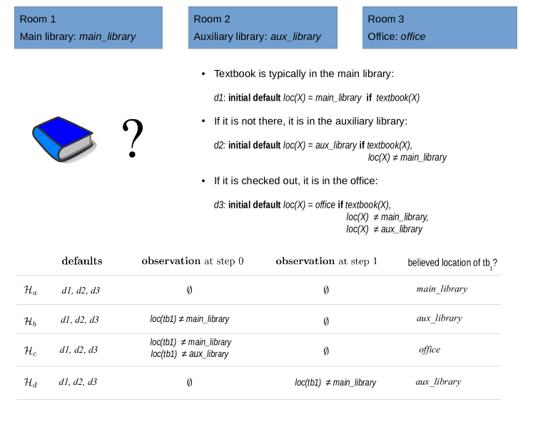
Figure 2: Illustration of the beliefs of a robot corresponding to the histories with the same initial state defaults, as described in Example 2 and Example 3.

To better understand the definition of histories with defaults, let us first recall the definition of a model for histories not containing defaults. In this case, a model of $\mathcal{H}^{n}$ is a path $M=\langle\sigma_{0},a_{0},\sigma_{1},\dots,\sigma_{n},a_{n}\rangle$ of ${\tau(\mathcal{D})}$ such that:

• $M$ satisfies every $obs(rob_{1},f(\bar{x})=y,i)\in\mathcal{H}^{n}$, i.e., for every such observation $(f(\bar{x})=y)\in\sigma_{i}$.

• $a_{i}=\{e:hpd(e,i)\in\mathcal{H}^{n}\}$.

In the presence of defaults, however, these conditions, though necessary, are not sufficient. Consider, for instance, history $\mathcal{H}_{a}$ from Example 2. Since it contains no actions or observations, these conditions are satisfied by any path $M=\langle\sigma_{0}\rangle$. However, $M$ is a model of $\mathcal{H}_{a}$ only if $\sigma_{0}$ contains $loc(tb1)=main\_library$. In general, to define the initial states of models of $\mathcal{H}^{n}$, we need to understand reasoning in the presence of defaults, along with their direct and indirect exceptions. The situation is similar to, but potentially more complex than, the definition of transitions of ${\tau(\mathcal{D})}$. To define the models of $\mathcal{H}^{n}$, we thus pursue an approach similar to that used to define the transitions of ${\tau(\mathcal{D})}$. Specifically, we define models of $\mathcal{H}^{n}$ in terms of answer sets of the logic program $\Pi(\mathcal{D},\mathcal{H})$ that axiomatizes the agent’s knowledge. However, due to the presence of indirect exceptions, our language of choice will be CR-Prolog, an extension of ASP well-suited for representing and reasoning with such knowledge. We begin by defining the program encoding both $\mathcal{D}$ and $\mathcal{H}$.

Definition 5.

[Program $\Pi(\mathcal{D},\mathcal{H})$]
Program $\Pi(\mathcal{D},\mathcal{H})$, encoding the system description $\mathcal{D}$ and history $\mathcal{H}$ of the domain, is obtained by changing the value of constant $n$ in $\Pi(\mathcal{D})$ from $1$ to the current step of $\mathcal{H}$ and adding to the resulting program:

• Observations and actions, i.e., Statements 21 and 23, from $\mathcal{H}$.

• Encoding of each default, i.e., for every default such as Statement 24 from $\mathcal{H}$, we add:

  $$val(f(\bar{x}),y,0)\leftarrow val(body(d(\bar{x})),0),$$ (30)

  $$\mbox{not }ab(d(\bar{x}))$$

  $$ab(d(\bar{x}))\stackrel{{\scriptstyle\,\,+}}{{\leftarrow}}val(body(d(\bar{x})),0)$$ (31)

  where Statement 30 is a simplified version of the standard CR-Prolog (or ASP) encoding of a default, and the relation $ab(d)$, read as default $d$ is abnormal, holds when default $d$ is not applicable. Statement 31 is a consistency restoring (CR) rule, which says that to restore consistency of the program one may refrain from applying default $d$. It is an axiom in CR-Prolog used to allow indirect exceptions to defaults—it is not used unless assuming $f(\bar{x})=y$ leads to a contradiction. For more details about CR rules, please see [23].

• Encoding of preference relations. If there are two or more defaults with preference relations, e.g., Statements 26-29, we first add the following:

  $$ab(D_{2})\leftarrow prefer(D_{1},D_{2}),$$ (32)

  $$val(body(D_{1}),0),$$

  $$\textrm{not }~{}~{}ab(D_{1})$$

  where $D_{1}$ and $D_{2}$ are defaults. Then, we add the following:

  $$prefer(D_{1},D_{3})\leftarrow prefer(D_{1},D_{2}),$$ (33)

  $$prefer(D_{2},D_{3})$$

  $$\neg prefer(D,D)$$ (34)

  Statement 32 prevents the applicability of a default if another (preferred) default is applicable. The other two axioms (Statements 33, 34) express transitivity and anti-symmetry of the preference relation.

• Rules for initial observations, i.e., for every basic fluent $f$ and its possible value $y$:

  $$val(f(\bar{x}),y,0) \leftarrow obs(rob_{1},f(\bar{x})=y,0)$$ (35)

  $$\neg val(f(\bar{x}),y,0) \leftarrow obs(rob_{1},f(\bar{x})\not=y,0)$$ (36)

  These axioms say that the initial observations are correct. Among other things they may be used to defeat the defaults of $\mathcal{H}$.

• Assignment of initial values to basic fluents that have not been defined by other means. Specifically, the initial value of a basic fluent not defined by a default is selected from the fluent’s range. To do so, for every initial state default (of the form of Statement 24) from $\mathcal{H}$:

  $$defined\_by\_default(f(\bar{x}))\leftarrow val(body(d(\bar{x})),0),$$ (37)

  $$\mbox{not }ab(d(\bar{x}))$$

  Then, for every basic fluent $f$:

  $$val(f(\bar{x}),y_{1},0)\mbox{ or }\dots\mbox{ or }val(f(\bar{x}),y_{n},0)\leftarrow\mbox{ not }defined\_by\_default(f(\bar{x}))$$ (38)

  where $\{y_{1},\dots,y_{n}\}$ are elements in the range of $f(\bar{x})$ not occurring in the head of any initial default of $\mathcal{H}$.

• A reality check [4]:

  $$\leftarrow val(F,Y_{1},I),~{}obs(rob_{1},F=Y_{2},I),~{}Y_{1}\not=Y_{2}$$ (39)

  which says that the value of a fluent predicted by our program shall not differ from its observed value.

• And a rule:

  $$occurs(A,I)\leftarrow hpd(A,I)$$ (40)

  which establishes the relation between relation $hpd$ of the language of recorded histories and relation $occurs$ used in the program. Recall that $occurs$ denotes both actual and hypothetical occurrences of actions, whereas $hpd$ indicates an actual occurrence.

This completes construction of the program.

We will also need the following terminology in the discussion below. Let $\mathcal{H}$ be a history of $\mathcal{D}$ and $AS$ be an answer set of $\Pi(\mathcal{D},\mathcal{H})$. We say that a sequence $M=\langle\sigma_{0},a_{0},\sigma_{1},\dots,\sigma_{n},a_{n}\rangle$ such that $\forall i\in[0,n]$:

• $\sigma_{i}=\{f=y:val(f,y,i)\in AS\}$,

• $a_{i}=\{e:hpd(e,i)\in AS\}$.

is induced by $AS$. Now we are ready to define semantics of $\mathcal{H}$.

Definition 6.

[Model]
A sequence $\langle\sigma_{0},a_{0},\sigma_{1},\dots,\sigma_{n},a_{n}\rangle$ induced by an answer set $AS$ of $\Pi(\mathcal{D},\mathcal{H})$ is called a model of $\mathcal{H}$ if it is a path of transition diagram ${\tau(\mathcal{D})}$.

Definition 7.

[Entailment]
A literal $l$ is true at step $i$ of a path $M=\langle\sigma_{0},a_{0},\sigma_{1},\dots,\sigma_{n},a_{n}\rangle$ of ${\tau(\mathcal{D})}$ if $l\in\sigma_{i}$. We say that $l$ is entailed by a history $\mathcal{H}$ of $\mathcal{D}$ if $l$ is true in all models of $\mathcal{H}$.

The following proposition shows that for well-founded system descriptions this definition can be simplified.

Proposition 1.

[Answer sets of $\Pi(\mathcal{D},\mathcal{H})$ and paths of ${\tau(\mathcal{D})}$]
If $\mathcal{D}$ is a well-founded system description and $\mathcal{H}$ is its recorded history, then every sequence induced by an answer set of $\Pi(\mathcal{D},\mathcal{H})$ is a model of $\mathcal{H}$.

The proof of this proposition is in Appendix A. Next, we look at some examples of histories with defaults.

Example 3.

[Example 2 revisited]
Let us revisit the histories described in Example 2 and show how models of system descriptions from this example can be computed using our axiomatization $\Pi(\mathcal{D},\mathcal{H})$ of models of a recorded history. We see that models of $\mathcal{H}_{a}$ are of the form $\langle\sigma_{0}\rangle$ where $\sigma_{0}$ is a state of the system containing $\{loc(tb_{1})=main\_library\}$. Since $textbook(tb_{1})$ is a static relation, it is true in every state of the system. The axiom encoding default $d_{1}$ (Statement 30) is not blocked by a CR rule (Statement 31) or a preference rule (Statement 32), and the program entails $val(loc(tb_{1}),main\_library,0)$. Thus, $\{loc(tb_{1})=main\_library\}\in\sigma_{0}$.

Now consider $\mathcal{H}_{b}$ containing $obs(rob_{1},loc(tb_{1})\not=main\_library,0)$. Based on rules for initial observations (Statement 36) we have $\neg val(loc(tb_{1}),main\_library,0)$ which contradicts the first default. The corresponding CR-rule (Statement 31) restores consistency by assuming $ab(d_{1})$, making default $d_{1}$ inapplicable. Default $d_{2}(tb_{1})$, which used to be blocked by a preference rule (i.e., $prefer(d_{1}(tb_{1}),d_{2}(tb_{1}))$), becomes unblocked and we conclude that $val(loc(tb_{1}),aux\_library,0)$. Models of $\mathcal{H}_{b}$ are states of $\tau(\mathcal{D})$ that contain $\{loc(tb_{1})=aux\_library\}$. A similar argument can be used to compute the models of $\mathcal{H}_{c}$ in Example 2.

Recall that the last history, $\mathcal{H}_{d}$, is slightly different. It contains $obs(rob_{1},loc(tb_{1})\not=main\_library,1)$. The current step of $\mathcal{H}_{d}$ is $1$ and its models are of the form $\langle\sigma_{0},a,\sigma_{1}\rangle$. Since $\Pi(\mathcal{D},\mathcal{H}_{d})$ has no rules with an action in the head, $a=\{\ \}$. Based on default $d_{1}$, $\{loc(tb_{1})=main\_library\}$ should belong to state $\sigma_{0}$. However, if this were true, $\{loc(tb_{1})=main\_library\}$ would belong to $\sigma_{1}$ by inertia, which contradicts the observation and the reality check axiom creates an inconsistency. This inconsistency is resolved by the corresponding CR-rule (Statement 31) by assuming $ab(d_{1})$ in the initial state (i.e., at time $0$). Now the default $d_{2}$ is activated and the reasoner concludes $\{loc(tb_{1})=aux\_library\}$ at time step $0$ and (by inertia) at time step $1$.

To illustrate the use of axioms governing the initial value of a basic fluent not defined by a default (Statements 37 and 38), consider history $\mathcal{H}_{e}$ in which observations at step $1$ establish that textbook $tb_{1}$ is not in any of the default locations. An argument similar to that used for $\mathcal{H}_{d}$ would allow the reasoner to conclude $ab(d_{1}(tb_{1}))$, $ab(d_{2}(tb_{1}))$, and $ab(d_{3}(tb_{1}))$, and $defined\_by\_default(loc(tb_{1}))$ can not be derived. Statement 38 is now used to allow a choice between the four locations that form the range of the $loc()$ function. The first three are eliminated by observations at step $1$ and we thus conclude $val(loc(tb_{1}),kitchen,0)$, i.e., $\{loc(tb_{1})=kitchen\}\in\sigma_{1}$. Note that if the domain included other available locations, we would have additional models of history $\mathcal{H}_{e}$.

Example 4.

[Examples of models of history]
As further examples of models of history, consider a system description $\mathcal{D}_{a}$ with basic boolean fluents $f$ and $g$ (and no actions), and a history $\mathcal{H}_{a}$ consisting of:

$${\bf initial\ default}\ \neg g\ {\bf if}\ f$$

The paths of this history consist of states without any transitions. Using axiom in Statement 38, we see that $\{f,\neg g\}$, $\{\neg f,g\}$, and $\{\neg f,\neg g\}$ are models of $\langle\mathcal{D}_{a},\mathcal{H}_{a}\rangle$ and $\sigma=\{f,g\}$ is not. The latter is not surprising since even though $\sigma$ may be physically possible, the agent, relying on the default, will not consider $\sigma$ to be compatible with the default since the history gives no evidence that the default should be violated. If, however, the agent were to record an observation $obs(rob_{1},g,0)$, the only states compatible with the resulting history ${\mathcal{H}}_{b}$ would be $\{f,g\}$ and $\{\neg f,g\}$.)

Next, we expand our system description $\mathcal{D}_{a}$ by a basic fluent $h$ and a state constraint:

$$h\ {\bf if}\ \neg g$$

In this case, to compute models of a history ${\mathcal{H}}_{c}$ of a system $\mathcal{D}_{b}$, where ${\mathcal{H}}_{c}$ consists of the default in $\mathcal{H}_{a}$ and an observation $obs(rob_{1},\neg h,0)$, we need CR rules. The models are $\{f,\neg h,g\}$ and $\{\neg f,\neg h,g\}$.

Next, consider a system description $\mathcal{D}_{c}$ with basic fluents $f$, $g$, and $h$, the initial-state default, and an action $a$ with the following causal law:

$$a\ {\bf causes}\ h\ {\bf if}\ \neg g$$

and a history ${\mathcal{H}}_{d}$ consisting of $obs(rob_{1},f,0)$, $hpd(a,0)$; $\langle\{f,\neg g,h\},a,\{f,\neg g,h\}\rangle$ and $\langle\{f,\neg g,\neg h\},a,\{f,\neg g,h\}\rangle$ are the two models of ${\mathcal{H}}_{d}$. Finally, history ${\mathcal{H}}_{e}$ obtained by adding $obs(rob_{1},\neg h,1)$ to ${\mathcal{H}}_{d}$ has a single model $\langle\{f,g,\neg h\},a,\{f,g,h\}\rangle$. The new observation is an indirect exception to the initial default, which is resolved by the corresponding CR rule.

5.3 Reasoning

The main reasoning task of an agent with a high level deterministic system description $\mathcal{D}$ and history $\mathcal{H}$ is to find a plan (i.e., a sequence of actions) that would allow it to achieve goal $G$. We assume that the length of this sequence is limited by some number $h$ referred to as the planning horizon. This is a generalization of a classical planning problem in which the history consists of a collection of atoms which serves as a complete description of the initial state. If history $\mathcal{H}$ has exactly one model, the situation is not very different from classical planning. The agent believes that the system is currently in some unique state $\sigma_{n}$—this state can be found using Proposition 1 that reduces the task of computing the model of $\mathcal{H}$ to computing the answer set of $\Pi(\mathcal{D},\mathcal{H})$. Finding a plan is thus equivalent to solving a classical planning problem $\mathcal{P}_{c}$, i.e., finding a sequence of actions of length not exceeding $h$, which leads the agent from an initial state $\sigma$ to a state satisfying $G$. The ASP-based solution of this planning problem can be traced back to work described in [14, 63]. Also see program $plan(\mathcal{P}_{c},h)$ and Proposition 9.1.1 in Section 9.1 of [23], which establish the relationship between answer sets of this program and solutions of $\mathcal{P}_{c}$, and can be used to find a plan to achieve the desired goal. A more subtle situation arises when $\mathcal{H}$ has multiple models. Since there are now multiple possible current states, we can either search for a possible plan, i.e. a plan leading to $G$ from at least one of the possible current states, or for a conformant plan, i.e., a plan that can achieve $G$ independent of the current state. In this paper, we only focus on the first option.

Definition 8.

[Planning Problem]
We define a planning problem $\mathcal{P}$ as a tuple $(\mathcal{D},\mathcal{H},h,G)$ consisting of system description $\mathcal{D}$, history $\mathcal{H}$, planning horizon $h$ and a goal $G$. A sequence $\langle a_{0},\dots,a_{k-1}\rangle$ is called a solution of $\mathcal{P}$ if there is a state $\sigma$ such that:

• $\sigma$ is the current state of some model $M$ of $\mathcal{H}$; and

• $\langle a_{0},\dots,a_{k-1}\rangle$ is a solution of classical planning problem $\mathcal{P}_{c}=(\mathcal{D},\sigma,G)$ with horizon $h$.

To find a solution of $\mathcal{P}$ we consider:

• CR-Prolog program $Diag=_{def}\Pi^{n}(\mathcal{D},\mathcal{H})$ with maximum time step $n$ where $n$ is the current step of $\mathcal{H}$.

• ASP program $Classical\_plan$ consisting of:

  1. $\Pi^{[n..n+h]}(\mathcal{D})$ obtained from $\Pi(\mathcal{D})$ by setting $max\_step$ to $n+h$ and sort $step$ to $(n,max\_step)$.

  2. Encoding of the goal $f(\bar{x})=y$ by the rule:

     $$goal(I)\leftarrow val(f(\bar{x}),y,I)$$

  3. Simple planning module, $PM$, obtained from that in Section $9.1$ of [23] (see statements on page 194) by letting time step variable $I$ range between $n$ and $n+h$.

• Diagnoses Preserving Constraint (DPC):

  $$\leftarrow Y=count\{X:ab(X)\},Y>m$$

  where $m$ is the size of abductive support of $Diag$. For any program $\Pi$, if $\Pi^{reg}$ is the set of all regular rules of $\Pi$ and $\alpha(R)$ is the set of regular rules obtained by replacing $\stackrel{{\scriptstyle\,\,+}}{{\leftarrow}}$ by $\leftarrow$ in each CR rule in $R$, a cardinality-minimal set of CR rules such that $\Pi(R)=_{def}\Pi^{reg}\cup\alpha(R)$ is consistent, is called an abductive support of $\Pi$.

Proposition 2 can be used to reduce finding the solutions of the planning problem $\mathcal{P}$ to:

1. Computing the size, $m$, of an abductive support of $Diag$.

2. Computing answer sets of CR-Prolog program:

   $$Plan=Diag\cup Classical\_plan\cup\{DPC\}$$

Based on Proposition 1, the first task of finding the abductive support of $Diag$ can be accomplished by computing a model of:

$$Diag\cup\{size(Y)\leftarrow count\{X:ab(X)\}=Y\}$$

and displaying atom $size(m)$ from this model. The second task of reducing planning to compute answer sets is based on the following proposition that is analogous to Proposition $9.1.1$ in Section $9.1$ of [23].

Proposition 2.

[Reducing planning to computing answer sets]
Let $\mathcal{P}=(\mathcal{D},\mathcal{H},h,G)$ be a planning problem with a well-founded, deterministic system description $\mathcal{D}$. A sequence $\langle a_{0},\dots,a_{k-1}\rangle$ where $k<h$ is a solution of $\mathcal{P}$ iff there is an answer set $A$ of $Plan$ such that:

1. For any $n<i\leq n+k$, $occurs(a_{i},i-1)\in A$,

2. $A$ contains no other atoms of the form $occur(*,i)$ with $i\geq n$.

The proof of this proposition is provided in Appendix B. Similar to classical planning, it is possible to find plans for our planning problem that contain irrelevant, unnecessary actions. We can avoid this problem by asking the planner to search for plans of increasing length, starting with plans of length $1$, until a plan is found. There are other ways to find minimum-length plans, but we do not discuss them here.

6 Logician’s Domain Representation

We are now ready for the first step of our design methodology (see Section 4), which is to provide a coarse-resolution description of the robot’s domain in $\mathcal{AL}_{d}$ along with a description of the initial state—we re-state this step as specifying the transition diagram of the logician.

1. Specify the transition diagram, $\tau_{H}$, which will be used by the logician for coarse-resolution reasoning, including planning and diagnostics.

This step is accomplished by providing the signature and $\mathcal{AL}_{d}$ axioms of system description $\mathcal{D}_{H}$ defining this diagram. We will use standard techniques for representing knowledge in action languages, e.g., [23]. We illustrate this process by describing the domain representation for the office domain introduced in Example 1.

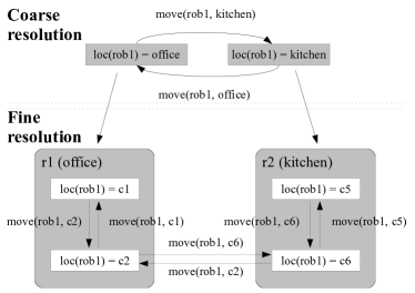
(a) Some state transitions

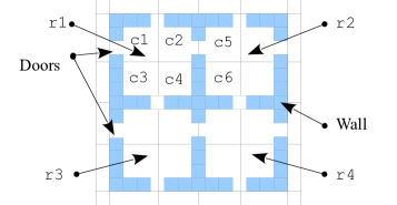
(b) Different resolutions

Figure 3: (a) Illustration of state transitions for specific $move$ actions in our illustrative (office) domain, viewed at coarse resolution and at fine resolution; and (b) A closer look at specific places brings into focus the corresponding rooms and grid cells in those rooms.

Example 5.

[Logician’s domain representation]
The system description $\mathcal{D}_{H}$ of the domain in Example 1 consists of a sorted signature ($\Sigma_{H}$) and axioms describing the transition diagram $\tau_{H}$. $\Sigma_{H}$ defines the names of objects and functions available for use by the logician. Building on the description in Example 1, $\Sigma_{H}$ has an ontology of sorts, i.e., sorts such as $place$, $thing$, $robot$, and $object$, which are arranged hierarchically, e.g., $object$ and $robot$ are subsorts of $thing$, and $textbook$ and $cup$ are subsorts of $object$. The statics include a relation $next\_to:place\times place\rightarrow boolean$, which holds iff two places are next to each other. This domain has two basic fluents that are subject to the laws of inertia: $loc:thing\rightarrow place$, $in\_hand:robot\times object\rightarrow boolean$. For instance, the $loc(Th)=Pl$ if thing $Th$ is located at place $Pl$, and the value of $in\_hand(R,Ob)$ is $true$ if robot $R$ is holding object $Ob$. In this domain, the basic fluents are observable.

The domain has three actions: $move(robot,place)$, $grasp(robot,object)$, and $putdown(robot,object)$. The domain dynamics are defined using axioms that consist of causal laws such as:

$$move(R,Pl)~{}~{}\mathbf{causes}~{}~{}loc(R)=Pl$$ (41a)

$$grasp(R,Ob)~{}~{}\mathbf{causes}~{}~{}in\_hand(R,Ob)$$ (41b)

$$putdown(R,Ob)~{}~{}\mathbf{causes}~{}~{}\neg in\_hand(R,Ob)$$ (41c)

state constraints such as:

$$loc(Ob)=Pl~{}~{}\mathbf{if}~{}~{}loc(R)=Pl,~{}~{}in\_hand(R,Ob)$$ (42a)

$$next\_to(P1,P2)~{}~{}\mathbf{if}~{}~{}next\_to(P2,P1)$$ (42b)

and executability conditions such as:

$$\mathbf{impossible}~{}~{}move(R,Pl)~{}~{}\mathbf{if}~{}~{}loc(R)=Pl$$ (43a)

$$\mathbf{impossible}~{}~{}move(R,Pl_{2})~{}~{}\mathbf{if}~{}~{}loc(R)=Pl_{1},~{}\neg next\_to(Pl_{1},Pl_{2})$$ (43b)

$$\mathbf{impossible}~{}~{}A_{1},~{}A_{2}~{}~{}\mathbf{if}~{}~{}A_{1}\neq A_{2}$$ (43c)

$$\mathbf{impossible}~{}~{}grasp(R,Ob)~{}~{}\mathbf{if}~{}~{}loc(R)=Pl_{1},~{}loc(Ob)=Pl_{2},~{}Pl_{1}\neq Pl_{2}$$ (43d)

$$\mathbf{impossible}~{}~{}grasp(R,Ob)~{}~{}\mathbf{if}~{}~{}in\_hand(R,Ob)$$ (43e)

$$\mathbf{impossible}~{}~{}putdown(R,Ob)~{}~{}\mathbf{if}~{}~{}\neg in\_hand(R,Ob)$$ (43f)

The part of $\Sigma_{H}$ described so far, the sort hierarchy and the signatures of functions, is unlikely to undergo substantial changes for any given domain. However, the last step in the constructions of $\Sigma_{H}$ is likely to undergo more frequent revisions—it populates the sorts of the hierarchy with specific objects; e.g $robot=\{rob_{1}\}$, $place=\{r_{1},\dots,r_{n}\}$ where $r$s are rooms, $textbook=\{tb_{1},\dots\,tb_{m}\}$, $kitchenware=\{cup_{1},cup_{2},plate_{1},plate_{2}\}$ etc. Ground instances of the axioms are obtained by replacing variables by ground terms from the corresponding sorts.

The transition diagram $\tau_{H}$ described by $\mathcal{D}_{H}$ is too large to depict in a picture. The top part of Figure 3(a) shows the transitions of $\tau_{H}$ corresponding to a $move$ between two places. The only fluent shown there is the location of the robot $rob_{1}$—the values of other fluents remain unchanged and are not shown here. The actions of this coarse-resolution transition diagram $\tau_{H}$ of the logician, as described above, are assumed to be deterministic. Also, the values of coarse-resolution fluents are assumed to be known at each time step. These assumptions allow the robot to do fast, tentative planning and diagnostics necessary for achieving its assigned goals.

The domain representation described above should ideally be tested extensively. This can be done by including various recorded histories of the domain, which may include histories with prioritized defaults (Example 2), and using the resulting programs to solve various reasoning tasks.

The logician’s model of the world thus consists of the system description $\mathcal{D}_{H}$ (Example 5), and recorded history $\mathcal{H}$ of initial state defaults (Example 2), actions, and observations. The logician achieves any given goal by first translating the model (of the world) to an ASP program $\Pi(\mathcal{D}_{H},\mathcal{H})$, as described in Sections 5.1, 5.2, and expanding it to include the definition of goal and suitable axioms, as described at the end of Section 5.3. For planning and diagnostics, this program is passed to an ASP solver—we use SPARC, which expands CR-Prolog and provides explicit constructs to specify objects, relations, and their sorts  [2]. Please see example4.sp at https://github.com/mhnsrdhrn/refine-arch for the SPARC version of the complete program. The solver returns the answer set of this program. Atoms of the form:

$$occurs(action,step)$$

belonging to this answer set, e.g., $occurs(a_{1},1),\ldots,occurs(a_{n},n)$, represent the shortest plan, i.e., the shortest sequence of abstract actions for achieving the logician’s goal. Prior research results in the theory of action languages and ASP ensure that the plan is provably correct [23]. In a similar manner, suitable atoms in the answer set can be used for diagnostics, e.g., to explain unexpected observations by triggering suitable CR rules.

7 Refinement, Zoom and Randomization

For any given goal, each abstract action in the plan created by reasoning with the coarse-resolution domain representation is implemented as a sequence of concrete actions by the statistician. To do so, the robot probabilistically reasons about the part of the fine-resolution transition diagram relevant to the abstract action to be executed. This section defines refinement, randomization, and the zoom operation, which are necessary to build the fine-resolution models for such probabilistic reasoning, along with the corresponding steps of the design methodology.

7.1 Refinement

Although the representation of a domain used by a logician specifies fluents with observable values and assumes that all of its actions are executable, the robot may not be able to directly make some of these observations or directly execute some of these actions. For instance, a robot may not have the physical capability to directly observe if it is located in a given room, or to move in a single step from one room to another. We refer to such actions that cannot be executed directly and fluents that cannot be observed directly as abstract; actions that can be executed and fluents that can be observed directly are, on the other hand, referred to as concrete. The second step of the design methodology (see Section 4) requires the designer to refine the coarse-resolution transition diagram $\tau_{H}$ of the domain by including information needed to execute the abstract actions suggested by a logician, and to observe values of relevant abstract statics and fluents. This new transition diagram $\tau_{L}$ defined by system description $\mathcal{D}_{L}$, is called the refinement of $\tau_{H}$. Its construction may be imagined as the designer taking a closer look at the domain through a magnifying lens. Looking at objects of a sort $s$ of $\Sigma_{H}$ at such finer resolution may lead to the discovery of parts of these objects and their attributes previously abstracted out by the designer. Instead of being a single entity, a room may be revealed to be a collection of cells with some of them located next to each other, a cup may be revealed to have parts such as handle and base, etc. If such a discovery happens, the sort $s$ and its objects will be said to have been magnified, and the newly discovered parts are called the components of the corresponding objects. In a similar manner, a function $f:s_{1},\dots,s_{n}\rightarrow s_{0}$ from $\Sigma_{H}$ is affected by the increased resolution or magnified if:

• It is an abstract action or fluent and hence can not be executed or observed directly by robots; and

• At least one of $s_{0},\dots,s_{n}$ is magnified.

In the signature $\Sigma_{L}$ of the fine-resolution model $\tau_{L}$, the newly discovered components of objects from a sort $s$ of $\Sigma_{H}$ form a new sort $s^{*}$, which is called the fine-resolution counterpart of $s$. For instance, in our example domain, $place^{*}$, which is a collection of grid cells $\{c_{1},\ldots,c_{n}\}$, is the fine-resolution counterpart of $place$, which is a collection of rooms, and $object^{*}$ may be the collection of parts of cups. A vector $\bar{s}^{*}$ is a fine-resolution counterpart of $\bar{s}$ with respect to magnified sorts $s_{i_{1}},\dots,s_{i_{k}}$ (with $k>0$) if it is obtained by replacing $s_{i_{1}},\dots,s_{i_{k}}$ by $s^{*}_{i_{1}},\dots,s^{*}_{i_{k}}$. Every element $\bar{x}$ of $\bar{s}^{*}$ is obtained from the unique element $\bar{u}$ of $\bar{s}$ by replacing $u_{i_{1}},\dots,u_{i_{k}}$ from $s_{i_{1}},\dots,s_{i_{k}}$ by their components. We say that $\bar{u}$ is the generator of $\bar{x}$ in $\bar{s}^{*}$ and $\bar{x}$ is a fine-resolution counterpart of $\bar{u}$. A function $f^{*}$ with signature $\bar{s}^{*}$ is called the fine-resolution counterpart of a magnified function $f$ with respect to $\langle s_{i_{1}},\dots,s_{i_{k}}\rangle$ if for every $\langle u_{1},\dots,u_{n},v\rangle\in\bar{s}$, $f(u_{1},\dots,u_{n})=v$ iff there is a fine-resolution counterpart $\langle x_{1},\dots,x_{n},y\rangle\in\bar{s}^{*}$ of $\langle u_{1},\dots,u_{n},v\rangle$ such that $f^{*}(x_{1},\dots,x_{n})=y$. For instance, fluents $loc^{*}:thing\rightarrow place^{*}$, $loc^{*}:object^{*}\rightarrow place^{*}$, and $loc^{*}:object^{*}\rightarrow place$ are fine-resolution counterparts of $loc$ with respect to $\langle place\rangle$, $\langle object,place\rangle$ and $\langle object\rangle$ respectively; and action $move^{*}:robot\times place^{*}\rightarrow boolean$ is the fine-resolution counterpart of $move:robot\times place\rightarrow boolean$ with respect to $place$. In many interesting domains, some fine-resolution counterparts can be used to execute or observe magnified functions of $\Sigma_{H}$, e.g., an abstract action of moving to a neighbouring room can be executed by a series of moves to neighbouring cells. We describe other such examples later in this section.

We now define the refinement of a transition diagram. We do so in two steps. We first define a notion of weak refinement that does not consider the robot’s ability to observe the values of domain fluents. We then introduce our theory of observations, and define a notion of strong refinement (or simply refinement) that includes the robot’s ability to observe the values of domain fluents.

7.1.1 Weak Refinement

We introduce some terminology used in the definition below. Let signature $\Sigma_{1}$ be a subsignature of signature $\Sigma_{2}$ and let $\sigma_{1}$ and $\sigma_{2}$ be interpretations over these signatures. We say that $\sigma_{2}$ is an extension of $\sigma_{1}$ if $\sigma_{2}|_{\Sigma_{1}}=\sigma_{1}$.

Definition 9.

[Weak refinement of $\tau_{H}$]
A transition diagram $\tau_{L}$ over $\Sigma_{L}$ is called a weak refinement of $\tau_{H}$ if:

1. For every state $\sigma^{\diamond}$ of $\tau_{L}$, the collection $\sigma^{\diamond}|_{\Sigma_{H}}$ of atoms of $\sigma^{\diamond}$ formed by symbols from $\Sigma_{H}$ is a state of $\tau_{H}$.

2. For every state $\sigma$ of $\tau_{H}$, there is a state $\sigma^{\diamond}$ of $\tau_{L}$ such that $\sigma^{\diamond}$ is an extension of $\sigma$.

3. For every transition $T=\langle\sigma_{1},a^{H},\sigma_{2}\rangle$ of $\tau_{H}$, if $\sigma^{\diamond}_{1}$ and $\sigma^{\diamond}_{2}$ are extensions of $\sigma_{1}$ and $\sigma_{2}$ respectively, then there is a path $P$ in $\tau_{L}$ from $\sigma^{\diamond}_{1}$ to $\sigma^{\diamond}_{2}$ such that:

   • actions of $P$ are concrete, i.e., directly executable by robots; and

   • $P$ is pertinent to $T$, i.e., all states of $P$ are extensions of $\sigma_{1}$ or $\sigma_{2}$.

We are now ready to construct the fine-resolution system description $\mathcal{D}_{L,nobs}$ corresponding to the coarse-resolution system description $\mathcal{D}_{H}$ for our running example (Example 5). This construction does not consider the robot’s ability to observe the values of domain fluents (hence the subscript “nobs”). We start with the case in which the only magnified sort in $\Sigma_{H}$ is $place$. The signature $\Sigma_{L}$ will thus contain three fine-resolution counterparts of functions from $\Sigma_{H}$: (i) basic fluent $loc^{*}:thing\rightarrow place^{*}$; (ii) action $move^{*}:robot\rightarrow place^{*}$; and (iii) defined static $next\_to^{*}:place^{*}\times place^{*}\rightarrow boolean$. We assume that $loc^{*}$ and $next\_to^{*}$ are directly observable and $move^{*}$ is executable by the robot. These functions ensure indirect observability of $loc$ and $next\_to$ and indirect executability of $move$. Although this construction is domain dependent, the approach is applicable to other domains.

2. Constructing the fine-resolution system description $\mathcal{D}_{L}$ corresponding to the coarse-resolution system description $\mathcal{D}_{H}$. (a) Constructing $\mathcal{D}_{L,nobs}$.

To construct signature $\Sigma_{L,nobs}$:

1. Preserve all elements of signature $\Sigma_{H}$.

   In our running example, this includes sorts $thing$, $place$, $robot$, $cup$ etc, object constants $rob_{1}$, $kitchen$, $of\!\!fice$, $cup_{1}$, $tb_{1}$ etc, static $next\_to(place,place)$, fluents $loc:thing\to place$ and $in\_hand:robot\times place\rightarrow boolean$, and actions $move(robot,place)$, $grasp(robot,object)$ and $putdown(robot,object)$.

2. Introduce a new sort $s^{*}$ for every sort $s$ of $\Sigma_{H}$ that is magnified by the increase in resolution, with $s^{*}$ consisting of components of elements of $s$. Add $s^{*}$ to the sort hierarchy as a sibling of $s$. Also, for each abstract function $f$ magnified by the increase in resolution, introduce appropriate fine-resolution counterparts that support the execution or observation of $f$ at the fine-resolution.

   In our example, we introduce the sort $place^{*}$ as the fine-resolution counterpart of $place$, and object constants $c_{1},\ldots,c_{n}$ of sort $place^{*}$ that are grid cells; no new sort is introduced for the sort $object$. Also, $\Sigma_{L,nobs}$ includes new static relation $next\_to^{*}(place^{*},place^{*})$, new fluent $loc^{*}:thing\to place^{*}$, and new action $move^{*}(robot,place^{*})$, but no new symbols corresponding to $in\_hand$ or $grasp$.

3. Introduce static relations $component(O^{*},O)$, which hold iff object $O^{*}$ of sort $s^{*}$ is a component of magnified object $O$ of sort $s$ of $\Sigma_{H}$. These relations are domain dependent and need to be provided by the designer.

   Continuing with our running example, we introduce the static relation:

   $$component:place^{*}\times place\rightarrow boolean$$

   where $component(c,r)$ is true iff cell $c$ is part of room $r$.

Next, to construct the axioms of $\mathcal{D}_{L,nobs}$:

1. For each axiom of $\mathcal{D}_{H}$, if it contains any abstract functions, replace them by their fine-resolution counterparts and make these functions’ variables range over appropriate sorts required by these counterparts.

   In our running example, all occurrences of the functions $loc:thing\rightarrow place$, $next\_to(place,place)$, and $move(robot,place)$ in the axioms of $\mathcal{D}_{H}$ are replaced by $loc:thing\rightarrow place^{*}$, $next\_to^{*}(place^{*},place^{*})$ and $move^{*}(robot,place^{*})$ respectively. At the same time, $in\_hand(robot,object)$, $grasp(robot,object)$, and $putdown(robot,object)$ are functions that remain unchanged. This results in $\mathcal{D}_{L,nobs}$ having causal laws:

   $$move^{*}(R,C)~{}~{}\mathbf{causes}~{}~{}loc^{*}(R)=C$$ (44a)

   $$grasp(R,O)~{}~{}\mathbf{causes}~{}~{}in\_hand(R,O)$$ (44b)

   $$putdown(R,O)~{}~{}\mathbf{causes}~{}~{}\neg in\_hand(R,O)$$ (44c)

   state constraints:

   $$loc^{*}(O)=C~{}~{}\mathbf{if}~{}~{}loc^{*}(R)=C,~{}in\_hand(R,O)$$ (45a)

   $$next\_to^{*}(C_{2},C_{1})~{}~{}\mathbf{if}~{}~{}next\_to^{*}(C_{1},C_{2})$$ (45b)

   and executability conditions such as:

   $$\mathbf{impossible}~{}~{}move^{*}(R,C)~{}~{}\mathbf{if}~{}~{}loc^{*}(R)=C$$ (46a)

   $$\mathbf{impossible}~{}~{}move^{*}(R,C_{2})~{}~{}\mathbf{if}~{}~{}loc^{*}(R)=C_{1},~{}\neg next\_to^{*}(C_{1},C_{2})$$ (46b)

   $$\mathbf{impossible}~{}~{}grasp(R,O)~{}~{}\mathbf{if}~{}~{}loc^{*}(R)=C_{1},~{}loc^{*}(O)=C_{2},~{}C_{1}\neq C_{2}$$ (46c)

   $$\mathbf{impossible}~{}~{}putdown(R,O)~{}~{}\mathbf{if}~{}~{}\neg in\_hand(R,O)$$ (46d)

   where $C$, $C_{1}$, and $C_{2}$ are grid cells.

2. Introduce bridge axioms, i.e., axioms relating the coarse-resolution functions and their fine-resolution counterparts. These axioms have the form:

   $$f(X_{1},\dots,X_{m})=Y~{}~{}\mathbf{if}~{}~{} component(C_{1},X_{1}),~{}\ldots~{},~{}component(C_{m},X_{m}),~{}component(C,Y),$$ (47)

   $$f^{*}(C_{1},\dots,C_{m})=C$$

   In our running example, we have:

   $$loc(Th)=P~{}~{}{\bf if}~{}~{}component(C,P),~{}loc^{*}(Th)=C$$ (48a)

   $$next\_to(P_{1},P_{2})~{}~{}\mathbf{if}~{}~{}component(C_{1},P_{1}),~{}component(C_{2},P_{2}),~{}next\_to^{*}(C_{1},C_{2})$$ (48b)

   These axioms are domain dependent and need to be provided by the designer.

This completes the construction of $\mathcal{D}_{L,nobs}$ for our running example.

To illustrate the robot’s reasoning with $\mathcal{D}_{L,nobs}$, consider a fine-resolution state $\delta_{1}$ in which the robot is in cell $c_{2}$ of the $of\!\!fice$, i.e., $(loc^{*}(rob_{1})=c_{2})\in\delta_{1}$. If $\delta_{1}$ is a fine-resolution counterpart of a coarse-resolution state $\sigma_{1}$, then $(loc(rob_{1})=of\!\!fice)\in\sigma_{1}$ because the bridge axiom in Statement 48(a) infers $loc(rob_{1})=of\!\!fice$ from $loc^{*}(rob_{1})=c_{2}$. Next, consider the robot’s move from $\delta_{1}$, with book $tb_{1}$ in its hand, to a cell $c_{5}$ in the $kitchen$. If $\delta_{2}$ is the resultant fine-resolution state, $(loc^{*}(rob_{1})=c_{5})\in\delta_{2}$ based on Statement 44(a), and $(loc^{*}(tb_{1})=c_{5})\in\delta_{2}$ based on Statement 45(a). Now, if $\delta_{2}$ is a fine-resolution counterpart of a coarse-resolution state $\sigma_{2}$, then based on the bridge axiom in Statement 48(a), $(loc(rob_{1})=kitchen)\in\sigma_{2}$ and $(loc(tb_{1})=kitchen)\in\sigma_{2}$.

The following proposition says that $\mathcal{D}_{L,nobs}$ as constructed above is a weak refinement of $\mathcal{D}_{H}$.

Proposition 3.

[Weak Refinement]
Let $\mathcal{D}_{H}$ and $\mathcal{D}_{L,nobs}$ be the coarse-resolution and fine-resolution system descriptions from our running example. Then $\tau_{L,nobs}$ is a weak refinement of $\tau_{H}$.

The proof of this proposition is in Appendix C. Although the statement of the proposition and its proof are provided here for our example domain, this approach can also be used to construct $\mathcal{D}_{L,nobs}$ and establish weak refinement in many other robotics domains.

7.1.2 Theory of Observations

The definition of weak refinement does not take into account the robot’s ability to observe the values of fluents in the domain. This ability to observe plays an important role in updating beliefs and monitoring the results of action execution in the fine-resolution. Recall that abstract fluents and statics are indirectly observable and the concrete fluents and statics are directly observable. In our running example, the observation of a thing being in a room can be inferred by checking if the thing can be observed in some cell of this room. Also, the robot has to monitor its movement between a series of neighboring cells when it attempts to execute the abstract action of moving to a neighbouring room. In this section, we introduce a Theory of Observations that supports this ability. This theory is used in conjunction with any given system description $\mathcal{D}_{L,nobs}$ as follows.

1. Expand $\Sigma_{L,nobs}$:

   • For every directly observable function $f$, include the actions:

     $$test_{f}:robot\times dom(f)\times range(f)\rightarrow boolean$$

     For $y\in range(f)$, this action checks if the value of $f$ is $y$ in a given state. For readability, we will sometimes abuse notation and write this action as $test(R,F,Y)$.

     In our example domain, we include an action such as $test_{loc^{*}}(rob_{1},O,C)$ for the robot to check if the location of an object $O$ is a particular cell $C$.

   • For every (directly or indirectly) observable function $f$, include the basic knowledge fluent:

     $$observed_{f}:robot\times dom(f)\times range(f)\rightarrow\{true,false,undet\}$$

     where the outcome undet stands for “undetermined”. For every $x\in dom(f)$ and $y\in range(f)$, the value of $observed_{f}(rob_{1},x,y)$ is the result of the most recent execution of action $test_{f}(rob_{1},x,y)$. Initially, the value is set to undet. After $test_{f}(rob_{1},x,y)$ is executed at least once, the value becomes (and remains) boolean. It is true if the most recent test returned true and false otherwise.

     In our example domain, we have basic knowledge fluents such as:

     $$observed_{loc^{*}}(rob_{1},O,C)$$

     $$observed_{loc}(rob_{1},O,P)$$

   • For every indirectly observable function $f$, introduce observation-related, domain-dependent defined fluent, as described in Statement 1:

     $$observable_{f}:robot\times dom(f)\times range(f)\to boolean$$

     Also, for every directly observable domain function $f$, introduce observation-related, domain-dependent defined fluents:

     $$can\_be\_observed_{f}:robot\times dom(f)\times range(f)\rightarrow boolean$$ (49)

     These fluents will be used to describe conditions for the observability of the corresponding functions. These domain dependent fluents need to be defined by the designer.

2. Expand axioms of $\mathcal{D}_{L,nobs}$ by axioms that model the robot’s ability to observe.

   • Introduce causal laws to describe the effect of the knowledge-producing action $test_{f^{*}}(R,\bar{X},Y)$ on the fine-resolution basic fluent $f^{*}$:

     $$test_{f^{*}}(R,\bar{X},Y) ~{}~{}\mathbf{causes}~{}~{}observed_{f^{*}}(R,\bar{X},Y)=true~{}~{}{\bf if}~{}~{}f^{*}(\bar{X})=Y$$ (50)

     $$test_{f^{*}}(R,\bar{X},Y) ~{}~{}\mathbf{causes}~{}~{}observed_{f^{*}}(R,\bar{X},Y)=false~{}~{}{\bf if}~{}~{}f^{*}(\bar{X})=Y_{1},~{}Y_{1}\not=Y$$

     Also introduce the executability condition:

     $${\bf impossible}~{}~{}test_{f^{*}}(R,\bar{X},Y)~{}~{}{\bf if}~{}~{}\lnot can\_be\_observed_{f^{*}}(R,\bar{X},Y)$$ (51)

     where $\bar{X}$ represents the domain of $f^{*}$.

     In our running example, if robot $rob_{1}$ located in cell $c$ checks the presence or absence of an object $o$, $observed_{loc^{*}}(rob_{1},o,c)$ will be true iff $o$ is in $c$ during testing; it will be false iff $o$ is not in $c$. These values will be preserved by inertia axioms until the state is observed to have changed when the same cell is tested again. If the robot has not yet tested a cell $c$ for an object $o$, the value of $observed_{loc^{*}}(rob_{1},o,c)$ remains undet.

   • Introduce axioms for domain-dependent defined fluents describing the ability of the robot to sense the values of directly and indirectly observable functions.

     In our running example, an object’s room location is observable by a robot only when the robot and the object are in the same room:

     $$observable_{loc}(rob_{1},O,Pl)~{}~{}\mathbf{if}~{}~{}loc(rob_{1})=Pl$$ (52)

     Also, the robot can test the presence (or absence) of an object in the current cell where the robot is located, and it can always test whether it has an object in its grasp. We encode this knowledge as:

     $$can\_be\_observed_{loc^{*}}(rob_{1},Th,C)~{}~{}\mathbf{if}~{}~{}loc^{*}(rob_{1})=C$$ (53a)

     $$can\_be\_observed_{in\_hand}(rob_{1},Th,true)$$ (53b)

     We use different fluents ($observable$ and $can\_be\_observed$) to serve a similar purpose because the conditions under which a particular value of a particular function can be observed may be significantly different at the coarse-resolution and fine-resolution.

   • Introduce axioms for indirect observation of functions. First, we introduce a defined fluent for each indirectly observable function $f$:

     $$may\_be\_true_{f}:robot\times dom(f)\times range(f)\rightarrow boolean$$

     which holds true if the value of $f(x)$, where $x\in dom(f)$ may be discovered to be $y\in range(f)$.

     The axioms for indirect observation are then given by:

     $$observed_{f}(R,\bar{X},Y)=true~{}~{}{\bf if}~{}~{}observed_{f^{*}}(R,\bar{X}^{*},C)=true,$$ (54a)

     $$~{}~{}~{}~{}~{}~{}~{}~{}~{}~{}~{}~{}~{}~{}~{}~{}~{}~{}~{}~{}~{}~{}~{}~{}~{}~{}~{}~{}~{}~{}~{}~{}~{}~{}~{}~{}component(X^{*}_{1},X_{1}),\ldots,~{}component(X^{*}_{m},X_{m}),~{}component(C,Y)$$

     $$may\_be\_true_{f}(R,\bar{X},Y)~{}~{}{\bf if}~{}~{}observed_{f}(R,\bar{X},Y)=true$$ (54b)

     $$may\_be\_true_{f}(R,\bar{X},Y)~{}~{}{\bf if}~{}~{}observed_{f}(R,\bar{X},Y)=undet,~{}component(C,Y),$$ (54c)

     $$~{}~{}~{}~{}~{}~{}~{}~{}~{}~{}~{}~{}~{}~{}~{}~{}~{}~{}~{}~{}~{}~{}~{}~{}~{}~{}~{}~{}~{}~{}~{}~{}~{}~{}~{}~{}~{}~{}~{}~{}~{}observed_{f^{*}}(R,\bar{X}^{*},C)=undet$$

     $$observed_{f}(R,\bar{X},Y)=false~{}~{}{\bf if}~{}~{}\neg may\_be\_true_{f}(R,\bar{X},Y)$$ (54d)

     $$observed_{f}(R,\bar{X},Y_{1})=false~{}~{}\mathbf{if}~{}~{}observed_{f}(R,\bar{X},Y_{2}),~{}Y_{1}\not=Y_{2}$$ (54e)

     which implies that a coarse-resolution function is observed to have a particular value if any of its fine-resolution counterparts is observed to be true, and that the coarse-resolution function may be observed to have a particular value as long as it is possible that at least one of its fine-resolution counterparts may be observed to be true.

     In our example domain, observing an object in a cell in a room implies that the object is indirectly observed to be in the room:

     $$observed_{loc}(R,O,P)=true~{}~{}{\bf if}~{}~{}observed_{loc^{*}}(R,O,C)=true,component(C,P)$$

     Example 6 includes other examples of the use of such axioms for indirect observations.

7.1.3 Strong Refinement

We are now ready to define a notion of strong refinement that takes into account the theory of observations. We do so by expanding Definition 9 of weak refinement as follows.

Definition 10.

[Strong refinement of $\tau_{H}$]
A transition diagram $\tau_{L}$ over $\Sigma_{L}$ is called a strong refinement of $\tau_{H}$ if:

1. For every state $\sigma^{\diamond}$ of $\tau_{L}$, the collection $\sigma^{\diamond}|_{\Sigma_{H}}$ of atoms of $\sigma^{\diamond}$ formed by symbols from $\Sigma_{H}$ is a state of $\tau_{H}$.

2. For every state $\sigma$ of $\tau_{H}$, there is a state $\sigma^{\diamond}$ of $\tau_{L}$ such that $\sigma^{\diamond}$ is an extension of $\sigma$.

3. For every transition $T=\langle\sigma_{1},a^{H},\sigma_{2}\rangle$ of $\tau_{H}$, if $\sigma^{\diamond}_{1}$ is an extension of $\sigma_{1}$, then for every observable fluent $f$ such that $observable_{f}(rob_{1},\bar{x},y)\in\sigma_{2}$, there is a path $P$ in $\tau_{L}$ from $\sigma^{\diamond}_{1}$ to an extension $\sigma^{\diamond}_{2}$ of $\sigma_{2}$ such that:

   • $P$ is pertinent to $T$, i.e., all states of $P$ are extensions of $\sigma_{1}$ or $\sigma_{2}$;

   • actions of $P$ are concrete, i.e., directly executable by robots; and

   • $observed_{f}(rob_{1},x,y)=true\in\sigma^{\diamond}_{2}$ iff $(f(x)=y)\in\sigma^{\diamond}_{2}$, and $observed_{f}(rob_{1},x,y)=false\in\sigma^{\diamond}_{2}$ iff $(f(x)=y_{1})\in\sigma^{\diamond}_{2}$ and $y_{1}\not=y$.

We are now ready to complete the second step of the design methodology, i.e., constructing the fine-resolution system description that considers the robot’s ability to observe the values of domain fluents. We do so by expanding $\mathcal{D}_{L,nobs}$ to include the theory of observations.

2. Constructing the fine-resolution system description $\mathcal{D}_{L}$ that is the refinement of the coarse-resolution system description $\mathcal{D}_{H}$. (b) Constructing $\mathcal{D}_{L}$ with theory of observations.

Specifically, the system description $\mathcal{D}_{L}$ is obtained by:

1. Augmenting signature $\Sigma_{L,nobs}$ of $\mathcal{D}_{L,nobs}$ with the actions (e.g., $test$) and fluents (e.g., $can\_be\_observed$) of the theory of observations.

2. Augmenting the axioms of $\mathcal{D}_{L,nobs}$ with the axioms needed to represent the robot’s ability to observe, i.e., Statements 50, 51, and 54, and axioms for domain-dependent, observation-related defined fluents.

Next, consider the relationship between $\mathcal{D}_{L,nobs}$, a well-founded system description, and $\mathcal{D}_{L}$, its extension by the theory of observations, which is used in the proof of the following proposition. If $\tau_{L,nobs}$ and $\tau_{L}$ are the transition diagrams defined by these system descriptions, then:

• The states of $\tau_{L,nobs}$ and $\tau_{L}$ differ mainly in the knowledge functions $observed_{f}$ for directly or indirectly observable fluents.

• For every transition $\langle\sigma^{\diamond}_{1},test_{f}(rob_{1},y),\sigma^{\diamond}_{2}\rangle$ of $\tau_{L}$:

  • Physical fluents are the same in $\sigma^{\diamond}_{1}$ and $\sigma^{\diamond}_{2}$.

  • $observed_{f}(rob_{1},\bar{x},y)=true\in\sigma^{\diamond}_{2}$ iff $(f(\bar{x})=y)\in\sigma^{\diamond}_{2}$.

  • $observed_{f}(rob_{1},\bar{x},y)=false\in\sigma^{\diamond}_{2}$ iff $(f(\bar{x})=y_{1})\in\sigma^{\diamond}_{2}$ and $y_{1}\not=y$.

Finally, the following proposition says that $\mathcal{D}_{L}$ as constructed above is a strong refinement of $\mathcal{D}_{H}$.

Proposition 4.

[Strong Refinement]
Let $\mathcal{D}_{H}$ and $\mathcal{D}_{L}$ be the coarse-resolution and fine-resolution system descriptions from our running example. Then $\tau_{L}$ is a strong refinement of $\tau_{H}$.

The proof of this proposition is in Appendix D. Please see refined.sp at https://github.com/mhnsrdhrn/refine-arch for the ASP program (in SPARC format) describing the refined signature and refined axioms for our illustrative example, along with additional axioms that support planning to achieve particular goals.

Example 6.

[Another example of refinement]
Let $\mathcal{D}_{H}$ and its refinement $\mathcal{D}_{L}$ be as in example Example 5. The key difference is that, in addition to the cells of rooms, the increase in resolution has also led to the discovery of component of cups such as $handle$ and $base$. To construct a refinement $\mathcal{D}_{L}^{e}$ of $\mathcal{D}_{H}$ suitable for this expanded domain, we expand the signature of $\mathcal{D}_{L}$ by a new sort $cup^{*}$ and add it to the sort hierarchy of $\mathcal{D}_{H}$ as a sibling of sort $cup$. Now the sort $object$ has three children: $cup$, $cup^{*}$ and $textbook$. Similar to $\mathcal{D}_{L}$, we will need the sort $place^{*}$ and object constants of specific sorts such as:

$$textbook=\{tb_{1},tb_{2}\}$$

$$cup=\{cup_{1}\}$$

$$cup^{*}=\{cup\_base_{1},cup\_handle_{1}\}$$

Similar to $\mathcal{D}_{L}$, we will need the function $loc^{*}$, and we need new instances of the component relation:

$$component(cup\_base_{1},cup_{1})$$

$$component(cup\_handle_{1},cup_{1})$$

$$\ldots$$

To construct $\mathcal{D}_{L}^{e}$, we consider actions that can no longer be executed directly, and then consider fluents that can no longer be observed directly.

In our example, actions $grasp$ and $putdown$ are no longer directly executable on cups, but are executable on the components of cups. To support indirect execution of these actions on cups, we introduce new executable actions $grasp^{*}(robot,cup^{*})$ and $putdown^{*}(robot,cup^{*})$ for grasping and putting down a cup’s handle and base. The system description $\mathcal{D}_{L}^{e}$ will inherit from $\mathcal{D}_{L}$ the axioms for $next\_to^{*}$, $move^{*}$ and $loc^{*}$, i.e., Statements 44(a),  45(a-b),  46(a-b), and 48(a-b). Ground instances of the axiom describing the effects of $grasp$ for objects other than cups and their parts will remain as in $\mathcal{D}_{H}$; using variables, this can be written as:

$$grasp(R,O)~{}~{} \mathbf{causes}~{}~{}in\_hand(R,O)~{}~{}\mathbf{if}~{}~{}O\not\in cup,O\not\in cup^{*}$$ (55)

A new axiom is needed to describe the effects of grasping parts of cups:

$$grasp^{*}(R,O)~{}~{} \mathbf{causes}~{}~{}in\_hand(R,O)~{}~{}\mathbf{if}~{}~{}O\in cup^{*}$$ (56)

Executability conditions for $grasp$ and $grasp^{*}$ are handled in a similar manner. In addition to Statement 46(c) of $\mathcal{D}_{L}$:

$$\mathbf{impossible}~{}~{}grasp(R,O)~{}~{}\mathbf{if}~{}~{}loc^{*}(R)=C_{1},~{}loc^{*}(O)=C_{2},~{}C_{1}\neq C_{2}$$

we will need an additional axiom for $grasp^{*}$:

$$\mathbf{impossible}~{}~{}grasp^{*}(R,O)~{}~{}\mathbf{if}~{}~{}loc^{*}(R)=C_{1},~{}loc^{*}(O)=C_{2},~{}C_{1}\neq C_{2}$$ (57)

Similar axioms are also introduced for actions $putdown$ and $putdown^{*}$. Finally, we will need axioms describing newly discovered relationships between objects and their parts:

$$in\_hand(R,O)=in\_hand(R,OPart)~{}~{}\mathbf{if}~{}~{}component(OPart,O)$$ (58a)

$$(loc^{*}(O)=C)=(loc^{*}(OPart)=C)~{}~{}\mathbf{if}~{}~{}component(OPart,O)$$ (58b)

where the equality is shorthand for two statements. To illustrate reasoning with $D_{L}^{e}$ consider initial situation in which $rob_{1}$ and $cup_{1}$ are in a cell $c_{5}$ of $kitchen$. Suppose $rob_{1}$ grasps the cup’s handle, i.e., $grasp^{*}(rob_{1},cup\_handle_{1})$ is executed, and moves to location $c_{2}$ of $of\!\!fice$, i.e., executes $move^{*}(rob_{1},c_{2})$. Both actions are clearly executable based on Statement 57 and Figure 3(b). By Statement 56, after the execution of $grasp^{*}$, the handle will be in the robot’s hand, i.e., $in\_hand(rob_{1},cup\_handle_{1})$. Based on Statement 44(a), executing action $move^{*}$ will result in $loc^{*}(rob_{1})=c_{2}$. Based on Statement 45(a), we conclude that $loc^{*}(cup\_handle_{1})=c_{2}$. Then, based on Statement 58(b), we have $loc^{*}(cup_{1})=c_{2}$ and thus, by Statement 48(a), $loc(cup_{1})=of\!\!fice$.

Next, we examine the effect of the robot being able to directly observe neither the location of a cup nor if it is holding a cup, but being able to do so for a cup’s parts and for textbooks. This requires us to introduce fine-resolution counterparts $loc^{*}:cup^{*}\rightarrow place^{*}$ and $in\_hand^{*}(robot,cup^{*})$ of $loc$ and $in\_hand$ respectively for cups, and change the related axioms. Statement 55 is not related to cups and remains unchanged. Statement 56 will, on the other hand, be replaced by the axiom:

$$grasp^{*}(R,O)~{}~{} \mathbf{causes}~{}~{}in\_hand^{*}(R,O)~{}~{}\mathbf{if}~{}~{}O\in cup^{*}$$ (59)

The bridge axioms in Statement 58(a-b) will be replaced by bridge axioms:

$$in\_hand(R,Cup)~{}~{}\mathbf{if}~{}~{}in\_hand^{*}(R,Part),~{}component(Part,Cup)$$ (60a)

$$(loc^{*}(O)=C)~{}~{}\mathbf{if}~{}~{}(loc^{*}(OPart)=C),~{}component(OPart,O)$$ (60b)

defining $in\_hand$ and $loc$ for cups in terms of its fine-resolution counterparts. Next, we introduce actions $test_{loc^{*}}$ and $test_{in\_hand^{*}}$ to check the cell location of a cup’s part and to check whether a part of a cup is in the robot’s hand:

$$test_{loc^{*}}(R,OPart,C)~{}~{}\mathbf{causes}~{}~{}observed_{loc^{*}}(R,OPart,C)=true~{}~{}\mathbf{if} ~{}~{}loc^{*}(OPart)=C$$

$$test_{loc^{*}}(R,OPart,C)~{}~{}\mathbf{causes}~{}~{}observed_{loc^{*}}(R,OPart,C)=false~{}~{}\mathbf{if} ~{}~{}loc^{*}(OPart)=C_{1},~{}C_{1}\not=C$$

$$test_{in\_hand^{*}}(R,OPart,V)~{}~{}\mathbf{causes}~{}~{}observed_{in\_hand^{*}}(R,OPart,V)=true~{}~{}\mathbf{if} ~{}~{}in\_hand^{*}(R,OPart)=V$$

$$test_{in\_hand^{*}}(R,OPart,V)~{}~{}\mathbf{causes}~{}~{}observed_{in\_hand^{*}}(R,OPart,V)=false~{}~{}\mathbf{if} ~{}~{}in\_hand^{*}(R,OPart)=V_{1},$$

$$~{}V_{1}\not=V$$

We also replace Statements 53(a-b) about the observation-related, domain-dependent defined fluents with:

$$can\_be\_observed_{loc^{*}}(R,Th,C)~{}~{}\mathbf{if}~{}~{}loc^{*}(R)=C,~{}Th\not\in cup$$ (61a)

$$can\_be\_observed_{in\_hand}(R,O,V)~{}~{}\mathbf{if}~{}~{}O\not\in cup,\not\in cup^{*}$$ (61b)

$$can\_be\_observed_{in\_hand^{*}}(R,O,V)~{}~{}\mathbf{if}~{}~{}O\in cup^{*}$$ (61c)

which imply that the robot can no longer directly observe the location of a cup or whether a cup is in its hand; it can do so for parts of cups. Reasoning similar to that used in the context of $grasp^{*}$ above can be used to show that if the robot grasps a cup’s handle and moves to a cell $c_{2}$ of the $of\!\!fice$, the robot, the cup, and the cup’s handle will be in the $of\!\!fice$. If needed, test actions and the theory of observations can be used to observe that the robot is holding the cup, and to observe the locations of other things in the domain.

Next, consider the inclusion of an additional action $fill(robot,cup)$ in $\mathcal{D}_{H}$. Executing this action causes a cup to be filled, i.e., we introduce a basic fluent $filled:cup\rightarrow boolean$ in $\mathcal{D}_{H}$, and the corresponding axioms:

$$fill(R,C)~{}~{}\mathbf{causes}~{}~{}filled(C)$$ (62a)

$$\mathbf{impossible}~{}~{}fill(R,C)~{}~{}\mathbf{if}~{}~{}filled(C)$$ (62b)

$$\mathbf{impossible}~{}~{}fill(R,C)~{}~{}\mathbf{if}~{}~{}loc(C)=P_{1},~{}loc(R)=P_{2},~{}P_{1}\neq P_{2}$$ (62c)

Here, action $fill$ is directly executable and fluent $filled$ in directly observable. We also include $same\_loc:object\times object\rightarrow boolean$ in $\mathcal{D}_{H}$, a defined fluent to reason about co-occurrence of objects, with the corresponding axiom:

$$same\_loc(O_{1},O_{2})~{}~{}\mathbf{if}~{}~{}loc(O_{1})=Pl,~{}loc(O_{2})=Pl$$ (63)

which defines when two objects are considered to be in the same place. In the refined system description, the action $fill$ is still directly executable, and the fluent $filled$ is directly observable, for cups. These functions are not defined for parts of cups, e.g., we cannot fill a cup’s handle, and we thus do not create their fine-resolution counterparts (e.g., $fill^{*}$). We do, however, introduce a new function in the signature of the refined system description:

$$same\_loc^{*}(O_{1},O_{2}),~{}O_{1},O_{2}\not\in cup$$ (64)

representing parts of cups and/or other objects being in the same grid cell location. Note that elements of sort $cup$ are not included because we cannot directly observe the location of a cup in the fine resolution. We also introduce the following axiom in the refined system description, which corresponds to Statement 63 in $\mathcal{D}_{H}$:

$$same\_loc^{*}(O_{1},O_{2})~{}~{}\mathbf{if}~{}~{}loc^{*}(O_{1})=C,~{}loc^{*}(O_{2})=C$$ (65)

Finally, we need to introduce a suitable bridge axiom:

$$same\_loc(O_{1},O_{2})~{}~{}\mathbf{if}~{}~{}loc^{*}(OPart_{1})=C_{1},~{}loc^{*}(OPart_{2})=C_{2},$$ (66)

$$~{}~{}~{}~{}~{}~{}~{}~{}~{}~{}~{}~{}~{}~{}~{}~{}~{}~{}~{}~{}~{}~{}~{}~{}~{}component(C_{1},P),~{}component(C_{2},P),$$

$$~{}~{}~{}~{}~{}~{}~{}~{}~{}~{}~{}~{}~{}~{}~{}~{}~{}~{}~{}~{}~{}~{}~{}~{}component(OPart_{1},O_{1}),~{}component(OPart_{2},O_{2})$$

Once we have the refined system description, we can reason with it as before. For instance, consider a fine-resolution state in which $loc^{*}(cup\_handle_{1})=c_{5}$ and $loc^{*}(tb_{1})=c_{6}$ where $c_{5}$ and $c_{6}$ are grid cells in the $kitchen$. Based on the bridge axioms, we can infer that $loc(cup_{1})=kitchen$, $loc(tb_{1})=kitchen$ and $same\_loc(cup_{1},tb_{1})$.

7.2 Randomization

The system description $\mathcal{D}_{L}$ of transition diagram $\tau_{L}$, obtained by refining transition diagram $\tau_{H}$, is insufficient to implement a coarse-resolution transition $T=\langle\sigma_{1},a^{H},\sigma_{2}\rangle\in\tau_{H}$. We still need to capture the non-determinism in action execution, which brings us to the third step of the design methodology (Section 4).

3. Provide domain-specific information and randomize the fine-resolution description of the domain to capture the non-determinism in action execution.

This step models the non-determinism by first creating $\mathcal{D}_{LR}$, the randomized fine-resolution system description, by:

• Replacing each action’s deterministic causal laws in $\mathcal{D}_{L}$ by non-deterministic ones; and

• Modifying the signature by declaring each affected fluent as a random fluent, i.e., define the set of values the fluent can choose from when the action is executed. A defined fluent may be introduced to describe this set of values in terms of other variables.

For instance, consider a robot moving to a specific cell in the $of\!\!fice$. During this move, the robot can reach the desired cell or one of the neighboring cells. The causal law for the $move$ action in $\mathcal{D}_{L}$ can therefore be (re)stated as:

$$move^{*}(R,C_{2})~{}~{}\mathbf{causes}~{}~{}loc^{*}(R)~{}=~{}\{C:range(loc^{*}(R),C)\}$$ (67)

where the relation $range$ is a defined fluent used to represent the cell the robot currently is in, and the cells next to its current location:

$$range(loc^{*}(R),C)~{}~{}\mathbf{if}~{}~{}loc^{*}(R)=C$$

$$range(loc^{*}(R),C)~{}~{}\mathbf{if}~{}~{}loc^{*}(R)=C_{1},~{}next\_to^{*}(C,C_{1})$$

As described by Statement 46(b), the robot can still only move to a cell that is $next\_to$ its current location. In general, the fluent affected by the change in the causal law can take one of a set of values that satisfy a given property ($range$ in the current example), as described in Statement 3. In a similar manner, the non-deterministic version of the $test$ action used to determine the robot’s cell location in the $of\!\!fice$, is given by:

$$test_{loc^{*}}(rob_{1},rob_{1},c_{i})~{}~{}{\bf causes}~{}~{}observed_{loc^{*}}(rob_{1},rob_{1},c_{i})=\{true,false\}~{}~{}{\bf if}~{}~{}loc^{*}(rob_{1})=c_{i}$$

which indicates that the result of the $test$ action may not always be as expected, and $c_{i}$ are cells in the $of\!\!fice$. Similar to refinement, it is the designer’s responsibility to provide domain-specific information needed for randomization. Furthermore, note that the paths in the randomized transition diagram $\tau_{LR}$ match those in $\tau_{L}$ except for the addition of the defined fluents that model the domain-specific information.

Once the randomized system description $\mathcal{D}_{LR}$ has been constructed, we can construct its probabilistic version $\mathcal{D}_{LR}^{P}$ that consists of:

• System description $\mathcal{D}_{LR}$ that defines a non-deterministic transition diagram $\tau_{LR}$ of all the system’s trajectories.

• A function $P$ assigning probabilities to each of the transitions.

In addition to the actual states, $\mathcal{D}_{LR}^{P}$ will reason with probability distributions over the states, and consider transitions between one such probabilistic state to another as a result of executing particular actions. We obtain the probabilities needed to construct $\mathcal{D}_{LR}^{P}$, we experimentally collect statistics of action outcomes and the reliability of observations as described below.

Collecting statistics:

Running experiments to collect statistics that are used to compute the probabilities of action outcomes and the reliability of observations, corresponds to the fourth step of the design methodology (see Section 4).

4. Run experiments, collect statistics, and compute probabilities of action outcomes and reliability of observations.

Specifically, we need to compute the:

• Causal probabilities for the outcomes of physical actions; and

• Probabilities for the outcomes of the knowledge-producing actions, i.e., a quantitative model for the observations being correct.

This collection of statistics is typically a one-time process performed in an initial training phase, although it is also possible to do this incrementally over time. Also, the statistics are computed separately for each basic fluent in $\mathcal{D}_{LR}$. To collect the statistics, we consider one non-deterministic causal law in $\mathcal{D}_{LR}$ at a time. We sample some ground instances of this causal law, e.g., corresponding to different atoms in the causal law. The robot then executes the action corresponding to this sampled instance multiple times, and collects statistics (e.g., counts) of the number of times each possible outcome (i.e., value) is obtained. The robot also collects information about the amount of time taken to execute each such action.

As an example, consider a ground instance of the non-deterministic causal law for $move^{*}$, considering grid cell locations in a particular room:

$$move^{*}(rob_{1},c_{2})~{}~{}\mathbf{causes}~{}~{}loc^{*}(R)~{}=~{}\{c_{1},c_{2},c_{3}\}$$

where $rob_{1}$ in cell $c_{1}$ can end up in one of three possible cells when it tries to move to $c_{2}$. In ten attempts to move to $c_{2}$, assume that $rob_{1}$ remains in $c_{1}$ in one trial, reaches $c_{2}$ in eight trials, and reaches $c_{3}$ in one trial. The maximum likelihood estimates of the probabilities of these outcomes are then $0.1$, $0.8$ and $0.1$ respectively—the probability of $rob_{1}$ moving to other cells is zero. Similar statistics are collected for other ground instances of this causal law, and averaged to compute the statistics for the fluent $loc$ for $rob_{1}$. The same approach is used to collect statistics for other causal laws and fluents, including those related to knowledge actions and basic knowledge fluents. For instance, assume that the collected statistics indicate that testing for the presence of a textbook in a cell requires twice as much computational time (and thus effort) as testing for the presence of a cup. This information, and the relative accuracy of recognizing textbooks and cups, will be used to determine the relative value of executing the corresponding test actions. The collected statistics are thus used to define the probabilities of two different types of transitions in $\mathcal{D}_{LR}$.

Definition 11.

[Learned transition probabilities]
The learned state transition probabilities $P(\delta_{x},a,\delta_{y})$ are of two types depending on the type of transition between states $\delta_{x}$ and $\delta_{y}$ of $\mathcal{D}_{LR}$:

1. Physical state transition probability, where $\delta_{x}$ and $\delta_{y}$ differ in a literal formed of a non-knowledge fluent term, e.g., when we consider the probability of the robot’s location changing from $loc^{*}(rob_{1})=c_{1}$ to $loc^{*}(rob_{1})=c_{2}$ after executing $move^{*}(rob_{1},c_{2})$.

2. Knowledge state transition probabilities, where $\delta_{x}$ and $\delta_{y}$ differ in a literal formed of a knowledge fluent term, e.g., when we consider the probability that the value of $observed_{loc^{*}}(rob_{1},cup_{1},c_{2})$ changes from $undet$ in $\delta_{x}$ to $true$ in $\delta_{y}$.

There are some important caveats about collecting statistics and computing probabilities.

• First, although an action can affect different fluents through different causal laws, and a change in the value one fluent can constrain the value of other fluents, we are collecting statistics of the change in the value of one basic fluent by considering one causal law at a time. For instance, while collecting the statistics of a robot’s move from cell $c_{1}$ to cell $c_{2}$, we do not consider whether the robot is holding a book in hand. In our domain, the transitions (by design) only differ in a literal formed of one non-knowledge or knowledge fluent term. However, states do comprise multiple fluents. As discussed later, we will ensure that impossible scenarios are not considered and compute the probabilities of valid states by suitably combining the individual probabilities. For instance, if a robot is holding a book, having the robot and the book in different locations does not constitute a valid state.

• Second, the collection of statistics depends on the availability of relevant ground truth information, e.g., we need the actual location of robot $rob_{1}$ after executing $move^{*}(rob_{1},c_{2})$. This ground truth information is often provided by an external high-fidelity sensor during the initial training phase, or by a human observer.

• Third, although we do not do so in our experiments, it is possible to use heuristics to model the computational effort, and to update the statistics incrementally over time, e.g., the execution time of a knowledge-producing action can be computed as a function of the size of the input image. If any heuristic functions are to be used, the designer has to make them available to automate subsequent steps of our control loop.

• Fourth, considering all ground instances of one causal law at a time can require a lot of training in complex domains, but this is often unnecessary. For instance, it is often the case that the statistics of moving from a cell to one of its neighbors is the same for cells in a room and any given robot. In a similar manner, if the robot and an object are (are not) in the same cell, the probability of the robot observing (not observing) the object is often the same for any cell. The designer thus only considers representative samples of the distinct cases to collect statistics, e.g., statistics corresponding to moving between cells will be collected in two different rooms only if these statistics are expected to be different.

There is an extensive literature on estimation of such statistical models for robots. Types of models learned from data in cognitive robotics are sensor models and robot motion models [65], motion models for manipulated objects [36], and success-failure models for actions (e.g., grasping) [46]. In particular, robot motion models for standard mobile platforms are available for use in the robotics community without need for re-learning. In addition, rigid body physics engines can be used as a source of data for learning [27]. In other work, we have explored incremental learning of statistics [71] and domain knowledge [60], but these topics are beyond the scope of this paper.

Even after the desired probabilities of transitions in $\mathcal{D}_{LR}$ are computed, reasoning with $\mathcal{D}_{LR}^{P}$ (as described earlier) will be computationally infeasible for complex domains. Our architecture addresses this problem by automatically zooming to the part of $\mathcal{D}_{LR}$ relevant to each coarse resolution transition $T$ under consideration (as described below), and then reasoning probabilistically over this zoomed system description $\mathcal{D}_{LR}(T)$ using POMDPs (see Section 8.2).

7.3 Zoom

Reasoning probabilistically about the entire randomized fine-resolution system description can become computationally intractable. For any given transition $T=\langle\sigma_{1},a^{H},\sigma_{2}\rangle\in\tau_{H}$, this intractability could be offset by limiting fine-resolution probabilistic reasoning to the part of transition diagram $\tau_{LR}$ whose states are pertinent to $T$. For instance, for the state transition corresponding to a robot moving from the $of\!\!fice$ to the $kitchen$ in Example 5, i.e., $a^{H}=move(rob_{1},kitchen)$, we could only consider states of $\tau_{LR}$ in which the robot’s location is a cell in the $of\!\!fice$ or the $kitchen$. However, these states would still contain fluents and actions not relevant to the execution of $a^{H}$, e.g., locations of domain objects, and the $grasp$ action. What we need is a fine-resolution transition diagram $\tau_{LR}(T)$ whose states contain no information unrelated to the execution of $a^{H}$, while its actions are limited to those which may be useful for such an execution. In the case of $a^{H}=move(rob_{1},kitchen)$, for instance, states of $\tau_{LR}(T)$ should not contain any information about domain objects. In the proposed architecture, the controller constructs such a zoomed fine-resolution system description $\mathcal{D}_{LR}(T)$ in two steps. First, a new action description is constructed by focusing on the transition $T$, creating a system description $\mathcal{D}_{H}(T)$ that consists of ground instances of $\mathcal{D}_{H}$ built from object constants of $\Sigma_{H}$ relevant to $T$. In the second step, the refinement of $\mathcal{D}_{H}(T)$ is extracted from $\mathcal{D}_{LR}$ to obtain $\mathcal{D}_{LR}(T)$. We first consider the requirements of the zoom operation.

Definition 12.

[Requirements of zoom]
The following are the requirements the zoom operation should satisfy:

1. Every path in the transition diagram obtained after zooming should correspond to a path in the transition diagram before zooming. In other words, for every path $P^{z}$ of $\tau_{LR}(T)$ between states $\delta^{z}_{1}\subseteq\delta_{1}$ and $\delta^{z}_{2}\subseteq\delta_{2}$, where $\delta_{1}$ and $\delta_{2}$ are refinements of $\sigma_{1}$ and $\sigma_{2}$ respectively, there is a path $P$ between states $\delta_{1}$ and $\delta_{2}$ in $\tau_{LR}$.

2. Every path in the transition diagram before zooming should correspond to a path in the zoomed transition diagram. In other words, for every path $P$ of $\tau_{LR}$, formed by actions of $\tau_{LR}(T)$, between states $\delta_{1}$ and $\delta_{2}$ that are refinements of $\sigma_{1}$ and $\sigma_{2}$ respectively, there is a path $P^{z}$ of $\tau_{LR}(T)$ between states $\delta^{z}_{1}\subseteq\delta_{1}$ and $\delta^{z}_{2}\subseteq\delta_{2}$.

3. Paths in $\tau_{LR}(T)$ should be of sufficiently high probability for the probabilistic solver to find them.

To construct such a zoomed system description $\mathcal{D}_{LR}(T)$ defining transition diagram $\tau_{LR}(T)$, we begin by defining $relObCon_{H}(T)$, the collection of object constants of signature $\Sigma_{H}$ of $\mathcal{D}_{H}$ relevant to transition $T$.

Definition 13.

[Constants relevant to a transition]
For any given (ground) transition $T=\langle\sigma_{1},a^{H},\sigma_{2}\rangle$ of $\tau_{H}$, by $relObCon_{H}(T)$ we denote the minimal set of object constants of signature $\Sigma_{H}$ of $\mathcal{D}_{H}$ closed under the following rules:

1. Object constants occurring in $a^{H}$ are in $relObCon_{H}(T)$;

2. If $f(x_{1},\ldots,x_{n})=y$ belongs to $\sigma_{1}$ or $\sigma_{2}$, but not both, then $x_{1},\ldots,x_{n},y$ are in $relObCon_{H}(T)$;

3. If body $B$ of an executability condition of $a^{H}$ contains an occurrence of a term $f(x_{1},\dots,x_{n})$ and $f(x_{1},\dots,x_{n})=y\in\sigma_{1}$ then $~{}x_{1},\dots,x_{n},y~{}$ are in $relObCon_{H}(T)$.

Constants from $relObCon_{H}(T)$ are said to be relevant to $T$.

In Example 5, consider transition $T=\langle\sigma_{1},grasp(rob_{1},cup_{1}),\sigma_{2}\rangle$ such that $loc(rob_{1})=kitchen$ and $loc(cup_{1})=kitchen$ are in $\sigma_{1}$. Then, $relObCon_{H}(T)$ consists of $rob_{1}$ of sort $robot$ and $cup_{1}$ of sort $object$ (based on the first rule above), and $kitchen$ of sort $place$ (based on the third rule above and fourth axiom in Statement 43 in Example 5). For more details, see Example 8.

Now we are ready for the first step of the construction of $\mathcal{D}_{LR}(T)$. Object constants of the signature $\Sigma_{H}(T)$ of the new system description $\mathcal{D}_{H}(T)$ are those of $relObCon_{H}(T)$. Basic sorts of $\Sigma_{H}(T)$ are non-empty intersections of basic sorts of $\Sigma_{H}$ with $relObCon_{H}(T)$. The domain attributes and actions of $\Sigma_{H}(T)$ are those of $\Sigma_{H}$ restricted to the basic sorts of $\Sigma_{H}(T)$, and the axioms of $\mathcal{D}_{H}(T)$ are restrictions of axioms of $\mathcal{D}_{H}$ to $\Sigma_{H}(T)$. It is easy to show that the system descriptions $\mathcal{D}_{H}$ and $\mathcal{D}_{H}(T)$ satisfy the following requirement—for any transition $T=\langle\sigma_{1},a^{H},\sigma_{2}\rangle$ of transition diagram $\tau_{H}$ corresponding to system description $\mathcal{D}_{H}$, there exists a transition $\langle\sigma_{1}(T),a^{H},\sigma_{2}(T)\rangle$ in transition diagram $\tau_{H}(T)$ corresponding to system description $\mathcal{D}_{H}(T)$, where $\sigma_{1}(T)$ and $\sigma_{2}(T)$ are obtained by restricting $\sigma_{1}$ and $\sigma_{2}$ (respectively) to the signature $\Sigma_{H}(T)$.

In the second step, the zoomed system description $\mathcal{D}_{LR}(T)$ is constructed by refining the system description $\mathcal{D}_{H}(T)$. Unlike the description of refinement in Section 7.1, which requires the designer to supply domain-specific information, we do not need any additional input from the designer for refining $\mathcal{D}_{H}(T)$ and can automate the entire zoom operation. We now provide a formal definition of the zoomed system description.

Definition 14.

[Zoomed system description]
For a coarse-resolution transition $T$, system description $\mathcal{D}_{LR}(T)$ with signature $\Sigma_{LR}(T)$ is said to be the zoomed fine-resolution system description if:

1. Basic sorts of $\Sigma_{LR}(T)$ are those of $\mathcal{D}_{LR}$ that are components of the basic sorts of $\mathcal{D}_{H}(T)$.

2. Functions of $\Sigma_{LR}(T)$ are those of $\mathcal{D}_{LR}$ restricted to the basic sorts of $\Sigma_{LR}(T)$.

3. Actions of $\Sigma_{LR}(T)$ are those of $\mathcal{D}_{LR}$ restricted to the basic sorts of $\Sigma_{LR}(T)$.

4. Axioms of $\mathcal{D}_{LR}(T)$ are those of $\mathcal{D}_{LR}$ restricted to the signature $\Sigma_{LR}(T)$.

Consider $T=\langle\sigma_{1},move(rob_{1},kitchen),\sigma_{2}\rangle$ such that $loc(rob_{1})=of\!\!fice\in\sigma_{1}$. The basic sorts of $\Sigma_{LR}(T)$ include $robot_{L}^{z}=\{rob_{1}\}$, $place_{L}^{z}=\{of\!\!fice,kitchen\}$ and $place_{L}^{*z}=\{c_{i}:c_{i}\in kitchen\cup of\!\!fice\}$. Functions of $\Sigma_{LR}(T)$ include $loc^{*}(rob_{1})$ taking values from $place_{L}^{*z}$, $loc(rob_{1})$ taking values from $place_{L}^{z}$, $range(loc^{*}(rob_{1}),place_{L}^{*z})$, statics $next\_to^{*}(place_{L}^{*z},place_{L}^{*z})$ and $next\_to(place_{L}^{z},place_{L}^{z})$, properly restricted functions related to testing the values of fluent terms etc. The actions include $move^{*}(rob_{1},c_{i})$ and $test_{loc^{*}}(rob_{1},rob_{1},c_{i})$, where $c_{i}$ are individual elements of $place_{L}^{*z}$. Finally, restricting the axioms of $\mathcal{D}_{LR}$ to the signature $\Sigma_{LR}(T)$ removes causal laws for $grasp$ and $put\_down$, and the state constraint encoded by Statement 42(a) in $\mathcal{D}_{LR}$. Furthermore, in the causal law and executability condition for $move^{*}$, we only consider cells in the $kitchen$ or the $of\!\!fice$.

Based on Definition 10 and Proposition 4, it is easy to show that the system descriptions $\mathcal{D}_{H}(T)$ and $\mathcal{D}_{LR}(T)$ satisfy the following requirement—for any transition $\langle\sigma_{1}(T),a^{H},\sigma_{2}(T)\rangle$ in transition diagram $\tau_{H}(T)$ of system description $\mathcal{D}_{H}(T)$, where $\sigma_{1}(T)$ and $\sigma_{2}(T)$ are obtained by restricting states $\sigma_{1}$ and $\sigma_{2}$ (respectively) of $\mathcal{D}_{H}$ to signature $\Sigma_{H}(T)$, there exists a path in $\tau_{LR}(T)$ between every refinement $\delta_{1}^{z}$ of $\sigma_{1}(T)$ and a refinement $\delta_{2}^{z}$ of $\sigma_{2}(T)$. We now provide two examples of constructing the zoomed system description. In Example 7, the coarse-resolution action corresponds to a robot grasping a cup. In Example 8, we consider the coarse-resolution action of the robot moving from one room to another, and demonstrate the benefits of zooming when additional functions are included in the system description.

Example 7.

[First example of zoom]
As an illustrative example of zoom, consider the transition $T=\langle\sigma_{1},grasp(rob_{1},cup_{1}),\sigma_{2}\rangle$ such that $(loc(rob_{1})=kitchen)\in\sigma_{1}$. Based on Definition 13, $relObCon_{H}(T)$ consists of $rob_{1}$ of sort $robot$ and $cup_{1}$ of sort $cup$, and $kitchen$ of sort $place$—basic sorts of $\Sigma_{H}(T)$ are intersections of these sorts with those of $\Sigma_{H}$. The domain attributes and actions of $\Sigma_{H}(T)$ are restricted to these basic sorts, and axioms of $\mathcal{D}_{H}(T)$ are those of $\mathcal{D}_{H}$ restricted to $\Sigma_{H}(T)$. Now, the signature $\Sigma_{LR}(T)$ of the zoomed system description $\mathcal{D}_{LR}(T)$ has the following:

• Basic sorts $robot_{L}^{z}=\{rob_{1}\}$, $place_{L}^{z}=\{kitchen\}$, $place_{L}^{*z}=\{c_{i}:c_{i}\in kitchen\}$, and $object_{L}^{z}=\{cup_{1}\}$.

• Functions that consist of (a) basic non-knowledge fluents $loc^{*}(robot_{L}^{z})$ and $loc^{*}(object_{L}^{z})$ that take values from $place_{L}^{*z}$, $loc(robot_{L}^{z})$ and $loc(object_{L}^{z})$ that take values from $place_{L}^{z}$, and $in\_hand(robot_{L}^{z},object_{L}^{z})$; (b) $range(loc^{*}(robot_{L}^{z}),place_{L}^{*z})$; (c) statics $next\_to^{*}(place_{L}^{*z},place_{L}^{*z})$ and $next\_to(place_{L}^{z},place_{L}^{z})$; (d) knowledge fluents restricted to the basic sorts and fluents.

• Actions such as (a) $move^{*}(robot_{L}^{z},place_{L}^{*z})$; (b) $grasp(robot_{L}^{z},object_{L}^{z})$; (c) $putdown(robot_{L}^{z},object_{L}^{z})$; (d) knowledge-producing actions $test_{loc^{*}}(robot_{L}^{z},robot_{L}^{z},place_{L}^{*z})$ and $test_{loc^{*}}(robot_{L}^{z},object_{L}^{z},place_{L}^{*z})$.

The axioms of $\mathcal{D}_{LR}(T)$ are those of $\mathcal{D}_{LR}$ restricted to the signature $\Sigma_{LR}(T)$. These axioms include:

$$move^{*}(rob_{1},c_{j})~{}~{}\mathbf{causes}~{}~{}loc^{*}(rob_{1})~{}=~{}\{C:range(loc^{*}(rob_{1}),C)\}$$

$$grasp(rob_{1},cup_{1})~{}~{}\mathbf{causes}~{}~{}in\_hand(rob_{1},cup_{1})=\{true,false\}$$

$$test_{loc^{*}}(rob_{1},rob_{1},c_{j})~{}~{}{\bf causes}~{}~{}observed_{loc^{*}}(rob_{1},rob_{1},c_{j})=\{true,false\}~{}~{}{\bf if}~{}~{}loc^{*}(rob_{1})=c_{j}$$

$$test_{loc^{*}}(rob_{1},cup_{1},c_{j})~{}~{}{\bf causes}~{}~{}observed_{loc^{*}}(rob_{1},cup_{1},c_{j})=\{true,false\}~{}~{}{\bf if}~{}~{}loc^{*}(cup_{1})=c_{j}$$

$$\mathbf{impossible}~{}~{}move^{*}(rob_{1},c_{j})~{}~{}\mathbf{if}~{}~{}loc^{*}(rob_{1})=c_{i},~{}\neg next\_to^{*}(c_{j},c_{i})$$

$$\mathbf{impossible}~{}~{}grasp(rob_{1},cup_{1})~{}~{}\mathbf{if}~{}~{}loc^{*}(rob_{1})=c_{i},~{}loc^{*}(cup_{1})=c_{j},~{}c_{i}\neq c_{j}$$

where $range(loc^{*}(rob_{1}),C)$ may hold for $C\in\{c_{i},c_{j},c_{k}\}$, cells within the range of the robot’s current location ($c_{i}$) and elements of sort $place_{L}^{*z}$. The states of $\tau_{LR}(T)$ include atoms such as $loc^{*}(rob_{1})=c_{i}$ and $loc^{*}(cup_{1})=c_{j}$, where $c_{i},c_{j}\in place_{L}^{*z}$, $in\_hand(rob_{1},cup_{1})$, $observed_{loc^{*}}(rob_{1},rob_{1},c_{i})=true$, and $next\_to^{*}(c_{i},c_{j})$. Actions include $move^{*}(rob_{1},c_{i})$, $grasp(rob_{1},cup_{1})$, $putdown(rob_{1},cup_{1})$, $test_{loc^{*}}(rob_{1},rob_{1},c_{i})$ and $test_{loc^{*}}(rob_{1},cup_{1},c_{i})$.

Example 8.

[Second example of zoom]
As another example of zoom, consider the transition $T=\langle\sigma_{1},move(rob_{1},kitchen),\sigma_{2}\rangle$ such that $loc(rob_{1})=of\!\!fice\in\sigma_{1}$. In addition to the description in Example 5, the domain includes (a) boolean fluent $broken(robot)$; and (b) fluent $color(robot)$ taking a value from a set of colors—there is also an executability condition:

$$\mathbf{impossible}~{}move(Rb,Pl)~{}~{}\mathbf{if}~{}~{}broken(Rb)$$

Intuitively, $color(Rb)$ and $broken(Rb)$, where $Rb\not=rob_{1}$, are not relevant to $a^{H}$, but $broken(rob_{1})$ is relevant. Specifically, based on Definition 13, $relObCon_{H}(T)$ consists of $rob_{1}$ of sort $robot$, and $\{kitchen,of\!\!fice\}$ of sort $place$—basic sorts of $\Sigma_{H}(T)$ are intersections of these sorts with those of $\Sigma_{H}$. Similar to Example 7, the domain attributes and actions of signature $\Sigma_{H}(T)$ are restricted to these basic sorts, and axioms of $\mathcal{D}_{H}(T)$ are those of $\mathcal{D}_{H}$ restricted to $\Sigma_{H}(T)$, e.g., they only include suitably ground instances of Statement 41(a), Statement 42(b), and Statement 43(a-c). The signature $\Sigma_{LR}(T)$ of $\mathcal{D}_{LR}(T)$ has the following:

• Basic sorts $robot_{L}^{z}=\{rob_{1}\}$, $place_{L}^{z}=\{of\!\!fice,kitchen\}$ and $place_{L}^{*z}=\{c_{i}:c_{i}\in kitchen\cup of\!\!fice\}$.

• Functions (a) fluents $loc(robot_{L}^{z})$ and $loc^{*}(robot_{L}^{z})$ taking values from $place_{L}^{z}$ and $place_{L}^{*z}$ respectively, and $range(loc^{*}(robot_{L}^{z}),place_{L}^{*z})$; (b) statics such as $next\_to^{*}(place_{L}^{*z},place_{L}^{*z})$ and $next\_to(place_{L}^{z},place_{L}^{z})$; (c) fluent $broken(robot_{L}^{z})$; and (d) $observed_{loc^{*}}(robot_{L}^{z},robot_{L}^{z},place_{L}^{z})$ and other relevant knowledge fluents.

• Actions that include (a) $move^{*}(robot_{L}^{z},place_{L}^{*z})$; and (b) $test_{loc^{*}}(robot_{L}^{z},robot_{L}^{z},place_{L}^{*z})$.

The axioms of $\mathcal{D}_{LR}(T)$ are those of $\mathcal{D}_{LR}$ restricted to $\Sigma_{LR}(T)$, e.g., they include:

$$move^{*}(rob_{1},c_{j})~{}~{}\mathbf{causes}~{}~{}loc^{*}(rob_{1})~{}=~{}\{C:range(loc^{*}(rob_{1}),C)\}$$

$$test_{loc^{*}}(rob_{1},rob_{1},c_{j})~{}~{}{\bf causes}~{}~{}observed_{loc^{*}}(rob_{1},rob_{1},c_{j})=\{true,false\}~{}~{}{\bf if}~{}~{}loc^{*}(rob_{1})=c_{j}$$

$$\mathbf{impossible}~{}~{}move^{*}(rob_{1},c_{j})~{}~{}\mathbf{if}~{}~{}loc^{*}(rob_{1})=c_{i},~{}\neg next\_to^{*}(c_{j},c_{i})$$

$$\mathbf{impossible}~{}~{}move^{*}(rob_{1},c_{j})~{}~{}\mathbf{if}~{}~{}broken(rob_{1})$$

where $range(loc^{*}(rob_{1}),C)$ may hold for $C\in\{c_{i},c_{j},c_{k}\}$, which are within the range of the robot’s current location ($c_{i}$), and are elements of $place_{L}^{*z}$. Assuming the robot is not broken, each state of $\tau_{LR}(T)$ thus includes an atom of the form $loc^{*}(rob_{1})=c_{i}$, where $c_{i}$ is a cell in the $kitchen$ or the $of\!\!fice$, $\neg broken(rob_{1})$, direct observations of this atom, e.g., $observed_{loc^{*}}(rob_{1},rob_{1},c_{i})=true$, and statics such as $next\_to^{*}(c_{i},c_{j})$ etc. Specific actions include $move^{*}(rob_{1},c_{i})$ and $test_{loc^{*}}(rob_{1},rob_{1},c_{i})$.

As an extension to this example, if $rob_{1}$ is holding textbook $tb_{1}$ before executing $a^{H}=move(rob_{1},kitchen)$, i.e., $in\_hand(rob_{1},tb_{1})\in\sigma_{1}$, then $\Sigma_{H}(T)$ also includes $tb_{1}$ of sort $textbook$, and $\Sigma_{LR}(T)$ includes $object_{L}^{z}=\{tb_{1}\}$. The functions of $\mathcal{D}_{LR}(T)$ include basic fluent $in\_hand(robot_{L}^{z},object_{L}^{z})$ and the corresponding knowledge fluents, and the actions and axioms are suitably restricted.

In Examples 7 and 8, probabilities are assigned to the outcomes of actions based on the statistics collected earlier (see Definition 11 in Section 7.2). For instance, if action $move(rob_{1},c_{1})$ is executed, the probabilities of the possible outcomes of this action may be:

$$P(loc^{*}(rob_{1})=c_{1})=0.85$$

$$P(loc^{*}(rob_{1})=Cl~{}|~{}range(loc^{*}(rob_{1}),Cl),Cl\neq c_{1})=\frac{0.15}{|Cl|};~{}~{}\textrm{where}~{}~{}Cl=\{Cl:range(loc^{*}(rob_{1}),Cl),\,Cl\neq c_{1}\}$$

Similarly, if the robot has to search for a textbook $cup_{1}$ once it reaches the $kitchen$, and if a $test$ action is executed to determine the location of a textbook $cup_{1}$ in cell $c_{i}$ in the $kitchen$, the probabilities of the outcomes may be:

$$P\Big{(}observed_{loc^{*}}(rob_{1},cup_{1},c_{i})=true~{}\Big{|}~{}loc^{*}(cup_{1})=c_{i}\Big{)}=0.9$$

$$P\Big{(}observed_{loc^{*}}(rob_{1},cup_{1},c_{i})=false~{}\Big{|}~{}loc^{*}(cup_{1})=c_{i}\Big{)}=0.1$$

Also, when the execution of an action changes the value of a fluent that is its indirect consequence, the probabilities are computed by marginalizing the related fluents. For instance, the probability of a cup being in a particular cell is computed by considering the probability of the robot being in the cell and holding the cup, and the probability of the cup being in the cell but not in the robot’s grasp.

Given $\mathcal{D}_{LR}(T)$ and the probabilistic information, the robot now has to execute a sequence of concrete actions that implement the desired transition $T=\langle\sigma_{1},a^{H},\sigma_{2}\rangle$. For instance, a robot searching for $cup_{1}$ in the $kitchen$ can check cells in the $kitchen$ for $cup_{1}$ until either the cell location of $cup_{1}$ is determined with high probability (e.g., $\geq 0.9$), or all cells are examined without locating $cup_{1}$. In the former case, the probabilistic belief can be elevated to a fully certain statement, and the robot reasons about the action outcome and observations to infer that $cup_{1}$ is in the $kitchen$, whereas the robot infers that $cup_{1}$ is not in the $kitchen$ in the latter case. Such a probabilistic implementation of an abstract action as a sequence of concrete actions is accomplished by constructing and solving a POMDP, and repeatedly invoking the corresponding policy to choose actions until termination, as described below.

8 POMDP Construction and Probabilistic Execution

In this section, we describe the construction of a POMDP $\mathcal{P}_{o}(T)$ as a representation of the zoomed system description $D_{LR}(T)$ and the learned probabilities of action outcomes (Section 7.2), and the use of $\mathcal{P}_{o}(T)$ for the fine-resolution implementation of transition $T=\langle\sigma_{1},a^{H},\sigma_{2}\rangle$ of $\tau_{H}$. First, Section 8.1 summarizes the use of a POMDP to compute a policy for selecting one or more concrete actions that implement any given abstract action $a^{H}$. Section 8.2 then describes the steps of the POMDP construction in more detail.

8.1 POMDP overview

A POMDP is described by a tuple $\mathcal{P}_{o}=\langle A^{P},S^{P},b_{0}^{P},Z^{P},T^{P},O^{P},R^{P}\rangle$ for specific goal state(s). This formulation of a POMDP builds on the standard formulation [33]. Since the states and observations of a POMDP are different from the definitions of these terms as used in this paper, we begin by introducing some terminology.

We refer to each state represented by the POMDP as a p-state. Recall that each state $\delta_{x}$ of the fine-resolution system description $\mathcal{D}_{LR}(T)$ contains atoms formed of statics, non-knowledge fluent terms and knowledge fluent terms. There is a many-to-one correspondence between states of $\mathcal{D}_{LR}(T)$, and the p-states and observations of the POMDP $\mathcal{P}_{o}(T)$ constructed from $\mathcal{D}_{LR}(T)$. We provide the following definition to avoid confusion as to whether we are referring to $\mathcal{P}_{o}(T)$ or $\mathcal{D}_{LR}(T)$.

Definition 15.

[P-states and observations of POMDP $\mathcal{P}_{o}(T)$]
Let $\mathcal{P}_{o}(T)$ be a POMDP constructed from the zoomed fine-resolution system description $\mathcal{D}_{LR}(T)$.

• Each p-state $s$ of $\mathcal{P}_{o}(T)$ is a projection of states of $\mathcal{D}_{LR}(T)$ on the set of atoms of the form $f(t)=y$, where $f(t)$ is a basic non-knowledge fine-resolution fluent term, or a special p-state called the terminal p-state.

• Each observation $z$ of $\mathcal{P}_{o}(T)$ is a projection of states of $\mathcal{D}_{LR}(T)$ on the set of atoms of basic knowledge fluent terms corresponding to the robot’s observation of the possible values of fine-resolution fluent terms such as $observed_{f^{*}}(robot,x,y)=outcome$, where $y$ is a possible value of the fluent term $f^{*}(x)$. For simplicity, we use the observation none to replace all instances that have $undet$ as the $outcome$.

In other words, the p-states (observations) of $\mathcal{P}_{o}(T)$ are obtained by dropping the atoms formed of knowledge (non-knowledge) fluent terms and statics in the states of $\mathcal{D}_{LR}(T)$.

We can now define the elements of a POMDP tuple:

• $A^{P}$: set of concrete, fine-resolution actions available to the robot.

• $S^{P}$: set of p-states to be considered for probabilistic implementation of $a^{H}$.

• $b_{0}^{P}$: initial belief state, where a belief state is a probability distribution over $S^{P}$.

• $Z^{P}$: set of observations.

• $T^{P}:S^{P}\times A^{P}\times S^{P}\to[0,1]$, the transition function, which defines the probability of each transition from one p-state to another when particular actions are executed. As described later, impossible state transitions are not included in $T^{P}$.

• $O^{P}:S^{P}\times A^{P}\times Z^{P}\to[0,1]$, the observation function, which defines the probability of obtaining particular observations when particular actions are executed in particular p-states. As described later, one valid state-action-observation combinations are included in $O^{P}$.

• $R^{P}:S^{P}\times A^{P}\times S^{P}\to\Re$, the reward specification, which encodes the relative immediate reward (i.e., numerical value) of taking specific actions in specific p-states.

The p-states are considered to be partially observable because they cannot be observed with complete certainty, and the POMDP reasons with probability distributions over the p-states, called belief states. In this formulation, the belief state is a sufficient statistic that implicitly captures all the information in the history of observations and actions.

The use of a POMDP has two phases (1) policy computation; and (2) policy execution. The first phase computes policy $\pi^{P}:B^{P}\to A^{P}$ that maps belief states to actions, using an algorithm that maximizes the utility (i.e., expected cumulative discounted reward) over a planning horizon—we use a point-based approximate solver that only computes beliefs at a few samples points in the belief space [49]. In the second phase, the computed policy is used to repeatedly choose an action in the current belief state, updating the belief state after executing the action and receiving an observation. This belief revision is based on Bayesian updates:

$$b_{t+1}^{P}(s_{t+1}^{P})\propto O^{P}(s_{t+1}^{P},a_{t+1}^{P},o_{t+1}^{P})\sum_{s_{t}^{P}}\{T^{P}(s_{t}^{P},a_{t+1}^{P},s_{t+1}^{P})\cdot b_{t}^{P}(s_{t}^{P})\}$$ (68)

where $b_{t+1}^{P}$, $s_{t+1}$, $a_{t+1}$ and $o_{t+1}$ are the belief state, p-state, action and observation (respectively) at time $t+1$. Equation 68 says that $b_{t+1}^{P}$ is proportional to the product of the terms on the right hand side. The belief update continues until policy execution is terminated. In our case, policy execution terminates when doing so has a higher (expected) utility than continuing to execute the policy. This happens when either the belief in a specific p-state is very high (e.g., $\geq 0.8$), or none of the p-states have a high probability associated with them after invoking the policy several times—the latter case is interpreted as a failure to execute the coarse-resolution action under consideration.

8.2 POMDP construction

Next, we describe the construction of POMDP $\mathcal{P}_{o}(T)$ for the fine-resolution probabilistic implementation of coarse-resolution transition $T=\langle\sigma_{1},a^{H},\sigma_{2}\rangle\in\tau_{H}$, using $\mathcal{D}_{LR}(T)$ and the statistics collected in the training phase as described in Section 7.2. We illustrate these steps using examples based on the domain described in Example 1, including the example described in Appendix E.

Actions: the set $A^{P}$ of actions of $\mathcal{P}_{o}(T)$ consists of concrete actions from the signature of $\mathcal{D}_{LR}(T)$ and new terminal actions that terminate policy execution. We use a single terminal action—if $A^{P}$ is to include domain-specific terminal actions, it is the designer’s responsibility to specify them. For the discussion below, it will be useful to partition $A^{P}$ into three subsets (1) $A_{1}^{P}$, actions that cause a transition between p-states; (2) $A_{2}^{P}$, knowledge-producing actions for testing the values of fluents; and (3) $A_{3}^{P}$, terminal actions that terminate policy execution. The example in Appendix E includes (a) actions from $A_{1}^{P}$ that move the robot to specific cells, e.g., move-0 and move-1 cause robot to move to cell $0$ and $1$ respectively, and the action $grasp(rob_{1},tb_{1})$; (b) $test_{loc^{*}}$ actions from $A_{2}^{P}$ to check if the robot or target object ($tb_{1}$) are in specific cells; and (c) action $finish$ from $A_{3}^{P}$ that terminates policy execution.

P-states, initial belief state and observations: the following steps are used to construct $S^{P}$, $Z^{P}$ and $b_{0}^{P}$.

1. Construct ASP program $\Pi_{c}(\mathcal{D}_{LR}(T))\cup Q$. Here, $\Pi_{c}(\mathcal{D}_{LR}(T))$ is constructed as described in Definition 2 (Section 5.1), and $Q$ is a collection of (a) atoms formed by statics; and (b) disjunctions of atoms formed by basic fluent terms. Each disjunction is of the form $\{f(t)=y_{1}~{}\lor~{}\ldots~{}\lor~{}f(t)=y_{n}\}$, where $\{y_{1},\ldots,y_{n}\}$ are possible values of basic fluent term $f(t)$. Observe that if $AQ$ is an answer set of $Q$, then there is a state $\delta$ of $\mathcal{D}_{LR}(T)$ such that $AQ=\delta^{nd}$; also, for every state $\delta$ of $\mathcal{D}_{LR}(T)$, there is an answer set $AQ$ of $Q$ such that $AQ=\delta^{nd}$. It can be shown that $AS$ is an answer set of $\Pi_{c}(\mathcal{D}_{LR}(T))\cup Q$ iff it is an answer set of $\Pi_{c}(\mathcal{D}_{LR}(T))\cup AQ$ where $AQ$ is an answer set of $Q$. This statement follows from the definition of answer set and the splitting set theorem [3].

2. Compute answer set(s) of ASP program $\Pi_{c}(\mathcal{D}_{LR}(T))\cup Q$. Based on the observation in Step-1 above, and the well-foundedness of $\mathcal{D}_{LR}(T)$, it is easy to show that each answer set is unique and is a state of $\mathcal{D}_{LR}(T)$.

3. From each answer set, extract all atoms of the form $f(t)=y$, where $f(t)$ is a basic non-knowledge fine-resolution fluent term, to obtain an element of $S^{P}$. Basic fluent terms corresponding to a coarse-resolution domain attribute, e.g., room location of the robot, are not represented probabilistically and thus not included in $S^{P}$. We refer to such a projection of a state $\delta$ of $\mathcal{D}_{LR}(T)$ as the p-state defined by $\delta$. Also include in $S^{P}$ an “absorbing” terminal p-state $absb$ that is reached when a terminal action from $A_{3}^{P}$ is executed.

4. From each answer set, extract all atoms formed by basic knowledge fluent terms corresponding to the robot sensing a fine-resolution fluent term’s value, to obtain elements of $Z^{P}$, e.g., $directly\_observed(robot,f(t),y)=outcome$. We refer to such a projection of a state $\delta$ of $\mathcal{D}_{LR}(T)$ as an observation defined by $\delta$. As described earlier, for simplicity, observation $none$ replaces all instances in $Z^{P}$ that have $undet$ as the $outcome$.

5. In general, the initial belief state $b_{0}^{P}$ is a uniform distribution, i.e., all p-states are considered to be equally likely. This does not prevent the designer from using other priors, but these priors would have to be derived from sources of knowledge external to our architecture.

In the example in Appendix E, abstract action $grasp(rob_{1},tb_{1})$ has to be executed in the $of\!\!fice$. To do so, the robot has to move and find $tb_{1}$ in the $of\!\!fice$. Example 7 above contains the corresponding $\mathcal{D}_{LR}(T)$. Here, $Q$ includes (a) atoms formed by statics, e.g., $next\_to^{*}(c_{1},c_{2})$ where $c_{1}$ and $c_{2}$ are neighboring cells in the $of\!\!fice$; and (b) disjunctions such as $\{loc^{*}(rob_{1})=c_{1}~{}\lor~{}\ldots~{}\lor~{}loc^{*}(rob_{1})=c_{n}\}$ and $\{loc^{*}(tb_{1})=c_{1}~{}\lor~{}\ldots~{}\lor~{}loc^{*}(tb_{1})=c_{n}\}$, where $\{c_{1},\ldots,c_{n}\}\in of\!\!fice$. In Step 3, p-states such as $\{loc^{*}(rob_{1})=c_{1},~{}loc^{*}(tb_{1})=c_{1},~{}\neg in\_hand(rob_{1},tb_{1})\}$ are extracted from the answer sets. In Step 4, observations such as $observed_{loc^{*}}(rob_{1},rob_{1},c_{1})=true$ and $observed_{loc^{*}}(rob_{1},tb_{1},c_{1})=false$ are extracted from the answer sets. Finally, the initial belief state $b_{0}^{P}$ is set as a uniform distribution (Step 5).

Transition function and observation function: next, we consider the construction of $T^{P}$ and $O^{P}$ from $\mathcal{D}_{LR}(T)$ and the statistics collected in the initial training phase (see Section 7.2).

A transition between p-states of $\mathcal{P}_{o}(T)$ is defined as $\langle s_{i},a,s_{j}\rangle\in T^{P}$ iff there is an action $a\in A_{1}^{P}$ and a transition $\langle\delta_{x},a,\delta_{y}\rangle$ of $\mathcal{D}_{LR}(T)$ such that $s_{i}$ and $s_{j}$ are p-states defined by $\delta_{x}$ and $\delta_{y}$ respectively. The probability of $\langle s_{i},a,s_{j}\rangle\in T^{P}$ equals the probability of $\langle\delta_{x},a,\delta_{y}\rangle$. In a similar manner, $\langle s_{i},a,z_{j}\rangle\in O^{P}$ iff there is an action $a\in A_{2}^{P}$ and a transition $\langle\delta_{x},a,\delta_{y}\rangle$ of $\mathcal{D}_{LR}(T)$ such that $s_{i}$ and $z_{j}$ are a p-state and an observation defined by $\delta_{x}$ and $\delta_{y}$ respectively. The probability of $\langle s_{i},a,z_{j}\rangle\in O^{P}$ equals the probability of $\langle\delta_{x},a,\delta_{y}\rangle$.

First, we augment $\mathcal{D}_{LR}(T)$ with causal laws for proper termination:

$$finish~{}~{}\mathbf{causes}~{}~{}absb$$

$$\mathbf{impossible}~{}~{}A^{P}~{}~{}\mathbf{if}~{}~{}absb$$

Next, we note that actions in $A_{1}^{P}$ cause p-state transitions but provide no observations, while actions in $A_{2}^{P}$ do not cause p-state changes but provide observations, and terminal actions in $A_{3}^{P}$ cause transition to the absorbing state and provide no observations. To use state of the art POMDP solvers, we need to represent $T^{P}$ and $O^{P}$ as a collection of tables, one for each action. Specifically, $T_{a}^{P}[s_{i},s_{j}]=p$ iff $\langle s_{i},a,s_{j}\rangle\in T^{P}$ and its probability is $p$. Also, $O_{a}^{P}[s_{i},z_{j}]=p$ iff $\langle s_{i},a,z_{j}\rangle\in O^{P}$ and its probability is $p$. Algorithm 1 describes the construction of $T^{P}$ and $O^{P}$.

1

2

Input: $S^{P}$, $A^{P}$, $Z^{P}$, $\mathcal{D}_{LR}(T)$; transition probabilities for actions $\in A_{1}^{P}$; observation probabilities for actions $\in A_{2}^{P}$.

3

Output: POMDP transition function $T^{P}$ and observation function $O^{P}$.

4

5

6Initialize $T^{P}$ as $|S^{P}|\times|S^{P}|$ identity matrix for each action.

7Initialize $O^{P}$ as $|S^{P}|\times|Z^{P}|$ matrix of zeros for each action.

8// Handle special cases

9for each $a_{j}\in A_{3}^{P}$ do

10       $T_{a_{j}}^{P}(*,absb)=1$

11      $O_{a_{j}}^{P}(*,none)=1$

12 end for

13

14for each action $a_{j}\in A_{1}^{P}$ do

15       $O_{a_{j}}^{P}(*,none)=1$

16 end for

17

18for each $a_{j}\in A^{P}$ do

19      $O_{a_{j}}^{P}(absb,none)=1$

20 end for

21

22// Handle normal transitions

23for each p-state $s_{i}\in S^{P}$ do

24      

25      // Construct and set probabilities of p-state transitions

26      Construct ASP program $\Pi(\mathcal{D}_{LR}(T),s_{i},Disj(A_{1}^{P}))$.

27      Compute answer sets $\mathbf{AS}$ of ASP program.

28      From each $AS\in\mathbf{AS}$, extract p-state transition $\langle s_{i},a_{k},s_{j}\rangle$, and set the probability of $T_{a_{k}}^{P}[s_{i},s_{j}]$.

29      // Construct and set probabilities of observations

30      Construct ASP program $\Pi(\mathcal{D}_{LR}(T),s_{i},Disj(A_{2}^{P}))$.

31      Compute answer sets $\mathbf{AS}$ of ASP program.

32      From each $AS\in\mathbf{AS}$, extract triple $\langle s_{i},a_{k},z_{j}\rangle$, and set value of $O_{a_{k}}^{P}[s_{i},z_{j}]$.

33 end for

34

return $T^{P}$ and $O^{P}$.

Algorithm 1 Constructing POMDP transition function $T^{P}$ and observation function $O^{P}$

Some specific steps of Algorithm 1 are elaborated below.

• After initialization, Lines 3–12 of Algorithm 1 handle special cases. For instance, any terminal action will cause a transition to the terminal p-state and provide no observations (Lines 4-5).

• An ASP program of the form $\Pi(\mathcal{D}_{LR}(T),s_{i},Disj(A))$ (Lines 12, 15) is defined as $\Pi(\mathcal{D}_{LR}(T))\cup val(s_{i},0)\cup Disj(A)$. Here, $Disj(A)$ is a disjunction of the form $\{occurs(a_{1},0)\lor\ldots\lor occurs(a_{n},0)\}$, where $\{a_{1},\ldots,a_{n}\}\in A$. Lines 14-16 construct and compute answer sets of such a program to identify all possible p-state transitions as a result of actions in $A_{1}^{P}$. Then, Lines 17-19 construct and compute answer set of such a program to identify possible observations as a result of actions in $A_{2}^{P}$.

• Line 16 extracts a statement of the form $occurs(a_{k}\in A_{1}^{P},0)$, and p-state $s_{j}\in S^{P}$, from each answer set $AS$, to obtain p-state transition $\langle s_{i},a_{k},s_{j}\rangle$. As stated earlier, a p-state is extracted from an answer set by extracting atoms formed by basic non-knowledge fluent terms.

• Line 19 extracts a statement of the form $occurs(a_{j}\in A_{2}^{P},0)$, and observation $z_{j}\in Z^{P}$, from each answer set $AS$, to obtain triple $\langle s_{i},a_{k},z_{j}\rangle$. As described earlier, an observation is extracted from an answer set by extracting atoms formed by basic knowledge fluent terms.

• Probabilities of p-state transitions are set (Line 16) based on the corresponding physical state transition probabilities (first type of transition in Definition 11 in Section 7.2). Probabilities of observations are set (Line 19) based on the knowledge state transition probabilities (second type of transition in Definition 11).

In the example in Appendix E, a robot in the $of\!\!fice$ has to pick up textbook $tb_{1}$ believed to be in the $of\!\!fice$. This example assumes that a $move$ action from one cell to a neighboring cell succeeds with probability $0.95$—with probability $0.05$ the robot remains in its current cell. It is also assumed that with probability $0.95$ the robot observes (does not observe) the textbook when it exists (does not exist) in the cell the robot is currently in. The corresponding $T^{P}$ and $O^{P}$, constructed for this example, are shown in Appendix E.

The correctness of the approach used to extract p-state transitions and observations, in Lines 16, 19 of Algorithm 1, is based on the following propositions.

Proposition 5.

[Extracting p-state transitions from answer sets]

• If $\langle s_{i},a,s_{j}\rangle\in T^{P}$ then there is an answer set $AS$ of program $\Pi(\mathcal{D}_{LR}(T),s_{i},Disj(A_{1}^{P}))$ such that $s_{j}=\{f(\bar{x})=y:f(\bar{x})=y\in AS~{}~{}\textrm{and }f\textrm{ is basic}\}$.

• For every answer set $AS$ of program $\Pi(\mathcal{D}_{LR}(T),s_{i},Disj(A_{1}^{P}))$ and $s_{j}=\{f(\bar{x})=y:f(\bar{x})=y\in AS~{}~{}\textrm{and }f\textrm{ is basic}\}$, $\langle s_{i},a,s_{j}\rangle\in T^{P}$.

Proposition 6.

[Extracting observations from answer sets]

• If $\langle s_{i},a,z_{j}\rangle\in O^{P}$ then there is an answer set $AS$ of program $\Pi(\mathcal{D}_{LR}(T),s_{i},Disj(A_{2}^{P}))$ such that $z_{j}=\{f(\bar{x})=y:f(\bar{x})=y\in AS~{}~{}\textrm{and }f\textrm{ is basic}\}$.

• For every answer set $AS$ of program $\Pi(\mathcal{D}_{LR}(T),s_{i},Disj(A_{1}^{P}))$ and $z_{j}=\{f(\bar{x})=y:f(\bar{x})=y\in AS~{}~{}\textrm{and }f\textrm{ is basic}\}$, $\langle s_{i},a,z_{j}\rangle\in O^{P}$.

Proposition 5 says that a transition between p-states is in $\mathcal{P}_{o}(T)$ iff a matching transition is in $\mathcal{D}_{LR}(T)$, and that for any state transition in $\mathcal{D}_{LR}(T)$ a matching p-state transition is in $\mathcal{P}_{o}(T)$. Proposition 6 makes a similar statement about observations of $\mathcal{P}_{o}(T)$. These propositions are true by construction, and they help establish that every state transition in $\mathcal{D}_{LR}(T)$ can be achieved by a sequence of actions and observations in $\mathcal{P}_{o}(T)$.

1

Input: $S^{P}$, $A^{P}$, and $T^{P}$; statistics regarding accuracy and time taken to execute non-terminal actions.

2

Output: Reward function $R^{P}$.

3

4// Consider each possible p-state transition

5for each $(s,a,s^{\prime})\in S^{P}\times A^{P}\times S^{P}$ with $T^{P}(s,a,s^{\prime})\neq 0$ do

6       // Consider terminal actions first

7      if $a\in A_{3}^{P}$ then

8             if $s^{\prime}$ is a goal p-state then

9                   $R^{P}(s,a,s^{\prime})=$ large positive value.

10             else

11                   $R^{P}(s,a,s^{\prime})=$ large negative value.

12             end if

13            

14      

15      // Rewards are costs for non-terminal actions

16      else

17             Set $R^{P}(s,a,s^{\prime})$ based on relative computational effort and accuracy.

18       end if

19      

20 end for

21

return $R^{P}$

Algorithm 2 Construction of POMDP reward function $R^{P}$

Reward specification: the reward function $R^{P}$ assigns a real-valued reward to each p-state transition, as described in Algorithm 2. Specifically, for any state transition with a non-zero probability in $T^{P}$:

1. If it involves a terminal action from $A_{3}^{P}$, the reward is a large positive (negative) value if this action is chosen after (before) achieving the goal p-state.

2. If it involves non-terminal actions, reward is a real-valued cost (i.e., negative reward) of action execution.

Here, any p-state $s\in S^{P}$ defined by state $\delta$ of $\mathcal{D}_{LR}(T)$ that is a refinement of $\sigma_{2}$ in transition $T=\langle\sigma_{1},a^{H},\sigma_{2}\rangle$ is a goal p-state. In Appendix E, we assign large positive reward ($100$) for executing $finish$ when textbook $tb_{1}$ is in the robot’s grasp, and large negative reward ($-100$) for terminating before $tb_{1}$ has been grasped (Lines 3-7, Algorithm 2). We assign a fixed cost ($-1$) for all other (i.e., non-terminal) actions (Line 9). When necessary, this cost can be a heuristic function of relative computational effort and accuracy, using domain expertise and statistics collected experimentally, e.g., we can set $R^{P}(*,shape,*)=-1$ and $R^{P}(*,color,*)=-2$ because statistics indicate that the knowledge-producing action that determines an object’s color takes twice as much time as the action that determines the object’s shape. Although we do not do so in our example, it is also possible to assign high cost (i.e., large negative reward) to transitions that should be avoided or are dangerous, e.g., actions that take a wheeled robot near a flight of stairs. The reward function, in turn, influences the (a) rate of convergence during policy computation; and (b) accuracy of results during policy execution. Appendix E describes the reward function for a specific example.

Computational complexity and efficiency: Let us consider the complexity of solving POMDPs and or our approach to construct the POMDPs. For exact algorithms (i.e., algorithms that solve POMDPs optimally), the complexity class of infinite-horizon stochastic-transition POMDPs with boolean rewards is known to be EXPTIME; for polynomial time-bounded POMDPs, the complexity class improves to PSPACE [43]. Approximate belief-point approaches, which we employ here, are more efficient. In these the complexity of one backup (i.e., one step of belief update) across all belief points is given by [55]:

$$O(|A^{P}|\times|Z^{P}|\times|V^{P}|\times|S^{P}|^{2}+|B^{P}|\times|A^{P}|\times|S^{P}|\times|Z^{P}|)$$ (69)

where $B^{P}$ is the set of belief points. This compares favorably with the complexity of one backup across all $\alpha$-vectors for exact algorithms, which is [55]:

$$O(|A^{P}|\times|Z^{P}|\times|V^{P}|\times|S^{P}|^{2}+|A^{P}|\times|S^{P}|\times|V^{P}|^{|Z^{P}|})$$ (70)

where $V^{P}$ is the set of $\alpha$-vectors. For more details about the complexity of POMDP solvers, please see [55].

Even the (approximate) belief point algorithms are susceptible to problem size, with the best solvers able to tackle problems with a few hundred p-states (i.e., $|S^{P}|\simeq 100$) if both the transition and observation functions are stochastic, as they are here. Thus, there is an advantage in reducing the problem to be tackled by the solver. In a POMDP created from a relational representation, such as employed here, this is particularly critical. In general, if we have $m$ fluents, each with an average of $k$ values, $|S^{P}|=k^{m}$. In our approach, domain knowledge and prior information (e.g., defaults encoded in ASP program at coarse-resolution) remove a proportion of atoms formed of fluent literals from consideration during zooming. If we model the remaining proportion of fluent literals as $0<\beta<1$, then clearly $|S^{P}|=k^{\beta m}$. As indicated by Equation 69, this reduction can provide significant computational benefits, especially in more complex domains where many more fluents are likely to be irrelevant to any given transition, e.g., if only two out of a $100$ atoms are relevant, $|S^{P}|=k^{0.02m}$.

For specific tasks such as path planning, it may also be possible to use specific heuristic or probabilistic algorithms that are more computationally efficient than a POMDP. However, POMDPs provide a (a) principled and quantifiable trade-off between accuracy and computational efficiency in the presence of uncertainty in both sensing and actuation; and (b) near-optimal solution if the POMDP’s components are modeled correctly. The computational efficiency of POMDPs can also be improved by incorporating hierarchical decompositions, or by dividing the state estimation problem into sub-problems that model actions and observations influencing one fluent independent of those influencing other fluents—we have pursued such options in other work [70]. These approaches are not always possible, e.g., when a robot is holding a textbook in hand, the robot’s location and the textbook’s location are not independent. Instead, in our architecture, we preserve such constraints and construct a POMDP for the relevant part of the domain to significantly reduce the computational complexity of solving the POMDP. Furthermore, many of the POMDPs required for a given domain can be precomputed, solved and reused. For instance, if the robot has constructed a POMDP for locating a textbook in a room, the POMDP for locating a different book (or even a different object) in the same room may only differ in the values of some transition probabilities, observation probabilities, and rewards. This similarity between tasks may not hold in non-stationary domains, in which the elements of the POMDP tuple (e.g., set of p-states) and the collected statistics (e.g., transition probabilities) may need to be revised over time.

Our algorithms for constructing the POMDP $\mathcal{P}_{o}(T)$ for a specific coarse-resolution transition have two key steps: (1) construction of matrices that represent the functions for transition, observation and reward; and (2) computing answer sets of specific ASP programs to identify valid transitions, observations etc. The first step is polynomial in the size of $S^{P}$ and $Z^{P}$ ($|S^{P}|$ is usually bigger than $|Z^{P}|$). The second step, which involves grounding the domain attributes and then computing possible answer sets, can (in the worst case) be exponential in the size of (ground) atoms [20]. Recall that we only consider object constants relevant to the transition under consideration (see Section 7.3 on zooming). This, in conjunction with the fact that we reuse POMDPs when possible (as described above), makes the construction of $\mathcal{P}_{o}(T)$ computationally efficient.

Computational error: Although the outcomes of POMDP policy execution are non-deterministic, following an optimal policy produced by an exact POMDP solver is most likely (among all such possible policies) to take the robot to a goal p-state if the following conditions hold:

• The coarse-resolution transition diagram $\tau_{H}$ of the domain has been constructed correctly;

• The statistics collected in the initial training phase (Section 7.2) correctly model the domain dynamics; and

• The reward function is constructed to suitably reward desired behavior.

This statement is based on existing literature [33, 43, 57]. We use an approximate POMDP solver for computational efficiency, and an exact belief update (Equation 68), which provides a bound on the regret (i.e., loss in value) achieved by following the computed policy in comparison with the optimal policy [49]. We can thus only claim that the outcomes of executing of our policy are approximately correct with high probability. We can also provide a bound on the margin of error [49], i.e. the probability that at least one incorrect commitment is made to the history. For instance, if the posterior probability associated with a statement $observed_{f}(R,X,Y)$ in the fine-resolution representation is $p$, the probability of error in the corresponding commitment made to the history $\mathcal{H}$ (in the coarse-resolution representation) based on this statement is $(1-p)$. If a series of statements with probabilities $p_{i}$ are used to arrive at a conclusion that is committed to $\mathcal{H}$, $(1-\prod_{i}p_{i})$ is the corresponding probability that at least one erroneous commitment has been made. If a later commitment $j$ is based on a prior belief influenced by previous commitment $i$ then $p_{j}$ is a conditional probability, conditioned on that previous commitment.

Figure 4: The proposed architecture can be viewed as a logician and a statistician communicating through a controller. The architecture combines the complementary strengths of declarative programming and probabilistic models.

9 Reasoning System and Control Loop of Architecture

Recall that the fifth step of the design methodology (see Section 4) is to:

5. Provide the components described above, together with any desired goal, to a reasoning system that directs the robot towards achieving this goal.

1

Input: coarse-resolution system description $\mathcal{D}_{H}$ and history $\mathcal{H}$; its randomized refinement $\mathcal{D}_{LR}$; coarse-resolution description of goal $G$; coarse-resolution initial state $\sigma$.

2

Output: Return success/true, indicating that with high probability the robot is in a state satisfying $G$; return failure/false, indicating that with high probability achieving $G$ is impossible.

3

4

5Function Main()

6      

7      done := false

8      currState := $\sigma$

9      while $\lnot$ done do

10            

11            Logician extracts a plan of abstract actions $a_{1}^{H},\ldots,a_{n}^{H}$ for $G$ from the answer set of $Plan:=\Pi^{n}(\mathcal{D}_{H},\mathcal{H})\cup Classical\_plan\cup DPC$ (see Proposition 2)

12            if no plan found then

13                   return failure

14             end if

15            

16            done := Implement($a_{1}^{H},\ldots,a_{n}^{H},currState,\mathcal{H}$)

17       end while

18      return success

19

20

// Function below implements plan of abstract actions; records successful execution of action and observations in $\mathcal{H}$ and sets $currState$ to current state of the system; returns true/success if entire sequence is implemented, otherwise returns false/failure

21

22Function Implement($a_{1}^{H},\ldots,a_{n}^{H},currState,\mathcal{H}$)

23      

24      i := 1

25      executable := true

26      while $(i\leq n)$ $\land$ executable do

27             currAction := $a_{i}^{H}$

28            executable := Implement($currState,currAction,\mathcal{H}$)

29            if executable then

30                   i := i+1

31            

32       end while

33      return executable

34

35

Algorithm 3 Control loop

21

22

23// Implement particular coarse-resolution action at fine-resolution; return failure/false if action cannot be executed in current state, or if the fine-resolution execution terminates without implementing this action; otherwise, update coarse-resolution state $currState$ and history $\mathcal{H}$, and return success/true

24Function Implement($currState,currAction,\mathcal{H}$)

25      

26      Controller extracts $T=\langle currState,currAction,\sigma^{\prime}\rangle$ from answer set of $\Pi(\mathcal{D}_{H},currAction,currState)$

27      // Exit if the coarse-resolution action can no longer be executed

28      if no answer set then

29            

30            return failure

31      

32      // Zoom, construct and solve POMDP relevant to $T$

33      Controller zooms to $\mathcal{D}_{LR}(T)$, the part of $\mathcal{D}_{LR}$ relevant to transition $T$ and constructs a POMDP $\mathcal{P}_{o}(T)$.

34      Controller solves $\mathcal{P}_{o}(T)$ to compute a policy.

35      // Execute POMDP policy until termination

36      executed := false

37      while $\lnot$ executed do

38            

39            Statistician selects action using policy, executes action, obtains observation, and updates belief state

40            if terminal action executed then

41                  

42                  Statistician communicates observations to the controller

43                  executed := true

44            

45       end while

46      

47      // Fine-resolution inference, update $\mathcal{H}$ and $currState$

48      Controller performs fine-resolution inference, adds coarse-resolution outcomes and observations to $\mathcal{H}$

49      $currState:=$ current coarse-resolution state

50      if $currState\not=\sigma^{\prime}$ then

51             return failure

52       return success

53

Algorithm 3 describes the reasoning system and overall control loop of our architecture for building intelligent robots. For this description, we (once again) view a robot as consisting of a logician and a statistician, who communicate through a controller, as described in Section 1 and shown in Figure 4. For any given goal $G$, the logician takes as input the system description $\mathcal{D}_{H}$ that corresponds to a coarse-resolution transition diagram $\tau_{H}$, recorded history $\mathcal{H}$ with initial state defaults (see Example 2), and the current coarse-resolution state $\sigma$. Diagnostics and planning to achieve $G$ are reduced to computing answer sets of the corresponding CR-Prolog program $Plan=\Pi^{n}(\mathcal{D}_{H},\mathcal{H})\cup Classical\_plan\cup DPC$ (Line 4, also see Proposition 2). If no such answer set is found, the control loop terminates reporting failure (Lines 5-7). If a plan exists, each coarse-resolution action $a_{i}^{H},i\in[1,n]$ in the plan is implemented one after the other until either one of the actions can no longer be executed, or the entire sequence is implemented successfully (Lines 11-20).

To implement a given coarse-resolution action $a_{i}^{H}$ in current state $currState$, the controller first checks whether the corresponding transition is feasible; if not, the implementation of this action (and thus the entire coarse-resolution plan) is terminated early (Lines 23-24). If the transition is feasible, the controller zooms to the relevant part of the randomized, fine-resolution system description $\mathcal{D}_{LR}(T)$, constructs the corresponding POMDP $\mathcal{P}_{o}(T)$, and solves it to obtain a policy (Lines 25-26). The statistician repeatedly invokes this policy to select an action, execute the action, obtain an observation, and update the belief state, until a terminal action is executed (Lines 28-33). The action outcomes are communicated to the controller, which performs fine-resolution inference, updates coarse-resolution history $\mathcal{H}$, and updates $currState$ to be the current coarse-resolution state. Note that the fine-resolution implementation of a coarse-resolution action succeeds iff the desired transition is achieved (Lines 36-38).

Notice that executing Algorithm 3 involves:

1. Applying the planning and diagnostics algorithm discussed in Section 5.3 for planning with $\tau_{H}$ and $\mathcal{H}$;

2. For any given coarse-resolution transition $T$, automatically constructing $\mathcal{D}_{LR}(T)$ by zooming, as described in Section 7; and

3. Constructing a POMDP from $\mathcal{D}_{LR}(T)$, solving it, and using the corresponding policy to execute a sequence of fine-resolution actions implementing $T$ until termination, as discussed in Section 8.

It is not difficult to show that the algorithm satisfies the specifications. Consider the behavior of the algorithm when the algorithm receives the appropriate input and there is a state satisfying the assigned goal. In this case, when the control loop is completed, with high probability (or equivalently, with a low margin of error) the robot will be in a state satisfying the goal. Also, if the goal cannot be achieved, the robot will (with high probability) report failure in achieving this goal. The control loop thus results in correct behavior of the robot.

The execution of fine-resolution actions based on probabilistic models of uncertainty in perception and actuation (e.g., Line 29, Algorithm 3) is supported by probabilistic state estimation algorithms that process inputs from sensors and actuators. For instance, the robot builds a map of the domain and estimates its position in the map using a Particle Filter algorithm for Simultaneous Localization and Mapping (SLAM) [65]. This algorithm represents the true underlying probability distribution over the possible states using samples drawn from a proposal distribution. Samples more likely to represent the true state, determined based on the degree of match between the expected and actual sensor observations of domain landmarks, are assigned higher (relative) weights and re-sampled to incrementally converge to the true distribution. Implementations of the particle filtering algorithm are used widely in the robotics literature to track multiple hypotheses of system state. A similar algorithm is used to estimate the pose of the robot’s arm. On the physical robot, other algorithms used to process specific sensor inputs. For instance, we use existing implementations of algorithms to process camera images, which are the primary source of information to identify specific domain objects. The robot also uses an existing implementation of a SLAM algorithm to build a domain map and localize itself in the map. These algorithms are summarized in Section 10, when we discuss experiments on physical robots.

10 Experimental Setup and Results

This section describes the experimental setup and results of evaluating the architecture’s capabilities.

10.1 Experimental setup

The proposed architecture was evaluated in simulation and on a physical robot. As stated in Section 8, statistics of action execution, e.g., observed outcomes of all actions and computation time for knowledge producing actions, are collected in an initial training phase. These statistics are used by the controller to compute the relative utility of different actions, and the probabilities of obtaining different action outcomes and observations. The simulator uses these statistics to simulate the robot’s movement and perception. In addition, the simulator represents objects using probabilistic functions of features extracted from images, with the corresponding models being acquired in an initial training phase—see [70] for more details about such models.

In each experimental trial, the robot’s goal was to find and move specific objects to specific places—the robot’s location, the target object, and locations of domain objects were chosen randomly. An action sequence extracted from an answer set of the ASP program provides a plan comprising abstract actions, each of which is executed probabilistically. Our refinement-based architecture “REBA” was compared with: (1) POMDP-1, which constructs a POMDP from the fine-resolution description (and computed statistics), computes the policy, and uses this policy to implement the desired abstract action; and (2) POMDP-2, which revises POMDP-1 by assigning specific probability values to default statements to bias the initial belief. The performance measures were: (a) success, the fraction (or $\%$) of trials in which the robot achieved the assigned goals; (b) planning time, the time taken to compute a plan to achieve the assigned goal; and (c) the average number of actions that were executed to achieve the desired goal. We evaluate the following three key hypotheses:

1. REBA simplifies design in comparison with architectures based on purely probabilistic reasoning and increases confidence in the correctness of the robot’s behavior;

2. REBA achieves the assigned goals more reliably and efficiently than POMDP-1; and

3. Our representation for defaults improves reliability and efficiency in comparison with not using defaults or assigning specific probability values to defaults.

We examine the first hypothesis qualitatively in the context of some execution traces grounded in the illustrative domain described in Example 1 (Section 10.2). We then discuss the quantitative results corresponding to the experimental evaluation of the other two hypotheses in simulation and on physical robots (Section 10.3).

10.2 Execution traces

The following (example) execution traces illustrate some of the key capabilities of the proposed architecture.

Execution Example 1.

[Planning with default knowledge]
Consider the scenario in which a robot is assisting with a meeting in the $of\!\!fice$, i.e., $loc(rob_{1},of\!\!fice)$, and is assigned a goal state that contains:

$$loc(cup_{1},of\!\!fice)$$

where the robot’s goal is to move coffee cup $cup_{1}$ to the $of\!\!fice$.

• The plan of abstract actions, as created by the logician, is:

  $$move(rob_{1},kitchen),~{}~{}grasp(rob_{1},cup_{1})$$

  $$move(rob_{1},of\!\!fice),~{}~{}putdown(rob_{1},cup_{1})$$

  Note that this plan uses initial state default knowledge that $kitchenware$ are usually found in the $kitchen$. Each abstract action in this plan is executed by computing and executing a sequence of concrete actions.

• To implement $move(rob_{1},kitchen)$, the controller constructs $\mathcal{D}_{LR}(T)$ by zooming to the part of $\mathcal{D}_{LR}$ relevant to this action. For instance, only cells in the $kitchen$ and the $of\!\!fice$ are possible locations of $rob_{1}$, and $move$ is the only action that can change the physical state, in the fine-resolution representation.

• $\mathcal{D}_{LR}(T)$ is used to construct and solve a POMDP to obtain an action selection policy, which is provided to the statistician. The statistician repeatedly invokes this policy to select actions (until a terminal action is selected) that are executed by the robot. In the context of Figure 3(b), assume that the robot moved from cell $c_{1}\in of\!\!fice$ to $c_{5}\in kitchen$ (through cell $c_{2}\in of\!\!fice$) with high probability.

• The direct observation from the POMDP, $observed_{loc^{*}}(rob_{1},rob_{1},c_{5})=true$, is used by the controller for inference in $\mathcal{D}_{LR}(T)$ and $\mathcal{D}_{L}$, e.g., to produce $observed_{loc}(rob_{1},rob_{1},kitchen)$. The controller adds this information to the coarse-resolution history $\mathcal{H}$ of the logician, e.g., $obs(rob_{1},loc(rob_{1})=kitchen,1)$. Since the first abstract action has had the expected outcome, the logician sends the next abstract action in the plan, $grasp(rob_{1},cup_{1})$ to the controller for implementation.

• A similar sequence of steps is performed for each abstract action in the plan, e.g., to grasp $cup_{1}$, the robot locates the coffee cup in the $kitchen$ and then picks it up. Subsequent actions cause $rob_{1}$ to move $cup_{1}$ to the $of\!\!fice$, and put $cup_{1}$ down to achieve the assigned goal.

Execution Example 2.

[Planning with unexpected failure]
Consider the scenario in which a robot in the $of\!\!fice$ is assigned the goal of fetching textbook $tb_{1}$, i.e., the initial state includes $loc(rob_{1},of\!\!fice)$, and the goal state includes:

$$loc(tb_{1},of\!\!fice)$$

The coarse-resolution system description $\mathcal{D}_{H}$ and history $\mathcal{H}$, along with the goal, are passed on to the logician.

• The plan of abstract actions, as created by the logician, is:

  $$move(rob_{1},main\_library),~{}~{}grasp(rob_{1},tb_{1})$$

  $$move(rob_{1},of\!\!fice),~{}~{}putdown(rob_{1},tb_{1})$$

  This plan uses the default knowledge that textbooks are typically in the $main\_library$ (Statement 26). Each abstract action in this plan is executed by computing and executing a sequence of concrete actions.

• Assume that $loc(rob_{1},main\_library)$, i.e., that the robot is in the $main\_library$ after successfully executing the first abstract action. To execute the $grasp(rob_{1},tb_{1})$ action, the controller constructs $\mathcal{D}_{LR}(T)$ by zooming to the part of $\mathcal{D}_{LR}$ relevant to this action. For instance, only cells in the $main\_library$ are possible locations of $rob_{1}$ and $tb_{1}$ in the fine-resolution representation.

• $\mathcal{D}_{LR}(T)$ is used to construct and solve a POMDP to obtain an action selection policy, which is provided to the statistician. The statistician repeatedly invokes this policy to select actions (until a terminal action is selected) that are executed by the robot. In the context of Figure 3(b), if $r_{2}$ is the $main\_library$, the robot may move to and search for $tb_{1}$ in each cell in $r_{2}$, starting from its current location.

• The robot unfortunately does not find $tb_{1}$ in any cells of the $main\_library$ in the second step. These observations from the POMDP, i.e., $observed_{loc^{*}}(rob_{1},tb_{1},c_{i})=false$ for each $c_{i}\in main\_library$, are used by the controller for inference in $\mathcal{D}_{LR}(T)$ and $\mathcal{D}_{L}$. This inference produces $observed_{loc}(rob_{1},tb_{1},main\_library)=false$ and other observations, which (in turn) results in suitable statements being added by the controller to the coarse-resolution history $\mathcal{H}$, e.g., $obs(rob_{1},loc(tb_{1})\neq main\_library,2)$.

• The inconsistency caused by the observation is resolved by the logician using a CR rule, and the new plan is created based on the second initial state default that a textbook not in the $main\_library$ is typically in the $aux\_library$ (Statement 27):

  $$move(rob_{1},aux\_library),~{}~{}grasp(rob_{1},tb_{1})$$

  $$move(rob_{1},of\!\!fice),~{}~{}putdown(rob_{1},tb_{1})$$

• This time, the robot is able to successfully execute each abstract action in the plan, i.e., it is able to move to the $aux\_library$, find $tb_{1}$ and grasp it, move back to the $of\!\!fice$, and put $tb_{1}$ down to achieve the assigned goal.

Both these examples illustrate key advantages provided by the formal definitions, e.g., of the different system descriptions and the tight coupling between them, which are part of our architecture:

1. Once the designer has provided the domain-specific information, e.g., for refinement or computing probabilities of action outcomes, planning, diagnostics, and execution for any given goal can be automated.

2. Attention is automatically directed to the relevant knowledge at the appropriate resolution. For instance, reasoning by the logician (statistician) is restricted to a coarse-resolution (zoomed fine-resolution) system description. It is thus easier to understand, and to fix errors in, the observed behavior, in comparison with architectures that consider all the available knowledge or only support probabilistic reasoning.

3. There is smooth transfer of control and relevant knowledge between components of the architecture, and confidence in the correctness of the robot’s behavior. Also, the proposed methodology supports the use of this architecture on different robots in different domains, e.g., Section 10.3 describes the use of this architecture on robots in two different indoor domains.

Next, we describe the experimental evaluation of the hypotheses H2 and H3 in simulation and on a mobile robot.

10.3 Experimental results

To evaluate hypothesis H2, we first compared REBA with POMDP-1 in a set of trials in which the robot’s initial position is known but the position of the object to be moved is unknown. The solver used in POMDP-1 was evaluated with different fixed amounts of time for computing action policies. Figure 5 summarizes the results; each point is the average of $1000$ trials, and we set (for ease of interpretation) each room to have four cells. The brown-colored plots in Figure 5 represent the ability to successfully achieve the assigned goal (y-axis on the left), as a function of the number of cells in the domain. The blue-colored plots show the number of actions executed before termination. For the plots corresponding to POMDP-1, the number of actions the robot is allowed to execute before it has to terminate is set to $50$. We note that REBA significantly improves the robot’s ability to achieve the assigned goal in comparison with POMDP-1. As the number of cells (i.e., size of the domain) increases, it becomes computationally difficult to generate good policies with POMDP-1. The robot needs a greater number of actions to achieve the goal and there is a loss in accuracy if the limit on the number of actions the robot can execute before termination is reduced. While using POMDP-1, any incorrect observations (e.g., incorrect sightings of objects) significantly impacts the ability to complete the trials. REBA, on the other hand, directs the robot’s attention to relevant regions of the domain (e.g., specific rooms), and it is thus able to recover from errors and operate efficiently.

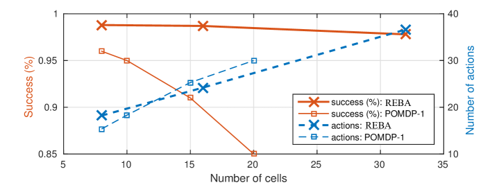
Figure 5: Ability to successfully achieve the assigned goal, and the number of actions executed before termination, as a function of the number of cells in the domain. REBA significantly increases accuracy and reduces the number of actions executed, in comparison with POMDP-1, as the number of cells in the domain increases.

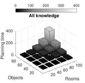
(a) Using all knowledge

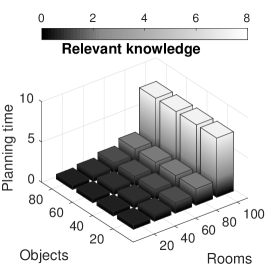
(b) Using relevant knowledge

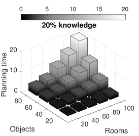
(c) Using some knowledge

Figure 6: Planning time as a function of the number of rooms and the number of objects in the domain—REBA only uses relevant knowledge for reasoning, and is thus able to scale to larger number of rooms and objects.

Next, we evaluated the time taken by REBA to generate a plan as the size of the domain increases. We characterize domain size based on the number of rooms and the number of objects in the domain. We conducted three sets of experiments in which the robot reasons with: (1) all available knowledge of domain objects and rooms; (2) only knowledge relevant to the assigned goal—e.g., if the robot knows an object’s default location, it need not reason about other objects and rooms in the domain to locate this object; and (3) relevant knowledge and knowledge of an additional $20\%$ of randomly selected domain objects and rooms. Figures 6(a)-6(c) summarize these results. We observe that using just the knowledge relevant to the goal to be accomplished significantly reduces the planning time. REBA supports the identification of such knowledge based on the refinement and zooming operations described in Section 7. As a result, robots equipped with REBA will be able to generate appropriate plans for domains with a large number of rooms and objects. Furthermore, if we only use a probabilistic approach (POMDP-1), it soon becomes computationally intractable to generate a plan for domains with many objects and rooms. These results are not shown in Figure 6, but they are documented in prior papers evaluating just the probabilistic component of the proposed architecture [62, 70].

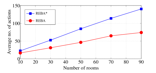
Figure 7: Effect of using default knowledge—principled representation of defaults significantly reduces the number of actions (and thus time) for achieving assigned goal.

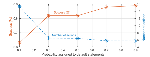
Figure 8: Ability to achieve goals, and number of actions executed, using only POMDPs, when different probability values are assigned to default statements and the ground truth locations of objects perfectly matches the default locations. The number of actions decreases and success (%) increases as the probability value increases.

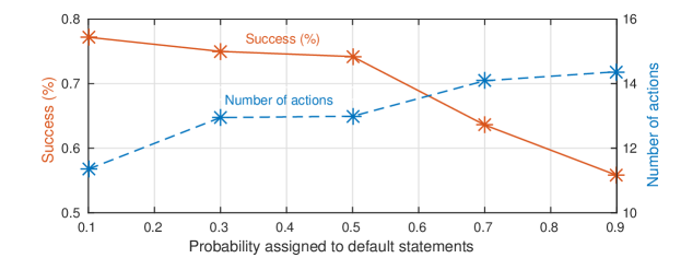
Figure 9: Ability to achieve goals, and number of actions executed, using only POMDPs, when different probability values are assigned to default statements and the ground truth locations of objects never matches the default locations. The number of actions increases and success (%) decreases as the probability value increases.

To evaluate hypothesis H3, i.e., to evaluate the effect of our representation and use of default knowledge on reliability and computational efficiency of decision making, we first conducted trials in which REBA was compared with $\mathcal{REBA}^{*}$, a version that does not include any default knowledge, e.g., when the robot is asked to fetch a textbook, there is no prior knowledge regarding the location of textbooks, and the robot explores the closest location first. Figure 7 summarizes the average number of actions executed per trial as a function of the number of rooms in the domain—each sample point in this figure is the average of $10000$ trials. The goal in each trial is (as before) to move a specific object to a specific place. We observe that our (proposed) representation and use of default knowledge significantly reduces the number of actions (and thus time) required to achieve the assigned goal.

Next REBA was compared with POMDP-2, a version of POMDP-1 that assigns specific probability values to default knowledge (e.g., “textbooks are in the library with probability $0.9$”) and suitably revises the initial belief state. The goal (once again) was to find and move objects to specific locations, and we measured the ability to successfully achieve the assigned goal and the number of actions executed before termination. Figures 8-9 summarize the corresponding results under two extreme cases representing a perfect match (mismatch) between the default locations and ground truth locations of objects. In Figure 8, the ground truth locations of target objects (unknown to the robot) match the default locations of the objects, i.e., there are no exceptions to the default statements. We observe that as the probability assigned to the default statement increases, the number of actions executed by the robot decreases and the fraction of trials completed successfully increases. However, for larger values along the x-axis, the difference in the robot’s performance for two different values of the probability (assigned to defaults) is not that significant. In Figure 8, the ground truth locations of the target objects never match the default locations of the objects, i.e., unknown to the robot, all trials correspond to exceptions to the default knowledge. In this case, the robot executes many more actions before termination and succeeds in a smaller fraction of trials as the probability value assigned to default statements increases. We also repeated these experimental trials after varying the extent to which the ground truth locations of objects matched their default locations. We noticed that when the probability assigned to default statements accurately reflects the ground truth, the number of trials in which the robot successfully achieves the goal increases and approaches the performance obtained with REBA. However, recall that computing the probabilities of default statements accurately takes a lot of time and effort. Also, these probabilities may change over time and the robot’s ability to achieve the assigned goals may be sensitive to these changes, making it difficult to predict the robot’s behavior with confidence. In addition, it is all the more challenging to accurately represent and efficiently use probabilistic information about prioritized defaults (e.g., Example 2). In general, we observed that the effect of assigning a probability value to defaults is arbitrary depending on factors such as (a) the numerical value chosen; and (b) the degree of match between ground truth and the default information. For instance, if a large probability is assigned to the default that books are typically in the library, but the book the robot has to move is an exception to the default (e.g., a cookbook), it takes significantly longer for POMDP-2 to recover from the initial belief. REBA, on the other hand, supports elegant representation of, and reasoning with, defaults and exceptions to these defaults.

Robot Experiments:

In addition to the trials in simulated domains, we implemented and evaluated REBA with POMDP-1 on physical robots using the Robot Operating System (ROS). We conducted experimental trials with two robot platforms (see Figure 1) in variants of the domain described in Example 1. Visual object recognition is based on learned object models that consist of appearance-based and contextual visual cues [42]. Since, in each trial, the robot’s initial location and the target object(s) are chosen randomly, it is difficult to compute a meaningful estimate of variance, and statistical significance is established through paired trials. In each paired trial, for each approach being compared (e.g., REBA or POMDP-1), the target object(s), the robot’s initial location, and the location of domain objects are the same, and the robot has the same initial domain knowledge.

First, we conducted $50$ trials on two floors of our Computer Science department building. This domain includes places in addition to those included in our illustrative example, e.g., Figure 1(a) shows a subset of the domain map of the third floor of the building, and Figure 1(b) shows the Peoplebot wheeled robot platform used in these trials. The robot is equipped with a stereo camera, laser range finder, microphone, speaker, and a laptop running Ubuntu Linux that performs all the processing. The domain maps are learned and revised by the robot using laser range finder data and the existing ROS implementation of a SLAM algorithm [15]. This robot has a manipulator arm that can be moved to reachable 3D locations relative to the robot. However, since robot manipulation is not a focus of this work, once the robot is next to the desired object, it extends its gripper and asks for the object to be placed in it. For experimental trials on the third floor, we considered $15$ rooms, which includes faculty offices, research labs, common areas and a corridor. To make it feasible to use POMDP-1 in such large domains, we used our prior work on a hierarchical decomposition of POMDPs for visual sensing and information processing that supports automatic belief propagation across the levels of the hierarchy and model generation in each level of the hierarchy [62, 70]. The experiments included paired trials, e.g., over $15$ trials (each), POMDP-1 takes $1.64$ as much time as REBA (on average) to move specific objects to specific places. For these paired trials, this $39\%$ reduction in execution time provided by REBA is statistically significant: p-value $=0.0023$ at the $95\%$ significance level.

Consider a trial in which the robot’s objective is to bring a specific textbook to the place named study_corner. The robot uses default knowledge to create a plan of abstract actions that causes the robot to move to and search for the textbook in the main_library. When the robot does not find this textbook in the main_library after searching using a suitable POMDP policy, replanning by the logician causes the robot to investigate the aux_library. The robot finds the desired textbook in the aux_library and moves it to the target location. A video of such an experimental trial can be viewed online at http://youtu.be/8zL4R8te6wg

To explore the applicability of REBA in different domains, we also conducted $40$ experimental trials using the Turtlebot wheeled robot platform in Figure 1(c) in a variant of the illustrative domain in Example 1. This domain had three rooms in the Electrical Engineering department building arranged to mimic a robot operating as a robot butler, with additional objects (e.g., tables, chairs, food items etc). The robot was equipped with a Kinect (RGB-D) sensor, a laser range finder, and a laptop running Ubuntu Linux that performs all the processing. As before, the robot used the ROS implementation of a SLAM algorithm, and a hierarchical decomposition of POMDPs for POMDP-1. This robot did not have a manipulator arm—once it reached a location next to the location of the desired object, it asks for the object to be placed on it. The experiments included paired trials, e.g., in $15$ paired trials, POMDP-1 takes $2.3$ as much time as REBA (on average) to move specific objects to specific places—this reduction in execution time by REBA is statistically significant at the $95\%$ significance level.

Consider a trial in which the robot’s goal was to fetch a bag of crisps for a human. The robot uses default knowledge about the location of the bag of crisps (e.g., that they are usually in the $kitchen$), to create a plan of abstract actions to achieve this goal. Execution of this plan causes the robot to first move to the $kitchen$ and search for the bag of crisps. The robot finds the bag of crisps, asks for the bag to be placed on it (since it has no manipulator), and moves back to $table1$ in $lab1$ (the location of the human who wanted the crisps), only to be told that it has brought a bag of chocolates instead. The robot diagnoses the cause for this unexpected observation as human error (i.e., that it was given incorrect bag in the $kitchen$ by a human). The robot then computes and executes a plan that has it go back and fetch the correct bag (of crisps) this time. A video of this trial can be viewed online at https://vimeo.com/136990534

11 Conclusions and Future Work

This paper described a refinement-based knowledge representation and reasoning architecture (REBA) that combines the complementary strengths of declarative programming and probabilistic graphical models. The architecture is based on tightly-coupled transition diagrams that represent domain knowledge, and the robot’s abilities and beliefs, at two levels of granularity. The architecture makes the following key contributions:

• Action language $\mathcal{AL}_{d}$ is extended to support non-Boolean fluents and non-deterministic causal laws, and is used to describe the coarse-resolution and fine-resolution transition diagrams.

• The notion of a history of a dynamic domain is extended to include default knowledge in the initial state, and a model of this history is defined. These definitions are used to define a notion of explanation of unexpected observations, and to provide an algorithm for coarse-resolution planning and diagnostics that translates history into a program of CR-Prolog, computes answer set of this program, and extracts plan and explanation (if needed) from the answer set.

• A formal definition is provided of one transition diagram being a weak refinement of another transition diagram, and a fine-resolution diagram is defined as a weak refinement of the domain’s coarse-resolution transition diagram.

• A theory of observations is introduced and a formal definition is provided of one transition diagram being a strong refinement of another transition diagram. This theory of observations is combined with the weakly refined fine-resolution transition diagram to obtain a fine-resolution transition diagram that is a strong refinement of the coarse-resolution transition diagram.

• The randomization of the fine-resolution transition diagram is defined, and an approach is described for experimental collection of statistics. These statistics are used to compute the probabilities of action outcomes and observations at the fine-resolution.

• A formal definition is provided for zooming to a part of the randomized fine-resolution diagram relevant to any given coarse-resolution (abstract) transition. This definition is used to automate the zoom operation and implement each abstract action in the coarse-resolution plan.

• An algorithm is provided for automatically constructing data structures appropriate for the fine-resolution probabilistic implementation of any given abstract action. This algorithm uses probabilistic models of the uncertainty in sensing and actuation, and the zoomed part of the fine-resolution transition diagram. The outcomes of the fine-resolution execution update the coarse-resolution history for subsequent reasoning.

• Finally, and possibly one of the major contributions, is a general methodology for the design of software components of robots that are re-taskable and robust. This design methodology is based on Dijkstra’s view of step-wise refinement of the specification of a program.

In this paper, the domain representation for coarse-resolution non-monotonic logical reasoning is translated to a CR-Prolog program, and the representation for probabilistic reasoning is translated to a POMDP. The key advantages of using this architecture are:

• It substantially simplifies the design process and increases confidence in the correctness of the robot’s behavior. In particular:

  • Step-wise refinement leads to clear separation of concerns and supports early testing of the different components of the architecture.

  • The formal (i.e., mathematical) descriptions of the different components, and of the flow of control and information between the components, helps characterize the robot’s behavior accurately and prove correctness of the algorithms.

  • The domain-independent representations of part of the commonsense knowledge used by the robot, e.g., theory of observations, weak refinement and strong refinement, allows for the reuse of these representations on other robots and application domains.

  • There is a single framework for inference, planning, diagnostics, and for a quantifiable trade off between accuracy and computational efficiency in the presence of probabilistic models of uncertainty in sensing and actuation.

• It significantly improves the computational efficiency and reliability of the robot’s actions. In particular:

  • The robot is able to reason reliably and efficiently with hierarchically-organized knowledge and beliefs.

  • Experimental results in simulation and on physical robots in different domains indicate the ability to reason at the sensorimotor level and the cognitive level with violation of defaults, noisy observations and unreliable actions.

  • The tight coupling between representation and reasoning at different resolutions, based on concepts such as refinement and zooming, supports precise reasoning while still demonstrating the potential to scale to complex domains.

The proposed architecture opens up many directions for further research, some of which relax the constraints imposed in the design of our current architecture. First, we will further explore the tight coupling between the transition diagrams, and between logical and probabilistic reasoning, in dynamic domains. We have, for instance, explored different resolutions for reasoning probabilistically [13], and investigated the inference, planning and diagnostics capabilities of architectures that reason at different resolutions [71]. However, we have so far not explored non-stationary domains, a limiting constraint that we seek to relax in future work. Second, our architecture has so far focused on a single robot, although we have instantiated the architecture in different domains. Another direction of further research is to extend the architecture to enable collaboration between a team of robots working towards a shared goal. It is theoretically possible to use our current architecture on multiple robots, but it will open up challenging questions and choices regarding communication (between robots) and propagation of beliefs held by different members of the team. Third, the proposed architecture has focused on representation and reasoning with incomplete knowledge, but a robot collaborating with humans in a dynamic domain also needs to be able to revise and augment its existing knowledge. Preliminary work in this direction, e.g., based on exploiting the complementary strengths of relational reinforcement learning, active (inductive) learning, and reasoning with commonsense knowledge, has provided promising results [59, 60, 61], and we seek to further explore this direction of work in the future. The long-term objective is to better understand the coupling between non-monotonic logical reasoning and probabilistic reasoning, and to use this understanding to develop architectures that enable robots to assist humans in complex domains.

Appendix A Proof of Proposition 1

In this section, we examine Proposition 1, which states that

If $\mathcal{D}$ is a well-founded system description and $\mathcal{H}$ is its recorded history, then every sequence induced by an answer set of $\Pi(\mathcal{D},\mathcal{H})$ is a model of $\mathcal{H}$.

To prove this proposition, we begin with some notation. Let $\sigma$ be a collection of literals, $\alpha_{k}=\langle a_{0},\dots,a_{k}\rangle$ be a (possibly empty) sequence of actions, $occurs(\alpha_{k})=\{occurs(a_{i},i):0\leq i\leq k\}$ and $\Pi(\mathcal{D},\sigma,\alpha_{k})=_{def}\Pi^{k+1}(\mathcal{D})\cup val(\sigma,0)\cup occurs(\alpha_{k})$.

Lemma 1.

Let $A$ be an answer set of $\Pi(\mathcal{D},\mathcal{H})$. Then there exists a state $\sigma_{0}$ of ${\tau(\mathcal{D})}$ and a sequence of actions $\alpha_{k}=\langle a_{0},\dots,a_{k}\rangle$ such that the set $B$ obtained from $A$ by removing literals formed by $obs$, $hpd$, $prefer$, $ab$ and $defined\_by\_default$ is an answer set of $\Pi(\mathcal{D},\sigma_{0},\alpha_{k})$.

Proof of Lemma 1.

Let $R$ be a set of CR-rules. By $\alpha(R)$ we denote the set of regular ASP rules obtained by replacing $\stackrel{{\scriptstyle\,\,+}}{{\leftarrow}}$ by $\leftarrow$ in rules of $R$. Let $\Pi$ be a program of CR-Prolog. By $\Pi^{reg}$ we denote the set of all regular rules of $\Pi$. A cardinality-minimal set of CR-rules of $\Pi$ such that ASP program $\Pi(R)=_{def}\Pi^{reg}\cup\alpha(R)$ is consistent, i.e. has an answer set, is called an abductive support of $\Pi$. $A$ is an answer set of $\Pi$ if it is an answer set of program $\Pi(R)$ for some abductive support $R$ of $\Pi$. Note that this is a special case of a more general definition from [23] where minimality of $R$ is determined by an arbitrary preference relation. Finally, recall that if $\sigma$ is a state of a transition diagram, $\sigma^{nd}$ is obtained from $\sigma$ by removing all atoms formed by defined fluents.

Now, let $A$ be an answer set of $\Pi=_{def}\Pi(\mathcal{D},\mathcal{H})$. Then, by the CR-Prolog definition of answer sets, we have:

1. $A$ is an answer set of an ASP program $\Pi(R)=\Pi^{reg}\cup\alpha(R)$ for some abductive support $R$ of $\Pi$.

Clearly, $\alpha(R)$ is (a possibly empty) collection of rules of the form: $ab(d(\bar{x}))\leftarrow val(body(d(\bar{x})),0)$. We will prove the existence of $\sigma_{0}$ and $\alpha_{k}$ by construction. Let:

1. $\sigma_{0}=\{f(\bar{x})=y:val(f(\bar{x}),y,0)\in A$ or $f(\bar{x})=y\in A\}$

We will show that $\sigma_{0}$ is a state of ${\tau(\mathcal{D})}$, i.e., that:

• $\sigma_{0}$ is an interpretation, i.e. for every $f(\bar{x})$ there is unique $y$ such that $f(\bar{x})=y\in\sigma_{0}$; and

• $\sigma_{0}$ is the unique answer set of program $\Pi_{c}(\mathcal{D})\cup\sigma_{0}^{nd}$.

To show (a) consider first an arbitrary basic fluent $f(\bar{x})$. Based on (2), for every $y$, $f(\bar{x})=y\in\sigma_{0}$ iff $val(f(\bar{x}),y,0)\in A$. Hence, we need to show that there is $y$ such that $val(f(\bar{x}),y,0)\in A$. There are two cases depending on whether or not the body of Statement 37 is satisfied by $A$. In the former case the existence of $y$ such that $val(f,y,0)\in A$ is guaranteed by Statement 30; otherwise it follows from Statement 38. If $f(\bar{x})$ is static, we have that there is $y$ such that $f(\bar{x})=y\in A$ by Statement 17 of $\Pi(\mathcal{D})$. If $f(\bar{x})$ is a defined fluent, its boolean value is included in $A$ by the axioms for the defined fluents (Statement 15). Uniqueness of the value assigned to $f(\bar{x})$ follows from Statement 20 and consistency of $A$.

To show (b) it suffices to notice that since $A$ satisfies rules such as Statement 14 in $\Pi(R)$, $\sigma_{0}$ satisfies rules such as Statement 8 in $\Pi_{c}(\mathcal{D})$, and hence $\Pi_{c}(\mathcal{D})\cup\sigma_{0}^{nd}$ has an answer set. By (a), $\sigma_{0}$ is complete and consistent and hence, by the definition of well-foundedness, this answer set is unique.

Next, let:

1. $\alpha_{k}=\langle a_{0},\dots,a_{k}\rangle$ where $a_{i}=\{e_{j}:occurs(e_{j},i)\in A\}$.

and let $S_{0}$ be a set of literals formed by $obs$ and $hpd$. Note that $S_{0}$ is a splitting set of program $\Pi(R)$. From (1) and the splitting set theorem [3] we have:

1. $A_{0}$, obtained from $A$ by removing literals formed by $obs$ and $hpd$, is an answer set of program $\Pi_{0}(R)$ obtained from $\Pi(R)$ by:

   • removing all atoms formed by $obs$ and $hpd$;

   • removing all rules whose bodies contain atoms formed of $obs(*,*,*)$ or $hpd(*,*)$ that are not in $A$; and

   • removing all occurrence of atoms $obs(*,*,*)$ or $hpd(*,*)$ from the remaining rules.

Note that the only rules changed by this transformation belong to the encoding of $\mathcal{H}$.

Next, if $\Pi_{0}^{\mathcal{H}}(R)$ denotes the program obtained from $\Pi_{0}(R)$ by removing all atoms formed by $occurs$ and all rules of $\Pi^{k+1}(\mathcal{D})$, then from (4) and the definition of $\Pi_{0}^{\mathcal{H}}(R)$ we have that:

1. $A_{0}$ is an answer set of $\Pi_{0}(R)=\Pi^{k+1}(\mathcal{D})\cup\Pi_{0}^{\mathcal{H}}(R)\cup\{occurs(a,i):occurs(a,i)\in A\}$.

Now let $S_{1}$ be the set of atoms formed by statics, $prefer$, $ab$, $defined\_by\_default$, and $val(*,*,0)$. It is not difficult to check that $S_{1}$ is a splitting set of $\Pi_{0}(R)$. It divides the program into two parts:

• Program $Bot$ consisting of $\Pi_{0}^{\mathcal{H}}(R)$ combined with the set $Zero$ of instances of axioms encoded in Statements 14, 15,  17 and 20 from $\Pi^{k+1}(\mathcal{D})$ with the time-step variable set to $0$.

• Program $Top=(\Pi^{k+1}(\mathcal{D})\setminus Zero)\cup\{occurs(a,i):occurs(a,i)\in A\}$

So, by the splitting set theorem, we now have:

1. $A_{0}$ is an answer set of program $B_{0}\cup Top$ where $B_{0}$ is an answer set of $Bot$.

Next, observe that:

1. $B_{0}$ can be partitioned into $B_{1}$ and $B_{2}$ with $B_{1}$ consisting of atoms of $A_{0}$ formed by $prefer$, $ab$, and $defined\_by\_default$ and $B_{2}$ consisting of atoms of $A_{0}$ formed by statics and $val(*,*,0)$.

Using definition of answer sets for ASP program, it can be proved that for any two programs $\Pi_{1}$ and $\Pi_{2}$ whose signatures $\Sigma_{1}$ and $\Sigma_{2}$ are disjoint, $X$ is an answer set of a program $\Pi_{1}\cup\Pi_{2}$ iff $X|_{\Sigma_{1}}$ and $X|_{\Sigma_{2}}$ are answer sets of $\Pi_{1}$ and $\Pi_{2}$ respectively. Hence, we have that:

1. $B=A_{0}\setminus B_{1}$ is an answer set of $B_{2}\cup Top$.

From (4), (7) and (8) above, we have that $B$ is obtained from $A$ by removing literals formed by $obs$, $hpd$, $prefer$, $ab$ and $defined\_by\_default$.

To show that $B$ is an answer set of $\Pi(\mathcal{D},\sigma_{0},\alpha_{k})$ we first demonstrate that:

1. $B$ is an answer set of $\Pi_{1}^{*}=_{def}B_{2}\cup\Pi^{k+1}(\mathcal{D})\cup\{occurs(a,i):occurs(a,i)\in A\}$.

By construction, we have that:

1. $\Pi_{1}^{*}=B_{2}\cup Top\cup Zero$.

To prove (9), we will show that $B$ is an answer set of the reduct, $(\Pi_{1}^{*})^{B}$ of $\Pi_{1}^{*}$ with respect to $B$ (note that this is the definition of answer set). Based on the definition of the reduct and (10), we have:

1. $(\Pi_{1}^{*})^{B}=B_{2}\cup Zero^{B}\cup Top^{B}$.

From (8) and the definition of answer set, we have that $B$ is a $\subseteq$-minimal set satisfying $B_{2}\cup Top^{B}$. Then, based on (6)-(8), we have that $B_{2}$ (and hence $B$) also satisfies $Zero^{B}$, and thus (9) holds.

Then, based on (2), (6) and (7), we have that $val(\sigma_{0},0)=B_{2}$ which, together with (9), implies that:

1. $B$ is an answer set of $\Pi^{k+1}(\mathcal{D},\sigma_{0},\alpha_{k})$.

This completes the proof of Lemma 1. ∎

Lemma 2.

Let $B$ be an answer set of $\Pi(\mathcal{D},\sigma_{0},\alpha_{k})$, $B_{k}$ be obtained from $B$ by removing all literals containing time-step $k+1$, and $\Pi_{k}^{k+1}(\mathcal{D},\sigma_{k},a_{k})$ be $\Pi(\mathcal{D},\sigma_{k},a_{k})$ with time-steps $0$ and $1$ replaced by $k$ and $k+1$ respectively. Then:

• $B_{k}$ is an answer set of $\Pi(\mathcal{D},\sigma_{0},\alpha_{k-1})$.

• $B=B_{k}\cup U$ where $U$ is an answer set of $\Pi_{k}^{k+1}(\mathcal{D},\sigma_{k},a_{k})$.

Proof of Lemma 2.

Let $S$ be a set of literals of $\Pi(\mathcal{D},\sigma_{0},\alpha_{k})$ not containing time step $k+1$. It is easy to check that $S$ is a splitting set of this program, which divides it into two parts:

1. $Bot=\Pi(\mathcal{D},\sigma_{0},\alpha_{k-1})$ and $Top=\Pi(\mathcal{D},\sigma_{0},\alpha_{k})\setminus Bot$.

By the splitting set theorem and definition of $B_{k}$, we have:

1. $B_{k}$ is an answer set of $Bot=\Pi(\mathcal{D},\sigma_{0},\alpha_{k-1})$.

and:

1. $B$ is an answer set of the program $B_{k}\cup Top$.

By definition, $\sigma_{k}=\{f(\bar{x})=y:val(f(\bar{x}),y,k)\in B\}\cup\{f(\bar{x})=y:f(\bar{x})=y\in B\}$, and hence, $val(\sigma_{k},k)$ is a subset of $B$ and of $B_{k}$. Thus, we have:

1. $B_{k}\cup Top=B_{k}\cup val(\sigma,k)\cup Top=B_{k}\cup\Pi_{k}^{k+1}(\mathcal{D},\sigma_{k},a_{k})$.

Now let:

1. $B_{k}=B_{k}^{\prime}\cup B_{k}^{\prime\prime}$

where $B_{k}^{\prime}$ consists of atoms of $B_{k}$ containing time-steps smaller than $k$ and $B_{k}^{\prime\prime}=B_{k}\setminus B_{k}^{\prime}$. Note that $B_{k}^{\prime\prime}$ consists of atoms of $B_{k}$ formed by statics and of those containing time-step $k$. From (4), (5), and the definition of $\sigma_{k}$, we then have:

1. $B_{k}\cup Top=B_{k}^{\prime}\cup\Pi_{k}^{k+1}(\mathcal{D},\sigma_{k},a_{k})$.

Based on (3) and (6), we have:

1. $B$ is an answer set of $B_{k}^{\prime}\cup\Pi_{k}^{k+1}(\mathcal{D},\sigma_{k},a_{k})$.

Since, by construction, the signatures of $B_{k}^{\prime}$ and $\Pi_{k}^{k+1}(\mathcal{D},\sigma_{k},a_{k})$ are disjoint, from (7), we have:

1. $B=B_{k}\cup U$ where $U$ is an answer set of $\Pi_{k}^{k+1}(\mathcal{D},\sigma_{k},a_{k})$.

This completes the proof of Lemma 2. ∎

Proof of Proposition 1.

Let $\mathcal{D}$ and $\mathcal{H}$ be as in the proposition, $A$ be an answer set of CR-Prolog program $\Pi(\mathcal{D},\mathcal{H})$, and $M=\langle\sigma_{0},a_{0},\sigma_{1},\dots,\sigma_{n},a_{n},\sigma_{n+1}\rangle$ be a sequence induced by $A$. We will show that $M$ is a model of $\mathcal{H}$, i.e. $M$ is a path of transition diagram ${\tau(\mathcal{D})}$ (definition 6).

The proposition will be an immediate consequence of a more general statement:

1. for every $0\leq k\leq n+1$ $M_{k}=\langle\sigma_{0},a_{0},\sigma_{1},\dots,\sigma_{k}\rangle$ is a path in ${\tau(\mathcal{D})}$.

Before proceeding with inductive proof of (1), let us notice that, by Lemma 1:

1. $M$ is induced by an answer set $B$ of an ASP program $\Pi(\mathcal{D},\sigma_{0},\alpha_{n})$ where $\sigma_{0}$ is a state and $B$ is obtained from $A$ by removing atoms formed by $obs$, $hpd$, $prefer$, $ab$ and $defined\_by\_default$.

We use induction on $k$. The base case is: $k=0$, i.e. $M_{k}=\langle\sigma_{0}\rangle$. Then (1) follows immediately from (2).

Nex, consider the inductive step: let $k>0$ and $M_{k}=\langle\sigma_{0},a_{0},\sigma_{1},\dots,\sigma_{k-1},a_{k-1},\sigma_{k}\rangle$. By inductive hypothesis:

1. $M_{k}=\langle\sigma_{0},a_{0},\sigma_{1},\dots,\sigma_{k-1}\rangle$ is a path in ${\tau(\mathcal{D})}$.

We need to show that $L=\langle\sigma_{k-1},a_{k-1},\sigma_{k}\rangle$ is a transition of ${\tau(\mathcal{D})}$. By Lemma 2, we have:

1. $L$ is induced by an answer set $U_{0}$ of $\Pi_{k}^{k+1}(\mathcal{D},\sigma_{k},a_{k})$.

Let $U$ be obtained from $U_{0}$ by replacing time-steps $k$ and $k+1$ by $0$ and $1$ respectively. From (4) and the definition of $\Pi_{k}^{k+1}(\mathcal{D},\sigma_{k},a_{k})$, we have that:

1. $L$ is induced by an answer set $U$ of $\Pi(\mathcal{D},\sigma_{k},a_{k})$.

From (3) we have that:

1. $\sigma_{k}$ is a state.

To prove that $\sigma_{k+1}$ is a state we first show that $\sigma_{k+1}$ is an interpretation, i.e. for every $f(\bar{x})$ there is unique $y$ such that $val(f(\bar{x}),y,1)\in U$. From (5) and (6), we have that, for every $f(\bar{x})$ there is unique $y_{1}$ such that $val(f(\bar{x}),y,0)\in U$. If the body of the inertia axiom for $f(\bar{x})$ is satisfied by $U$ then $val(f(\bar{x}),y_{1},1)\in U$. Otherwise, the inertia axiom is defeated by Statement 20 and hence $val(f(\bar{x}),y_{2},1)\in U$. Thus, we have that:

1. $\sigma_{k+1}$ is an interpretation.

The last step is to show that:

1. $\sigma_{k+1}$ is the unique answer set of program $\Pi_{c}(\mathcal{D})\cup\sigma_{k+1}^{nd}$.

To do that it suffices to notice that, since $U$ satisfies rules such as Statements 15 and 14 in $\Pi(\mathcal{D},\sigma_{k},a_{k})$, $\sigma_{k+1}$ satisfies rules such as Statements 8 and 9 in $\Pi_{c}(\mathcal{D})$, and hence $\Pi_{c}(\mathcal{D})\cup\sigma_{k+1}^{nd}$ has an answer set. Based on (7), $\sigma_{k+1}$ is complete and consistent and hence, by the definition of well-foundedness, this answer set is unique; this proves (8). Then, based on (7) and (8), and the definition of state, we have:

1. $\sigma_{k+1}$ is a state.

Thus, based on (5),  (6),  (9) and Definition 4, we have that:

1. $L$ is a transition.

Next, based on (3), the definition of $L$, and (10):

1. $M_{k}$ is a path in ${\tau(\mathcal{D})}$.

This completes the proof of statement (1). Based on the definition of $M_{k}$, $M=M_{n+1}$, and based on (1), $M$ is a path in ${\tau(\mathcal{D})}$. Since $M$ is induced by $A$, based on Definition 6, it is a model of $\mathcal{H}$. This completes the proof of Proposition 1. ∎

Appendix B Proof of Proposition 2

In this section, we examine Proposition 2, which states that:

Let $\mathcal{P}=(\mathcal{D},\mathcal{H},h,G)$ be a planning problem with a well-founded, deterministic system description $\mathcal{D}$. A sequence $\langle a_{0},\dots,a_{k-1}\rangle$ where $k<h$ is a solution of $\mathcal{P}$ iff there is an answer set $A$ of $Plan$ such that:

1. For any $n<i\leq n+k$, $occurs(a_{i},i-1)\in A$,

2. $A$ contains no other atoms of the form $occur(*,i)$ with $i\geq n$.

We begin by introducing some notation. Let $\Pi$ be an arbitrary CR-Prolog program and $R$ be a collection of CR-rules from $\Pi$. Similar to the terminology in [23], we use $\Pi^{reg}$ to denote the collection of regular rules of $\Pi$ and $\alpha(R)$ to denote the set of regular ASP rules obtained by replacing $\stackrel{{\scriptstyle\,\,+}}{{\leftarrow}}$ by $\leftarrow$ in CR-rules of $R$. For completeness, recall that for any program $\Pi$, we have $\Pi(R)=\Pi^{reg}\cup\alpha(R)$. Also recall, from Section 5.3, that:

$$Plan=Diag~{}\cup~{}Classical\_plan~{}\cup~{}\{DPC\}$$

$$Diag=_{def}\Pi^{n}(\mathcal{D},\mathcal{H})$$

$$Classical\_plan=\Pi^{[n..n+h]}(\mathcal{D})~{}\cup~{}goal(I)\leftarrow val(f(\bar{x}),y,I)~{}\cup~{}PM$$

$$\leftarrow Y=count\{X:ab(X)\},Y>m~{}~{}~{}~{}~{}~{}~{}~{}~{}\textrm{\% DPC}$$

where $n$ is the current step of $\mathcal{H}$, $m$ is the size of the abductive support of $Diag$, and $PM$ is the planning module. We will also need the following Lemma to prove Proposition 2.

Lemma 3.

For any set $R$ of CR-rules of $Diag$, $A$ is an answer set of ASP program $Plan(R)$ iff $A=A_{0}\cup B_{0}$ where $A_{0}$ is an answer set of $Diag(R)$ satisfying $DPC$ and $B_{0}$ is an answer set of $Shifted\_plan=_{def}\{val(f(\bar{x}),y,n):val(f(\bar{x}),y,n)\in A_{0}\}\cup Classical\_plan$.

Proof of Lemma 3.

Let $S_{0}$ be the set of literals of $Plan(R)$ not containing atoms with time steps greater than $n$ or atoms of the form $occurs(*,n)$ and $hpd(*,n)$. It is easy to check that $S_{0}$ is a splitting set of $Plan(R)$ which splits the program into two parts, $Bot=Diag(R)\cup\{DPC\}$ and $Top=Classical\_plan$. By the splitting set theorem, $A$ is an answer set of $Plan(R)$ iff $A$ is an answer set of $A_{0}\cup Top$ where $A_{0}$ is an answer set of $Bot$. Clearly, $A_{0}\cup Top=A_{0}\cup Shifted\_plan$. Since $A_{0}$ is a collection of atoms, from the definition of answer set we have that $A=A_{0}\cup B_{0}$ where $B_{0}$ is an answer set of $Shifted\_plan$. ∎

Next, we turn to proving Proposition 2.

Proof of Proposition 2.

Let $\mathcal{P}$ and $Plan$ be as in the proposition, $\sigma$ be a state and $\langle a_{0},\dots,a_{k-1}\rangle$ with $k<h$ be a sequence of actions of $\mathcal{D}$.

Based on Definition 8:

1. $\langle a_{0},\dots,a_{k-1}\rangle$ is a solution of $\mathcal{P}$ iff:

   • there is a state $\sigma$ that is the current state of some model $M$ of $\mathcal{H}$; and

   • $\langle a_{0},\dots,a_{k-1}\rangle$ is a solution of classical planning problem $\mathcal{P}_{c}=(\mathcal{D},\sigma,G)$ with horizon $h$.

Based on Definition 6 and the well-foundedness of $\mathcal{D}$, Statement (a)(a) holds iff:

1. $M$ is induced by some answer set $A_{0}$ of $Diag$, $n$ is the current step of history from $\mathcal{P}$, and:

   $$\sigma=\{f(\bar{x})=y:val(f(\bar{x}),y,n)\in A_{0}\}$$

By the CR-Prolog definition of answer sets, Statement (2) holds iff:

1. $A_{0}$ is an answer set of $Diag(R)$ for some abductive support $R$ of $Diag$ and $\sigma=\{f(\bar{x})=y:val(f(\bar{x}),y,n)\in A_{0}\}$ (since $A_{0}$ is an answer set of $Diag$ it satisfies $DPC$).

Based on Proposition $9.1.1$ from [23], Statement (1)(b) holds iff:

1. There is an answer set $S$ of ASP program $plan(\mathcal{P}_{c},h)$ such that:

   • For any $0<i\leq k$, $occurs(a_{i},i-1)\in S$; and

   • $S$ contains no other atoms formed by $occurs$.

Consider an ASP program:

$$Shifted\_plan=_{def}\{val(f(\bar{x}),y,n):val(f(\bar{x}),y,n)\in A_{0}\}~{}\cup~{}Classical\_plan$$

It is easy to see that this program differs from $plan(\mathcal{P}_{c},h)$ only in the domain of its time-step variables. In the former case, such variables range over $[n,n+h]$ while in the latter the range is $[0,h]$. The programs are isomorphic and hence Statement (4) holds for $S$ iff:

1. $B_{0}$ obtained from $S$ by increasing all occurrences of time steps in atoms from $S$ by $n+1$ is an answer set of $Shifted\_plan$. Also:

   • For any $n<i\leq n+k$, $occurs(a_{i},i-1)\in B_{0}$; and

   • $B_{0}$ contains no other atoms of the form $occurs(*,i)$ where $i\geq n$.

Now we have that:

1. Statement (1) is true iff Statement (3) and Statement (5) are true.

Let $A=A_{0}\cup B_{0}$. Then, based on Lemma 3, we have:

1. Statements (3) and (5) are true iff $A$ is an answer set of $Plan(R)$.

Based on (7), we have:

1. Statement (1) is true iff $A$ is an answer set of $Plan(R)$.

However, since every answer set of $Plan$ must satisfy $DPC$, $Plan(R)$ has an answer set iff $R$ is an abductive support of $Plan$. Hence:

1. $A$ is an answer set of $Plan(R)$ iff $A$ is an answer set of $Plan$.

From the construction of $A$, Statement (5), and the fact that $A_{0}$ contains no atoms of the form $occurs(*,i)$ where $i\geq n$, we have that $A$ satisfies the conditions of the proposition. This completes the proof of Proposition 2. ∎

Appendix C Proof of Proposition 3

In this section, we prove Proposition 3, which states that:

Let $\mathcal{D}_{H}$ and $\mathcal{D}_{L,nobs}$ be coarse and fine resolution system descriptions from our running example. Then $\tau_{L}$ is a weak refinement of $\tau_{H}$.

Proof of Proposition 3.

Definitions in $\mathcal{D}_{H}$ and $\mathcal{D}_{L,nobs}$ contain no dependency between defined domain functions and their negations. Both system descriptions are therefore weakly-acyclic and thus well-founded, which justifies the use of the following property in the proof. Let $\mathcal{D}$ over signature $\Sigma$ be a well-founded system description defining transition diagram $\tau$. Then, an interpretation $\delta$ of $\Sigma$ is a state of $\tau_{H}$ iff:

• $\delta$ satisfies constraints of $\mathcal{D}$; and

• For every defined fluent $f$ of $\Sigma$, $f(\bar{u})\in\delta$ iff there is a rule from the definition of $f(\bar{u})$ whose body is satisfied by the interpretation $\delta$.

For readability, we also repeat Definition 9 of weak refinement of a transition diagram. A transition diagram $\tau_{L,nobs}$ over $\Sigma_{L,nobs}$ is called a weak refinement of $\tau_{H}$ if:

1. For every state $\sigma^{\diamond}$ of $\tau_{L,nobs}$, the collection $\sigma^{\diamond}|_{\Sigma_{H}}$ of atoms of $\sigma^{\diamond}$ formed by symbols from $\Sigma_{H}$ is a state of $\tau_{H}$.

2. For every state $\sigma$ of $\tau_{H}$, there is a state $\sigma^{\diamond}$ of $\tau_{L,nobs}$ such that $\sigma^{\diamond}$ is an extension of $\sigma$.

3. For every transition $T=\langle\sigma_{1},a^{H},\sigma_{2}\rangle$ of $\tau_{H}$, if $\sigma^{\diamond}_{1}$ and $\sigma^{\diamond}_{2}$ are extensions of $\sigma_{1}$ and $\sigma_{2}$ respectively, then there is a path $P$ in $\tau_{L,nobs}$ from $\sigma^{\diamond}_{1}$ to $\sigma^{\diamond}_{2}$ such that:

   • actions of $P$ are concrete, i.e., directly executable by robots; and

   • $P$ is pertinent to $T$, i.e., all states of $P$ are extensions of $\sigma_{1}$ or $\sigma_{2}$.

To prove the first clause of Definition 9, let $\sigma^{\diamond}$ and $\sigma=\sigma^{\diamond}|_{\Sigma_{H}}$ be as in the first clause. To prove that $\sigma$ is a state of $\mathcal{D}_{H}$, we show that it satisfies the clauses of the property described above. We start with the constraint in Statement 42(a) for a particular object $ob$:

$$loc(ob)=P~{}~{}\mathbf{if}~{}~{}loc(rob_{1})=P,~{}in\_hand(rob_{1},ob)$$

Let:

1. $(loc(rob_{1})=P)\in\sigma$; and

2. $in\_hand(rob_{1},ob)\in\sigma$.

To show that $(loc(ob)=P)\in\sigma$ let $c_{1}$ be the value of $loc^{*}(rob_{1})$ in $\sigma^{diamond}$, i.e:

1. $(loc^{*}(rob_{1})=c_{1})\in\sigma^{\diamond}$

Based on the bridge axiom in Statement 48(a):

$$loc(rob_{1})=P~{}~{}\mathbf{if}~{}~{}loc^{*}(rob_{1})=C,component(C,P)$$

of $\mathcal{D}_{L,nobs}$ and conditions $(i)$ and $(iii)$, we have:

1. $component(c_{1},P)$

Suppose this is not the case. Then, based on the definition of $place^{*}$, there is some place $P_{2}$ such that $component(c_{1},P_{2})\in\sigma^{\diamond}$. This statement, together with $(iii)$ and the bridge axiom in Statement 48(a) will entail $(loc(rob)=P_{2})$, which contradicts condition $(i)$ above.

Next, the state constraint in Statement 45(a):

$$loc^{*}(ob)=P~{}~{}\mathbf{if}~{}~{}loc^{*}(rob_{1})=P,~{}in\_hand(rob_{1},ob)$$

of $\mathcal{D}_{L,nobs}$, together with $(ii)$ and $(iii)$ imply:

1. $(loc^{*}(ob)=c_{1})\in\sigma^{\diamond}$

Then, the bridge axiom in Statement 48(a), together with $(iv)$ and $(v)$ imply that $(loc(ob)=P)\in\sigma$ and hence $\sigma$ satisfies the first constraint of $\mathcal{D}_{H}$.

Next, consider the definition of the static $next\_to(P_{1},P_{2})$ in $\mathcal{D}_{H}$. It our example domain with four rooms (see Figure 3(b)), $\mathcal{D}_{H}$ consists of statements such as:

$$next\_to(r_{1},r_{2})$$

$$next\_to(r_{1},r_{3})$$

$$next\_to(r_{2},r_{4})$$

$$next\_to(r_{3},r_{4})\$$

and the constraint:

$$next\_to(P_{1},P_{2})~{}~{}\mathbf{if}~{}~{}next\_to(P_{2},P_{1})$$

In the fine-resolution system description $\mathcal{D}_{L,nobs}$, these statements are replaced by a collection of statements of the form $next\_to^{*}(c_{i},c_{j})$, state constraint in Statement 45(b):

$$next\_to^{*}(C_{1},C_{2})~{}~{}\mathbf{if}~{}~{}next\_to^{*}(C_{2},C_{1})$$

and a bridge axiom as described by Statement 48(b):

$$next\_to(P_{1},P_{2})~{}~{}\mathbf{if}~{}~{}next\_to^{*}(C_{1},C_{2}),component(C_{1},P_{1}),component(C_{1},P_{2})$$

The last axiom implies that $next\_to(r_{i},r_{j})\in\sigma$ iff $\sigma^{\diamond}$ indicates that there are two adjacent cells in the domain such that one of them is in $r_{i}$ and another is in $r_{j}$. This is the situation in our example domain, as shown in Figure 3(b). This concludes the proof of the first clause of Definition 9.

To prove clause 2 of Definition 9, consider a state $\sigma$ of $\tau_{H}$ and expand it to a state $\sigma^{\diamond}$ of $\tau_{L,nobs}$, and show that $\sigma^{\diamond}$ is a state of $\tau_{L,obs}$. We do so by construction by interpreting the fine-resolution domain functions of $\mathcal{D}_{L,nobs}$ such that it satisfies the bridge axioms, constraints and definitions of $\mathcal{D}_{L,nobs}$. In our example domain, it is sufficient to map $loc^{*}(thing)$ to a cell $c$ of room $r$ such that:

• if $loc^{*}(th)=c$ and $component(c,rm)$ are in $\sigma^{\diamond}$ then $loc(th)=rm\in\sigma$

• if $in\_hand(rob_{1},ob)\in\sigma$ then the same cell is assigned to $rob_{1}$ and $ob$.

The definition of static $next\_to^{*}$ is the same for every state. It is symmetric and satisfies Statement 48(b) describing the bridge axiom for $next\_to$. In other words, all state constraints and definitions of $\mathcal{D}_{L,nobs}$ are satisfied by $\sigma^{\diamond}$, which is thus a state of $\tau_{L,nobs}$.

To prove the last clause of Definition 9, consider a transition $T=\langle\sigma_{1},move(rob,r_{2}),\sigma_{2}\rangle$ of $\tau_{H}$ and let $\sigma^{\diamond}_{1}$ and $\sigma^{\diamond}_{2}$ be states of $\tau_{L,nobs}$ expanding $\sigma_{1}$ and $\sigma_{2}$ respectively. Assume that the robot is in cell $c_{1}$ of room $r_{1}$ and that the robot’s desired position in $\sigma^{\diamond}_{2}$ is $c_{2}$. The required path $P$ then will consist of a sequence of moves of the form $move^{*}(rob_{1},c_{i})$ which starts with robot being at $c_{1}$ and ends with it being at $c_{2}$. Due to executability condition encoded in Statement 43(b) for $move(rob_{1},r_{2})$ rooms $r_{1}$ and $r_{i}$ are next to each other. Since our definition of $next\_to^{*}$ is such that the robot can always move to a neighboring cell and every two cells in rooms $r_{1}$ and $r_{2}$ are connected by paths which do not leave these rooms, clause 3 of Definition 9 is satisfied. Thus, $\tau_{L,nobs}$ in our running example is a weak refinement of $\tau_{H}$. ∎

Appendix D Proof of Proposition 4

In this section, we prove Proposition 4, which states that:

Let $\mathcal{D}_{H}$ and $\mathcal{D}_{L}$ be coarse and fine resolution system descriptions from our running example. Then $\tau_{L}$ is a strong refinement of $\tau_{H}$.

Proof of Proposition 4.

For readability, we repeat the Definition 10 of a strong refinement of a transition diagram. A transition diagram $\tau_{L}$ over $\Sigma_{L}$ is called a strong refinement of $\tau_{H}$ if:

1. For every state $\sigma^{\diamond}$ of $\tau_{L}$, the collection $\sigma^{\diamond}|_{\Sigma_{H}}$ of atoms of $\sigma^{\diamond}$ formed by symbols from $\Sigma_{H}$ is a state of $\tau_{H}$.

2. For every state $\sigma$ of $\tau_{H}$, there is a state $\sigma^{\diamond}$ of $\tau_{L}$ such that $\sigma^{\diamond}$ is an extension of $\sigma$.

3. For every transition $T=\langle\sigma_{1},a^{H},\sigma_{2}\rangle$ of $\tau_{H}$, if $\sigma^{\diamond}_{1}$ is an extension of $\sigma_{1}$, then for every observable fluent $f$ such that $observable_{f}(rob_{1},\bar{x},y)\in\sigma_{2}$, there is a path $P$ in $\tau_{L}$ from $\sigma^{\diamond}_{1}$ to an extension $\sigma^{\diamond}_{2}$ of $\sigma_{2}$ such that:

   • $P$ is pertinent to $T$, i.e., all states of $P$ are extensions of $\sigma_{1}$ or $\sigma_{2}$;

   • actions of $P$ are concrete, i.e., directly executable by robots; and

   • $observed_{f}(rob_{1},x,y)=true\in\sigma^{\diamond}_{2}$ iff $(f(x)=y)\in\sigma^{\diamond}_{2}$, and $observed_{f}(rob_{1},x,y)=false\in\sigma^{\diamond}_{2}$ iff $(f(x)=y_{1})\in\sigma^{\diamond}_{2}$ and $y_{1}\not=y$.

The first two clauses of Definition 10 follow immediately from the following observations:

• The states of $\tau_{L,nobs}$ and $\tau_{L}$ differ only by the knowledge functions. This follows immediately from the definition of a state and an application of the splitting set theorem.

• Both conditions are satisfied by the states of $\tau_{L,nobs}$; this follows from Proposition 3.

To prove the third clause of Definition 10, consider a transition $T=\langle\sigma_{1},a^{H},\sigma_{2}\rangle\in\tau_{H}$. There are two fluents $loc$ and $in\_hand$ that are observable in $\tau_{H}$. We start with the case in which the observable fluent is of the form:

$$loc(th)=rm$$

Based on the third condition of the third clause of the proposition:

1. $observable_{loc}(rob_{1},th,rm)\in\sigma_{2}$

Based on the definition of $observable_{loc}$ for our example, this can happen only if:

1. $loc(rob_{1})=rm\in\sigma_{2}$

Let $\delta^{\diamond}_{0}$ be a state of $\tau_{L}$ containing $\sigma_{2}$. Then:

1. $loc(rob_{1})=rm\in\delta^{\diamond}_{0}$

The value of $loc(th)$ in $\delta^{\diamond}_{0}$ is determined by the bridge axiom in Statement 48(a) and hence Statement (3) holds iff for some cell $c_{1}$ of $rm$:

1. $loc^{*}(rob_{1})=c_{1}\in\delta^{\diamond}_{0}$

Since by the definition of strong refinement, $\tau_{L}$ is also a weak refinement of $\tau_{H}$, Proposition 3 implies that there is a path $P_{1}$ of concrete action pertinent to $T$ from extension $\sigma^{\diamond}_{1}$ of $\sigma_{1}$ to $\delta^{\diamond}_{0}$.

There can be two possible cases:

$$(i)~{}~{}loc(th)=rm\in\sigma_{2}$$

$$(ii)~{}~{}loc(th)=rm\not\in\sigma_{2}$$

In case (i), an argument similar to the one described above shows that there is a state $\delta^{\diamond}_{1}$ of $\tau_{L}$ containing $\sigma_{2}$ such that for some cell $c_{2}$ of room $rm$:

1. $loc^{*}(th)=c_{2}\in\delta^{\diamond}_{1}$

Now, let $P_{2}$ be the shortest sequence of the robot’s moves from cell $c_{1}$ to cell $c_{2}$. Let $\delta^{\diamond}_{2}$ be the last state of this path. If at $\delta^{\diamond}_{0}$ the robot was already holding the thing $th$, then $P_{2}$ is empty. If the robot is not holding $th$, the moves of the robot do not change the location of $th$. Hence, we have:

1. $loc^{*}(thing)=c_{2}\in\delta^{\diamond}_{2}$

2. $loc^{*}(rob)=c_{2}\in\delta^{\diamond}_{2}$

Statements (6) and (7), together with the definition of $can\_be\_observed_{loc^{*}}$ imply that:

1. $can\_be\_observed_{loc^{*}}(rob,thing,c_{2})\in\delta^{\diamond}_{2}$

The robot can now execute the knowledge-producing action $test_{loc^{*}}(rob_{1},th,c_{2})$, which moves the system into the state $\sigma^{\diamond}_{2}$. Since this action does not change the values of physical fluents, locations of the robot and the thing remain unchanged. Now $observed_{loc}(rob_{1},th,rm)\in\sigma^{\diamond}_{2}$ follows from Statements 50 and 54(a). Notice that actions in the path $P$ defined as the concatenation of $P_{1}$, $P_{2}$ and $\langle\delta^{\diamond}_{2},test_{loc^{*}}(rob_{1},th,c_{2}),\sigma^{\diamond}_{2}\rangle$ are concrete and relevant to $T$, and satisfies the conditions of the third clause of Definition 10.

In case (ii), i.e., with $loc(th)=rm\not\in\sigma_{2}$, let $P_{1}$ be as before (i.e., a path of concrete action relevant to $T$ from $\sigma^{\diamond}_{1}$ to $\delta^{\diamond}_{0}$), $c_{1},\ldots,c_{n},c_{1}$ be a sequence visiting all the cells of $rm$, and $P$ be the concatenation of $P_{1}$ and the path $P_{2}$ of the form $\langle\delta^{\diamond}_{i},move(rob_{1},c_{i+1}),test_{loc^{*}}(rob_{1},th,c_{i+1}),\delta^{\diamond}_{i+1}\rangle$.

Since every thing is assumed to have a location, $th$ is in some room, say $rm_{1}$ different from $rm$. Since $loc(th)$ in determined by the bridge axiom in Statement 48(a) and no grid cell can belong to two different rooms, there is some cell $c$ different from $c_{1},\ldots,c_{n}$ such that $loc(th)=c$. Note that initially $observed_{loc}(rob_{1},th,rm)$ and $observed_{loc^{*}}(rob_{1},th,c)$ are $undet$ for every $c$ in $rm$. Since the thing $th$ is not in any cell of $rm$, $test_{loc^{*}}(rob_{1},th,c)$ will return false for every $c\in rm$. This means that Statement 54(b) is not applicable, and Statement 54(c) implies that $may\_be\_true_{loc}(rob,thing,rm)$ holds only until the robot reaches location $c_{1}$ and performs $test_{loc^{*}}(rob_{1},th,c_{1})$. In the resulting state, $\sigma^{\diamond}_{2}$, there is no component $c$ of $rm$ in which $observed_{loc^{*}}(rob_{1},th,c)$ is $undet$. The value of the defined fluent $may\_be\_true_{loc}(rob,thing,rm)$ is therefore false in $\sigma^{\diamond}_{2}$. Based on Statement 54(d), we conclude that $\sigma^{\diamond}_{2}$ contains $observed_{loc}(rob_{1},th,rm)=false$. Hence, the concatenation of $P_{1}$ and $P_{2}$ satisfies the conditions of the third clause of Definition 10.

To complete the proof of Proposition 4, it only remains to notice that the desired path $P$ (of concrete actions relevant to $T$) corresponding to the observation of a fluent $in\_hand(rob_{1},th)$ consists of just one action that tests if $in\_hand(rob_{1},th)=true$; testing of a single value is sufficient due to Statement 54(e). ∎

Appendix E POMDP Construction Example

In this section, we illustrate the construction of a POMDP $\mathcal{P}_{o}(T)$ for a specific coarse-resolution transition $T$ that needs to be implemented as a sequence of concrete actions whose effects are modeled probabilistically.

Example 9.

[Example of POMDP construction]
Consider abstract action $a^{H}=grasp(rob_{1},tb_{1})$, with the robot and textbook in the $of\!\!fice$, in the context of Example 5. The corresponding zoomed system description $\mathcal{D}_{LR}(T)$ is in Example 7. For ease of explanation, assume the following description of the transition function, observation function, and reward specification—these values would typically be computed by the robot in the initial training phase (Section 7.2):

• Any move from a cell to a neighboring cell succeeds with probability $0.85$. Since there are only two cells in this room, the robot remains in the same cell if $move$ does not succeed.

• The $grasp$ action succeeds with probability $0.95$; otherwise it fails.

• If the thing being searched for in a cell exists in the cell, $0.95$ is the probability of successfully finding it.

• All non-terminal actions have unit cost. A correct answer receives a large positive reward ($100$), whereas an incorrect answer receives a large negative reward ($-100$).

The elements of the corresponding POMDP are described (below) in the format of the approximate POMDP solver used in our experiments [49]. As described in Section 8.2, please note that:

• Executing a terminal action causes a transition to a terminal state.

• Actions that change the p-state do not provide any observations.

• Knowledge-producing actions do not change the p-state.

• In any matrix corresponding to the transition function or observation function, the row and column entries (e.g., p-states or observations) are assumed to be in the order in which they appear at the top of the file.

discount: 0.99

values: reward

% States, actions and observations as enumerated lists
states: robot-0-object-0-inhand robot-1-object-1-inhand robot-0-object-0-not-inhand
        robot-0-object-1-not-inhand robot-1-object-0-not-inhand
        robot-1-object-1-not-inhand absb

actions: move-0 move-1 grasp test-robot-0 test-robot-1 test-object-0 test-object-1
         test-inhand finish

observations: robot-found robot-not-found object-found object-not-found
              inhand not-inhand none

% Transition function format.
% T : action : S x S’ -> [0, 1]
% Probability of transition from first element of S to that of S’ is
% in the top left corner of each matrix
T: move-0
1       0       0       0       0       0       0
0.85    0.15    0       0       0       0       0
0       0       1       0       0       0       0
0       0       0       1       0       0       0
0       0       0.85    0       0.15    0       0
0       0       0       0.85    0       0.15    0
0       0       0       0       0       0       1

T: move-1
0.15    0.85    0       0       0       0       0
0       1       0       0       0       0       0
0       0       0.15    0       0.85    0       0
0       0       0       0.15    0       0.85    0
0       0       0       0       1       0       0
0       0       0       0       0       1       0
0       0       0       0       0       0       1

T: grasp
1       0       0       0       0       0       0
0       1       0       0       0       0       0
0.95    0       0.05    0       0       0       0
0       0       0       1       0       0       0
0       0       0       0       1       0       0
0       0.95    0       0       0       0.05    0
0       0       0       0       0       0       1

T: test-robot-0
identity

T: test-robot-1
identity

T: test-object-0
identity

T: test-object-1
identity

T: test-inhand
identity

T: finish
uniform


% Observation function format(s)
% O : action : s_i : z_i -> [0, 1] (or)
%            : S x Z -> [0, 1]
% In each matrix, first row provides probability of each possible
% observation in the first p-state in S
O: move-0 : * : none 1

O: move-1 : * : none 1

O: grasp : * : none 1

O: test-robot-0
0.95    0.05    0       0       0       0       0Ψ
0.05    0.95    0       0       0       0       0Ψ
0.95    0.05    0       0       0       0       0Ψ
0.95    0.05    0       0       0       0       0Ψ
0.05    0.95    0       0       0       0       0Ψ
0.05    0.95    0       0       0       0       0Ψ
0       0       0       0       0       0       1Ψ

O: test-robot-1
0.05    0.95    0       0       0       0       0Ψ
0.95    0.05    0       0       0       0       0Ψ
0.05    0.95    0       0       0       0       0Ψ
0.05    0.95    0       0       0       0       0Ψ
0.95    0.05    0       0       0       0       0Ψ
0.95    0.05    0       0       0       0       0Ψ
0       0       0       0       0       0       1Ψ

O: test-object-0
0       0       0.95    0.05    0       0       0Ψ
0       0       0.05    0.95    0       0       0Ψ
0       0       0.95    0.05    0       0       0Ψ
0       0       0.05    0.95    0       0       0Ψ
0       0       0.95    0.05    0       0       0Ψ
0       0       0.05    0.95    0       0       0Ψ
0       0       0       0       0       0       1Ψ

O: test-object-1
0       0       0.05    0.95    0       0       0Ψ
0       0       0.95    0.05    0       0       0Ψ
0       0       0.05    0.95    0       0       0Ψ
0       0       0.95    0.05    0       0       0Ψ
0       0       0.05    0.95    0       0       0Ψ
0       0       0.95    0.05    0       0       0Ψ
0       0       0       0       0       0       1Ψ

O: test-inhand
0       0       0       0       0.95    0.05    0Ψ
0       0       0       0       0.95    0.05    0Ψ
0       0       0       0       0.05    0.95    0Ψ
0       0       0       0       0.05    0.95    0Ψ
0       0       0       0       0.05    0.95    0Ψ
0       0       0       0       0.05    0.95    0Ψ
0       0       0       0       0       0       1Ψ

O: finish : * : none 1


% Reward function format
% R : action : s_i : s_i’ : real value
R: finishΨ: robot-0-object-0-inhandΨ : * : -100
R: finishΨ: robot-1-object-1-inhandΨ : * : 100
R: finishΨ: robot-0-object-0-not-inhandΨ : * : -100
R: finishΨ: robot-0-object-1-not-inhandΨ : * : -100
R: finishΨ: robot-1-object-0-not-inhandΨ : * : -100
R: finishΨ: robot-1-object-1-not-inhandΨ : * : -100
R: move-0Ψ: * : * : -1
R: move-1Ψ: * : * : -1
R: graspΨ: * : * : -1
R: test-robot-0Ψ: * : * : -1
R: test-robot-1Ψ: * : * : -1
R: test-object-0: * : * : -1
R: test-object-1: * : * : -1
R: test-inhandΨ: * : * : -1

References

- [1] Haoyu Bai, David Hsu, and Wee Sun Lee. Integrated Perception and Planning in the Continuous Space: A POMDP Approach. International Journal of Robotics Research, 33(8), 2014.
- [2] Evgenii Balai, Michael Gelfond, and Yuanlin Zhang. Towards Answer Set Programming with Sorts. In International Conference on Logic Programming and Nonmonotonic Reasoning, Corunna, Spain, 2013.
- [3] Marcello Balduccini. Splitting a CR-Prolog Program. In International Conference on Logic Programming and Nonmonotonic Reasoning (LPNMR), Potsdam, Germany, September 14-18, 2009.
- [4] Marcello Balduccini and Michael Gelfond. Diagnostic Reasoning with A-Prolog. Theory and Practice of Logic Programming, 3(4-5):425–461, 2003.
- [5] Marcello Balduccini and Michael Gelfond. Logic Programs with Consistency-Restoring Rules. In AAAI Spring Symposium on Logical Formalization of Commonsense Reasoning, pages 9–18, 2003.
- [6] Marcello Balduccini, William C. Regli, and Duc N. Nguyen. Towards an ASP-Based Architecture for Autonomous UAVs in Dynamic Environments (Extended Abstract). In International Conference on Logic Programming (ICLP), Vienna, Austria, July 19-22, 2014.
- [7] Bita Banihashemi, Giuseppe De Giacomo, and Yves Lesperance. Abstractions in Situation Calculus Action Theories. In AAAI Conference on Artificial Intelligence, pages 1048–1055, San Francisco, USA, February 4-9, 2017.
- [8] Bita Banihashemi, Giuseppe De Giacomo, and Yves Lesperance. Abstraction of Agents Executing Online and their Abilities in Situation Calculus. In International Joint Conference on Artificial Intelligence, Stockholm, Sweden, July 13-19, 2018.
- [9] Chitta Baral. Knowledge Representation, Reasoning and Declarative Problem Solving. Cambridge University Press, 2003.
- [10] Chitta Baral, Michael Gelfond, and Nelson Rushton. Probabilistic Reasoning with Answer Sets. Theory and Practice of Logic Programming, 9(1):57–144, January 2009.
- [11] Michael Brenner and Bernhard Nebel. Continual Planning and Acting in Dynamic Multiagent Environments. Autonomous Agents and Multiagent Systems, 19(3):297–331, 2009.
- [12] Xiaoping Chen, Jiongkun Xie, Jianmin Ji, and Zhiqiang Sui. Toward Open Knowledge Enabling for Human-Robot Interaction. Human-Robot Interaction, 1(2):100–117, 2012.
- [13] Zenon Colaco and Mohan Sridharan. What Happened and Why? A Mixed Architecture for Planning and Explanation Generation in Robotics. In Australasian Conference on Robotics and Automation (ACRA), Canberra, Australia, December 2-4, 2015.
- [14] Yannis Dimopoulos, Jana Koehler, and Bernhard Nebel. Encoding Planning Problems in Nonmonotonic Logic Programs. In 4th European Conference on Planning, pages 169–181, Toulouse, France, September 24-26, 1997.
- [15] G. Dissanayake, P. Newman, and S. Clark. A Solution to the Simultaneous Localization and Map Building (SLAM) Problem. IEEE Transactions on Robotics and Automation, 17(3):229–241, 2001.
- [16] Esra Erdem, Erdi Aker, and Volkan Patoglu. Answer Set Programming for Collaborative Housekeeping Robotics: Representation, Reasoning, and Execution. Intelligent Service Robotics, 5(4), 2012.
- [17] Esra Erdem and Volkan Patoglu. Applications of Action Languages to Cognitive Robotics. In Correct Reasoning, pages 229–246. Springer-Verlag, Heidelberg, Berlin, 2012.
- [18] Tim Freeman and Frank Pfenning. Refinement Types for ML. In ACM SIGPLAN Conference on Programming Language Design and Implementation, pages 268–277, Toronto, Canada, June 24-28, 1991.
- [19] Martin Gebser, Tomi Janhunen, Holger Jost, Roland Kaminski, and Torsten Schaub. ASP Solving for Expanding Universes. In International Conference on Logic Programming and Nonmonotonic Reasoning, Lexington, USA, September 27-30, 2015.
- [20] Martin Gebser, Roland Kaminski, Benjamin Kaufmann, and Torsten Schaub. Answer Set Solving in Practice, Synthesis Lectures on Artificial Intelligence and Machine Learning. Morgan Claypool Publishers, 2012.
- [21] Michael Gelfond and Daniela Inclezan. Yet Another Modular Action Language. In International Workshop on Software Engineering for Answer Set Programming, pages 64–78, 2009.
- [22] Michael Gelfond and Daniela Inclezan. Some Properties of System Descriptions of . Journal of Applied Non-Classical Logics, Special Issue on Equilibrium Logic and Answer Set Programming, 23(1-2):105–120, 2013.
- [23] Michael Gelfond and Yulia Kahl. Knowledge Representation, Reasoning and the Design of Intelligent Agents. Cambridge University Press, 2014.
- [24] Malik Ghallab, Dana Nau, and Paolo Traverso. Automated Planning: Theory and Practice. Morgan Kaufmann, San Francisco, USA, 2004.
- [25] Moritz Göbelbecker, Charles Gretton, and Richard Dearden. A Switching Planner for Combined Task and Observation Planning. In National Conference on Artificial Intelligence (AAAI), 2011.
- [26] Andrey Gorlin, C. R. Ramakrishnan, and Scott A. Smolka. Model Checking with Probabilistic Tabled Logic Programming. Theory and Practice of Logic Programming, 12(4-5):681–700, 2012.
- [27] Andrei Haidu, Daniel Kohlsdorf, and Michael Beetz. Learning Action Failure Models from Interactive Physics-based Simulations. In IEEE International Conference on Intelligent Robotics and Systems, pages 5370–5375, 2015.
- [28] Joseph Halpern. Reasoning about Uncertainty. MIT Press, 2003.
- [29] Marc Hanheide, Moritz Gobelbecker, Graham Horn, Andrzej Pronobis, Kristoffer Sjoo, Patric Jensfelt, Charles Gretton, Richard Dearden, Miroslav Janicek, Hendrik Zender, Geert-Jan Kruijff, Nick Hawes, and Jeremy Wyatt. Robot Task Planning and Explanation in Open and Uncertain Worlds. Artificial Intelligence, 247:119–150, June 2017.
- [30] Marc Hanheide, Charles Gretton, Richard Dearden, Nick Hawes, Jeremy Wyatt, Andrzej Pronobis, Alper Aydemir, Moritz Gobelbecker, and Hendrik Zender. Exploiting Probabilistic Knowledge under Uncertain Sensing for Efficient Robot Behaviour. In International Joint Conference on Artificial Intelligence, 2011.
- [31] Jesse Hoey, Pascal Poupart, Axel Bertoldi, Tammy Craig, Craig Boutilier, and Alex Mihailidis. Automated Handwashing Assistance for Persons with Dementia using Video and a Partially Observable Markov Decision Process. Computer Vision and Image Understanding, 114(5):503–519, 2010.
- [32] Brendan Juba. Integrated Common Sense Learning and Planning in POMDPs. Journal of Machine Learning Research, 17(96):1–37, 2016.
- [33] Leslie Kaelbling, Michael Littman, and Anthony Cassandra. Planning and Acting in Partially Observable Stochastic Domains. Artificial Intelligence, 101:99–134, 1998.
- [34] Leslie Kaelbling and Tomas Lozano-Perez. Integrated Task and Motion Planning in Belief Space. International Journal of Robotics Research, 32(9-10), 2013.
- [35] Piyush Khandelwal, Fangkai Yang, Matteo Leonetti, Vladimir Lifschitz, and Peter Stone. Planning in Action Language BC while Learning Action Costs for Mobile Robots. In International Conference on Automated Planning and Scheduling (ICAPS), Portsmouth, USA, June 21–26, 2014.
- [36] Marek Kopicki, Sebastian Zurek, Rustam Stolkin, Thomas Moerwald, and Jeremy L Wyatt. Learning Modular and Transferable Forward Models of the Motions of Push Manipulated Objects. Autonomous Robots, 41(5):1061–1082, 2017.
- [37] John E. Laird. Extending the Soar Cognitive Architecture. In International Conference on Artificial General Intelligence, Memphis, USA, March 1-3, 2008.
- [38] Patrick Langley and Dongkyu Choi. An Unified Cognitive Architecture for Physical Agents. In The Twenty-first National Conference on Artificial Intelligence (AAAI), 2006.
- [39] Joohyun Lee, Vladimir Lifschitz, and Fangkai Yang. Action Language BC: Preliminary Report. In International Joint Conference on Artificial Intelligence (IJCAI), Beijing, China, August 3-9, 2013.
- [40] Joohyung Lee and Yi Wang. A Probabilistic Extension of the Stable Model Semantics. In AAAI Spring Symposium on Logical Formalizations of Commonsense Reasoning, Stanford, USA, March 2015.
- [41] M. Leonetti, L. Iocchi, and P. Stone. A Synthesis of Automated Planning and Reinforcement Learning for Efficient, Robust Decision-making. Artificial Intelligence, 241:103–130, 2016.
- [42] Xiang Li and Mohan Sridharan. Move and the Robot will Learn: Vision-based Autonomous Learning of Object Models. In International Conference on Advanced Robotics, 2013.
- [43] Michael Littman. Algorithms for Sequential Decision Making. PhD thesis, Brown University, Department of Computer Science, Providence, USA, March 1996.
- [44] William Lovas. Refinement Types for Logical Frameworks. PhD thesis, School of Computer Science, Carnegie Mellon University, CMU-CS-10-138, September 2010.
- [45] William Lovas and Frank Pfenning. Refinement Types for Logical Frameworks and their Interpretation as Proof Irrelevance. Logical Methods in Computer Science, 6(4), September 2010.
- [46] Qingkai Lu, Kautilya Chenna, Balakumar Sundaralingam, and Tucker Hermans. Planning Multi-Fingered Grasps as Probabilistic Inference in a Learned Deep Network. In International Symposium on Robotics Research (ISRR), 2017.
- [47] Paul-Andre Mellies and Noam Zeilberger. Functors are Type Refinement Systems. In ACM SIGPLAN-SIGACT Symsposium on Principles of Programming, pages 3–16, Mumbai, India, January15-17, 2015.
- [48] Brian Milch, Bhaskara Marthi, Stuart Russell, David Sontag, Daniel L. Ong, and Andrey Kolobov. BLOG: Probabilistic Models with Unknown Objects. In Statistical Relational Learning. MIT Press, 2006.
- [49] Sylvie C. Ong, Shao Wei Png, David Hsu, and Wee Sun Lee. Planning under Uncertainty for Robotic Tasks with Mixed Observability. IJRR, 29(8):1053–1068, July 2010.
- [50] David Poole. Abducing through Negation as Failure: Stable Models within the Independent Choice Logic. Journal of Logic Programming, 44(1-3):5–35, 2000.
- [51] Matthew Richardson and Pedro Domingos. Markov Logic Networks. Machine learning, 62(1), 2006.
- [52] Stephanie Rosenthal, Manuela Veloso, and Anind Dey. Learning Accuracy and Availability of Humans who Help Mobile Robots. In National Conference on Artificial Intelligence, San Francisco, 2011.
- [53] Scott Sanner and Kristian Kersting. Symbolic Dynamic Programming for First-order POMDPs. In National Conference on Artificial Intelligence (AAAI), July 11-15, 2010.
- [54] Zeynep G. Saribatur, Esra Erdem, and Volkan Patoglu. Cognitive Factories with Multiple Teams of Heterogeneous Robots: Hybrid Reasoning for Optimal Feasible Global Plans. In International Conference on Intelligent Robots and Systems (IROS), Chicago, USA, 2014.
- [55] Guy Shani, Joelle Pineau, and Robert Kaplow. A Survey of Point-based POMDP Solvers. Autonomous Agents and Multi-Agent Systems, 27(1):1–51, July 2013.
- [56] David Silver and Joel Veness. Monte-Carlo Planning in Large POMDPs. In Advances in Neural Information Processing Systems (NIPS), Vancouver, Canada, December 2010.
- [57] Edward J. Sondik. The Optimal Control of Partially Observable Markov Processes. PhD thesis, Stanford University, 1971.
- [58] Mohan Sridharan and Michael Gelfond. Using Knowledge Representation and Reasoning Tools in the Design of Robots. In IJCAI Workshop on Knowledge-based Techniques for Problem Solving and Reasoning (KnowProS), New York, USA, July 10, 2016.
- [59] Mohan Sridharan and Ben Meadows. A Combined Architecture for Discovering Affordances, Causal Laws, and Executability Conditions. In International Conference on Advances in Cognitive Systems (ACS), Troy, USA, May 12-14, 2017.
- [60] Mohan Sridharan and Ben Meadows. What can I not do? Towards An Architecture for Reasoning about and Learning Affordances. In International Conference on Automated Planning and Scheduling (ICAPS), Pittsburgh, USA, June 18-23, 2017.
- [61] Mohan Sridharan and Ben Meadows. Knowledge Representation and Interactive Learning of Domain Knowledge for Human-Robot Collaboration. In International Conference on Advances in Cognitive Systems, Stanford, USA, August 18-20, 2018.
- [62] Mohan Sridharan, Jeremy Wyatt, and Richard Dearden. Planning to See: A Hierarchical Aprroach to Planning Visual Actions on a Robot using POMDPs. Artificial Intelligence, 174:704–725, July 2010.
- [63] V. S. Subrahmanian and Carlo Zaniolo. Relating Stable Models and AI Planning Domains. In International Conference on Logic Programming, pages 233–247, Tokyo, Japan, June 13-16, 1995.
- [64] Kartik Talamadupula, J. Benton, Subbarao Kambhampati, Paul Schermerhorn, and Matthias Scheutz. Planning for Human-Robot Teaming in Open Worlds. ACM Transactions on Intelligent Systems and Technology, 1(2):14:1–14:24, 2010.
- [65] Sebastian Thrun, Wolfram Burgard, and Dieter Fox. Probabilistic Robotics. MIT Press, USA, 2005.
- [66] Phan Huy Tu, Tran Cao Son, Michael Gelfond, and Ricardo Morales. Approximation of Action Theories and its Application to Conformant Planning. Artificial Intelligence, 175(1):79–119, 2011.
- [67] Fangkai Yang, Daoming Lyu, Bo Liu, and Steven Gustafson. PEORL: Integrating Symbolic Planning and Hierarchical Reinforcement Learning for Robust Decision-making. In International Joint Conference on Artificial Intelligence (IJCAI), Stockholm, Sweden, July 13-19 2018.
- [68] Shiqi Zhang, Piyush Khandelwal, and Peter Stone. Dynamically Constructed (PO)MDPs for Adaptive Robot Planning. In AAAI Conference on Artificial Intelligence (AAAI), San Francisco, USA, February 2017.
- [69] Shiqi Zhang, Mohan Sridharan, Michael Gelfond, and Jeremy Wyatt. Towards An Architecture for Knowledge Representation and Reasoning in Robotics. In International Conference on Social Robotics (ICSR), Sydney, Australia, 2014.
- [70] Shiqi Zhang, Mohan Sridharan, and Christian Washington. Active Visual Planning for Mobile Robot Teams using Hierarchical POMDPs. IEEE Transactions on Robotics, 29(4), 2013.
- [71] Shiqi Zhang, Mohan Sridharan, and Jeremy Wyatt. Mixed Logical Inference and Probabilistic Planning for Robots in Unreliable Worlds. IEEE Transactions on Robotics, 31(3):699–713, 2015.
- [72] Shiqi Zhang and Peter Stone. CORPP: Commonsense Reasoning and Probabilistic Planning, as Applied to Dialog with a Mobile Robot. In AAAI Conference on Artificial Intelligence (AAAI), pages 1394–1400, Austin, USA, 2015.