Faraday Tomography of the North Polar Spur: Constraints on the distance to the Spur and on the Magnetic Field of the Galaxy

Abstract

We present radio continuum and polarization images of the North Polar Spur (NPS) from the Global Magneto-Ionic Medium Survey (GMIMS) conducted with the Dominion Radio Astrophysical Observatory 26-m Telescope. We fit polarization angle versus wavelength squared over 2048 frequency channels from 1280 to 1750 MHz to obtain a Faraday Rotation Measure (RM) map of the NPS. Combining this RM map with a published Faraday depth map of the entire Galaxy in this direction, we derive the Faraday depth introduced by the NPS and the Galactic interstellar medium (ISM) in front of and behind the NPS. The Faraday depth contributed by the NPS is close to zero, indicating that the NPS is an emitting only feature. The Faraday depth caused by the ISM in front of the NPS is consistent with zero at $b>50\arcdeg$, implying that this part of the NPS is local at a distance of approximately several hundred parsecs. The Faraday depth contributed by the ISM behind the NPS gradually increases with Galactic latitude up to $b=44\arcdeg$, and decreases at higher Galactic latitudes. This implies that either the part of the NPS at $b<44\arcdeg$ is distant or the NPS is local but there is a sign change of the large-scale magnetic field. If the NPS is local, there is then no evidence for a large-scale anti-symmetry pattern in the Faraday depth of the Milky Way. The Faraday depth introduced by the ISM behind the NPS at latitudes $b>50\arcdeg$ can be explained by including a coherent vertical magnetic field.

1. Introduction

The North Polar Spur (NPS) is one of the largest coherent structures in the radio sky, projecting from the Galactic plane at Galactic longitude $l\approx 20\arcdeg$ and extending to a very high Galactic latitude $b\approx+80\arcdeg$. It was first identified in low frequency radio surveys in the 1950s (e.g. Hanbury Brown et al., 1960). Large et al. (1966) fitted the NPS to part of a hypothetical circular structure with a diameter of about $110\arcdeg$ which was later named Loop I (e.g. Berkhuijsen et al., 1971).

Observations and theoretical modeling of the NPS up to the 1980s were thoroughly reviewed by Salter (1983). The NPS had by then been known to have (a) strong synchrotron emission whose fractional polarization is very high, up to $\sim$70% at 1.4 GHz, at high latitudes (Spoelstra, 1972), (b) to have strong X-ray emission (e.g. Bunner et al., 1972), (c) to be probably associated with a vertical H i filament at $l\sim 40\arcdeg$ at velocities around 0 km s^-1 (Heiles & Jenkins, 1976; Colomb et al., 1980), and (d) to align with starlight polarization (e.g. Axon & Ellis, 1976). All these suggested that the NPS is an old local supernova remnant (SNR) at a distance of about 100 pc that has been reheated by the shock from a second SNR (Salter, 1983).

There have been more observations of the NPS at various wavelengths since the 1980s. From several all-sky radio continuum surveys, the brightness temperature spectral index ($T_{\nu}\propto\nu^{\beta}$ with $T_{\nu}$ being the brightness temperature at frequency $\nu$) of the NPS is $\beta\approx-2.5$ between 22 MHz and 408 MHz (Roger et al., 1999) and between 45 MHz and 408 MHz (Guzmán et al., 2011), and $\beta\approx-3.1$ between 408 MHz and 1420 MHz (Reich & Reich, 1988) at $b>30\arcdeg$ where there is little contamination of the diffuse emission from the Galactic plane, confirming the NPS as a nonthermal structure.

The NPS can be clearly seen in the soft X-ray background maps from ROSAT observations, particularly in the 0.75 keV band (Snowden et al., 1997). Towards several positions, spectra were extracted from observations with ROSAT (Egger & Aschenbach, 1995), XMM-Newton (Willingale et al., 2003) and Suzaku (Miller et al., 2008) and fit to multiple emission components including thermal emission from the NPS. The consensus of these papers is that the fraction of the total Galactic H i column density in front of the NPS is close to 1 for $b\sim 20\arcdeg$ and 0.5 for $b\gtrsim 30\arcdeg$. Based on the local 3D interstellar medium (ISM) distribution from inversion of about 23 000 stellar light reddening measurements (Lallement et al., 2014) and the corresponding H i column density distribution, Puspitarini et al. (2014) argued that the NPS is at a distance greater than $\sim$200 pc.

On the other hand, the NPS has also been interpreted as a Galactic scale feature. Sofue (2000) proposed that the NPS traces the shock front originating from a starburst in the Galactic center about $1.5\times 10^{7}$ years ago. Sun et al. (2014) showed that the lower part ($b\leq 4\arcdeg$) of the NPS is strongly depolarized at 2.3 GHz and thus beyond the polarization horizon of about 2–3 kpc. Sofue (2015) found the soft X-ray emission from the lower part follows the extinction law caused by the Aquila Rift and derived a lower limit of about 1 kpc for the distance to the NPS, although he based this estimate on the kinematic distance to the Aquila Rift which has very large uncertainties. Both these results suggest that the NPS is a Galactic scale feature. Bland-Hawthorn & Cohen (2003) demonstrated that the NPS can be explained by a bipolar wind from the Galactic center. There have also been suggestions (e.g. Kataoka et al., 2013) that the NPS is associated with the Fermi Bubble (Su et al., 2010). In contrast, Wolleben (2007) modelled the NPS as two interacting local shells that can be connected to the nearby Sco-Cen association.

A conclusive way to settle the controversy of the nature of the NPS is to determine its distance. In this paper we use radio polarization data to locate the NPS along the line of sight. We focus on the 1.3–1.8 GHz polarization measurements from the Galactic Magneto-Ionic Medium Survey (GMIMS; Wolleben et al., 2010a). By comparing the rotation measures (RMs) of the NPS emission with those of extragalactic radio sources we establish the contribution to Faraday depth by the ISM in front of and behind the NPS, and so constrain its distance. The paper is organized as follows. In Sect. 2, we describe the GMIMS data and derive the RM map, then scrutinize H i and optical starlight polarization data for possible information on the distance to the NPS. In Sect. 3, we confine the location of the NPS and discuss the implications for modeling of the large scale magnetic field in the Galaxy. We present our conclusions in Sect. 4.

2. Results

2.1. The GMIMS data and the RM map

GMIMS is a survey of the entire sky with spectro-polarimetry at frequencies from 300 MHz to 1.8 GHz using several telescopes in both hemispheres (Wolleben et al., 2010a). In this paper we use the data observed with the Dominion Radio Astrophysical Observatory 26-m Telescope covering the frequency range from 1280 to 1750 MHz split into 2048 channels. Preliminary results from GMIMS covering the NPS were shown by Wolleben et al. (2010b). A detailed description of the observations and data processing will be presented in a forthcoming paper (Wolleben et al. in prep.). In summary, the observations were conducted in long scans along the meridian with a spacing of $12\arcmin$ to ensure full Nyquist sampling; a basket-weaving procedure was applied to the scans to form all-sky maps at each individual frequency. The data have been calibrated to an absolute level. The final data sets are frequency cubes of Stokes $I$, $Q$ and $U$ with an angular resolution of $40\arcmin$.

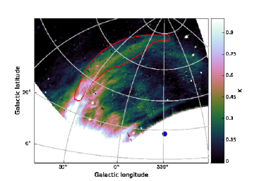
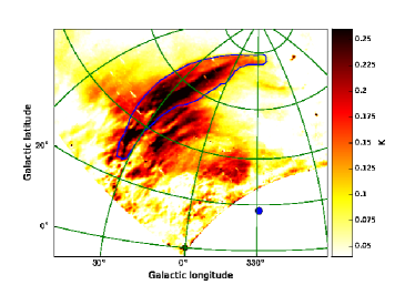
Figure 1.— Images of the total (upper) and polarized (lower) intensity of the NPS averaged between 1.44 and 1.5 GHz. The images are in stereographic projection centered at $(l,\,b)=(329\arcdeg,\,17\fdg 5)$, the center of Loop I (Berkhuijsen et al., 1971), a position marked as a blue dot in each panel. The contour marks the NPS as defined by its polarized intensity. The resolution is $40\arcmin$ and the rms noise is about 20 mK for total intensity and 6 mK for polarized intensity.

We selected a frequency range of 1.44 – 1.5 GHz consisting of 253 channels where there is almost no radio frequency interference and derived the average total intensity ($I_{1.47}$) and polarized intensity ($P_{1.47}$) over this frequency range. The resulting images are shown in Fig. 1 in stereographic projection with the projection center at $(l,\,b)=(329\arcdeg,\,17\fdg 5)$ which is regarded as the center of Loop I (Berkhuijsen et al., 1971). We mark a contour denoting the outer boundary of the NPS on the basis of its morphology as seen in the $P_{1.47}$ image where $P_{1.47}>0.1$ K and RM errors are less than about 5 rad m^-2, as discussed below. The NPS can be clearly identified in both total intensity and polarization. At latitudes higher than about $40\arcdeg$, the inner edge of the NPS is much brighter than the outer edge, which is consistent with previous observations.

For each pixel with a polarized intensity $P_{1.47}$ larger than 0.1 K (about $5\sigma$-level per frequency channel), we linearly fit polarization angles ($\chi$) versus wavelength squared ($\lambda^{2}$) over the entire frequency range from 1280 to 1750 MHz to obtain an RM as

$$\chi(\lambda^{2})=\chi_{0}+{\rm RM}\lambda^{2},$$ (1)

where $\chi_{0}$ is a constant. The map of RMs is shown in Fig. 2 (top panel). We also show the Galactic Faraday depth map constructed by Oppermann et al. (2015) from RMs of extragalactic sources in Fig. 2 (lower panel). Although the linear fitting can also be applied to weaker polarized intensities, larger errors will be introduced, as shown below.

It has been demonstrated that the RM from linearly fitting polarization angle versus $\lambda^{2}$ can be wrong unless the behavior of polarization fraction against $\lambda^{2}$ is examined (Burn, 1966; Farnsworth et al., 2011). In reality, the NPS is either Faraday thin with only synchrotron-emitting medium or Faraday thick with a mixture of synchrotron-emitting and Faraday-rotating medium. For the Faraday thin case, the linear relation between polarization angle and $\lambda^{2}$ always holds. For the Faraday thick case, the linear relation holds for certain ranges of wavelengths and the RMs represent half of the true values (e.g. Sokoloff et al., 1998). For the current data, linear relations between polarization angle and $\lambda^{2}$ can be seen for virtually all the pixels with $P_{1.47}$ larger than 0.1 K. The RMs shown in Fig. 2 (top) are thus reliable.

We also generated an RM map using all data over the entire frequency range of 1280 to 1750 MHz via the RM synthesis method (Brentjens & de Bruyn, 2005). Although the resolution in RM is only 150 rad m^-2, the signal-to-noise is high, allowing measurements of peak RM on finer scales. The resulting RM map is completely consistent with the RM map shown in Fig. 2 (top); the difference between RMs calculated in these two ways has a mean value of $0\pm 1$ rad m^-2 over an area much larger than the NPS. We conclude that the NPS is Faraday thin as the RM synthesis method often fails to reproduce RM when a source is Faraday thick (Sun et al., 2015). The RM map in Fig. 2 (top) is very similar to that obtained by Wolleben et al. (2010b) from RM synthesis based on the pilot GMIMS data, but has higher resolution and sensitivity.

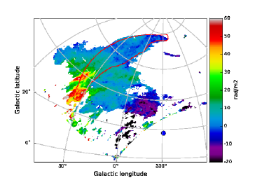
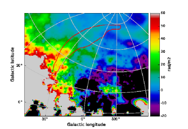
Figure 2.— RM map for the NPS region from GMIMS (upper panel) and the Galactic Faraday depth map constructed by Oppermann et al. (2015) from RMs of extragalactic sources (lower panel). The contours are the same as in Fig. 1.

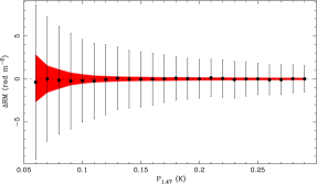
Figure 3.— Difference between the input and fitted RM values, $\Delta{\rm RM}$, versus the polarized intensity averaged over 1.44 – 1.5 GHz, $P_{1.47}$, from faked sources. The red shaded area shows the expected difference at given $P_{1.47}$.

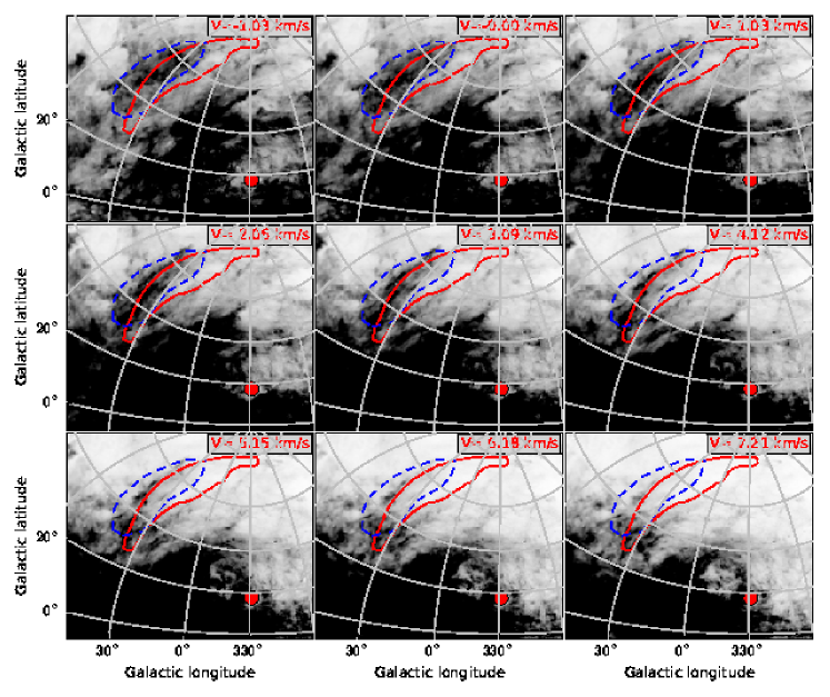
Figure 4.— H i intensity maps from the LAB survey from velocity $-1.03$ km s^-1 to $+$7.21 km s^-1 with a step of 1.03 km s^-1 (from top left to bottom right). The gray scale runs from 0.1 K (white) to 20 K (dark). The NPS is outlined in red solid lines and an H i feature possibly associated with the NPS is outlined in blue dashed lines. The red dots indicate the projection center as in Fig. 1.

The best published RMs for the NPS are those of Spoelstra (1984), based on surveys at 408, 465, 610, 820, and 1411 MHz. Polarization angle measurements, with different beams at these frequencies, were used to compute RM point-by-point; spatial undersampling precluded smoothing to a common beamwidth and computation of an RM map. Because of undersampling in frequency, $|{\rm{RM}}|$ was restricted to values less than ${35~{}{\rm{rad~{}m}}^{-2}}$. The resulting RM “map” is probably sensitive only to spatial scales ${\gtrsim}{\thinspace}{3^{\circ}}$. No useful comparison of our new RMs with these older data is possible.

We made simulations to quantify the RM errors. We extracted a data cube centered at an empty area with a size $\sim 30\arcdeg\times 20\arcdeg$ which contains primarily noise but no polarized structures in any of the frequency channels. For each pixel, we generated a fake source with a randomly selected intrinsic polarization angle, polarized intensity and RM, and added the corresponding $U$ and $Q$ of the source to each individual frequency channel. We then derived a new data cube of polarization angle and applied the same linear fitting procedure as above to calculate a RM map. The difference, $\Delta{\rm RM}$, between the derived RM values and the input RM values provides a robust estimate of the RM errors. We show $\Delta{\rm RM}$ versus $P_{\rm 1.47}$ in Fig. 3. We repeated the process by adding the same fake sources to Gaussian noise with an rms value of 20 mK as measured from the data, which yielded the expected errors (red shaded area in Fig. 3). The real RM errors are much larger than the expected errors. This is probably related to low-level scanning effects in the data; the basket-weaving process reduces such effects, but does not completely remove them. We kept only those pixels with a $P_{\rm 1.47}$ larger than 0.1 K so that the RM errors are lower than about 5 rad m^-2.

Two patches with high positive values can be identified in both the RM and Faraday depth maps in Fig. 2. The one at $b<35\arcdeg$ can be clearly seen in the RM map (upper panel in Fig. 2), but is not especially obvious in the Faraday depth map (lower panel in Fig. 2). In contrast, the other at $36\arcdeg<b<46\arcdeg$ is clearly seen in the Faraday depth map, but has smaller extent in the RM map. Wolleben et al. (2010b) attribute both patches to Faraday rotation by a local H i bubble associated with Upper Scorpius, one of the three subgroups of the Sco-Cen OB association, at a distance of about 145 pc. Towards latitudes above about $50\arcdeg$, which are not influenced by that H i bubble, RMs gradually decrease to zero with large fluctuations.

2.2. H i data revisited

Heiles & Jenkins (1976) claimed that the NPS is associated with H i gas over the velocity range $-$20 km s^-1 to $+$20 km s^-1, using data from the Hat Creek H i survey. Using the Leiden/Argentine/Bonn (LAB) survey (Kalberla et al., 2005), which has much higher sensitivity, we re-investigate the associations between H i gas and the NPS.

By comparing the NPS with each individual velocity channel map from the LAB survey, we find that a filament oriented almost parallel to $l\approx 40\arcdeg$ extending from $b\approx 30\arcdeg$ to $b\approx 70\arcdeg$ over the velocity range from $-$1.03 to $+$7.21 km s^-1 is possibly morphologically associated with the NPS (Fig. 4), consistent with the finding by Heiles & Jenkins (1976). The vertical H i filament can be best seen at velocity $+2.06$ km s^-1, roughly parallel to the NPS, gradually fading away towards velocity $+7.21$ km s^-1 and becoming brighter but mixed with large-scale background emission towards velocity $-1.03$ km s^-1. A contour based on the morphology of the filament at velocity $+2.06$ km s^-1 is shown in each velocity frame in Fig. 4. Because of the high latitude and the very low velocity, the distance to the H i structure cannot be constrained.

We estimate the mass of the H i gas contained in the region within the dashed blue contour of Fig. 4 over the velocity range from $-$1.03 to $+$7.21 km s^-1 to be about $10^{3}D_{100}^{2}$ M_⊙, where $D_{100}$ is the distance to the H i with a nominal value of 100 parsecs. Assuming the H i gas is part of a large shell structure, Weaver (1979) obtained an expansion velocity of 2 km s^-1 which corresponds to a kinetic energy of about $4\times 10^{42}D_{100}^{2}$ ergs. For $D_{100}=1$, the kinetic energy is $4\times 10^{42}$ ergs, which can be easily produced by stellar winds from the Sco-Cen cluster (Weaver, 1979), and for $D_{100}=100$, the kinetic energy of $4\times 10^{46}$ ergs is well below what a nuclear explosion (Sofue, 2000) and galactic winds (Bland-Hawthorn & Cohen, 2003) in the Galactic center can provide. Thus the H i filament can be either local or far away according to the energy budget, and the NPS, if it is associated with the H i filament, can be either local or distant.

2.3. Optical starlight polarization revisited

The light from stars becomes polarized when it is selectively absorbed during propagation by dust grains aligned by the magnetic field (Davis & Greenstein, 1951). Starlight polarization vectors are parallel to the magnetic field in the dust and the polarization fraction depends on the depth of the sightline and on the degree of ordering of the magnetic field perpendicular to the sightline (Fosalba et al., 2002). In contrast, radio polarization vectors, after correction for Faraday rotation, are perpendicular to magnetic field vectors.

Spoelstra (1972) compared the polarization angles of radio emission at 1415 MHz from the NPS with those of optical starlight polarization and found that for stars with distances larger than about 100 pc the two angles differ by about $90\arcdeg$ indicating that they trace the same magnetic field. This set the distance to the NPS at about 100 pc.

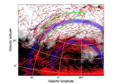
Figure 5.— Optical starlight polarization vectors (red bars) overlaid on the Planck dust image at 353 GHz (Planck Collaboration et al., 2014). The lengths of the bars are proportional to the polarization fraction, and their orientations indicate the orientations of magnetic fields. The green line and blue line outline the NPS and the H i structure described in Sect. 2.2. The two circles are centered at $(l,\,b)=(335\arcdeg,\,10\arcdeg)$ with radii of $35\arcdeg$ and $60\arcdeg$.

There are now more optical polarization data including the compilations by Heiles (2000), Santos et al. (2011) and Berdyugin et al. (2014), which motivate us to re-examine the correlations between starlight polarization and other tracers of the NPS. In Fig. 5 we show optical starlight polarization data overlaid on the Planck dust map (Planck Collaboration et al., 2014).

At latitudes $b>20\arcdeg$ the starlight polarization vectors have a curvature which resembles that of the dust structures (Fig. 5); the curvature of the vectors suggests a center at $(l,\,b)\approx(335\arcdeg,\,10\arcdeg)$. In Fig. 5, we show two partial circles with radii of $35\arcdeg$ and $60\arcdeg$ centered at this position. The starlight polarization vectors are in good alignment with the circles. There appears to be a dust bubble centered at about the same position with a radius of about $30\arcdeg$, but no prominent filamentary structure within this dust bubble.

Berkhuijsen et al. (1971) placed the center of Loop I at $(l,\,b)=(329\arcdeg,\,17.5\arcdeg)$, not far from the center of starlight polarization vectors. It is thus possible that both the NPS and the starlight polarization are products of the same field configuration. The starlight polarization vectors are quite well aligned with the H i feature that we identify in Section 2.2, and, not surprisingly, there appears to be dust associated with the H i as well.

We conclude that the starlight polarization vectors cannot be firmly related to the NPS on the basis of morphology. We turn now to evidence provided by the percentage polarization of the starlight and the relationship between starlight polarization vectors and radio polarization vectors (which should be orthogonal if both polarization signals are from the same magnetic field).

The polarization percentage of the optical starlight polarization versus distance to the stars towards and outside the NPS for $b<40\arcdeg$ and $b>40\arcdeg$ is shown in Fig. 6. Most of the distances are from parallax measurements with accuracy better than 50%. Here “towards” implies the area within the contour denoting the NPS in Figs. 2, and “outside” is defined as the area $10\arcdeg$ outside the contour in Fig. 2. For directions towards the NPS, we also show the polarization angle difference from the WMAP 23 GHz data (Bennett et al., 2013) where Faraday rotation is very small.

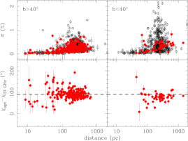
Figure 6.— Polarization percentage of optical starlight and the difference of polarization angles between the optical starlight polarization and WMAP 23 GHz polarization, both as a function of distances. The filled circles (red) are for stars towards the NPS and the open circles (black) are for stars outside the NPS. The dashed lines mark a $90\arcdeg$ polarization angle difference.

For $b>40\arcdeg$, the polarization percentages for stars towards and outside the NPS are very similar, and they both start increasing at distances above 60 pc, reach maximum values between 200 and 300 pc and then slightly decrease up to a distance of 700 pc. This can be interpreted by a continuous distribution of dust over the distance range 60 – 700 pc with the magnetic field inside the dust gradually changing orientation as a function of distance. The angle difference is roughly centered at $90\arcdeg$ for distances larger than about 60 pc, although the scatter is large. This indicates that the NPS traces a similar magnetic field to the dust, and yields a very loose estimate of 60 – 700 pc for the distance to the NPS. It is also possible that the NPS is further with its magnetic field extending from or coincident with the magnetic field in the distance of 60 – 700 pc.

For $b<40\arcdeg$, there are not many polarization measurements for stars towards the NPS. Therefore even a rough estimate of the distance to the NPS is very uncertain, and more data are needed.

3. Discussion

3.1. The location of the NPS

Following Burn (1966) and Brentjens & de Bruyn (2005), we introduce the Faraday depth (FD) as a function of distance along a line of sight, $l$, which is defined as

$${\rm FD}(l)=K\int_{l}^{0}n_{e}(s)B_{\parallel}(s){\rm d}s,$$ (2)

where the integral is along the line of sight, $K$ is a constant, $n_{e}$ is the electron density, $B_{\parallel}$ is the magnetic field projected along the line of sight, and $s$ is the distance increment. For the Faraday depth of the Galaxy ($\rm FD_{G}$), $l$ is the distance from the observer to the edge of the Galaxy. The differential Faraday depth of a source, $\rm\Delta FD$, can then be defined as

$${\rm\Delta FD}={\rm FD}(l_{2})-{\rm FD}(l_{1}),$$ (3)

where $l_{1}$ and $l_{2}$ are the distance of the near and far boundaries of the source, respectively. A detailed discussion of the distinction between RM and FD is given by Sun et al. (2015). Throughout the paper, we use the FD map of the Galaxy which has been constructed by Oppermann et al. (2015) primarily based on the RM catalog by Taylor et al. (2009) and the RMs towards the Galactic poles by Mao et al. (2010). The extended critical filter (Oppermann et al., 2011) was used for the construction, which was able to simultaneously recover the Faraday depth, its angular power spectrum, and the noise co-variance. The minimum scale of the final Faraday depth map can be as small as $0.5\arcdeg$. The typical uncertainty is about 5 rad m^-2 towards latitudes greater than about $40\arcdeg$, and about 10 rad m^-2 towards latitudes between $20\arcdeg$ and $40\arcdeg$. Note that we also tried the FD map of the Galaxy by Xu & Han (2014) for the analysis below and found similar results. The FD map by Oppermann et al. (2015) covering the NPS is presented in the lower panel of Fig. 2.

Our aim is to constrain the location of the NPS by comparing the differential FD of the Galactic ISM in front of the NPS ($\Delta\rm FD_{FG}$) with that of the Galactic ISM behind the NPS through to the edge of the Galaxy ($\Delta\rm FD_{BG}$). The known quantities from observations are the RMs of the NPS ($\rm RM_{NPS}$), the FDs of the Galaxy through ($\rm FD_{G,\,T}$) and outside ($\rm FD_{G,\,O}$) the NPS; and the unknowns are $\rm\Delta FD_{FG}$, $\rm\Delta FD_{BG}$, the differential FD of the NPS itself ($\rm\Delta FD_{NPS}$) and the differential FD of the H i bubble ($\rm\Delta FD_{HI}$). The area of the NPS has been outlined in Fig. 2. We restrict the area outside the NPS to be within $10\arcdeg$ longitude from both sides of the NPS at each latitude. For Galactic latitudes between $28\arcdeg$ and $76\arcdeg$ we average $\rm RM_{NPS}$, $\rm FD_{G,\,T}$, and $\rm FD_{G,\,O}$ in latitude bins of $4\arcdeg$ and over all the corresponding longitudes and obtain their latitude profiles (Fig. 7).

The high positive RMs and FDs that are associated with the local H i bubble in front of the NPS (Wolleben et al., 2010b, and their Figure 3) can be clearly seen in Fig. 2. Because of the influence of this H i bubble, we divided the NPS into two regions:

• $b\lesssim 50\arcdeg$ – The differential FD of the H i bubble in front of the NPS has to be accounted for. We can represent $\rm RM_{NPS}$, $\rm FD_{G,\,T}$ and $\rm FD_{G,\,O}$ as

  $$\left\{\begin{array}[]{rcl}\rm RM_{NPS}&=&\rm\Delta FD_{HI,\,T}+\Delta FD_{FG}+\frac{1}{2}\Delta FD_{NPS}\\[8.53581pt] \rm FD_{G,\,T}&=&\rm\Delta FD_{HI,\,T}+\Delta FD_{FG}+\Delta FD_{NPS}+\Delta FD_{BG}\\[8.53581pt] \rm FD_{G,\,O}&=&\rm\Delta FD_{HI,\,O}+\Delta FD_{FG}+\Delta FD_{BG}.\end{array}\right.$$ (4)

  Here $\rm\Delta FD_{HI,\,T}$ and $\rm\Delta FD_{HI,\,O}$ are the differential FD of the H i bubble covering the NPS and the area outside the NPS, respectively. The factor $\frac{1}{2}$ comes from the assumption that the thermal gas within the NPS is uniformly mixed with non-thermal emitting gas (e.g. Sokoloff et al., 1998). The assumption is reasonable as good linear relations between polarization angles and $\lambda^{2}$ hold towards the NPS.

• $b\gtrsim 50\arcdeg$ – There is no influence by the H i bubble in this region, and $\rm RM_{NPS}$, $\rm FD_{G,\,T}$ and $\rm FD_{G,\,O}$ can be expressed as

  $$\left\{\begin{array}[]{rcl}\rm RM_{NPS}&=&\rm\Delta FD_{FG}+\frac{1}{2}\Delta FD_{NPS}\\[8.53581pt] \rm FD_{G,\,T}&=&\rm\Delta FD_{FG}+\Delta FD_{NPS}+\Delta FD_{BG}\\[8.53581pt] \rm FD_{G,\,O}&=&\rm\Delta FD_{FG}+\Delta FD_{BG}.\end{array}\right.$$ (5)

Figure 7.— Galactic latitude profiles of RM, FD and differential FD. Top panel: the filled (open) circles represent FDs of the Galaxy through (outside) the NPS and the squares represent RMs of the NPS derived from the GMIMS data; Bottom panel: the difference between the FDs through and outside the NPS.

We first estimate the differential FD of the NPS. For the area $b\gtrsim 50\arcdeg$, it can be derived from Eq. (5) as

$$\rm\Delta FD_{NPS}=FD_{G,\,T}-FD_{G,\,O}.$$ (6)

The results are shown in Fig. 7 (bottom panel). The average of $\rm\Delta FD_{NPS}$ is 2$\pm$4 rad m^-2, consistent with zero. This is likely due to the lack of thermal electrons as no excess H$\alpha$ emission can be seen towards the NPS from the composite all-sky H$\alpha$ map of Finkbeiner (2003). For the area $b\lesssim 50\arcdeg$, the differential FD of the NPS can be derived from Eq. (5) as

$$\rm\Delta FD_{NPS}=\rm FD_{G,\,T}-FD_{G,\,O}-(\Delta FD_{HI,T}-\Delta FD_{HI,O}).$$ (7)

The differential FDs of the H i bubble through and outside the NPS are unknown, it is therefore difficult to solve for $\rm\Delta FD_{NPS}$. For the lower part $b\lesssim 36\arcdeg$, $\rm FD_{G,\,T}-FD_{G,\,O}$ is around zero (Fig. 7, bottom panel), which means

$$\rm\Delta FD_{NPS}=\Delta FD_{HI,O}-\Delta FD_{HI,T}.$$ (8)

There is no physical connection between the NPS and the H i bubble and hence no relation between $\rm\Delta FD_{NPS}$ and $\rm FD_{HI,O}-FD_{HI,T}$. This implies that both sides of Eq. (8) are equal to zero for the latitude range $b\lesssim 36\arcdeg$. Since $\rm\Delta FD_{NPS}$ is close to zero towards both larger and smaller Galactic latitudes, we assume it is also close to zero towards the middle part $36\lesssim b\lesssim 50\arcdeg$. This can be corroborated by the fact that the patch with high positive RM crosses the eastern edge of the NPS without any change (Fig. 2). The large values of $\rm FD_{G,\,T}-FD_{G,\,O}$ for $36\lesssim b\lesssim 50\arcdeg$ (Fig. 7) can be attributed to the large difference between $\rm\Delta FD_{HI,T}$ and $\rm\Delta FD_{HI,O}$ which can also be seen from Fig. 2. For the discussions below, we assume $\rm\Delta FD_{NPS}$ is zero for $b\lesssim 50\arcdeg$.

We now look at $\rm\Delta FD_{BG}$ and $\rm\Delta FD_{FG}$. For the entire latitude range, we can obtain an estimate of $\rm\Delta FD_{BG}$ from Eqs. (4) and (5) as,

$$\rm\Delta FD_{BG}=\rm FD_{G,T}-RM_{NPS}-\frac{1}{2}\Delta FD_{NPS}.$$ (9)

From previous discussions, $\rm\Delta FD_{NPS}$ is zero, and $\rm\Delta FD_{BG}$ can then be derived. The resulting profile of $\rm\Delta FD_{BG}$ is shown in Fig. 8. We can only solve $\rm\Delta FD_{FG}$ for the latitude range $b\gtrsim 50\arcdeg$ from Eq. (5) as

$$\rm\Delta FD_{FG}=RM_{NPS}-\frac{1}{2}\Delta FD_{NPS},$$ (10)

and the result is shown in Fig. 8.

Figure 8.— $\rm FD_{FG}$ and $\rm FD_{BG}$ versus Galactic latitude. The lower solid and dashed lines are from the models by Sun & Reich (2010) and Jansson & Farrar (2012), respectively. The upper solid line is from the model by Sun & Reich (2010) but with an extra dipole field with a strength of 0.2 $\mu$G at the Sun’s position.

For the area $b\gtrsim 50\arcdeg$, $\rm\Delta FD_{FG}$ is consistent with 0 rad m^-2. Since $\rm\Delta FD_{BG}$ is not zero, a regular magnetic field and constant thermal electron density must exist along the entire line of sight. In this case, $\rm\Delta FD_{FG}$ values of zero imply that the path length in the integral in Eq. (2) is close to zero and the NPS is thus a local feature. From the 3D modeling of the ISM by Puspitarini et al. (2014), the local cavity, defined as an irregularly shaped area of very low density gas surrounding the Sun, extends to about 100 pc towards the NPS. From Fig. 6, dust starts to appear only from the distance further than about 60 pc, which supports the existence of the local cavity. Within the cavity, the differential FD must be around zero, and any contributions to Faraday depths start beyond the cavity wall. Since the Galactic magnetic field is predominately parallel to the plane (e.g. Sun et al., 2008, and references therein), the line of sight component of magnetic field towards latitudes higher than $50\arcdeg$ is very low. The contributions to Faraday depths thus increase very slowly as a function of distance. All these considerations place the NPS at a distance of several hundred parsecs.

Towards latitudes $b\lesssim 50\arcdeg$, $\rm\Delta FD_{BG}$ increases with latitude from a value of $-11$ rad m^-2 at $b=28\arcdeg$ to 17 rad m^-2 at $b=44\arcdeg$, and decreases towards higher latitudes. There are two possible explanations for the behavior of $\rm\Delta FD_{BG}$. One is that the NPS is local and $\rm\Delta FD_{BG}$ is from the large-scale Galactic magnetic field which has a change of sign at $b=44\arcdeg$. The other is that the low latitude part and the high latitude part of the NPS are separate structures. It can be seen from the total intensity image in Fig. 1 that the low latitude part is much brighter than the high latitude part and the transition is not smooth, which can also be seen from the recent all-sky radio continuum map at 1.4 GHz by Calabretta et al. (2014). The comparison of polarization observations at 2.3 and 4.8 GHz indicates that the very low latitude part is further than 2 – 3 kpc (Sun et al., 2014). With the low latitude part of the NPS far away, the path length from the NPS to the edge of the Galaxy is largely reduced and thus $\rm\Delta FD_{BG}$ is much less than that extrapolated from high latitudes.

3.2. Modeling of the Galactic magnetic field

Modeling of the large-scale magnetic field in the Galaxy is very challenging. Ideally models should be able to reproduce a broad range of observations such as the FD of the Galaxy, including the total intensity and polarized intensity from the synchrotron emission. Both Sun & Reich (2010) and Jansson & Farrar (2012) have built models of the Galactic magnetic field, including both disk and halo components.

The differential FD of the Galactic ISM behind the NPS for $b\gtrsim 50\arcdeg$ is almost equal to the FD of the Galaxy, which allows us to test the models of Sun & Reich (2010) and Jansson & Farrar (2012). In Fig. 8, we show the FD profile of the Galaxy from both these Galactic magnetic field models. Both models predict a FD smaller than $\rm\Delta FD_{BG}$. To increase FDs, the models need to have a larger magnetic field along line of sight, which can be achieved by increasing either magnetic field parallel to the Galactic plane or magnetic field perpendicular to the Galactic plane. From Fig. 8, it can be seen that $\rm\Delta FD_{BG}$ tends to be constant at a value around $+$3 rad m^-2 for latitudes higher than about $60\arcdeg$, consistent with the value obtained by Taylor et al. (2009) from NVSS RMs for area $76\arcdeg<b<90\arcdeg$. The magnetic field parallel to the Galactic plane cannot contribute FD towards the north Galactic pole. Therefore, a vertical component must be incorporated to explain the $\rm\Delta FD_{BG}$, which is not included in the model of Sun & Reich (2010) and seems insufficient with the X-shape magnetic field in the model of Jansson & Farrar (2012).

To demonstrate the necessity of a vertical magnetic field, we tried to add a dipole magnetic field component to the model by Sun & Reich (2010). We find that with a field strength of 0.2 $\mu$G and a direction pointing from the north Galactic pole towards the observer at the position of the Sun, the revised model can now reproduce $\rm\Delta FD_{BG}$ for $b\gtrsim 50\arcdeg$ (Fig. 8).

There is uncertainty in constraining large-scale magnetic field models with $\rm FD_{BG}$ at $b\lesssim 50\arcdeg$. If the NPS is local, the models by Sun & Reich (2010) and Jansson & Farrar (2012) both fail to reproduce $\rm\Delta FD_{BG}$. In this case, the differential FD of the H i bubble dominates the FD of the inner Galaxy, producing the mistaken appearance of an anti-symmetric pattern of FDs between the first and fourth Galactic quadrants. Sun & Reich (2010) incorporated this anti-symmetric pattern into their overall Galactic magnetic field model. Subsequently, Wolleben et al. (2010b) highlighted that much of this pattern was due to the H i bubble, which led Jansson & Farrar (2012) to subtract its contribution to FD when modeling the Galactic magnetic field. However, there still remain high FDs towards the NPS around $b=30\arcdeg$ in the bottom panel of their Figure 1 after the subtraction, which is not consistent with our results in Fig. 8. Our work demonstrates that there is no evidence for this anti-symmetric pattern in the large-scale FD of the Milky Way at least around $b=30\arcdeg$ if the NPS is local.

4. Conclusions

The North Polar Spur (NPS), one of the largest coherent structures in the radio sky, has been known for more than half a century. The nature of the NPS still remains controversial: is it a local supernova remnant or a Galactic scale feature related with a starburst or a bipolar wind from the Galactic center? We find that it can be both.

The key to understanding the nature of the NPS is its location in the Galaxy, and this has been the focus of our paper. We employed recent H i and starlight polarization data and found that neither of these datasets can give an exact distance to the NPS, or to the dust structure within the NPS perimeter. We then turned to the polarization data from GMIMS for a possible constraint of the distance to the NPS.

GMIMS provides an unprecedented data set with about 2000 frequency channels at 1.3 – 1.8 GHz. Taking advantage of the multi-channel data, we were able to obtain an RM map of the NPS by linearly fitting the polarization angle versus wavelength squared. Based on the RM map of the NPS and the FD map of the Galaxy, we derived the differential Faraday depth of the NPS, the differential Faraday depth of the Galactic interstellar medium in front of the NPS and the differential Faraday depth of the Galactic interstellar medium behind the NPS through to the edge of the Galaxy for the Galactic latitude range $28\arcdeg<b<76\arcdeg$.

We argue that the part of the NPS at $b\gtrsim 50\arcdeg$ is local at a distance of about several hundred parsecs because the differential Faraday depth of the Galactic ISM in front of the NPS is around zero. This part of the NPS is probably embedded in a large local magnetic field bubble that is traced by starlight polarization. With decreasing latitude, differential Faraday depth behind the NPS gradually increases, reaches a maximum at $b=44\arcdeg$, and then slowly decreases. This implies that either the NPS at $b<44\arcdeg$ is far away or the NPS is local but the large-scale magnetic field has a sign change. If the NPS is local, the large positive Faraday depths are contributed by an H i bubble in front of the NPS, and the large-scale anti-symmetric pattern in Faraday depth is then not contributed by a large-scale magnetic field.

We show that the Galactic magnetic field models by Sun & Reich (2010) and Jansson & Farrar (2012) cannot reproduce the differential Faraday depth behind the NPS at $b>50\arcdeg$. We find that the model by Sun & Reich (2010) plus a dipole magnetic field with a direction pointing from the north to the south Galactic pole and a strength of 0.2 $\mu$G at the Sun’s position can explain the differential Faraday depth behind the NPS. This demonstrates that there exists a coherent large-scale vertical magnetic field in the Galaxy near the Sun’s position, which should be taken into account in future modeling of Galactic magnetic fields.

The location of the NPS is uncertain because the differential Faraday depth in front of the NPS cannot be solved at $b\lesssim 50\arcdeg$ due to the contamination of a local H i bubble in front of the NPS. Future polarimetric observations at lower frequencies that provide a higher resolution in Faraday depth are needed to properly account for the Faraday depth of the H i bubble.

References

- Axon & Ellis (1976) Axon, D. J., & Ellis, R. S. 1976, MNRAS, 177, 499
- Bennett et al. (2013) Bennett, C. L., Larson, D., Weiland, J. L., et al. 2013, ApJS, 208, 20
- Berdyugin et al. (2014) Berdyugin, A., Piirola, V., & Teerikorpi, P. 2014, A&A, 561, A24
- Berkhuijsen et al. (1971) Berkhuijsen, E. M., Haslam, C. G. T., & Salter, C. J. 1971, A&A, 14, 252
- Bland-Hawthorn & Cohen (2003) Bland-Hawthorn, J., & Cohen, M. 2003, ApJ, 582, 246
- Brentjens & de Bruyn (2005) Brentjens, M. A., & de Bruyn, A. G. 2005, A&A, 441, 1217
- Bunner et al. (1972) Bunner, A. N., Coleman, P. L., Kraushaar, W. L., & McCammon, D. 1972, ApJ, 172, L67
- Burn (1966) Burn, B. J. 1966, MNRAS, 133, 67
- Calabretta et al. (2014) Calabretta, M. R., Staveley-Smith, L., & Barnes, D. G. 2014, PASA, 31, 7
- Colomb et al. (1980) Colomb, F. R., Poppel, W. G. L., & Heiles, C. 1980, A&AS, 40, 47
- Davis & Greenstein (1951) Davis, Jr., L., & Greenstein, J. L. 1951, ApJ, 114, 206
- Egger & Aschenbach (1995) Egger, R. J., & Aschenbach, B. 1995, A&A, 294, L25
- Farnsworth et al. (2011) Farnsworth, D., Rudnick, L., & Brown, S. 2011, AJ, 141, 191
- Finkbeiner (2003) Finkbeiner, D. P. 2003, ApJS, 146, 407
- Fosalba et al. (2002) Fosalba, P., Lazarian, A., Prunet, S., & Tauber, J. A. 2002, ApJ, 564, 762
- Guzmán et al. (2011) Guzmán, A. E., May, J., Alvarez, H., & Maeda, K. 2011, A&A, 525, A138
- Hanbury Brown et al. (1960) Hanbury Brown, R., Davies, R. D., & Hazard, C. 1960, The Observatory, 80, 191
- Heiles (2000) Heiles, C. 2000, AJ, 119, 923
- Heiles & Jenkins (1976) Heiles, C., & Jenkins, E. B. 1976, A&A, 46, 333
- Jansson & Farrar (2012) Jansson, R., & Farrar, G. R. 2012, ApJ, 757, 14
- Kalberla et al. (2005) Kalberla, P. M. W., Burton, W. B., Hartmann, D., et al. 2005, A&A, 440, 775
- Kataoka et al. (2013) Kataoka, J., Tahara, M., Totani, T., et al. 2013, ApJ, 779, 57
- Lallement et al. (2014) Lallement, R., Vergely, J.-L., Valette, B., et al. 2014, A&A, 561, A91
- Large et al. (1966) Large, M. I., Quigley, M. F. S., & Haslam, C. G. T. 1966, MNRAS, 131, 335
- Mao et al. (2010) Mao, S. A., Gaensler, B. M., Haverkorn, M., et al. 2010, ApJ, 714, 1170
- Miller et al. (2008) Miller, E. D., Tsunemi, H., Bautz, M. W., et al. 2008, PASJ, 60, 95
- Oppermann et al. (2011) Oppermann, N., Robbers, G., & Enßlin, T. A. 2011, Phys. Rev. E, 84, 041118
- Oppermann et al. (2015) Oppermann, N., Junklewitz, H., Greiner, M., et al. 2015, A&A, 575, A118
- Planck Collaboration et al. (2014) Planck Collaboration, Ade, P. A. R., Aghanim, N., et al. 2014, A&A, 571, A12
- Puspitarini et al. (2014) Puspitarini, L., Lallement, R., Vergely, J.-L., & Snowden, S. L. 2014, A&A, 566, A13
- Reich & Reich (1988) Reich, P., & Reich, W. 1988, A&AS, 74, 7
- Roger et al. (1999) Roger, R. S., Costain, C. H., Landecker, T. L., & Swerdlyk, C. M. 1999, A&AS, 137, 7
- Salter (1983) Salter, C. J. 1983, BASI, 11, 1
- Santos et al. (2011) Santos, F. P., Corradi, W., & Reis, W. 2011, ApJ, 728, 104
- Snowden et al. (1997) Snowden, S. L., Egger, R., Freyberg, M. J., et al. 1997, ApJ, 485, 125
- Sofue (2000) Sofue, Y. 2000, ApJ, 540, 224
- Sofue (2015) —. 2015, MNRAS, 447, 3824
- Sokoloff et al. (1998) Sokoloff, D. D., Bykov, A. A., Shukurov, A., et al. 1998, MNRAS, 299, 189
- Spoelstra (1972) Spoelstra, T. A. T. 1972, A&A, 21, 61
- Spoelstra (1984) Spoelstra, T. A. T. 1984, A&A, 135, 238
- Su et al. (2010) Su, M., Slatyer, T. R., & Finkbeiner, D. P. 2010, ApJ, 724, 1044
- Sun et al. (2014) Sun, X. H., Gaensler, B. M., Carretti, E., et al. 2014, MNRAS, 437, 2936
- Sun & Reich (2010) Sun, X. H., & Reich, W. 2010, RAA, 10, 1287
- Sun et al. (2008) Sun, X. H., Reich, W., Waelkens, A., & Enßlin, T. A. 2008, A&A, 477, 573
- Sun et al. (2015) Sun, X. H., Rudnick, L., Akahori, T., et al. 2015, AJ, 149, 60
- Taylor et al. (2009) Taylor, A. R., Stil, J. M., & Sunstrum, C. 2009, ApJ, 702, 1230
- Weaver (1979) Weaver, H. 1979, in IAU Symposium, Vol. 84, The Large-Scale Characteristics of the Galaxy, ed. W. B. Burton (D. Reidel Publishing Co., Dordrecht), 295–298
- Willingale et al. (2003) Willingale, R., Hands, A. D. P., Warwick, R. S., Snowden, S. L., & Burrows, D. N. 2003, MNRAS, 343, 995
- Wolleben (2007) Wolleben, M. 2007, ApJ, 664, 349
- Wolleben et al. (2010a) Wolleben, M., Landecker, T. L., Hovey, G. J., et al. 2010a, AJ, 139, 1681
- Wolleben et al. (2010b) Wolleben, M., Fletcher, A., Landecker, T. L., et al. 2010b, ApJ, 724, L48
- Xu & Han (2014) Xu, J., & Han, J.-L. 2014, Research in Astronomy and Astrophysics, 14, 942