Geometry of reduced density matrices for symmetry-protected topological phases

Abstract

In this paper, we study the geometry of reduced density matrices for states with symmetry-protected topological (SPT) order. We observe ruled surface structures on the boundary of the convex set of low dimension projections of the reduced density matrices. In order to signal the SPT order using ruled surfaces, it is important that we add a symmetry-breaking term to the boundary of the system—no ruled surface emerges in systems without boundary or when we add a symmetry-breaking term representing a thermodynamic quantity. Although the ruled surfaces only appear in the thermodynamic limit where the ground-state degeneracy is exact, we analyze the precision of our numerical algorithm and show that a finite system calculation suffices to reveal the ruled surface structures.

I Introduction

The idea of reading physical properties from the geometry of the underlying convex bodies arising naturally from quantum many-body physics has been examined and re-examined many times from different perspectives in the literature Col63 ; Erd72 ; EJ00 ; VC06 ; GM06 ; SM09 . It appeared in the context of the $N$-representability problem in quantum chemistry and, more generally, the quantum marginal problem in quantum information theory Col63 ; klyachko2006quantum . Recently, the approach received revived interests and was used in the investigations of quantum phases from the convex geometry of reduced density matrices or their low dimension projections EJ00 ; VC06 ; GM06 ; SM09 ; chen2014principle .

Consider a many-body local Hamiltonian $H=\sum_{j}H_{j}$ where each term $H_{j}$ acts non-trivially on a set of particles $S_{j}$. Usually, each $S_{j}$ contains only a constant number of neighboring particles and defines the geometry of the local interactions of the system. The convex set (a convex set in Euclidean space is the region that, for every pair of points within the region, every point on the straight line segment that joins the pair of points is also within the region. For instance, a solid sphere forms a convex set) of quantum marginals, the collections of reduced density matrices $(\rho_{j})$, is of fundamental importance to quantum many-body physics. Here, each $\rho_{j}$ in the same tuple is the reduced state on $S_{j}$ of a common many-body state. The convex set of quantum marginals is independent of the particular form of the Hamiltonian $H$, but depends only on the geometric locality of the system defined by $S_{j}$’s. Should we have a complete characterization of the quantum marginals, most problems of many-body physics would become extremely easy. As expected, however, the structure of the set of quantum marginals is rather complicated.

To study quantum phase transitions, it seems appropriate to investigate a further coarse-grained set of the quantum marginals. The usual situation one often faces when considering quantum phase transitions at zero temperature is the following: the Hamiltonian of the system has the form $H=J_{1}H_{1}+J_{2}H_{2}$ and one is concerned with the change of the properties of lower energy states of $H$ as $J_{1}$ and $J_{2}$ change. The terms $H_{1}$ and $H_{2}$ now act on a large number of particles, but they are still sums of local terms. Let the convex set $\Theta(\{H_{j}\})\subseteq\mathbb{R}^{2}$ be the set of all points $(\operatorname{tr}(H_{1}\rho),\operatorname{tr}(H_{2}\rho))$ for $\rho$ ranging in the set of all possible many-body states. This set is a low dimension projection of the convex set of quantum marginals and is hopefully much easier to analyze.

It is obvious that for any $(\alpha_{1},\alpha_{2})$ in $\Theta(\{H_{j}\})$, $\sum_{i}J_{i}\alpha_{i}\geq E_{0}(H)$, the ground state energy of $H$. This means that the Hamiltonian $H$ can be thought of as the supporting hyperplane of $\Theta(\{H_{j}\})$, and the change of parameters $J_{1},J_{2}$ can be visualized as the change of the supporting hyperplane, moving around the convex set. The intersection of this hyperplane with $\Theta(\{H_{j}\})$ corresponds to the image of the ground state of $H$ on the boundary of $\Theta(\{H_{j}\})$. A flat portion on the boundary of $\Theta(\{H_{j}\})$ signatures the first-order phase transition. However, for continuous phase transitions, the geometry of $\Theta(\{H_{j}\})$ alone does not convey any informative signals chen2014principle .

Recently, the convex geometry approach was employed in the study of quantum symmetry-breaking phases zauner2014symmetry . For a Hamiltonian $H=J_{1}H_{1}+J_{2}H_{2}$ with certain symmetry, one adds a third, symmetry-breaking, term $H_{3}$ to the Hamiltonian and consider $H=J_{1}H_{1}+J_{2}H_{2}+J_{3}H_{3}$. The authors plotted the convex set $\Theta(\{H_{j}\})\subseteq\mathbb{R}^{3}$ of points $(\operatorname{tr}(H_{1}\rho),\operatorname{tr}(H_{2}\rho),\operatorname{tr}(H_{3}\rho))$ and analyzed the geometry of its boundary. On this set, the emergence of ruled surfaces on the boundary is observed (a ruled surface is a surface that can be swept out by moving a line in space, or equivalently, for any point on the ruled surface there exists a line passing through this point that is also on the surface. For example, the curved boundary of a cylinder is a ruled surface). The authors of zauner2014symmetry argued that the existence of those ruled surfaces is a defining property of symmetry-breaking and can be used to signal symmetry-breaking phase transition.

Interestingly, the observation that ruled surfaces on the boundary of certain convex body can explain phase transitions dates back to Gibbs in the 1870’s Gib73a ; Gib73b ; Gib75 ; Isr79 , even though the convex bodies under consideration in classical thermodynamics and quantum many-body physics are rather different. It indicates that the convex geometry approach is a rather fundamental and universal idea.

In the present paper, we study the phenomenon of the emergence of ruled surface on the boundary of the convex set $\Theta(\{H_{j}\})\subseteq\mathbb{R}^{3}$ for one dimensional (1D) symmetry-protected topological (SPT) ordered systems. An SPT ordered state is a bulk-gapped short-range entangled state with symmetry protected nontrivial boundary excitations GW0931 . The well known two dimensional and three dimensional topological insulators KM0501 ; BZ0602 ; KM0502 ; MB0706 ; FKM0703 ; QHZ0824 are free fermion SPT phase protected by time reversal and $U(1)$ charge conservation symmetry, whose boundary remain gapless as long as the symmetries are preserved. SPT phases also exist in interacting systems. A typical example of interacting bosonic SPT phase is the 1D spin-1 Haldane chain H8350 ; H8364 ; AKL8877 ; GW0931 ; PBT0959 , whose degenerate edge states are protected by time reversal, or spatial inversion, or $Z_{2}\times Z_{2}$ spin rotation symmetry GW0931 ; PBT0959 . Bosonic SPT phases can be partially classified by group cohomology theory CGL1314 ; CGLW2012 . Especially, in 1D (which we will study in this paper), SPT phases with onsite-symmetry are classified by $\mathcal{H}^{2}(G,U(1))$, or the projective representations of the symmetry group $G$ ChenGuWen2011_1D ; ChenGuWen2011_1Dfull ; Cirac2011 .

The ground-state degeneracy is a necessary condition for the existence of a ruled surface. However, in order to observe such a ruled surface, we need to add a local term that can lift the degeneracy. In other words, ground-state degeneracy that can be lifted by some local term will lead to ruled surfaces. It is then required such a local term exists. In case of the symmetry-breaking order, it corresponds to the local order parameter. We show that in case of the SPT order, the emergence of a ruled surface only exists for system under open boundary condition (OBC), with the corresponding local term acting on the boundary that breaks the symmetry of the system, hence lifting the ground-state degeneracy.

To show this, we study a 1D model exhibiting $Z_{2}\times Z_{2}$ SPT order. We discuss in detail the effect of geometric locality and its relationship to the emergence of ruled surfaces. Since the degeneracy of the ground states is only exact in thermodynamic limit, in principle the ruled surface also requires such a limit. However, numerical results suggest that in practice, the ruled surface can already be observed for large but finite systems. This allows us to study the features of ruled surface based on finite-system calculations.

One important difference between our results and Ref. zauner2014symmetry is that the boundary terms that lift the degeneracy are not associated with thermodynamic variables. It is essentially the effect of geometric locality (i.e. boundary conditions do change the geometric locality of the system) that leads to a different geometry of the set of reduced density matrices. On the contrary, for a topological ordered system, no local terms can lift the topological degeneracy; therefore one cannot observe ruled surface on the geometry of local reduced density matrices. Our results hence lead to a deeper understanding of the physical meaning of the emergence of ruled surface.

II $Z_{2}\times Z_{2}$ SPT order: The 1D cluster state in magnetic fields

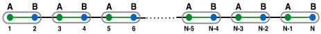
(a)

(b)

Figure 1: 1D system with A, B sublattice. The number of sites $N$ is even. Green and blue dots represent sublattice A and B, respectively. Each small circle represents a unit cell. (a) is the 1D system under open boundary condition and (b) is the system under periodic boundary condition.

Consider a 1D system with A, B sublattice under OBC, see Fig. 1(a). Assuming the number of sites $N$ is even, the Hamiltonian reads:

$$H_{clu}(B_{z})=\sum_{i=2}^{N-1}X_{i-1}Z_{i}X_{i+1}+B_{z}\sum_{i=1}^{i=N}Z_{i},$$ (1)

where $X,Z$ are Pauli operators.

The first term $X_{i-1}Z_{i}X_{i+1}$ corresponds to the stabilizer generators of the $1D$ cluster state (without boundary terms) briegel2001persistent ; raussendorf2001one . The second term corresponds to a longitudinal magnetic field. Notice that $H_{clu}$ has a $Z_{2}\times Z_{2}$ symmetry generated by the following two operators (see e.g. else2012symmetry ; skrovseth2009phase ; doherty2009identifying ),

$$O_{1} =Z_{1}Z_{3}Z_{5}...Z_{N-1}$$ (2)

$$O_{2} =Z_{2}Z_{4}Z_{6}...Z_{N}$$ (3)

Obviously, $[O_{1},O_{2}]=0$ and $[O_{1},H_{clu}]=0,[O_{2},H_{clu}]=0$. In fact, there is also a hidden continuous $U(1)$ symmetry in $H_{clu}$ generated by $\sum_{i=1,odd}^{i=N-1}Y_{i}X_{i+1}-X_{i}Y_{i+1}$.

When $B_{z}<1$, the ground state of above model has $Z_{2}\times Z_{2}$ SPT order. To show this, we can transform $H_{clu}$ into a familiar form with only two-body interactions zeng2014topological . Consider unitary operations $U_{AB}$ acting on each nearest A-B sites, as denoted in Fig.1. Each $U_{AB}$ transform Pauli operators as follows:

$$X_{A} \to X_{A}, Z_{A} \to Z_{A}X_{B},$$ (4)

$$X_{B} \to X_{B}, Z_{B} \to X_{A}Z_{B}.$$ (5)

In fact, $U_{AB}$ is nothing but the controlled-$Z$ operation (i.e. $CZ=\text{diag}(1,1,1,-1)$) in the Pauli $X$ basis (i.e. $\frac{1}{\sqrt{2}}(|0\rangle\pm|1\rangle)$). That is, $U_{AB}=(H_{A}\otimes H_{B})CZ_{AB}(H_{A}\otimes H_{B})$, where $H$ is the Hadamard transformation given by $HXH=Z$.

Under this transformation, we have

$$X_{i-1}^{B}Z_{i}^{A}X_{i+1}^{B}\to X_{i-1}^{B}Z_{i}^{A}$$ (6)

$$X_{i-2}^{A}Z_{i-1}^{B}X_{i}^{A}\to Z_{i-1}^{B}X_{i}^{A}$$ (7)

and

$$Z_{i}^{A}\to Z_{i}^{A}X_{i+1}^{B}$$ (8)

$$Z_{i+1}^{B}\to X_{i}^{A}Z_{i+1}^{B}.$$ (9)

Thus we can recast the original Hamiltonian as following:

$$\begin{split}H_{OBC}&=J_{1}(1+\alpha)\sum_{i=2,even}^{N-2}(X_{i}Z_{i+1}+Z_{i}X_{i+1})\\ &+J_{2}(1-\alpha)\sum_{i=1,odd}^{N-1}(X_{i}Z_{i+1}+Z_{i}X_{i+1}).\\ \end{split}$$ (10)

For the convenience of later calculation, we let $J_{1}=\pm 1$, $J_{2}=\pm 1$, $-1\leq\alpha\leq 1$. If we further apply an unitary transformation on the A sublattice such that

$$X_{i}^{A}\to Z_{i}^{A},\ \ Z_{i}^{A}\to X_{i}^{A},$$

then the model (10) becomes the familiar XY model Perk1 ; Perk2 ; Perk3 ; Perk4 ,

$$\begin{split}H_{OBC}&=J_{1}(1+\alpha)\sum_{i=2,even}^{N-2}(X_{i}X_{i+1}+Z_{i}Z_{i+1})\\ &+J_{2}(1-\alpha)\sum_{i=1,odd}^{N-1}(X_{i}X_{i+1}+Z_{i}Z_{i+1}).\end{split}$$ (11)

The $Z_{2}\times Z_{2}$ symmetry becomes very clear in above Hamiltonian: it is generated by the uniform $X$ and $Z$ operations. Since in the above model each unit cell contains two spins, the strong bonds may locate inter unit cells or intra unit cells, and consequently there are two different phases. When $0<\alpha\leq 1$, the ground state carries nontrivial $Z_{2}\times Z_{2}$ SPT order and has two-fold degenerate edge states (which carry projective representation $\{I,X,Y,Z\}$ of $Z_{2}\times Z_{2}$ group) on each boundary; on the contrary, when $-1\leq\alpha<0$, the model falls in a trivial symmetric phase without edge states; $\alpha=0$ corresponds to the phase transition point. The previously mentioned $U(1)$ continuous symmetry is generated by $\sum_{i}Y_{i}$ in Eq. (11). The $U(1)$ symmetry is an accidental symmetry for the SPT order, namely, the properties of the two phase remains unchanged if the $U(1)$ symmetry is destroyed by anisotropic interactions.

In later discussion, we will go back to the original cluster model. For the purpose of studying the reduced density matrix, we further add a transverse magnetic field. We will consider cases with both OBC and periodic boundary condition (PBC) . Thus under OBC (see Fig. 1(a)), the Hamiltonian reads:

$$\begin{split}H_{OBC}&=J_{1}(1+\alpha)\sum_{i=2}^{N-1}X_{i-1}Z_{i}X_{i+1}\\ &+J_{2}(1-\alpha)\sum_{i=1}^{N}Z_{i}-B_{x}\sum_{i=1}^{N}X_{i}\\ &=J_{1}(1+\alpha)H^{O}_{1}+J_{2}(1-\alpha)H^{O}_{2}-B_{x}H_{3},\\ \end{split}$$ (12)

while under PBC (see Fig. 1(b)), the Hamiltonian is:

$$\begin{split}H_{PBC}&=J_{1}(1+\alpha)\sum_{i=2}^{N+1}X_{i-1}Z_{i}X_{i+1}\\ &+J_{2}(1-\alpha)\sum_{i=1}^{N}Z_{i}-B_{x}\sum_{i=1}^{N}X_{i}\\ &=J_{1}(1+\alpha)H^{P}_{1}+J_{2}(1-\alpha)H^{P}_{2}-B_{x}H_{3},\\ \end{split}$$ (13)

where the $(N+1,N+2)$ sites are identified with the $(1,2)$ sites, respectively.

III Effect of locality and the emergence of ruled surface for SPT phase

One necessary condition for the emergence of a ruled surface is the ground-state degeneracy. When $B_{x}=0,(J_{1},J_{2})=(\pm 1,\pm 1),0<\alpha\leq 1$, the ground-state of $H_{OBC}$ is four-fold degenerate (if $N\to\infty$) and the ground state of $H_{PBC}$ is unique. One may expect that a ruled surface will appear on the surface of the convex set $\Theta(\{H_{j}\})$ consisting of all the points given by

$$\left(\frac{1}{N-2}\operatorname{tr}(H^{O}_{1}\rho),\frac{1}{N}\operatorname{tr}(H^{O}_{2}\rho),\frac{1}{N}\operatorname{tr}(H_{3}\rho)\right)$$ (14)

for any quantum state $\rho$, similar as the symmetry-breaking case as discussed in zauner2014symmetry .

Unfortunately, it is not the case for the SPT order. This is because that the expectation value of the symmetry-breaking term $H_{3}/N$ is mainly contributed from the bulk and the ruled surfaces which result from the edge states will become invisible. This is essentially the meaning of ‘topological’ for the SPT orders, in contrast to symmetry breaking orders. If one instead takes the expectation value of $H_{3}$, which is indeed different for the degenerate ground states, the set

$$\left(\frac{1}{N-2}\operatorname{tr}(H^{O}_{1}\rho),\frac{1}{N}\operatorname{tr}(H^{O}_{2}\rho),\operatorname{tr}(H_{3}\rho)\right),$$ (15)

which is indeed convex, will be unbounded. Furthermore, if one only takes the expectation value on the boundary, i.e. to consider

$$\left(\frac{1}{N-2}\operatorname{tr}(H^{O}_{1}\rho),\frac{1}{N}\operatorname{tr}(H^{O}_{2}\rho),\operatorname{tr}((X_{1}+X_{N})\rho)\right),$$ (16)

then this set is no longer convex (see Appendix A for more details).

To overcome all these difficulties, we instead add the symmetry-breaking term on the boundary of the system. This is because that the degeneracy essentially comes from the edge spins. We therefore propose to use the following Hamiltonian:

$$\begin{split}H_{OBC}&=J_{1}(1+\alpha)H^{O}_{1}+J_{2}(1-\alpha)H^{O}_{2}\\ &-B_{x}(X_{1}+X_{N})\end{split}$$ (17)

And for comparison purpose, we also modify the PBC Hamiltonian to be:

$$\begin{split}H_{PBC}&=J_{1}(1+\alpha)H^{P}_{1}+J_{2}(1-\alpha)H^{P}_{2}\\ &-B_{x}(X_{1}+X_{N})\end{split}$$ (18)

For OBC, the convex set $\Theta(\{H_{j}\})$ can be generated by the following expectation value with respect to the ground state:

$$\langle XZX\rangle=\langle H^{O}_{1}\rangle/(N-2),$$ (19)

$$\langle Z\rangle=\langle H^{O}_{2}\rangle/N,$$ (20)

$$\langle X\rangle=\langle X_{1}+X_{N}\rangle/2.$$ (21)

For PBC, the corresponding quantities are:

$$\langle XZX\rangle=\langle H^{P}_{1}\rangle/N,$$ (22)

$$\langle Z\rangle=\langle H^{P}_{2}\rangle/N,$$ (23)

$$\langle X\rangle=\langle X_{1}+X_{N}\rangle/2.$$ (24)

We show that there will then be emergence of ruled surfaces on the boundary of $\Theta(\{H_{j}\})$ for OBC, and no ruled surfaces for PBC, which is illustrated in Fig. 2.

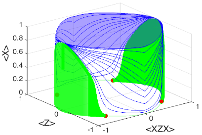
(a)

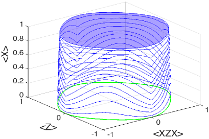
(b)

Figure 2: Schematic figure for the convex set under OBC and PBC. Red dots in (a) mark the phase transition point. The green surface in (a) is the ruled surface, which is absent in (b). For clarity, only the upper half (i.e. $\langle X\rangle>0$) is shown. For more details, see the analysis in Sec. IV.

IV Algorithm and precision

We study above models using two different approaches. We first study a small size system using exact diagonalization (ED) method, where there is no visible error. The numerical result for $N=12$ is presented in Fig. 3, which already shows the signal of ruled surface under OBC. To go closer to the thermodynamic limit, we use matrix product state (MPS) as a variational ansatz and approach the ground state using Time-Evolving Block Decimation (TEBD) method TEBD_1 ; TEBD_2 ; TEBD_3 , whose accuracy is mainly limited by Trotter error and finite dimension of the underlying MPS. In practical calculations, the ruled surface can be distinguished from a non-ruled one by the oscillating scenario in the convex set which arises due to the ground-state degeneracy, as further discussed in the next paragraph. As shown in Fig. 4, the green oscillating line indicating the ruled surface indeed only exists under OBC.

(a)

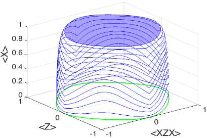
(b)

Figure 3: Convex set for 1D cluster model with system size $N=12$ . (a) represents convex set under OBC while (b) is for PBC. For both cases, the $B_{x}$ field is added only on two boundary sites (one for each boundary). The result is obtained using ED method. $B_{x}=0$ is represented by the green line in both cases. A dramatic difference between the two cases is that a small region reminiscent of ruled surface exists in (a) but is absent in (b).

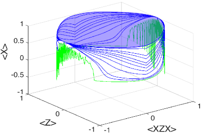
(a)

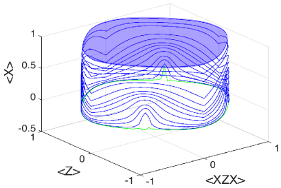
(b)

Figure 4: Convex set for 1D cluster model with system size $N=60$. (a) is for OBC while (b) is for PBC. The green vibrational curve is the ruled surface. We use TEBD method with internal dimension $D=40$. Due to numerical error, we can witness two ruled surface with a large but finite system under OBC.

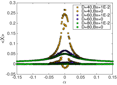
(a)

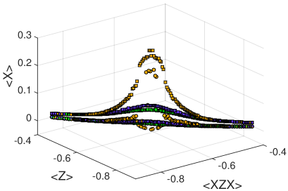
(b)

Figure 5: Finite $D$ scaling for phase transition point under PBC. In both (a) and (b), different colors represent different bond dimension $D$ where yellow, blue and green is for $D=40,60,80$, respectively. Filled square represents $B_{x}=1\times 10^{-2}$ while filled circle represents $B_{x}=0$. With increasing $D$, the small ruled surface in Fig. 4 (b) near phase transition point shrinks. Eventually, this small ruled surface will vanish in the infinite $D$ limit.

In the thermodynamic limit under OBC, when the system is in the SPT phase, the ground state space is spanned by 4 degenerate states. For a large finite system, these four states are nearly degenerate. Thus the state given by TEBD method would be a superposition of these four states because of the limit of the numerical accuracy. This explains the vibrational property of the ruled surface in Fig. 4 (a). As far as we are mainly concerned with the extent of the ruled surface, it is safe to replace the original vibrating curve with its upper hull. Similar vibration was also observed when external magnetic field $B_{x}$ is small enough, e.g. $10^{-4}$, which is not shown in the figure.

A thorough investigation of the numeric errors would be both lengthy and unnecessary. Here we perform a qualitative analysis to show how such errors interestingly lead to the possibility to obtain the ruled surface in a large but finite system, while such a surface should only exist in the thermodynamic limit.

Due the the limit of numerical accuracy, the curve computed for $B_{x}=0$ should be more properly understood as the curve corresponding to $B_{x}=\epsilon$, where $\epsilon$ is a very small number. Denote by $f_{N,B_{x}}$ the curve for a system of size $N$ and the external magnetic field $B_{x}$, or the upper hull of it in case of vibration. Thus our goal is to estimate the difference between $f_{\infty,0}$ (theoretical boundary for the ruled surface in the thermodynamic limit) and $f_{N,\epsilon}$ (curve observed in a finite system with numerical errors). Same as finite system, we can take $f_{\infty,0}\approx f_{\infty,\epsilon}$. Since $f_{\infty,\epsilon}=\lim_{N\to\infty}f_{N,\epsilon}$, for any $\delta>0$, there exists $N(\delta)$, such that $d(f_{\infty,\epsilon},f_{N,\epsilon})<\delta$ for any $N\geq N(\delta)$, where $d$ can be taken, for example, to be the Hausdorff distance between curves. Thus the difference between $f_{\infty,0}\approx f_{\infty,\epsilon}$ and $f_{N,0}\approx f_{N,\epsilon}$ can be arbitrarily small for $N$ large enough. In practice, the convergence is fast such that when $N=60$, the observed ruled surface precisely represents the ruled surface in the thermodynamic limit.

For a large finite system under PBC, there seems to be a small ruled surface at the phase transition point, shown in Fig. 4 (b). With increasing bond dimension $D$, this small area shrinks and eventually vanish in the infinite $D$ limit, shown in Fig. 5. Thus under PBC, there is no ruled surface.

Notice that under both OBC and PBC the upper plane is flat. This is because the normal direction of the corresponding supporting hyperplane is $(0,0,1)$, which corresponds to $J_{1}=J_{2}=0$ for $H_{OBC}$ and $H_{PBC}$. $H_{OBC}$ and $H_{PBC}$ then both become $-B_{x}(X_{1}+X_{N})$, which only acts nontrivially on the boundary, hence are largely degenerate. On the contrary, each line inside the ruled surface (only under OBC) corresponds to a (finite) four-fold degeneracy, which is a non-trivial signal of the SPT order.

V Conclusion and discussion

We study geometry of reduced density matrices for SPT order. Our focus is on the emergence of ruled surface on the boundary of the convex set $\Theta(\{H_{j}\})$. The ground-state degeneracy is a necessary condition for the existence of those ruled surfaces, yet not sufficient.

Compared to the ruled surfaces associated with symmetry-breaking order as discussed in zauner2014symmetry , there is an essential difference for the SPT order. Since there is no local order parameter for SPT order, the ruled surface only exists for the open boundary condition with symmetry-breaking term acting on the boundary. This term is not a thermodynamic variable. Therefore the emergence of ruled surface for SPT order is an effect of geometric locality of the system.

In principle, ruled surface only exists in the thermodynamic limit. However, we have shown that in practice, finite-size calculation suffices to reveal this phenomenon, due to inevitable computational precision uncertainty. This allows us to deal with the calculations using finite systems.

We hope our discussion leads to further understanding of the geometry of reduced density matrices, the effect of geometric locality, and SPT order.

Appendix A Vanishing of ruled surface and nonconvex set

In this Appendix, we explain in detail why we choose the Hamiltonian (17) instead of (12).

If we choose the Hamiltonian (12) and plot the convex set (14), the ruled surface will vanish in the thermodynamic limit. The reason is that the degeneracy of the ground states are owing to the edge states, while the expectation value of the term ${1\over N}{\rm tr}(H_{3}\rho)$ mainly comes from the bulk. If $N\to\infty$, the boundary effect (together with the ruled surface) will disappear due to the normalization factor ${1\over N}$ (See Fig. 6).

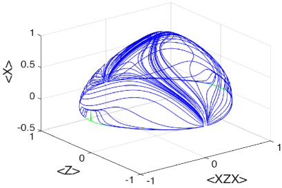
Figure 6: Convex set with a small ruled surface, which is indicated by green lines. The result is obtained by ED method with $N=12$. $\langle XZX\rangle=\frac{1}{N-2}\langle H_{1}^{O}\rangle$, $\langle Z\rangle=\frac{1}{N}\langle H_{2}^{O}\rangle$, $\langle X\rangle=\frac{1}{N}\langle H_{3}\rangle$.

On the other hand, if we plot the set (16) to avoid the vanishing factor $1\over N$, what we obtain is not a convex set (see Fig. 7). This is because we cannot use $\{H_{1}^{O},H_{2}^{O},X_{1}+X_{N}\}$ to construct the Hamiltonian (12).

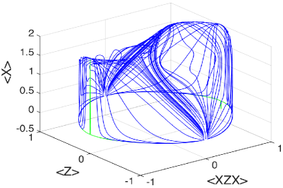
Figure 7: Non-convex set. Result is obtained by ED method with $N=12$. $\langle XZX\rangle=\frac{1}{N-2}\langle H_{1}^{O}\rangle$, $\langle Z\rangle=\frac{1}{N}\langle H_{2}^{O}\rangle$, $\langle X\rangle=\langle X_{1}+X_{N}\rangle$.

References

- [1] A. J. Coleman. Structure of fermion density matrices. Rev. Mod. Phys., 35:668–686, Jul 1963.
- [2] R. M. Erdahl. The convex structure of the set of N-representable reduced 2-matrices. Journal of Mathematical Physics, 13(10):1608–1621, 1972.
- [3] Robert Erdahl and Beiyan Jin. On calculating approximate and exact density matrices. In Jerzy Cioslowski, editor, Many-Electron Densities and Reduced Density Matrices, Mathematical and Computational Chemistry, pages 57–84. Springer US, 2000.
- [4] F. Verstraete and J. I. Cirac. Matrix product states represent ground states faithfully. Phys. Rev. B, 73:094423, Mar 2006.
- [5] Gergely Gidofalvi and David A. Mazziotti. Computation of quantum phase transitions by reduced-density-matrix mechanics. Phys. Rev. A, 74:012501, Jul 2006.
- [6] Christine A. Schwerdtfeger and David A. Mazziotti. Convex-set description of quantum phase transitions in the transverse ising model using reduced-density-matrix theory. The Journal of Chemical Physics, 130(22):–, 2009.
- [7] Alexander A Klyachko. Quantum marginal problem and n-representability. In Journal of Physics: Conference Series, volume 36, page 72. IOP Publishing, 2006.
- [8] Jianxin Chen, Zhengfeng Ji, Chi-Kwong Li, Yiu-Tung Poon, Yi Shen, Nengkun Yu, Bei Zeng, and Duanlu Zhou. Discontinuity of maximum entropy inference and quantum phase transitions. arXiv preprint arXiv:1406.5046, 2014.
- [9] V Zauner, L Vanderstraeten, D Draxler, Y Lee, and F Verstraete. Symmetry breaking and the geometry of reduced density matrices. arXiv preprint arXiv:1412.7642, 2014.
- [10] Josiah Willard Gibbs. Graphical methods in the thermodynamics of fluids. Transcations of the Connecticut Academy, 2:309–342, 1873.
- [11] Josiah Willard Gibbs. A method of geometrical representation of the thermodynamic properties of substances by means of surfaces. Transcations of the Connecticut Academy, 2:382–404, 1873.
- [12] Josiah Willard Gibbs. On the equilibrium of heterogeneous substances. Transcations of the Connecticut Academy, 3:108–248, 1875.
- [13] Robert B. Israel. Convexity in the Theory of Lattice Gases. Princeton University Press, 1979.
- [14] Zheng-Cheng Gu and Xiao-Gang Wen. Tensor-entanglement-filtering renormalization approach and symmetry protected topological order. Phys. Rev. B, 80:155131, 2009.
- [15] C. L. Kane and E. J. Mele. Quantum spin hall effect in graphene. Phys. Rev. Lett., 95:226801, 2005.
- [16] B. Andrei Bernevig and Shou-Cheng Zhang. Quantum spin hall effect. Phys. Rev. Lett., 96:106802, 2006.
- [17] C. L. Kane and E. J. Mele. topological order and the quantum spin hall effect. Phys. Rev. Lett., 95:146802, 2005.
- [18] J. E. Moore and L. Balents. Topological invariants of time-reversal-invariant band structures. Phys. Rev. B, 75:121306, 2007.
- [19] Liang Fu, C. L. Kane, and E. J. Mele. Topological insulators in three dimensions. Phys. Rev. Lett., 98:106803, 2007.
- [20] Xiao-Liang Qi, Taylor Hughes, and Shou-Cheng Zhang. Topological field theory of time-reversal invariant insulators. Phys. Rev. B, 78:195424, 2008.
- [21] F. D. M. Haldane. Nonlinear field theory of large-spin heisenberg antiferromagnets: Semiclassically quantized soliton of the one-dimensional easy-axis neel state. Phys. Rev. Lett., 50:1153, 1983.
- [22] F. D. M. Haldane. Continuum dynamics of the 1-D heisenberg antiferromagnet: Identification with the O(3) nonlinear sigma model. Physics Letters A, 93:464, 1983.
- [23] I. Affleck, T. Kennedy, E. H. Lieb, and H. Tasaki. Valence bond ground states in isotropic quantum antiferromagnets. Commun. Math. Phys., 115:477, 1988.
- [24] Frank Pollmann, Erez Berg, Ari M. Turner, and Masaki Oshikawa. Symmetry protection of topological phases in one-dimensional quantum spin systems. Phys. Rev. B, 85:075125, Feb 2012.
- [25] Xie Chen, Zheng-Cheng Gu, Zheng-Xin Liu, and Xiao-Gang Wen. Symmetry protected topological orders and the group cohomology of their symmetry group. Phys. Rev. B, 87:155114, Apr 2013.
- [26] Xie Chen, Zheng-Cheng Gu, Zheng-Xin Liu, and Xiao-Gang Wen. Symmetry-protected topological orders in interacting bosonic systems. Science, 338(6114):1604–1606, 2012.
- [27] Xie Chen, Zheng-Cheng Gu, and Xiao-Gang Wen. Classification of gapped symmetric phases in one-dimensional spin systems. Phys. Rev. B, 83:035107, Jan 2011.
- [28] Xie Chen, Zheng-Cheng Gu, and Xiao-Gang Wen. Complete classification of one-dimensional gapped quantum phases in interacting spin systems. Phys. Rev. B, 84:235128, Dec 2011.
- [29] N. Schuch, D. Perez-Garcia, and I. Cirac. Classifying quantum phases using matrix product states and projected entangled pair states. Phys. Rev. B, 84:165139, 2011.
- [30] Hans J Briegel and Robert Raussendorf. Persistent entanglement in arrays of interacting particles. Physical Review Letters, 86(5):910, 2001.
- [31] Robert Raussendorf and H. J. Briegel. A one-way quantum computer. Physical Review Letters, 86(22):5188, 2001.
- [32] Dominic V Else, Stephen D Bartlett, and Andrew C Doherty. Symmetry protection of measurement-based quantum computation in ground states. New Journal of Physics, 14(11):113016, 2012.
- [33] Stein Olav Skrovseth and Stephen D Bartlett. Phase transitions and localizable entanglement in cluster-state spin chains with ising couplings and local fields. Physical Review A, 80(2):022316, 2009.
- [34] Andrew C Doherty and Stephen D Bartlett. Identifying phases of quantum many-body systems that are universal for quantum computation. Physical Review Letters, 103(2):020506, 2009.
- [35] Bei Zeng and Duan-Lu Zhou. Topological and error-correcting properties for symmetry-protected topological order. arXiv preprint arXiv:1407.3413, 2014.
- [36] J. H. H. Perk, H. W. Capel, M. J. Zuilhof, and Th. J. Siskens. On a soluble model of an antiferromagnetic chain with alternating interactions and magnetic moments. Physica A, 81:319–348, 1975.
- [37] J. H. H. Perk and H. W. Capel. Time-dependent xx-correlation functions in the one-dimensional xy-model. Physica A, 89:265–303, 1977.
- [38] J. H. H. Perk, H. W. Capel, and Th. J. Siskens. Time-correlation functions and ergodic properties in the alternating xy-chain. Physica A, 89:304–325, 1977.
- [39] J. H. H. Perk and H. Au-Yang. New results for the correlation functions of the ising model and the transverse ising chain. Journal of Statistical Physics, 135:599–619, 2009.
- [40] A. J. Daley, C. Kollath, U. Schollwock, and G. Vidal. Time-dependent density-matrix renormalization-group using adaptive effective hilbert spaces. J. Stat. Mech.: Theor. Exp, 2004:P04005, Apr 2004.
- [41] G. Vidal. Efficient classical simulation of slightly entangled quantum computations. Phys. Rev. Lett, 91:147902, Oct 2003.
- [42] G. Vidal. Efficient simulation of one-dimensional quantum many-body systems. Phys. Rev. Lett, 93:040502, July 2004.