Event-by-event distribution of magnetic field energy over initial fluid energy density in $\sqrt{s_{\rm NN}}$= 200 GeV Au-Au collisions

Abstract

We estimate the event-by-event (e-by-e) distribution of the ratio ($\sigma$) of the magnetic field energy to the fluid energy density in the transverse plane of Au-Au collisions at $\sqrt{s_{\rm NN}}$ = 200 GeV. A Monte-Carlo (MC) Glauber model is used to calculate the $\sigma$ in the transverse plane for impact parameter b=0, 12 fm at time $\tau_{i}\sim$0.5 fm. The fluid energy density is obtained by using Gaussian smoothing with two different smoothing parameter $\sigma_{g}$=0.25 , 0.5 fm. For $b=0~{}\rm fm$ collisions $\sigma$ is found to be $\ll$ 1 in the central region of the fireball and $\sigma\gtrsim$ 1 at the periphery. For b=12 fm collisions $\sigma\gtrsim$ 1. The e-by-e correlation between $\sigma$ and the fluid energy density ($\varepsilon$) is studied. We did not find strong correlation between $\sigma$ and $\varepsilon$ at the centre of the fireball, whereas they are mostly anti-correlated at the periphery of the fireball.

I Introduction

The most strongest known magnetic field (B$\sim 10^{18}-10^{19}$Gauss) in the universe is produced in laboratory experiments of Au-Au or Pb-Pb collisions in the collider experiments at Relativistic Heavy Ion Collider (RHIC) and at Large Hadron Collider (LHC). Previous theoretical studies show that the intensity of the produced magnetic field rises approximately linearly with the centre of mass energy ($\sqrt{s_{{\rm NN}}}$) of the colliding nucleons Bzdak:2011yy ; Deng:2012pc . The Lorentz boosted electric fields in such collisions also becomes very strong which is same order of magnitude as magnetic field ($e\vec{B}\approx e\vec{E}\sim 10m_{\pi}^{2}$ for a typical Au-Au collision at top RHIC energy $\sqrt{s_{\rm NN}}$= 200 GeV), where $m_{\pi}$ is the pion mass. Such intense electric and magnetic fields are strong enough to initiate the particle production from vacuum via Schwinger mechanismKEKIntense:2010 . Using quantum chromodynamics it was shown in Ref. Simonov:2012if that beyond a critical value of magnetic field the quark-antiquark state can possibly attain negative mass (in the limit of large number of colours). Thus it is important to know if there is truly an upper limit of magnetic field intensity allowed by the quantum chromodynamics when applied in heavy ion collisions. Or the magnetic field can grow to arbitrary large value with increasing $\sqrt{s_{\rm NN}}$ as predicted in some earlier studies Bzdak:2011yy ; Deng:2012pc . In this work we shall calculate the electromagnetic field intensity without considering any such constraints, i.e, we assume that the electric and magnetic fields can attain any arbitrary large values.

There are several other interesting recent studies related to the effect of ultra-intense magnetic fields in heavy-ion collisions. Here we briefly mention a few of them which might be relevant to the present study. In presence of a strong magnetic field as created in heavy-ion collisions, a charge current is induced in the Quark Gluon Plasma (QGP), leading to what is known as the “chiral magnetic effect” (CME) Kharzeev:2007jp . Within a 3+1 dimensional anomalous hydrodynamics model a charge dependent hadron azimuthal correlations was found to be sensitive to the CME in Ref. Hirono:2014oda . Along with CME, it was also predicted theoretically that massless fermions with the same charge but different chirality will be separated, yielding what is called the “chiral separation effect” (CSE). A connection between these effects and the Berry phase in condensed matter was also pointed out in Ref. Chen:2012ca ; Stephanov:2012ki ; Son:2012zy . In hadronic phase a significant changes in the hadron multiplicity was observed in presence of a strong magnetic field within a statistical hadron resonance gas model in Ref.  Bhattacharyya:2015pra . There are lot of other important relevant work in this new emerging field which we cannot refer here, one can see recent reviews on this topic in Ref.  Kharzeev:2013ffa ; Bzdak:2012ia ; Kharzeev:2015kna for more details.

The relativistic hydrodynamic models have so far nicely explained the experimentally measured anisotropic particle production in the azimuthal directions in heavy ion collisions. The success of hydrodynamics model shows that a locally equilibrated QGP with small ratio of shear viscosity to entropy density is formed after the collision within a short time interval $\sim$0.2-0.6 fm Shen:2011zc ; Romatschke ; Heinz ; Roy:2012jb ; Heinz:2011kt ; Niemi:2012ry ; Schenke:2011bn . It is also well known that the final momentum anisotropy in hydrodynamic evolution is very sensitive to the initial (geometry) state of the nuclear collisions. So far almost all the hydrodynamic models studies have neglected any influence of magnetic fields on the initial fluid energy-density or on the space-time evolution of QGP. But as we know the initial magnetic field is quite large, it is important to investigate the relative importance of large electro-magnetic field on the usual hydrodynamical evolution of QGP. For that one need a full 3+1 dimensional magnetohydrodynamic code to numerically simulate the space time evolution of QGP with magnetic fields. While one can gain some insight about the relative importance of the magnetic filed on the initial energy density of the QGP fluid by estimating the quantity plasma sigma, which is the dimensionless ratio of magnetic field energy $\frac{B^{2}}{2}$ to the fluid energy density($\varepsilon$) : $\sigma=\frac{B^{2}}{2\varepsilon}$. In plasma $\sigma\sim$1 indicates that one can no longer neglect the effect of magnetic fields in the plasma evolution (in some situation $\sigma\sim$ 0.01 may also effect the hydrodynamic evolution) Lyutikov:2011vc ; Kennel:1983 ; Roy:2015kma ; Spu:2015kma . In the present study we use MC-Glauber model Lin:2004en ; Miller:2007ri to calculate e-by-e magnetic fields and fluid energy density in Au-Au collisions at $\sqrt{s_{\rm NN}}=$ 200 GeV and investigate the relative importance of the magnetic field on initial fluid energy density.

As mentioned earlier, the typical magnetic field produced in a mid-central Au-Au collisions at $\sqrt{s_{\rm NN}}=200\rm GeV$ reaches $\sim 10m_{\pi}^{2}$, which corresponds to field energy density of $\sim 5\,{\rm GeV}/{\rm fm}^{3}$. Hydrodynamical model studies show that the initial energy density for such cases is $\sim 10\,{\rm GeV}/{\rm fm}^{3}$, thus implying $\sigma\sim 0.2$ under these conditions. However, the magnetic field produced at the time of collisions decays very quickly if QGP does not possess finite electrical conductivity Gursoy:2014aka ; Zakharov:2014dia ; Tuchin:2013apa . Thus in order to correctly estimate $\sigma$, one need to consider the proper temporal evolution of magnetic fields until the thermalisation time ($\tau_{i}\sim 0.5fm$ for Au-Au collisions at RHIC) when the hydrodynamic evolution starts. Since the spatial distribution of fluid energy density as well as the electromagnetic fields varies e-by-e we also calculate $\sigma$ accordingly. The spatial distribution of electric and magnetic fields in heavy ion collisions was previously studied in Ref.Zhong:2015dia ; Voronyuk:2011jd .

In present work we study the spatial distribution of $\sigma$ in $\sqrt{s_{\rm NN}}=200$ GeV Au-Au collisions for two different impact parameters (b=0, and 12 fm). The temporal evolution of the magnetic fields after the collision is taken into account in a simplified manner which will be discussed in the next section. We also investigate the correlation between $\sigma$ and fluid energy density in the transverse plane. The paper is organised as follows: in the next section, we discuss about the formalism. Our main result and discussion are presented in section III. A summary is given at the end in section IV.

II Formalism and setup

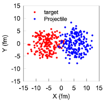
Figure 1: Distribution of nucleons inside target and projectile nuclei in a typical Au-Au collisions at $\sqrt{s_{\rm NN}}$ =200 GeV for b=12 fm.

We constructed a spatial grid of size 10 fm in each direction (X and Y) with the corresponding grid spacing of $\Delta x$ = $\Delta y$ = 0.5 fm for e-by-e calculation of electromagnetic fields and fluid energy density in the plane transverse to the trajectory of the colliding nuclei. The position of colliding nucleons are obtained from MC-Glauber model in e-by-e basis. The position of nucleons are randomly distributed according to the Wood-Saxon nuclear density distribution (as shown in Fig (1)). We adopt the usual convention used in heavy ion collisions for describing the geometry of the nuclear collisions , i.e., the impact parameter vector $(\vec{b})$ of the collision is along X axes and the colliding nuclei are symmetrically situated around the (0,0) point of the computational grid. The electric and magnetic fields at point $\vec{r}(x,y)$ at time $t$ due to all charged protons inside two colliding nucleus are calculated from the Lienard-Weichart formula

$$\vec{E}\left(\vec{r},t\right)=\frac{e}{4\pi}\sum_{i=1}^{{N}_{proton}}{{Z}_{i}\frac{\vec{{R}_{i}}-{R}_{i}\vec{{v}_{i}}}{{\left({R}_{i}-\vec{{R}_{i}}\cdot\vec{{v}_{i}}\right)}^{3}}\left(1-{v}_{i}^{2}\right),}$$ (1)

$$\vec{B}\left(\vec{r},t\right)=\frac{e}{4\pi}\sum_{i=1}^{{N}_{proton}}{{Z}_{i}\frac{\vec{{v}_{i}}\times\vec{{R}_{i}}}{{\left({R}_{i}-\vec{{R}_{i}}\cdot\vec{{v}_{i}}\right)}^{3}}\left(1-{v}_{i}^{2}\right)}.$$ (2)

Where $\vec{E}$ and $\vec{B}$ are the electric and magnetic field vector respectively, e is the charge of an electron, Z is the number of proton inside each nucleus, $\vec{R_{i}}=\vec{x}-\vec{x_{i}}(t)$ is the distance from a charged proton at position $\vec{x_{i}}$ to $\vec{x}$ where the field is evaluated, $\vec{v_{i}}$ is the velocity of the $i$-th proton inside the colliding nucleus. $R_{i}$ is the magnitude of $\vec{R_{i}}$. The summation runs over all proton $(N_{proton})$ inside the two colliding nuclei. Following Ref. Bzdak:2011yy we assume that because of the large Lorentz factor ($\gamma\sim 100$) the colliding nuclei are highly Lorentz contracted along $z$ direction and all the colliding protons have same velocity $v_{i}^{first}=\left(0,0,v_{z}\right)$ and $v_{i}^{second}=\left(0,0,-v_{z}\right)$. $v_{z}$ is related to the c.m energy ($\sqrt{s_{\rm NN}}$) through the relationship ${v}_{z}=\sqrt{1-{\left(\frac{2{m}_{p}}{\sqrt{{s}_{\rm NN}}}\right)}^{2}}$, where $m_{p}$ is the proton mass. Note that according to Eq. (1) and (2) the electric and magnetic fields diverge as ${\vec{R}}_{i}\rightarrow 0$, to remove this singularity we assume a lower value $R_{cut}=$ 0.3 fm as used in Ref Bzdak:2011yy . This particular value of $R_{cut}=$ 0.3 fm was fixed as an effective distance between partons and it was found that the calculated electromagnetic field has weak dependence for $0.3fm\leq{R}_{cut}\leq 0.6fm$. We note that the quantities $e\vec{B}$ and $e\vec{E}$ has dimension $\rm GeV^{2}$ and the conversion from $\rm GeV^{2}$ to Gauss is given by $1\rm GeV^{2}$ = $5.12\times 10^{19}$ Gauss.

It is customary to use Milne co-ordinate ($\tau=\sqrt{\left(t^{2}-z^{2}\right)},x,y,\eta=\frac{1}{2}ln\left(\frac{t+z}{t-z}\right)$) in heavy ion collisions. For our case we shall concentrate on the mid-rapidity region (z$\approx$0) where $t\sim\tau$.

By using the MC-Glauber model we also compute the fluid energy density in transverse plane from the position of wounded nucleons. This is a common practice to initialise energy density for e-by-e hydrodynamics simulations. Since the positions of the wounded nucleons ($N_{\rm wound}$) are like delta function in co-ordinate space, in order to calculate the energy density profile for hydrodynamics simulations one need to smooth the initial profile by introducing Gaussian smearing for every colliding nucleons. The fluid energy density $\varepsilon$ is parameterised as

$$\varepsilon\left(x,y,\sigma_{g},\vec{b}\right)=k\sum_{i=1}^{{N}_{wound}}{{e}^{-\frac{{\left(x-{x}_{i}(\vec{b})\right)}^{2}+{\left(y-{y}_{i}(\vec{b})\right)}^{2}}{2{\sigma_{g}}^{2}}}},$$ (3)

here $x,y$ is the co-ordinate of computational grid, $x_{i}(\vec{b}),y_{i}(\vec{b})$ are the co-ordinate of wounded nucleons for an impact parameter $\vec{b}$, $\sigma_{g}$ is the Gaussian smearing which is taken to be 0.5 fm (unless stated otherwise) for our calculation. $k$ is a constant which is tuned to match the initial central energy density for event averaged case. We estimate $k$=6 which results in the initial central energy density $40GeV/fm^{3}$ for $b=0$ fm collision. This is the typical value of initial energy density used in e-by-e hydrodynamics model to reproduce the experimental measured charged particle multiplicity in Au-Au collisions at $\sqrt{s_{\rm NN}}$=200 GeV for an initial time $\tau_{i}\sim$ 0.5 fm Roy:2012jb . The same $k$ factor is used to calculate the initial energy density for all other impact parameter.

Once we calculate the electromagnetic field and the fluid energy density in the transverse plane, the plasma $\sigma(x,y,\vec{b})=\frac{B^{2}(x,y,\vec{b})}{2\varepsilon(x,y,\vec{b})}$ is readily obtained for each event. For our case we only considered the transverse components $B_{x}$ and $B_{y}$ to calculate the total magnetic energy density, since $B_{z}\ll B_{x},B_{y}$. As mentioned, the hydrodynamics expansion of the QGP fluid starts after a time $\sim$ 0.5 fm, and because of the relativistic velocities of the charged protons the produced magnetic fields decays very quickly. If there is no conducting medium then the magnetic field decay as $\sim t^{-3}$. But in presence of a conducting medium the decay can be substantially delayed Tuchin:2013apa . However, the thermodynamic and transport properties of the nuclear matter right after the collision upto the time when the system reaches local thermal equilibrium is poorly known. Thus we investigate in our study two different scenarios when calculating $\sigma(x,y,\vec{b})$. From now on we will omit $\vec{b}$ in the expression of $\sigma$, and because of spherical symmetry of the colliding nuclei we omit the vector arrow and simply write $b$ for the impact parameter.

(i) In the first scenario, following Ref. Tuchin:2013apa we assume that the matter in pre-equilibrium phase has finite electrical conductivity and the field components are evaluated at $\tau_{i}=$0.5 fm by reducing the magnitudes of the initial magnetic field (at $\tau$=0 fm) to 0.1 times. This is a simplification of the actual scenario, since the time evolution of the fields depend on the electrical conductivity, the impact parameter and on the Lorentz gamma($\gamma$) of the collisions. According to Ref. Tuchin:2013apa the initial electromagnetic field produced in a b=7 fm collision and for an electrical conductivity $\sigma_{el}$=5.8 MeV reduce $\sim$50$\%$ to its original value after $\tau\sim$0.5 fm. Note that for simplification in the numerical simulation we have ignored the impact parameter dependence of the evolution of electromagnetic field in medium as was discussed in Ref. Tuchin:2013apa .

(ii) In the second scenario, we assume the magnetic field is evolved in vacuum (zero electrical conductivity) until the hydrodynamics expansion starts. For this case we reduced the magnitude of the initial electromagnetic field 0.01 times.

We note that in reality the situation may lie in between the above mentioned two scenarios. From now on we denote the first and second scenario by medium and vacuum respectively.

We consider 1000 nucleus-nucleus collisions for our present calculation for each impact parameter.

III Results and discussion

At first we shall concentrate on the electromagnetic fields computed at the centre of the fireball (i.e. at point $\rm x=y=0$ in our computational grid). Fig. 2 shows the event averaged value of magnetic and electric fields as a function of impact parameter $b$. The $B_{y}$ , its absolute value $|B_{y}|$, and $x$ component of the electric field $E_{x}$ are shown by pink dashed, blue dotted, and black solid lines respectively. We note that our result is consistent with the result of Ref. Bzdak:2011yy . We also checked other components of electric and magnetic fields and they are found to be consistent with Ref. Bzdak:2011yy .

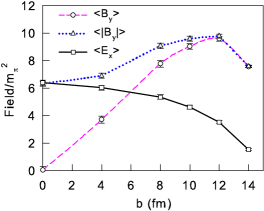
Figure 2: Impact parameter dependence of event averaged magnetic and electric fields at the centre of the fireball for Au-Au collisions at $\sqrt{s_{\rm NN}}$=200 GeV.

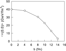
Figure 3: Impact parameter dependence of event averaged central energy density ($<\varepsilon\left(0,0\right)>$) of fluid for Au-Au collisions at $\sqrt{s_{\rm NN}}$ =200 GeV.

The electric and magnetic fields are created in high energy heavy-ion collisions in presence of the electrically charged protons inside the two colliding nucleus. Whereas both neutron and protons inside the colliding nuclei deposit energy in the collision zone as a result of elastic and inelastic collisions among them. Since the positions of protons in the colliding nucleus is different with that of the positions of all nucleons, resulting spatial distribution of the electromagnetic field is expected to differ from that of the initial fluid energy density. Fig. 3 shows the event averaged value of fluid energy density at point ($\rm x=y=0$) as a function of impact parameter $b$. The energy density is obtained from Eq. 3 for $k=$6. This specific value of $k$ was chosen in order to obtain the central energy density $\sim$ 40 $\rm GeV/fm^{3}$ for $b=0$ fm collisions. From previous studies Roy:2012jb we note that the initial central energy density for central ($0-5\%$ centrality which corresponds to $b\sim$ 2 fm) Au-Au collisions requires $\varepsilon\sim 40~{}\rm GeV/fm^{3}$ at initial time $\tau_{i}=0.6~{}\rm fm$ at the centre of the fireball ($\rm x=y=0$) to reproduce the experimentally measured charged hadron multiplicity at $\sqrt{s_{\rm NN}}=200\rm GeV$. However, we note that a different initial time ($\tau_{i}$) will give different initial energy density Shen:2010uy , in that case the magnitude of magnetic field at $\tau_{i}$ will also be different. From Fig. 2 and Fig. 3 we notice that fluid energy density decreases whereas the intensity of magnetic field increases with $b$. It is thus expected that $\sigma(x,y,b)$ will reach its maximum value for $b\sim$ 12 fm. So far we have shown the event average $\vec{E}(x,y),\vec{B}(x,y)$ and $\varepsilon\left(x,y\right)$ at the center of the collision zone.

Top panel of Fig. 4 shows the event averaged $\varepsilon(x,y)$ for $\rm b=$0 fm collisions. Since the Au nucleus is almost spherical in shape, a head on Au-Au collision deposits energy in an almost circular zone. Different colour schemes in the legend denotes the energy density in unit of $\rm GeV/fm^{3}$. Middle and bottom panel of Fig. 4 shows the corresponding magnetic field energy density $\frac{B^{2}}{2}$ due to the $y$ and $x$ component of $\vec{B}$ respectively, where $\vec{B}$ is calculated at time $\tau=0$. We observe that the distribution of magnetic field energy is similar to the fluid energy density obtained from elastic and inelastic nucleon-nucleon collisions in MC-Glauber model. The magnetic field energy density due to $B_{x}$ and $B_{y}$ is peaked at the centre and has a SO(2) rotational symmetry for $\rm b$=0 fm collision. This is not surprising since the positions of the protons for $\rm b=$0 fm collisions have such rotational symmetry about the centre of the fireball in the transverse plane for event averaged case. The situation for a non-zero impact parameter collisions becomes different . The overlap zone between the two nuclei becomes elliptical, as can be seen from the top panel of Fig. 5 which corresponds to $\varepsilon(x,y)$ for $\rm b=$12 fm. The middle and bottom panel of Fig. 5 shows the corresponding energy density for $B_{y}$ and $B_{x}$ components. We find that the field energy density due to $B_{y}$ has similar shape as fluid energy density, but that due to $B_{x}$ has maximum in a dumbbell shaped region which is different from the initial fluid energy density.

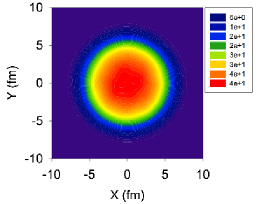
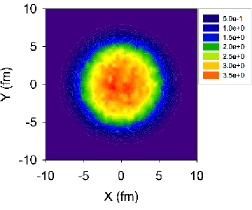
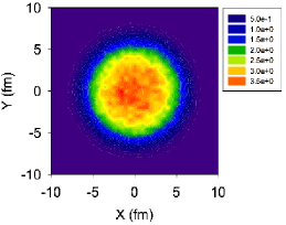
Figure 4: Top Panel: 1000 event averaged initial energy density of QGP for b=12 fm Au-Au collisions at $\sqrt{s_{\rm NN}}$=200 GeV. Middle Panel: 1000 event averaged magnetic field energy density calculated from y component of the magnetic field for b=12 fm Au-Au collisions at $\sqrt{s_{\rm NN}}$ GeV. Bottom Panel: Same as middle panel but for the $x$ component of the magnetic fields $B_{x}$.

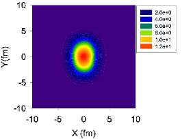
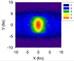
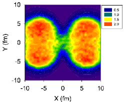
Figure 5: Top Panel: 1000 event averaged initial energy density of QGP for Au-Au at $\sqrt{s_{\rm NN}}$ =200 GeV for impact parameter b=12 fm collisions. Middle Panel: event averaged magnetic field energy density calculated from y component of the magnetic field for b=12 fm Au-Au collisions at $\sqrt{s_{\rm NN}}$ GeV. Bottom Panel: Same as middle panel but for the $x$ component of the magnetic fields $B_{x}$.

So far we have shown event averaged value of $\varepsilon$ and components of $\vec{B}$. It is not clear from the above discussion whether the magnetic field energy density is negligible compared to the initial fluid energy density for every events because both $\varepsilon$ and $\frac{B^{2}}{2}$ are lumpy in the transverse plane as shown in Fig.  6. This leads us to study $\sigma(x,y)$ on e-by-e basis.

III.1 Event-by-event $\sigma(x,y)$

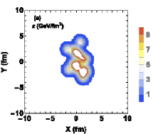
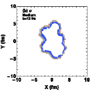
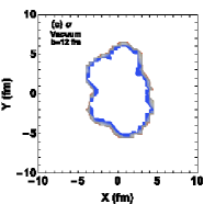
Figure 6: Top panel: fluid energy density , Middle panel: $\sigma\left(x,y\right)$ for the medium , Bottom panel: $\sigma\left(x,y\right)$ for the vacuum in a single b=12 fm Au-Au $\sqrt{s_{\rm NN}}$=200 GeV collision. The shaded annular region in middle and bottom panel corresponds to $0.01\leq\sigma\left(x,y\right)\leq 10$ .

Top panel of Fig. 6 shows the energy density, middle and bottom panels show corresponding $\sigma\left(x,y\right)$ at $\tau=$0.5 fm for evolution of the magnetic field in medium and in vacuum respectively for a single event of b=12 fm collisions. The shaded band in the middle and bottom panels correspond to the zones where $0.01\leq\sigma\left(x,y\right)\leq 10$ (increasing in the outward direction). As expected $\sigma\left(x,y\right)$ reaches its maximum value in regions where $\varepsilon\left(x,y\right)$ becomes small. However, note that those regions of large $\sigma\left(x,y\right)$ strongly depends on the temporal evolution of the magnetic field from $\tau=0\rm fm$ until the hydrodynamics expansion starts at time $\tau_{i}$. This can be seen from the bottom panel of the same figure where the regions of large $\sigma\left(x,y\right)$ moves outward as the magnetic filed for this case decays faster than the case of medium with finite electrical conductivity.

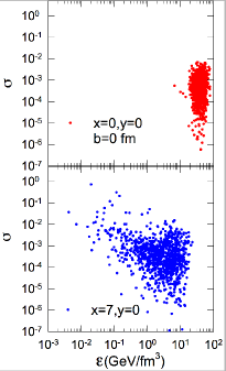
Figure 7: Top panel: e-by-e distribution of $\sigma\left(0,0\right)$ as a function of $\varepsilon\left(0,0\right)$ for b=0 fm Au-Au collisions at $\sqrt{s_{\rm NN}}$ =200 GeV. Bottom panel: same as top panel but for $(\rm x=7,y=0)$.

We observe here that even if the magnetic field decays quickly (as in vacuum) until the hydrodynamics expansion starts, there is a corona of large $\sigma\left(x,y\right)$. It is then important to consider magnetohydrodynamics framework to investigate further the possible effects of those large $\sigma\left(x,y\right)$ zone on the space-time evolution of the QGP fluid.We expect that since the region of large $\sigma$ seems to lie mostly outside the places where $\varepsilon\left(x,y\right)$ is high there will be minor modification in the transverse evolution of the QGP fluid when the effect of magnetic field is taken into account. The above conclusion is made by investigating only one particular event, in order to understand the ensemble of events let us look at the e-by-e distribution of $\sigma\left(x,y\right)$ at the centre ($\rm x=y=0)$ and at the periphery of the collision zone.

Top panel of Fig. 7 shows the e-by-e distribution of $\sigma\left(0,0\right)$ as a function of $\varepsilon\left(0,0\right)$ for b=0 fm collisions. The bottom panel of the same figure shows the event distribution of $\sigma\left(7,0\right)$ versus $\varepsilon\left(7,0\right)$. All results are obtained for magnetic field evolution in medium. Naively one expects that $\sigma\left(x,y\right)$ and $\varepsilon\left(x,y\right)$ should be anti-correlated, i.e., for places where $\varepsilon$ is large $\sigma$ will be small and vice-versa, the same conclusion was made in Ref. Voronyuk:2011jd . But it is clear from Fig. 7 that there is no such simple relationship between $\varepsilon$ and $\sigma$ for b=0 fm collisions in MC-Glauber model . In fact, we notice that at the center of the collision zone $\varepsilon$ and $\sigma$ are almost uncorrelated. For regions at the periphery of the collision zone (bottom panel) we observe similar behaviour, but notice that here $\sigma\left(7,0\right)$ may reach $\sim$ 1 in some events, whereas for $x=y=0$ it never exceed 0.01.

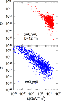
Figure 8: Top panel: e-by-e distribution of $\sigma\left(0,0\right)$ as a function of $\varepsilon\left(0,0\right)$ for b=12 fm Au-Au collisions at $\sqrt{s_{\rm NN}}$ =200 GeV. Bottom panel: same as top panel but for $(\rm x=3,y=0)$.

Now let us discuss the result for $\rm b$=12 fm collisions where the relative importance of magnetic field is expected to be highest. Top panel of Fig. 8 shows the e-by-e distribution of $\sigma\left(0,0\right)$ as a function of $\varepsilon\left(0,0\right)$ for $\rm b$=12 fm collisions. We notice that like $\sigma\left(0,0\right)$ distribution for b=0 fm collisions, most of the events have $\sigma\left(0,0\right)\lesssim$ 0.01. However, for few events $\sigma\left(0,0\right)\sim$ 1. Like $\rm b=0fm$ collisions here we also notice no clear correlation between $\epsilon$ and $\sigma$. The bottom panel of Fig. (8) shows the distribution of $\sigma\left(3,0\right)$ as a function of $\varepsilon\left(3,0\right)$. We notice that a considerable number of events have $\sigma\sim$ 1 for this case.

Next we discuss the event averaged transverse profile of $\sigma\left(x,y\right)$ for $\rm b$=0 and 12 fm as depicted in Fig. 9 and 10 respectively. As expected, the event averaged $\sigma\left(x,y\right)$ in the range $0.01\leq\sigma\leq 10$ for b=0 fm collisions (Fig. 9) form an annular region enclosing the high energy density zone of the QGP fluid. Top panel of Fig.(9) shows the result for magnetic field evolution in vacuum and the bottom panel shows in medium. However, $\sigma\left(x,y\right)$ for b=12 fm collisions shows different spatial distribution as depicted in Fig. 10. The non-trivial contour in this case results from the fact that for some events $\sigma\left(x,y\right)$ becomes very large and the event averaged value is dominated by those large $\sigma$. The top and bottom panel shows the result for vacuum and medium respectively.

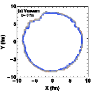
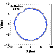
Figure 9: Event averaged $\sigma\left(x,y\right)$ in the range $0.01\leq\sigma\leq 10$ (shaded region) for Au-Au collisions of b=0 fm at $\sqrt{s_{\rm NN}}$ = 200 GeV . Top panel: for vacuum. Bottom panel: for medium.

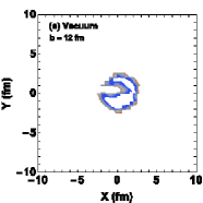
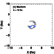
Figure 10: Event averaged $\sigma\left(x,y\right)$ in the range $0.01\leq\sigma\leq 10$ (shaded region) for Au-Au collisions of b=12 fm at $\sqrt{s_{\rm NN}}$ = 200 GeV. Top panel: for vacuum. Bottom panel: for medium.

III.2 Sensitivity of $\sigma(x,y)$ on Gaussian smearing

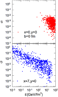
Figure 11: Top panel: e-by-e distribution of $\sigma\left(0,0\right)$ as a function of $\varepsilon\left(0,0\right)$ for Au-Au b=0 fm collisions at $\sqrt{s_{\rm NN}}$ =200 GeV. Bottom panel: same as top panel but for $(x=7,y=0)$. $\sigma_{g}$=0.25 for both the cases.

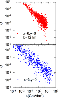
Figure 12: Top panel: e-by-e distribution of $\sigma\left(0,0\right)$ as a function of $\varepsilon\left(0,0\right)$ for Au-Au b=12 fm collisions at $\sqrt{s_{\rm NN}}$ =200 GeV. Bottom panel: same as top panel but for $(x=3,y=0)$. $\sigma_{g}$=0.25 for both the cases.

The Gaussian smearing $\sigma_{g}$ in Eq. (3) is a free parameter which is usually taken in the range $\sim$ 0.1-1.0 fm. Here we discuss the sensitivity of our result on Gaussian smearing by setting $\sigma_{g}=\rm 0.25fm$ which is taken from a recent study Chaudhuri:2015twa . Reducing $\sigma_{g}$ results in much lumpy initial energy density hence we expect a different spatial dependence of $\sigma(x,y)$ compared to the previous case where $\sigma_{g}=0.5\rm fm$ is used. For $\sigma_{g}=0.25\rm fm$ we adjusted $k$ to a new value $k$=17 to keep the event-averaged initial central energy density for b=0 fm collisions same as before i.e., $\sim 40\rm GeV/fm^{3}$ . Top panel of Fig. 11 shows the e-by-e distribution of $\sigma\left(0,0\right)$ as a function of $\varepsilon\left(0,0\right)$ for b=0 fm Au-Au collisions. Bottom panel shows the same but for $\rm x=7,y=0$. Comparing Fig. 7 and 11 we found that changing $\sigma_{g}$ from 0.5 fm to 0.25 fm changes the e-by-e distribution of $\sigma$ vs $\varepsilon$. Since the energy density is more lumpy for $\sigma_{g}=$ 0.25 fm than 0.5 fm, the number of events with large $\sigma$ increases. To see the effect of changed $\sigma_{g}$ in peripheral collisions, we show the e-by-e distribution of $\sigma$ vs $\varepsilon$ for b=12 fm in Fig. 12. Top panel of Fig. 12 shows the e-by-e distribution of $\sigma\left(0,0\right)$ vs $\varepsilon\left(0,0\right)$ and the bottom panel shows e-by-e distribution of $\sigma\left(3,0\right)$ vs $\varepsilon\left(3,0\right)$. It is clear that for b=12 fm collisions the correlation between $\sigma$ and $\varepsilon$ at the center ($x=y=0$) is sensitive to $\sigma_{g}$, and the maximum value of $\sigma\sim$ 1, in contrary to what was observed for the case b=0 fm collisions.

IV Summary

We have studied the relative importance of magnetic field energy on initial fluid energy density of the QGP by evaluating $\sigma=\frac{B^{2}}{2\varepsilon}$ for Au-Au collisions at $\sqrt{s_{\rm NN}}$= 200 GeV. The fluid energy density and electromagnetic fields are computed by using MC-Glauber model. The electromagnetic field and initial fluid energy density are calculated by using following parameters: the cutoff distance $R_{cut}=0.3\rm fm$, Gaussian smearing parameter $\sigma_{g}=$0.5, (and 0.25 fm) and the scalar multiplicative factor $k=$6, (and 17). The initial energy density (at time $\tau_{i}=$ 0.5 fm) for the fluid is fixed to $\sim$ 40 $\rm GeV/fm^{3}$. The ratio of the magnetic field energy density to the fluid energy density $\sigma$ is evaluated in the transverse plane for two different impact parameters $\rm b=$0 , and 12 fm. We find that for most of the events, at the centre of the collision zone $\sigma\left(0,0\right)$ $\ll$ 1 for both b=0, and 12 fm collisions. However, at the periphery of the collision zone where $\varepsilon$ becomes small we observed a region of large $\sigma$. For large impact parameter collisions $\sigma$ becomes larger for peripheral collisions (large $b$) compared to central (small $b$) collisions as a result of increase in magnetic field and decrease in fluid energy density. We observe that in central collisions (b= 0 fm) at the center of collision zone $\sigma\ll$1 for most of the events. However, large $\sigma$ is observed in the outer regions of collision zone. In peripheral collisions $\sigma$ becomes quite large at both center and periphery of the collision zone. From this observation we conclude that initial strong magnetic field might contribute to the total initial energy density of the Au-Au collisions (or other similar heavy ion collisions like Pb-Pb) significantly. However, the true effect of large $\sigma$ (or large magnetic fields) will remain unclear unless one performs realistic magneto-hydrodynamics simulation with the proper initial conditions, for example see Ref. Lyutikov:2011vc ; Kennel:1983 ; Roy:2015kma ; Spu:2015kma for some theoretical estimates. Note that the result in this paper are obtained for a specific model of initial conditions (MC-Glauber model) with few free parameters. We have not explored all possible allowed values of these free parameters. In future we may incorporate other initial conditions and more realistic time evolution of the electromagnetic fields in the pre-equilibrium phase (as described in Ref. Tuchin:2013apa ) to study the effect of magnetic fields on initial fluid energy density distribution. It is also interesting to study the similar thing for lower $\sqrt{s_{\rm NN}}$ collisions where the decay of magnetic field in vacuum is supposed to be much slower than the present case because of the slower speed of colliding nuclei, and also the corresponding initial energy density for such cases is smaller than the present case of Au-Au collisions at $\sqrt{s_{\rm NN}}=200\rm GeV$.

Acknowledgment: VR and SP are supported by the Alexander von Humboldt Foundation. Authors would like to thank Dirk Rischke for discussion.

References

- (1) A. Bzdak and V. Skokov, Phys. Lett. B 710, 171 (2012) [arXiv:1111.1949 [hep-ph]].
- (2) W. T. Deng and X. G. Huang, Phys. Rev. C 85, 044907 (2012) [arXiv:1201.5108 [nucl-th]].
- (3) KEK. Proceedings of the international Conference on Physics in Intense Fields (PIF 2010), November 24-26, 2010 Tsukuba, Japan. Editor: K. Itakura, S. Iso and T. Takahashi , http://atfweb.kek.jp/pif2010/
- (4) Y. A. Simonov, B. O. Kerbikov and M. A. Andreichikov, arXiv:1210.0227 [hep-ph].
- (5) D. E. Kharzeev, L. D. McLerran and H. J. Warringa, Nucl. Phys. A 803, 227 (2008) [arXiv:0711.0950 [hep-ph]].
- (6) Y. Hirono, T. Hirano and D. E. Kharzeev, Phys. Rev. C 91, 054915 (2015) [arXiv:1412.0311 [hep-ph]].
- (7) J. W. Chen, S. Pu, Q. Wang and X. N. Wang, Phys. Rev. Lett. 110, no. 26, 262301 (2013) [arXiv:1210.8312 [hep-th]].
- (8) M. A. Stephanov and Y. Yin, Phys. Rev. Lett. 109, 162001 (2012) [arXiv:1207.0747 [hep-th]].
- (9) D. T. Son and N. Yamamoto, Phys. Rev. D 87, no. 8, 085016 (2013) [arXiv:1210.8158 [hep-th]].
- (10) D. E. Kharzeev, Prog. Part. Nucl. Phys. 75, 133 (2014) [arXiv:1312.3348 [hep-ph]].
- (11) A. Bzdak, V. Koch and J. Liao, Lect. Notes Phys. 871, 503 (2013) [arXiv:1207.7327].
- (12) D. E. Kharzeev, arXiv:1501.01336 [hep-ph].
- (13) C. Shen, S. A. Bass, T. Hirano, P. Huovinen, Z. Qiu, H. Song and U. Heinz, J. Phys. G 38, 124045 (2011) [arXiv:1106.6350 [nucl-th]].
- (14) P. Romatschke and U. Romatschke, Phys. Rev. Lett. 99, 172301 (2007); M. Luzum and P. Romatschke, Phys. Rev. C 78, 034915 (2008).
- (15) H. Song and U. W. Heinz, Phys. Lett. B 658, 279 (2008); Phys. Rev. C 78, 024902 (2008).
- (16) V. Roy, A. K. Chaudhuri and B. Mohanty, Phys. Rev. C 86, 014902 (2012) [arXiv:1204.2347 [nucl-th]].
- (17) H. Niemi, G. S. Denicol, P. Huovinen, E. Molnar and D. H. Rischke, Phys. Rev. C 86, 014909 (2012) [arXiv:1203.2452 [nucl-th]].
- (18) U. Heinz, C. Shen and H. Song, AIP Conf. Proc. 1441, 766 (2012) [arXiv:1108.5323 [nucl-th]].
- (19) B. Schenke, S. Jeon and C. Gale, Phys. Rev. C 85, 024901 (2012) [arXiv:1109.6289 [hep-ph]].
- (20) A. Bhattacharyya, S. K. Ghosh, R. Ray and S. Samanta, arXiv:1504.04533 [hep-ph].
- (21) M. Lyutikov and S. Hadden, Phys. Rev. E 85, 026401 (2012) [arXiv:1112.0249 [astro-ph.HE]].
- (22) C. F. Kennel and F. V. Hadden, The. Astrophysical . Journal, 283, 694-709 (1984)
- (23) V. Roy, S. Pu, L. Rezzolla and D. Rischke, arXiv:1506.06620 [nucl-th].
- (24) S. Pu, V. Roy, L. Rezzolla and D. Rischke, in preparation.
- (25) Z. W. Lin, C. M. Ko, B. A. Li, B. Zhang and S. Pal, Phys. Rev. C 72, 064901 (2005) [nucl-th/0411110].
- (26) M. L. Miller, K. Reygers, S. J. Sanders and P. Steinberg, Ann. Rev. Nucl. Part. Sci. 57, 205 (2007) [nucl-ex/0701025].
- (27) U. Gursoy, D. Kharzeev and K. Rajagopal, Phys. Rev. C 89, no. 5, 054905 (2014) [arXiv:1401.3805 [hep-ph]].
- (28) B. G. Zakharov, Phys. Lett. B 737, 262 (2014) [arXiv:1404.5047 [hep-ph]].
- (29) K. Tuchin, Phys. Rev. C 88, no. 2, 024911 (2013) [arXiv:1305.5806 [hep-ph]].
- (30) Y. Zhong, C. B. Yang, X. Cai and S. Q. Feng, arXiv:1507.07743 [hep-ph].
- (31) V. Voronyuk, V. D. Toneev, W. Cassing, E. L. Bratkovskaya, V. P. Konchakovski and S. A. Voloshin, Phys. Rev. C 83, 054911 (2011) [arXiv:1103.4239 [nucl-th]].
- (32) C. Shen, U. Heinz, P. Huovinen and H. Song, Phys. Rev. C 82, 054904 (2010) [arXiv:1010.1856 [nucl-th]].
- (33) A. K. Chaudhuri, arXiv:1507.04898 [nucl-th].