New Signatures of the Milky Way Formation in the Local Halo and Inner Halo Streamers in the Era of Gaia

Abstract

We explore the vicinity of the Milky Way through the use of spectro-photometric data from the Sloan Digital Sky Survey and high-quality proper motions derived from multi-epoch positions extracted from the Guide Star Catalogue II database. In order to identify and characterise streams as relics of the Milky Way formation, we start with classifying, select, and study $2417$ subdwarfs with $\rm{[Fe/H]<-1.5}$ up to $3$ kpc away from the Sun as tracers of the local halo system. Then, through phase-space analysis, we find statistical evidence of five discrete kinematic overdensities among $67$ of the fastest-moving stars, and compare them to high-resolution N-body simulations of the interaction between a Milky-Way like galaxy and orbiting dwarf galaxies with four representative cases of merging histories.
The observed overdensities can be interpreted as fossil substructures consisting of streamers torn from their progenitors; such progenitors appear to be satellites on prograde and retrograde orbits on different inclinations. In particular, of the five detected overdensities, two appear to be associated, yelding twenty-one additional main-sequence members, with the stream of Helmi et al. (1999) that our analysis confirms on a high inclination prograde orbit. The three newly identified kinematic groups could be associated with the retrograde streams detected by Dinescu (2002) and Kepley et al. (2007); whatever their origin, the progenitor(s) would be on retrograde orbit(s) and inclination(s) within the range $10^{\circ}\div 60^{\circ}$.
Finally, we use our simulations to investigate the impact of observational errors and compare the current picture to the promising prospect of highly improved data expected from the Gaia mission.

1. Introduction

The formation and evolution of galaxies is one of the outstanding problems in astrophysics, one which can be profitably engaged directly through detailed study of our own Galaxy, the Milky Way (e.g., Freeman & Bland-Hawthorn, 2002; Helmi, 2008).

In the context of hierarchical structure formation, galaxies such as the Milky Way grow by mergers and accretion of smaller systems, perhaps similar to what are now observed as dwarf galaxies. These satellite galaxies – torn apart by the tidal gravitational field of the parent galaxy – are progressively disrupted, giving rise to trails of stellar debris streams along their orbits, spatial signatures that eventually disappear due to dynamical mixing. After the accretion era ends, a spheroidal halo-like component is left from their collective assembly (e.g., Searle & Zinn, 1978; Bullock & Johnston, 2005; Abadi et al., 2006; Moore et al., 2006; Sales et al., 2007; De Lucia, 2012).

Of all the Galactic components, it is indeed the stellar halo that offers the best opportunity for probing details of the merging history of the Milky Way (see, e.g., Helmi, 2008). Past explorations have demonstrated that there is a concrete possibility to identify groups of halo stars that originate from common progenitor satellites (Eggen, 1977; Ibata et al., 1994; Majewski et al., 1996; Helmi et al., 1999; Chiba & Beers, 2000; Dinescu, 2002; Ibata et al., 2003; Kepley et al., 2007; Klement et al., 2009; Morrison et al., 2009; Schlaufman et al., 2009; Smith et al., 2009; Duffau et al., 2014).

Simulations show that a Milky-Way mass galaxy within a $\rm{\Lambda}$CDM universe will have halo stars associated with substructures and streams (e.g., Johnston, 1998; Harding et al., 2001; Starkenburg et al., 2009; Helmi et al., 2011; Gomez et al., 2013). These substructures, much like those seen in the halo system of the Milky Way, are sensitive to recent (within the last $8$ Gyr) merging events, and are more prominent in the outer region of the halo (galactocentric radii beyond $15-20$ kpc), whereas the inner-halo region appears significantly smoother.

Based on data from the SEGUE spectroscopic survey, Schlaufman et al. (2009) found that metal-poor main-sequence turnoff stars in the inner-halo region of the Milky Way (within $\sim 20$ kpc from the Sun) exhibit clear evidence for radial velocity clustering on small spatial scales (they refer to these as ECHOS, for Elements of Cold HalO Substructure). They estimated that about $10\%$ of the inner-halo turnoff stars belong to ECHOS, and inferred the existence of about $1000$ ECHOS in the entire inner halo volume. Schlaufman et al. (2011) suggest that the most likely progenitors of ECHOS are dwarf spheroidal galaxies with masses on the order of $10^{9}$ M_☉.

In the Solar Neighbourhood, up to $1-2$ kpc of the Sun, stellar streams have also been discovered as overdensities in the phase-space distribution of stars, integrals of motion and action-angle variables (see Klement, 2010, for a review). Prominent examples are the two stellar debris streams in the halo population passing close to the Sun detected by Helmi et al. (1999) when combining high-quality HIPPARCOS proper motions with ground-based observations. Formed via destruction of a satellite whose debris now occupy the inner halo region with no apparent spatial structure, these streamers retain very similar velocities and are seen as clumps in angular momentum space where stars from a common progenitor appear rather confined (Helmi & de Zeeuw, 2000).

Besides the Helmi stream, $\omega$ Centauri (Dinescu, 2002; Majewski et al., 2012), the Kapteyn and Arcturus (e.g., Eggen, 1971) streams, Klement (2010) lists a few other halo substructures found in the solar neighborhood: these are still small numbers compared to the few hundred streams expected (i.e. $300$-$500$, Helmi & White, 1999; Gould, 2003). Actually, recovering fossil structures in the inner halo is considerably more difficult, as strong phase-mixing takes place. This degeneracy can only be broken with 6D (phase-space) or 7D (including abundances) information achievable by integrating astrometry, photometry, and spectroscopy.

The SDSS - GSC II Kinematic Survey (from now on SGKS) we exploit here was produced to serve this task (see Spagna et al., 2010b). In the future, new ground- and space-based surveys such as Gaia (e.g., Perryman et al., 2001; Turon et al., 2005), Gaia ESO Survey (GES; Gilmore et al., 2012), and LAMOST (Zhao et al., 2012) will provide high-precision data that will usher us in a new era of Milky Way studies.

In Sect. 2, we introduce the data used to isolate a sample of nearby halo subdwarfs from the SGKS catalogue. The kinematic and orbital properties of the local halo subdwarf population are discussed in Sect. 3, where we present algorithms to search for kinematic substructures, recovering known streams (Helmi et al., 1999; Dinescu, 2002; Kepley et al., 2007), as well as new kinematic overdensities. In Sect. 4, we present the high-resolution N-body numerical simulations of four minor mergers used to study galaxy interactions and the properties of accretion events in the vicinity of the Sun. In Sect. 5 we investigate the impact of observational errors resulting from current ground-based data and from high accurate data expected from the Gaia satellite. Finally, in Sect. 6, we compare observations to these numerical simulations and infer the nature of the detected fast moving groups.

Table 1 Halo velocity parameters.

$\langle U\rangle$	$\langle V+220\rangle$	$\langle W\rangle$	$\sigma_{U}$	$\sigma_{V}$	$\sigma_{W}$	$\rho_{UV}$	$\rho_{UW}$	$\rho_{VW}$
$\rm{(km~{}s^{-1})}$	$\rm{(km~{}s^{-1})}$	$\rm{(km~{}s^{-1})}$	$\rm{(km~{}s^{-1})}$	$\rm{(km~{}s^{-1})}$	$\rm{(km~{}s^{-1})}$
$15\pm 2$	$25\pm 2$	$-4\pm 2$	$126\pm 1$	$100\pm 1$	$91\pm 1$	$-0.09\pm 0.02$	$-0.18\pm 0.02$	$0.05\pm 0.02$

Note. — The Milky Way halo velocity parameters as determined from our selected sample of 2417 FGK subdwarfs. The table lists mean velocities, dispersions, and corresponding correlation coefficients in Galactic coordinates. Noticeable is the correlation between $U$ and $W$ (see text).

2. The SDSS - GSC II Kinematic Survey (SGKS)

This study is based on a new kinematic catalogue, derived by assembling spectro-photometric stellar data from the Seventh Data Release of the Sloan Digital Sky Survey (SDSS DR7; Abazajian et al., 2009), which included data from the Sloan Extension for Galactic Understanding and Exploration (SEGUE; Yanny et al., 2009), supplemented by astrometric parameters extracted from the database used for the construction of the Second Guide Star Catalogue (GSC II; Lasker et al., 2008). This SDSS - GSC II catalogue contains positions, proper motions, classification, and $ugriz$ photometry for $77$ million sources down to $r\sim 20$, over $9000$ square degrees.

Proper motions are computed by combining multi-epoch positions from SDSS DR7 and the GSC II database; typically, $5-10$ observations are available for each source, spanning up to $50$ years. The typical formal errors on those proper motions are in the range $2-3~{}{\rm mas~{}yr^{-1}}$ per coordinate for $16<r<18.5$, comparable with the internal precision of the SDSS proper motions computed by Munn et al. (2008). Although much of the photographic material (Schmidt plates) used to derive first epoch information is in common with Munn et al. (2008), plate digitisation and measurement processes, and the calibration methods that led to the first epoch positions were somewhat different, with the Munn et al.’ data coming from the USNO-B project. Of particular relevance is the minimisation of systematic errors that can affect proper motion accuracy, a true driver in analysis like those conducted in this study. An accurate validation of our proper motions was discussed in Spagna et al. (2010a).

Radial velocities and astrophysical parameters are available for about $151\,000$ sources cross-matched with the SDSS spectroscopic catalogue Typical accuracy are of $5-10~{}{\rm km~{}s^{-1}}$ in line of sight velocity, $250$ K in effective temperature, ${\rm T_{eff}}$, $0.25$ dex in surface gravity, $\log~{}g$, and $0.20$ dex in metallicity, ${\rm[Fe/H]}$, as estimated within the SEGUE Spectral Parameter Pipeline (SSPP; i. e., Re Fiorentin et al., 2007; Lee et al., 2008a, b; Allende Prieto et al., 2008). We specify that the sample includes only objects with no problems related to the spectrum, and classified without any cautionary flag by the SSPP. In case of multiple spectra, we take the spectrum with the highest signal-to-noise ratio.

From the SDSS - GSC II catalogue, we select as tracers sources with $4500~{}{\rm K}<{\rm T_{eff}}<7500$ K and $\log~{}g>3.5$, corresponding to FGK dwarfs.

The observed magnitudes are corrected for interstellar absorption via the extinction maps of Schlegel et al. (1998) based on the $6.1^{\prime}$ resolution COBE/DIRBE dust map, that we preferred to the more recent, but of inferior resolution ($7^{\prime}$-$14^{\prime}$), reddening maps published by Schlafly et al. (2014). Then, we transformed the $E(B-V)$ to the SDSS photometric system by adopting the extinction ratio $A_{r}/A_{V}=0.875$ (from Table 1 of Girardi et al., 2004), that is appropriate for our FGK dwarf sample.

Photometric distances good to $\sigma_{d}/d\sim 20\%$ are computed by means of the photometric parallax relation established for FGK main-sequence stars by Ivezić et al. (2008). Here, the metallicity-dependent absolute magnitude relations, $M_{r}=f(g-i,{\rm[Fe/H]})$, use the spectroscopic ${\rm[Fe/H]}$ instead of the photometric metallicity adopted by Ivezić et al. (2008). We also apply the additional colour thresholds from Klement et al. (2009) in order to remove turn-off stars, whose estimated $M_{r}$ may be affected by residual systematic errors.

Galactic space-velocity components are estimated under the assumption that the Sun is at a distance of $8$ kpc from the centre of the Milky Way, the Local Standard of Rest (LSR) rotates at $220~{}\rm{km~{}s^{-1}}$ about the Galactic center, and the peculiar velocity of the Sun relative to the LSR is $(U,V,W)_{\sun}=(10.00,5.25,7.17)~{}\rm{km~{}s^{-1}}$ (Dehnen & Binney, 1998).

Finally, in order to minimise the effect of outliers (e.g. mismatches, blends and sources with low S/N) and therefore obtain a sample with accurate distance and kinematics suitable for our stellar stream search, we impose a threshold on proper-motion errors ($<10~{}\rm{mas~{}yr^{-1}}$ per component), constrain magnitudes to the range $13.5<g<20.5$, limit the errors on the derived velocity components to better than $50~{}\rm{km~{}s^{-1}}$, and remove total space velocities above $600~{}\rm{km~{}s^{-1}}$. These are the properties of the $24\,634$ stars listed in the SGKS catalogue.

3. Data analysis

Among the full sample of FGK dwarfs from the SGKS catalogue, we have selected specific sub-samples of tracers of the Galactic halo population in the inner-halo region, and analysed their phase-space distribution.

Here, we focus on a sample of $2417$ metal-poor stars ($\rm{[Fe/H]<-1.5}$) outside the Galactic plane ($|z|>1$ kpc), and located within $3$ kpc of the Sun. Within this volume, the selected sample has median errors on $U$, $V$, and $W$ of $12$, $13$, and $9~{}\rm{km~{}s^{-1}}$, respectively; this results in errors in the velocity difference between stellar pairs not exceeding $\sim 20~{}\rm{km~{}s^{-1}}$. Such a value is suited for careful investigations of substructure, as the kinematic analysis presented below will show.

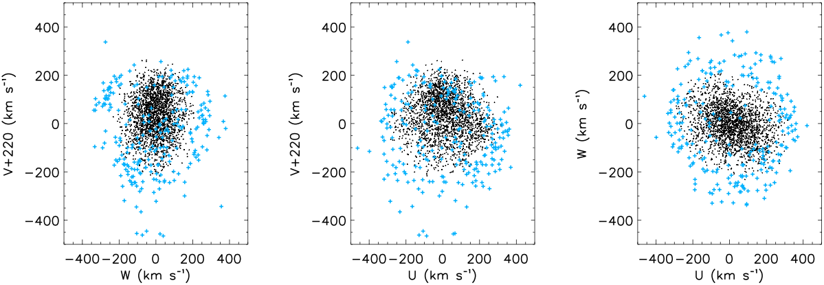
Figure 1.— Distribution of nearby halo stars in velocity space for our selected sample of $2417$ FGK subdwarfs, with $\rm{[Fe/H]<-1.5}$ and $|z|>1$ kpc within $3$ kpc of the Sun. The $10\%$ fastest-moving stars ($242$) are marked as crosses.

3.1. Local halo velocity distribution

From the selected sample we measure the mean velocities $(\langle U\rangle,\langle V+220\rangle,\langle W\rangle)$, the velocity ellipsoid $(\sigma_{U},\sigma_{V},\sigma_{W})$, and the correlations among velocity components ($\rho_{UV},\rho_{UW},\rho_{VW})$ as reported in Table 1.

The kinematic properties of the selected tracers are representative of the halo population in the vicinity of the Sun (e.g., Chiba & Beers, 2000).

The significant correlation $\rho_{UW}=-0.18\pm 0.02$ between the radial and vertical velocity components indicates a tilt of the velocity ellipsoid (Fig. 1, right panel).

Using the tilt formula (see, e.g., Binney & Merrifield, 1998)

$$\tan{2\delta_{UW}}=\frac{2~{}\sigma^{2}_{UW}}{\sigma^{2}_{U}-\sigma^{2}_{W}}=\frac{2~{}\rho_{UW}~{}\sigma_{U}\sigma_{W}}{\sigma^{2}_{U}-\sigma^{2}_{W}},$$ (1)

and the values in Table 1 for the correlation coefficient and velocity dispersions along the $U$ and $W$ axes, we derive a tilt angle of $\delta_{UW}=-14.5^{\circ}\pm 1.4^{\circ}$, revealing that the $(U,W)$ distribution points toward the Galactic center.

In fact, for our halo sample of 2417 FGK subdwarfs with $\langle z\rangle\approx$ 1.2 kpc and $\langle R\rangle\approx 8.3$ kpc, we estimate a mean position angle $\langle\tan^{-1}(z/R)\rangle~{}\approx 8.3^{\circ}$. This result is fairly consistent with the tilting effects on the velocity ellipsoids due to the gravitational potential produced by the stellar disk and dark matter halo (Bond et al., 2010, and references therein). We also measure smaller but stastistically significant correlations in $(U,V)$ and $(V,W)$ velocity-planes.

In the following, we look for halo streamers in the high velocity tail of the $(U,V,W)$ velocity distribution, where kinematic substructures are more easily detected. In order to select high velocity stars, we model the velocity distribution as a tilted Schwarzschild ellipsoid:

$$\begin{array}[]{lll}f(U,V,W)&=&{\rm const}\,\cdot e^{-\frac{1}{2}E(U,V,W)}\end{array}$$ (2)

where $E$ is the velocity function defined by:

$$\begin{array}[]{lll}&&\hbox to0.0pt{$\displaystyle E(U,V,W)=$\hss}\\ &&\\ &&\frac{R_{UU}}{R}\left(\frac{U-\langle U\rangle}{\sigma_{U}}\right)^{2}+\frac{R_{VV}}{R}\left(\frac{V-\langle V\rangle}{\sigma_{V}}\right)^{2}+\frac{R_{WW}}{R}\left(\frac{W-\langle W\rangle}{\sigma_{W}}\right)^{2}+\\ &&\\ &&2\frac{R_{UV}}{R}\left(\frac{U-\langle U\rangle}{\sigma_{U}}\right)\left(\frac{V-\langle V\rangle}{\sigma_{V}}\right)+\\ &&\\ &&2\frac{R_{VW}}{R}\left(\frac{V-\langle V\rangle}{\sigma_{V}}\right)\left(\frac{W-\langle W\rangle}{\sigma_{W}}\right)+\\ &&\\ &&2\frac{R_{UW}}{R}\left(\frac{U-\langle U\rangle}{\sigma_{U}}\right)\left(\frac{W-\langle W\rangle}{\sigma_{W}}\right).\end{array}$$ (3)

Here, $R$ represents the determinant of the symmetrical matrix $\mathcal{R}$ of the correlation coefficients $\rho_{ij}=R_{ij}/R$ (for $i,j=U,V+220,W$), and $R_{ij}$ designate the cofactor of the corresponding correlation element in $\mathcal{R}$ (e.g., Trumpler & Weaver, 1953).

Figure 1 shows the kinematic distribution for the individual components, $(U,V+220,W)$, of the space-velocity vector for the full sample of $2417$ selected halo stars; the $242$ objects comprising the sample of the $10\%$ highest velocity tail are represented with crosses.

As expected, the overall velocity distribution is relatively smooth, because of the strong phase-mixing that takes place in the inner-halo region, and slowly prograde (e.g., Helmi, 2008).
However, as their motions (in direction and speed) are well separated from those of the other nearby subdwarfs, we intend to study the degree of clumpiness of the $10\%$ fastest-moving objects. The case study is that, of all the objects passing within a few kiloparsecs of the Sun, some are part of a diffuse local stellar halo, while some could be debris of accretion events and remnants from the outer-halo population currently in the Solar Neighbourhood.

Before starting to look for kinematic substructures, we check for thick disk stars that possibly contaminate our halo tracers. Here, we applied to kinematic method described in Spagna et al. (2004) and estimate the fraction of subdwarfs that is consistent with the 3D velocity distribution of the thick disk population. By assuming a velocity ellipsoid, as estimated by Pasetto et al. (2012), and a rotation velocity $V_{\phi}=150$ km s^-1, as measured by Spagna et al. (2010a) for metal-poor thick disk stars with $\rm{[Fe/H]}\simeq-1$ dex, we found at a $2\sigma$ (i.e. $87\%$) confidence level a $\sim 10\%$ maximum contamination of thick disk in the whole sample of 2417 halo tracers. Instead, no contaminant is expected among the subsample of the $10\%$ fastest objects.

We use the samples described above to detect and subsequently identify kinematic halo substructures in the Solar Neighbourhood as groups of stars moving with similar velocities and directions. Detection is accomplished by performing a statistical test based on individual kinematics aimed at quantifying possible deviations from a smooth distribution of the background halo; cluster analysis in velocity space is then applied for final confirmation of the substructures.

3.2. The two-point correlation function: finding the clumps

The amount of kinematic substructures that cosmology might leave in the volume is quantified by means of the cumulative two-point correlation function, $\xi({\bf v})$, on the paired velocity difference ${\bf v}=|{\bf v}_{i}-{\bf v}_{j}|$ that measures the excess in the number of stellar pairs moving within a given velocity difference when compared to a representative random smooth sample (cfr. Re Fiorentin et al., 2005, for more details). Here the random points were drawn from a multivariate distribution obtained from the observed data set by random permutations of the order of the velocity components $V+220$ and $W$, after fixing $U$; finally, the actual random pairs are obtained after averaging over ten independent realisations.

This function is computed over the full sample of $2417$ halo stars, and separately for the sub-sample of the $242$ fastest-moving stars, corresponding to the $10\%$ high-velocity tail.

A statistical excess of stars with small pairwise velocity differences indicates the presence of likely streamers made of objects with coherent kinematics.

Figure 2 shows, using bins of $10~{}\rm{km\,s^{-1}}$ width the two-point correlation function $\xi({\bf v})$ for the full sample of $2417$ halo stars (dots) and for the subset of the $10\%$ fastest-moving stars (diamonds). While weak for the full sample, there is a statistically significant signal ($SNR>4$) for the subset of the fastest stars, that peaks at $40~{}\rm{km\,s^{-1}}$: the excess of pairs of stars with similar velocities is very noticeable, and is a direct indication of the presence of kinematical clumps.

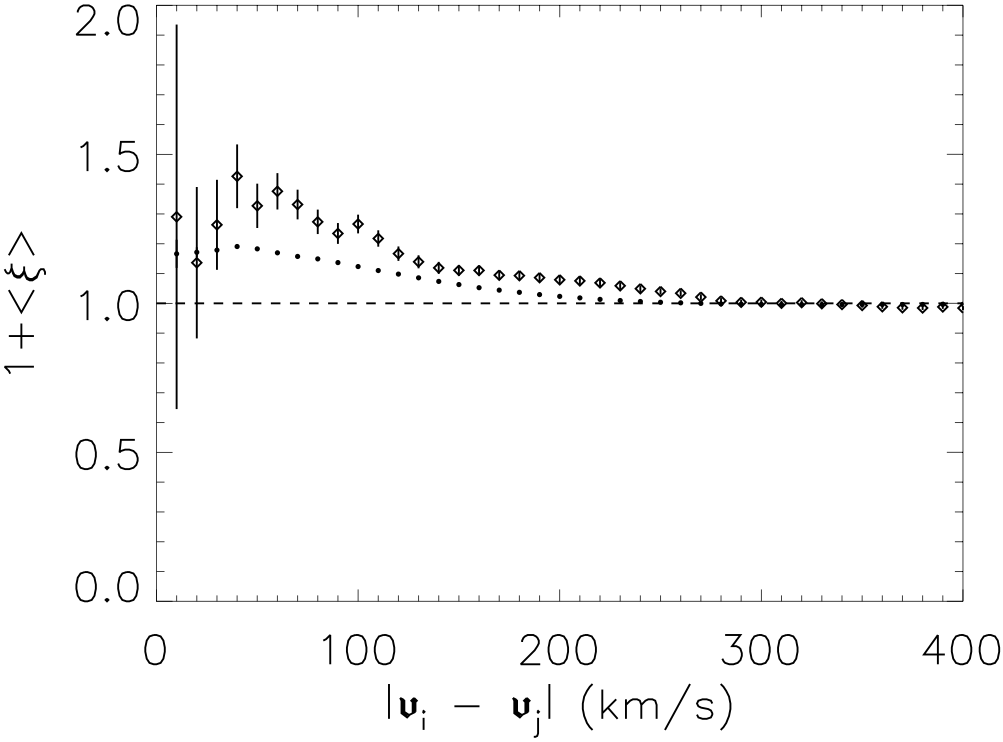
Figure 2.— Cumulative velocity correlation function for the full sample of halo stars (dots), and the $10\%$ fastest-moving subset (diamonds) shown in Fig. 1. The error bars are derived from Poisson’s statistics of the counts.

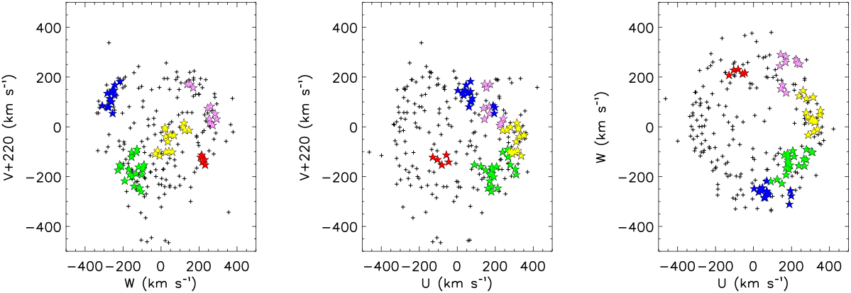
Figure 3.— Distribution of the high-velocity tail from our selected sample with $\rm{[Fe/H]<-1.5}$ and $\rm{|z|>1}$ kpc within $3$ kpc of the Sun (see Fig. 1). Shown are $242$ objects, the $10\%$ fastest-moving stars. Among them, star symbols identify the $67$ sources with pairwise velocity differences below $40~{}\rm{km~{}s^{-1}}$; the stars belonging to isolated pairs have been excluded. Different colours are used to indicate stars associated with the five clumps recovered by the clustering analysis.

In the following, among the sample of the $242$ fastest stars, we focus on the objects with paired velocity differences less than $40~{}\rm{km\,s^{-1}}$, which yield the statistically significant signal seen in Fig. 2. In addition, we exclude isolated pairs, i.e., “groups” with only two objects. This further selection certainly reduces the number of detected members, however it makes the following analysis more robust by decreasing the contamination of false positives. The final sample is made of $67$ stars.

3.3. Clustering analysis: assigning membership

In order to classify these $67$ objects, we perform $K-$medoids clustering in the 3D velocity space that defines the number of kinematic substructures and their members. This unsupervised learning algorithm is able to group data into a pre-specified number of clusters that minimises the RMS of the distance (in velocity space) to the center of each cluster.

The original data set is initially partitioned into clusters around $K$ data points referred to as the medoids, then an iterative scheme (PAM, for Partitioning Around Medoids) is applied to locate the medoids that achieve the lowest configuration “cost”. The algorithm employed by PAM, similar to the $K$-means clustering algorithm, is more robust to outliers and obtains a unique partitioning of the data without the need for explicit multiple starting points for the proposed clusters (see, e.g., Kaufmann & Rousseeuw, 1990; Hastie et al., 2001).

There is no general theoretical solution for finding the optimal number of clusters for any given data set. Increasing $K$ results in the error function values formally much smaller, but this increases the risk of overfitting. In order to keep the final identification safe and simple, we compared the results of runs with different $K$ classes, and the best $K$ resulted following visual inspection of the generated distribution. The solution adopted here is with $K=5$: for $K<5$ the clusters returned by the algorithm would contain a mixture of the natural underlying groups (e.g., prograde and retrograde members in the same kinematic clump); for $K>5$ natural groups further partition into “artificial” subgroups.

The five kinematic substructures detected are visualised in Fig. 3 with different colours.

The individual kinematic properties of the $67$ stars belonging to the five kinematics groups are listed in Table 2.

Other methods have been utilised to isolate groups of stars in the halo like, e.g., the interesting approach specifically developed for the Virgo stellar stream by Duffau et al. (2014). On the other hand, the fact that we have the complete set of 3D kinematical data and that the whole sample is confined within $3$ kpc from the Sun (i.e., the distance segregation is implicitly implemented in our sample) suggests the direct use of a classical clustering algorithm like PAM as the method of choice.

3.4. Angular momentum and orbital properties

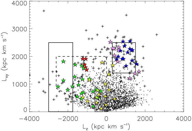
Figure 4.— Distribution of the selected sample of $2417$ FGK subdwarfs within $3$ kpc of the Sun in the space of adiabatic invariants. Cross symbols indicate the $10\%$ fastest-moving objects. Among them, star symbols identify the $67$ sources with paired velocity differences below $40~{}\rm{km~{}s^{-1}}$. As in Fig. 3, different colours are used to indicate stars associated with the five clumps recovered by the clustering analysis in velocity space. At $L_{z}>0$, the solid box shows the locus of the halo stream discovered by Helmi et al. (1999): the kinematic substructures, pink and blue stars (i.e., Groups 1 and 2 in Table 2), on prograde orbits indeed cover the same region. At $L_{z}<0$, the solid box at $L_{z}\sim-2375$ shows the locus of the substructure detected by Kepley et al. (2007) as retrograde outliers, while the solid contour at $L_{z}\sim-400$ identifies the $\omega$ Cen substructures remapped from the $L_{z}$-$L$ region in Dinescu (2002). The area within the dashed line includes the kinematic Groups 3, 4, and 5 of Table 2, represented by the red, green, and yellow stars, respectively.

The space of adiabatic invariants allows better identification of the different possible merging events that might have given rise to the observed substructures. Clumping should be even stronger, since all stars originating from the same progenitor should have very similar integrals of motion, resulting in a superposition of the corresponding streams; that is, the initial clumping of satellites are present even after the system has completely phase-mixed (e.g., Helmi & de Zeeuw, 2000).

In this study we focus on the plane defined by the components of angular momentum in and out the plane of the Galaxy’s disk, i.e. $L_{xy}$ and $L_{z}$ respectively.

Since for a local sample $(x,y,z)\sim(r_{\sun},0,0)$, we remark that $L_{xy}\sim r_{\sun}|v_{z}|$ is dominated by the velocity perpendicular to the plane and $L_{z}\sim r_{\sun}v_{y}$ measures the amount of rotation of a given stellar orbit. Essentially, stars with high/low $L_{xy}$ are on high/low-inclination orbits; stars with $L_{z}<0$ are on retrograde orbits and stars with $L_{z}>0$ are on prograde orbits.

Figure 4 shows the distribution of the selected sample within $3$ kpc of the Sun in the angular momentum diagram $L_{z}$ versus $L_{xy}$. As in Fig. 3, the $10\%$ fastest-moving objects are plotted as crosses, and with the star symbols we mark the group members identified in Sect. 3.2. Different colours indicate the stars associated with the different lumps recovered by the cluster analysis in velocity space.

The solid lines show the loci of the known kinematic structures detected by

1. Helmi et al. (1999) at
   $300<L_{z}<1500~{}\rm{kpc~{}km~{}s^{-1}}$ and
   $1400<L_{xy}<2500~{}\rm{kpc~{}km~{}s^{-1}}$,

2. Kepley et al. (2007) at
   $-3000<L_{z}<-1750~{}\rm{kpc~{}km~{}s^{-1}}$ and
   $0<L_{xy}<2500~{}\rm{kpc~{}km~{}s^{-1}}$,

3. Dinescu (2002) at
   $-600<L_{z}<-200~{}\rm{kpc~{}km~{}s^{-1}}$ and
   $0<L_{xy}<L_{xy}^{lim}~{}\rm{kpc~{}km~{}s^{-1}}.$

Table 2 Main individual characteristics of the $67$ fastest-moving stars found members of 5 different kinematics groups.

Group	ID	$U$	$V+220$	$W$	$L_{xy}$	$L_{z}$	$\rm{[Fe/H]}$
		$\rm{(km~{}s^{-1})}$	$\rm{(km~{}s^{-1})}$	$\rm{(km~{}s^{-1})}$	$\rm{(kpc~{}km~{}s^{-1})}$	$\rm{(kpc~{}km~{}s^{-1})}$	(dex)
1a / pink	52209-0694-596	$143\pm 14$	$33\pm 12$	$293\pm 6$	$2289$	$389$	$-2.01$
	52721-1050-418	$145\pm 7$	$173\pm 6$	$155\pm 4$	$1390$	$1473$	$-2.02$
	53315-1907-393	$170\pm 31$	$54\pm 31$	$285\pm 16$	$2232$	$614$	$-1.75$
	53349-2066-511	$154\pm 23$	$158\pm 28$	$169\pm 27$	$1459$	$1678$	$-1.85$
	54175-2472-370	$139\pm 13$	$76\pm 16$	$246\pm 4$	$2336$	$634$	$-1.75$
	54574-2904-114	$243\pm 9$	$35\pm 9$	$254\pm 3$	$2301$	$316$	$-1.94$
	54577-2906-088	$225\pm 12$	$8\pm 12$	$272\pm 5$	$2532$	$198$	$-2.16$
	54621-2191-177	$231\pm 11$	$16\pm 11$	$257\pm 10$	$2045$	$405$	$-1.81$
	54624-2189-236	$169\pm 17$	$84\pm 26$	$261\pm 23$	$1820$	$590$	$-1.73$
	54629-2902-237	$172\pm 7$	$172\pm 9$	$138\pm 6$	$1216$	$1203$	$-2.64$
2a / blue	52316-0559-336	$189\pm 3$	$87\pm 11$	$-310\pm 5$	$2545$	$853$	$-2.52$
	53084-1368-399	$195\pm 5$	$55\pm 6$	$-255\pm 4$	$1906$	$517$	$-2.16$
	53242-1896-109c	$41\pm 14$	$149\pm 11$	$-256\pm 7$	$2220$	$1299$	$-1.66$
	53262-1900-359	$62\pm 19$	$82\pm 21$	$-283\pm 17$	$2215$	$706$	$-2.09$
	53293-1906-633c	$27\pm 6$	$139\pm 7$	$-261\pm 5$	$2281$	$1210$	$-1.91$
	53467-2110-134	$69\pm 10$	$102\pm 11$	$-260\pm 3$	$1921$	$815$	$-1.55$
	53712-2314-639	$75\pm 5$	$103\pm 6$	$-265\pm 5$	$2387$	$936$	$-2.57$
	53726-2306-188c	$55\pm 9$	$136\pm 10$	$-283\pm 7$	$2555$	$1218$	$-1.74$
	53907-2209-540c	$70\pm 13$	$144\pm 12$	$-256\pm 13$	$1663$	$1011$	$-2.30$
	54178-2452-540	$70\pm 6$	$184\pm 7$	$-216\pm 3$	$1735$	$1556$	$-1.51$
	54380-2323-448	$47\pm 15$	$170\pm 13$	$-243\pm 13$	$1858$	$1324$	$-2.12$
	54479-2867-531	$33\pm 14$	$129\pm 11$	$-246\pm 12$	$2153$	$1097$	$-1.64$
	54530-2889-458	$3\pm 4$	$148\pm 9$	$-247\pm 4$	$2238$	$1342$	$-1.56$
	54554-2918-615	$198\pm 15$	$80\pm 15$	$-276\pm 3$	$2004$	$604$	$-1.98$
	54580-2905-169	$80\pm 10$	$115\pm 11$	$-271\pm 4$	$1923$	$873$	$-1.71$
3b / red	54179-2567-458	$-57\pm 12$	$-112\pm 16$	$214\pm 8$	$1922$	$-1076$	$-1.64$
	54463-2856-571	$-129\pm 9$	$-121\pm 22$	$209\pm 6$	$1617$	$-1089$	$-2.09$
	54551-2394-228	$-104\pm 10$	$-130\pm 14$	$230\pm 8$	$1924$	$-1234$	$-1.72$
	54562-2920-596	$-81\pm 19$	$-152\pm 19$	$232\pm 10$	$1521$	$-1032$	$-2.36$
	54569-2900-046	$-46\pm 7$	$-139\pm 8$	$218\pm 3$	$1712$	$-1139$	$-1.68$
4b / green	52059-0597-072	$125\pm 4$	$-157\pm 10$	$-210\pm 6$	$1672$	$-1280$	$-2.09$
	52338-0788-070	$180\pm 9$	$-237\pm 11$	$-142\pm 9$	$921$	$-1767$	$-2.07$
	52942-1509-488	$179\pm 9$	$-259\pm 22$	$-105\pm 8$	$1137$	$-2235$	$-1.64$
	53710-2310-141	$207\pm 39$	$-159\pm 16$	$-95\pm 20$	$1195$	$-877$	$-1.60$
	53762-2381-588	$213\pm 16$	$-244\pm 29$	$-117\pm 14$	$916$	$-2517$	$-1.85$
	53800-2383-625	$172\pm 7$	$-190\pm 14$	$-164\pm 8$	$1275$	$-1652$	$-1.69$
	53823-2240-213	$310\pm 22$	$-190\pm 26$	$-100\pm 4$	$557$	$-1513$	$-1.70$
	53874-2173-414	$279\pm 16$	$-151\pm 18$	$-89\pm 12$	$199$	$-688$	$-1.57$
	54154-2701-341	$171\pm 10$	$-216\pm 16$	$-191\pm 21$	$1826$	$-2236$	$-1.74$
	54169-2413-090	$149\pm 12$	$-172\pm 12$	$-226\pm 7$	$1711$	$-1626$	$-1.77$
	54234-2663-321	$90\pm 11$	$-151\pm 13$	$-218\pm 3$	$1581$	$-1187$	$-2.16$
	54539-2894-314	$162\pm 3$	$-244\pm 12$	$-112\pm 5$	$793$	$-2008$	$-2.12$
	54539-2894-632	$305\pm 6$	$-168\pm 6$	$-99\pm 3$	$478$	$-1299$	$-1.59$
	54544-2459-072	$239\pm 7$	$-100\pm 8$	$-154\pm 7$	$802$	$-532$	$-1.82$
	54557-2177-009	$277\pm 16$	$-100\pm 18$	$-130\pm 10$	$507$	$-454$	$-2.73$
	54568-2899-316	$182\pm 17$	$-160\pm 25$	$-117\pm 4$	$665$	$-1294$	$-1.92$
	54595-2932-091	$268\pm 17$	$-120\pm 15$	$-156\pm 7$	$737$	$-704$	$-1.63$
	54597-2561-326	$265\pm 15$	$-89\pm 3$	$-127\pm 4$	$750$	$-289$	$-1.96$
	54616-2460-420	$186\pm 8$	$-169\pm 9$	$-169\pm 9$	$1180$	$-1246$	$-1.93$
	54616-2460-616	$192\pm 16$	$-199\pm 15$	$-152\pm 16$	$977$	$-1450$	$-1.98$
	54631-2911-151	$182\pm 11$	$-187\pm 11$	$-132\pm 8$	$710$	$-1212$	$-1.96$
5b / yellow	53035-1433-600	$322\pm 10$	$-8\pm 13$	$22\pm 6$	$1004$	$-56$	$-1.58$
	53240-1894-079	$277\pm 22$	$-99\pm 18$	$59\pm 18$	$120$	$-273$	$-2.10$
	53315-1907-353	$352\pm 35$	$-33\pm 35$	$68\pm 18$	$258$	$-32$	$-1.50$
	53770-2387-010	$322\pm 6$	$-2\pm 12$	$21\pm 4$	$559$	$-66$	$-1.67$
	53848-2437-060	$314\pm 13$	$17\pm 22$	$121\pm 13$	$1787$	$-228$	$-2.18$
	53876-2134-516	$318\pm 13$	$-94\pm 13$	$-17\pm 5$	$528$	$-518$	$-1.52$
	53918-2539-196	$240\pm 10$	$-13\pm 8$	$126\pm 8$	$1356$	$121$	$-1.93$
	54082-2325-126	$278\pm 23$	$0\pm 16$	$115\pm 15$	$468$	$420$	$-1.61$
	54156-2393-459	$336\pm 11$	$-115\pm 9$	$-8\pm 5$	$527$	$-1231$	$-1.74$
	54243-2176-476	$350\pm 6$	$-32\pm 4$	$50\pm 4$	$795$	$131$	$-1.73$
	54271-2449-590	$261\pm 11$	$-12\pm 9$	$147\pm 7$	$1686$	$321$	$-2.21$
	54368-2804-351	$302\pm 15$	$-100\pm 19$	$24\pm 19$	$332$	$-523$	$-1.67$
	54536-2871-426	$286\pm 21$	$-97\pm 40$	$42\pm 11$	$1155$	$-888$	$-1.93$
	54594-2965-227	$288\pm 14$	$-107\pm 16$	$-31\pm 6$	$387$	$-974$	$-1.64$
	54594-2965-272	$328\pm 14$	$-37\pm 12$	$25\pm 5$	$782$	$-448$	$-1.54$
	54616-2929-342	$310\pm 7$	$-58\pm 8$	$36\pm 2$	$625$	$-403$	$-1.60$

Note. — Main individual characteristics of the $67$ selected fastest-moving stars with paired velocity differences less than $40\,\rm{km\,s^{-1}}$, and belonging to 5 different kinematics groups. These are 25 subdwarfs (21 new) on 2 streamers (Group 1 and Group 2) both members of the stream known to Helmi et al. (1999) originally made of red giants and RR Lyrae. The remaining $42$ are subdwarfs members of three newly discovered kinematic groups (Group 3, 4, and 5); see text for their dynamical interpretation.

The most noticeable feature in Fig. 4 is certainly the kinematic group corresponding to the stream found by Helmi et al. (1999). Here, we identify $25$ subdwarfs, including $4$ stars already detected by Klement et al. (2009), and $21$ new members. By inspection of Fig. 3 we notice that the $10$ members belonging to Group 1 (pink star symbols) run along near-parallel orbits and cross the Milky Way’s disk at high speed from South to North, and the $15$ objects in Group 2 (blue star symbols) cross the Milky Way’s disk at similar speed and angle, but from North to South.

The three remaining lumps of fast-moving stars (red Group 3, green Group 4, and yellow Group 5) appear on the retrograde side of Fig. 4. The pentagonal box confined by the dashed line includes most of the members of Group 3 ($5$ stars), Group 4 ($21$ stars), and Group 5 ($16$ stars).

These groups, and in particular the small Group 3, do not appear to be easily associated with known streams and, in Sect. 5, we discuss the possibility that all these stars come from a common progenitor or from three different merging events.

Anyhow, we note that Group 4 might be the parent populations of the counter-rotating “outliers”, with $V_{\phi}<-250~{}\rm{km~{}s^{-1}}$, found by Kepley et al. (2007), while the slightly retrograde Group 5 ($V_{\phi}\approx-50~{}\rm{km~{}s^{-1}}$) seems to be related to the kinematic structure found by Dinescu (2002), and confirmed by both Meza et al. (2005) and Majewski et al. (2012). These authors have also discussed the possibility that such a stream is formed by the tidal debris of $\omega$ Cen in the solar neighborhood, even though Navarrete et al. (2015) have recently ruled out this hypothesis after detailed analysis of the chemical abundance of this group with respect to the well-known peculiar properties of $\omega$ Cen.

4. Simulations

We explore a simulated inner halo based on a set of four high-resolution numerical N-body simulations of minor mergers. We analyse the kinematics and orbital properties of these simulations in order to investigate and characterise detectable signatures.

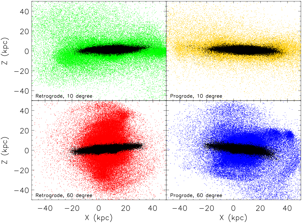
Figure 5.— Final configurations in the $(x,z)$ plane of four minor merger events: depicted are the morphologies of the stellar distribution, i.e. the host disk (black) and the satellite bulge (colour), at the final time $T=4.63$ Gyr of the simulations. Shown are the cases of low-inclination ($10^{\circ}$ tilt) retrograde (top left) / prograde (top right) orbit, and of high-inclination ($60^{\circ}$ tilt) retrograde (bottom left) / prograde (bottom right) orbit. The panels only display a randomly selected $10\%$ subset of the total particles utilised.

It is useful to point out that these simulations are not an attempt to “fit” the observations, but they represent four merging events that we assume as representative, in terms of inclination and rotation, of the initial orbits of the satellites. In particular, these choices allow us to analyse the two cases suffering maximum and minimum dynamical friction.

4.1. N-body simulations

We use a set of high-resolution numerical N-body simulations which simulate minor mergers of prograde and retrograde orbiting satellite halos within a dark matter main halo (Murante et al., 2010). The main DM halo, which contains a stellar, rotating exponential disk, has a NFW radial density profile (Navarro, Frenk & White, 1997), with a mass ($M_{200}=10^{12}$ M_☉), radius ($R_{200}=165$ kpc), and concentration ($C_{200}=7.5$), appropriate for a Milky Way-like DM halo at redshift $z=0$; the spin parameter is set to $\lambda=1$. The satellite is represented by a secondary DM halo containing a stellar bulge, and a Hernquist radial density profile (Hernquist, 1993); the spin parameter is set to $\lambda=0$. The mass ratio, $M_{\rm primary}/M_{\rm satellite}\sim 40$, is similar to the estimated mass ratio of the Milky Way relative to the Large Magellanic Cloud. The main physical parameters of our simulated mergers are listed in Table 3.

We consider prograde mergers, in which the satellite co-rotates with the spin of the disk, as well as retrograde mergers, with a counter-rotating satellite. We analyse two orbits: a low-inclination orbit with a $10^{\circ}$ tilt with respect to the disk plane, and a high-inclination orbit with a $60^{\circ}$ tilt.

Initially, the particles of the small system (satellite galaxy) orbiting around the (otherwise static) disk galaxy are all strongly concentrated in space, and share essentially the same motion. The initial conditions (inclination, position, and velocity) of the main system and the four impacting satellites, cosmologically motivated (Read et al., 2008; Villalobos & Helmi, 2008), are summarised in Table 4.

From the grid of simulations by Read et al. (2008), we chose four impactors, all of which having the mass of the Large Magellanic Cloud. Larger masses would affect the stability of the stellar disk, and this is not consistent with a Milky Way-like galaxy. Conversely, smaller masses would produce minor signatures in our local halo sample.

The four simulations are compiled using the public parallel Treecode GADGET2 (Springel, 2005) on the cluster matrix at the CASPUR (Consorzio Interuniversitario per le Applicazioni del Supercalcolo) consortium, Rome. All systems were left to evolve for $4.63$ Gyr (about $16$ dynamical timescales of the main halo). After this time, the four satellites have completed their merging with the primary halo. The final $(x,z)$ distribution of the inner satellite star particles and host disk, in both the retrograde and prograde cases, as well as for the high and low inclinations, is shown in Fig. 5.

Table 3 Physical properties of the Halos: Main system and orbiting Satellite.

System	$M_{DM}$	$M_{*}$	$N_{DM}$	$N_{*}$	$r_{0}$	$r_{disk}$
Main	$10^{12}$	$5.7\times 10^{10}$	$10^{6}$	$10^{6}$	4	20
Satellite	$2.4\times 10^{10}$	$2.4\times 10^{9}$	$1.1\times 10^{5}$	$10^{5}$	0.709	…

Note. — Column 1: Main galaxy/Impacting system. Column 2: DM mass, in $M_{\sun}$. Column 3: stellar mass for disk/bulge in the main/satellite, in $M_{\sun}$. Column 4: DM particles. Column 5: stellar particles for disk/bulge in main/satellite. Column 6: disk scale radius for the main halo, in kpc; Hernquist scale radius for the satellite, in kpc. Column 7: disk truncation radius, in kpc.

Table 4 Initial conditions of the Main system and the four impacting Satellites.

System	Inclination	Rotation	$x$	$y$	$z$	$v_{x}$	$v_{y}$	$v_{z}$	$v$
			(kpc)	(kpc)	(kpc)	$\rm{(km~{}s^{-1})}$	$\rm{(km~{}s^{-1})}$	$\rm{(km~{}s^{-1})}$	$\rm{(km~{}s^{-1})}$
Main	$0^{\circ}$	$-$	0.00	$0.00$	$0.00$	$0.00$	$0.00$	$0.00$	$0.00$
Satellite 1	$10^{\circ}$	retrograde	$80.00$	$0.27$	$15.20$	$6.30$	$-62.50$	$0.35$	$62.82$
Satellite 2	$10^{\circ}$	prograde	$80.00$	$0.27$	$15.20$	$6.30$	$62.50$	$0.35$	$62.82$
Satellite 3	$60^{\circ}$	retrograde	$15.00$	$0.12$	$26.00$	$1.20$	$80.10$	$2.00$	$80.13$
Satellite 4	$60^{\circ}$	prograde	$15.00$	$0.12$	$26.00$	$1.20$	$-80.10$	$2.00$	$80.13$

Note. — Inclination and rotation of the orbit, position and velocity components, and total velocity.

4.2. Dynamical friction and tidal stripping

Any satellite can in principal be slowed by dynamical friction exerted on it by disk and halo particles. It is known that an object, such as a satellite, of mass $M$, moving through a homogeneous background of individually much lighter particles with an isotropic velocity distribution suffers a drag force (Chandrasekar, 1943):

$$F_{d}=-\frac{4\pi G^{2}M^{2}\rho_{f}(<v_{s})\ln\Lambda}{v_{s}^{2}},$$

where $v_{s}$ is the speed of the satellite with respect to the mean velocity of the field, $\rho_{f}(<v_{s})$ is the total density of the field particles with speeds less than $v_{s}$, and $\ln\Lambda$ is the Coulomb logarithm (Binney & Tremaine, 1987).

We expect that, the higher the $v_{s}$, the weaker is the dynamical friction force. Retrograde satellites are expected to suffer weaker dynamical friction with respect to prograde ones, since in the first case the velocity of the satellite is opposite to that of the disk. As a consequence, prograde orbits decay faster. This effect is even more evident for low-inclination orbits.

Another important effect that occurs during mergers is the tidal disruption of satellites. While tidal disruption is most important near the centre of the main halo, where the gravitational potential is changing more rapidly, dynamical friction is exerted both by the main halo DM particles and by the disk star particles.

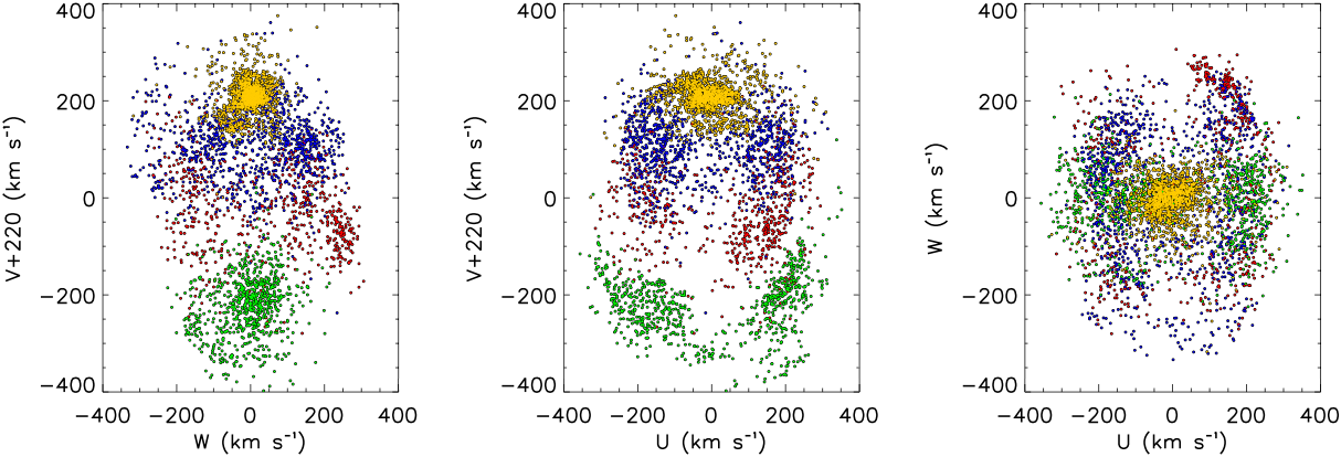
Figure 6.— Kinematical (velocity space) distribution of the accreted component of the simulated Milky Way inner halo, i.e., $3902$ particles in a spherical volume of radius $3$ kpc centered on the “Sun” with $|z|>1$ kpc. Different colours indicate particles associated with different satellites: $60^{\circ}$ retrograde/prograde (red/blue), $10^{\circ}$ retrograde/prograde (green/yellow) colliding satellites.

4.3. Debris in the local halo

We analyse the observational signature left by the satellite stars after selecting particles in a sphere of $3$ kpc radius centered at the Sun ($x=8$ kpc from the Galaxy center), and with $|z|>1$ kpc. This last constraint is introduced so that the simulated and observed samples can be compared within a similar volume of the inner halo.

Figure 6 shows the kinematic distribution (velocity projections) of our simulated inner halo. The different colours indicate the association of the 3902 debris stars with different progenitors: the low/high-inclination retrograde satellites (761/616 green/red dots), and the high/low-inclination prograde satellites (966/1559 blue/yellow dots).

The angular momentum distribution of the satellite debris is shown in Fig. 7. Despite the chaotic build up of the parent halo, it appears that objects from accreted satellites remain confined in limited portions of the $(L_{z},L_{xy})$ plane.

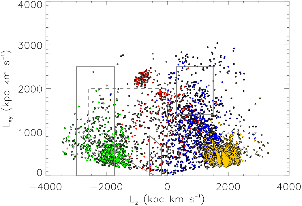
Figure 7.— Angular momentum distribution of the simulated Milky Way halo within $3$ kpc of the “Sun”. As in Fig. 6, shown are the $3902$ particles accreted from four dwarf galaxies: $60^{\circ}$ retrograde/prograde (red/blue), $10^{\circ}$ retrograde/prograde (green/yellow) satellites after interaction with the simulated Milky Way. All of the marked regions have the same meaning as in Fig. 4.

The satellite on a low-inclination prograde orbit (yellow particles), which suffers more from dynamical friction, quickly loses its orbital energy and proceeds to the inner regions of the main halo (Byrd et al., 1986; Murante et al., 2010). For this reason less particles are left in the outer-halo, see top-right panel of Fig. 5.

It is worth noticing that the high inclination prograde satellite suffers the effect of dynamical friction as well, as a result of its co-rotation with the disk. This effect acts in producing a consistent mass of debris in the solar region having $L_{xy}$ ranging between $500$ $\rm{kpc~{}km~{}s^{-1}}$ and $1500$ $\rm{kpc~{}km~{}s^{-1}}$ (blue points in Fig. 7).

On the other hand, retrograde satellites experience weaker dynamical friction and leave more particles in the outer-halo region, since their orbits have a longer decay time and longer periods. Thus, tidal stripping (see e.g., Colpi et al., 1999) can act longer and more efficiently when the satellite is still orbiting at high velocity, and we see that a better populated high-velocity tail results (compare Fig. 7 to Fig. 10).

The impact of dynamical friction on the two configurations considered for the retrograde satellites indicates that the high-inclination case is the one less affected by this force, which again results in efficient stripping when the satellite has high orbital velocity. Therefore, such stripping takes place over a large spatial region, and for the conservation of 6D phase-space density, by virtue of Liouville’s Theorem, we expect a small variance in velocity space and in the plane of angular momenta. This is indeed observed for the red particles with respect to the green ones in Figs. 6 and 7.

Finally, the effect of both gravitational feedback and dynamical friction on the satellites, which lead to loss of stars at different passages with different energies, is clearly evident for the case of low inclination prograde orbit in Fig. 7 at around $L_{xy}=400~{}\rm{kpc~{}km~{}s^{-1}}$ and $L_{z}=1750~{}\rm{kpc~{}km~{}s^{-1}}$.

5. “Observed” simulations

Here we investigate the effects of observational errors on our simulated data, and show how more accurate kinematic data to be provided by future surveys can improve detection and characterisation of halo streams. Moreover, we compare actual observations with the distributions of debris resulting from the four simulated satellites presented in the previous section, and discuss the orbital properties of the parent dwarf galaxies, possibly responsible for accreting on the Milky Way halo.

5.1. Observational errors

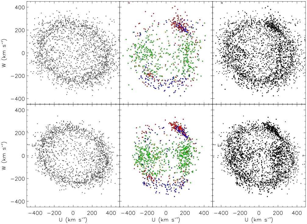
Figure 8.— The ($U$, $W$) velocity distribution of the $10\%$ high velocity tail of the simulated sample is shown in the right panels. The sample is limited to a spherical volume of radius 3 kpc located on the plane of the simulated Milky Way 8 kpc away from its center and with $|z|>1$ kpc. Of the 2874 particles in this sample, some are remnants of the four satellites accreted after 5 Gyr (middle panels), the remaining constitute the “background” of smooth inner halo stars (left panels). Different colours represent different progenitors as in Fig. 5. Finally, the top panels were generated via convolution with current, i.e. SGKS, ground-based errors, while the bottom figures depict the results after convolution with the expected Gaia-like errors.

We perturb the original simulations by convolving the “true” data with two cases of error distributions. First, we adopt the accuracy of our SGKS catalogue as representative of the quality of current wide-field surveys. Then, we assume the mean accuracy expected from the forthcoming Gaia catalogue combined with complementary deep spectroscopic data from on-going and future surveys such as GES (Gilmore et al., 2012).

The true positions and velocities of each particle are first transformed into their astronomical observables ($\alpha$, $\delta$, $m-M$, or $\pi$ and $\mu_{\alpha}$, $\mu_{\delta}$, $V_{r}$); then the expected observational errors are added to distance modulus (or directly to parallax, in the case of the Gaia-like simulation), radial velocity, and proper motion, according to Table 5.

The precision in distance is taken to $\sigma_{m-M}=0.4$ mag (i.e., $\sigma_{d}/d\simeq 20\%$) for the photometric distances estimated from the SGKS catalogue, and to $\sigma_{\pi}=20~{}\rm{\mu as}$ for the final precision on trigonometric parallaxes measured by Gaia. In proper motion, the precision is assumed to be $2~{}\rm{mas~{}yr^{-1}}$ for ground-based observations, and $20~{}\rm{\mu as~{}yr^{-1}}$ for Gaia. The precision in the radial velocity is taken to be $10~{}\rm{km~{}s^{-1}}$ for the SDSS measurements, and $1~{}\rm{km~{}s^{-1}}$ for the GES spectroscopic survey. These quantities are finally transformed back to observed positions vectors and space velocities.

Table 5 Estimated/Expected errors for the SGKS and Gaia catalogues.

Catalogue	distance	proper motion	radial velocity
SGKS	$\sigma_{m-M}=0.4$ mag	2000	10
Gaia/GES	$\sigma_{\pi}=20~{}\rm{\mu as}$	20	1

Note. — Estimated errors (precision) in parallax ($\sigma_{\pi}$, in $\rm{\mu as}$), distance modulus ($\sigma_{m-M}$, in mag), proper motion ($\sigma_{\mu}$, in $\rm{\mu as~{}yr^{-1}}$), and radial velocity ($\sigma_{V_{r}}$, in $\rm{km~{}s^{-1}}$) for the SGKS and Gaia catalogues.

Table 6 The composition of the 10% High Velocity Tail of the simulated Milky Way Halo.

Catalogue	Halo$+$Debris	Debris	Satellite 1	Satellite 2	Satellite 3	Satellite 4
“True” Simulation	2874	$1103~{}(0.38\%)$	262	201	601	39
“Observed” SGKS	2874	$835~{}(0.29\%)$	233	170	406	26
“Observed” Gaia/GES	2874	$1061~{}(0.37\%)$	263	191	570	37

5.2. The inner halo model

We explore a simulated inner halo based on the superposition of the four simulations of minor mergers and a smooth local component with the same kinematic properties of the observed sample (Table 1).

Consistently with the findings of Helmi et al. (1999) and Kepley et al. (2007), we assumed a debris total fraction of $10\%$ within $3$ kpc from the Sun.

In the “true” (simulated) catalogue, of the $28\,738$ particles with $|z|>1$ kpc, $24\,836$ are part of the local mock halo, while the remaining $3902$ are debris from the satellites shown in Figs. 6 and 7.

In the following discussion we focus on the particles of the accreted component that belong to the $10\%$ high velocity tail. Table 6 reports the number of particles belonging to each satellite for the pure simulation and the other two cases accounting for observational errors.

Figure 8 shows the region of the $(U,W)$ plane occupied by the $10\%$ high velocity tail of the resulting simulated Milky Way inner halo (right panels), as superposition the accreted component (middle panels) and the smooth spheroid (left panels). The synthetic “observed” catalogue shown in the top panels represent the current picture, according to the SGKS error model. The bottom panels show the distribution of the high velocity particles as promised by Gaia.

The upper panels indicate that distinguishing in velocity space the satellites that gave rise to each of the different moving groups with the extant data is a non-trivial task. On the other hand, as the inspection of the lower panels reveals, much of the substructures shown in the middle panels becomes visible again thanks to the superior precision that Gaia will achieve.

5.3. Substructures in the correlation function

In order to quantify the amount of kinematic substructures present among the 2874 fastest-moving particles, we compute the cumulative velocity correlation function described in Sect. 3.2. The analysis is performed over three synthetic catalogues: the “true” simulation, and two lists derived from the true values after perturbing them with either SGKS-like errors or the errors expected for the Gaia/GES surveys.

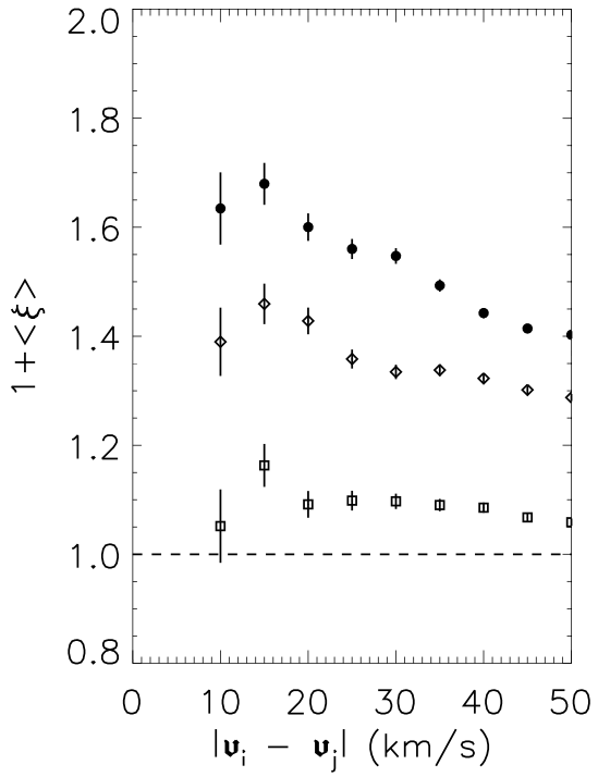
Figure 9.— The cumulative velocity correlation functions for the 2874 halo particles shown in Fig. 8. The filled dots trace the correlation function of the pure simulation, while squares and diamonds depict the correlation after convolution with current (i.e., SGKS) or Gaia/GES-like errors, respectively. Error bars are derived from Poisson’s statistics of the counts.

Figure 9 shows, using bins of width $\rm{5~{}km~{}s^{-1}}$ up to kinematical separations of $\rm{50~{}km~{}s^{-1}}$, the results for the two-point correlation function $\xi({\bf v})$ for the “true” case (dots), the SGKS-like (squares) and Gaia/GES-like (diamonds) catalogues. The clear signal in the first bins, peaking at $\Delta v\sim\rm{15~{}km~{}s^{-1}}$, evidences an excess of particles moving with similar velocities with respect to what expected from a fully random sample. In the case of the pure simulation, the two-point velocity correlation function attains a maximum signature of $\langle\xi\rangle=0.68\pm 0.04$. For the SGKS-like catalogue the maximum signal has an $\sim 80$% drop to an “observed” value of $\langle\xi\rangle=0.16\pm 0.04$.

The recovery of the intrinsic correlation signal is truly remarkable when looking at the correlation function for the Gaia-like case: in fact, we measure $\langle\xi\rangle=0.46\pm 0.04$, corresponding to $68\%$ of the original signal. Figure 8 provides a nice “visual” confirmation of the recovery in substructure visibility.

6. On the nature of the high velocity debris

As the space of adiabatic invariants is important to gain more insight into the properties of the kinematic substructures detected (Sect. 3.4), we compare the $(L_{z},L_{xy})$ distributions of the observed groups with the results of the simulations, taking into account the effect of the observational errors. This is shown in Fig. 10, where the top panel corresponds to the SGKS-error simulation, while the bottom panel reproduces what will hopefully be seen with the final Gaia catalogue.

The black star symbols in the upper panel of Fig. 10 represent the $67$ high velocity objects we found from our statistical analysis in the same volume and shown in Fig. 4 as colored stars. With current data, different satellites mix over some regions so that a discrete classification is not always straightforward. The bottom panel of Fig. 10 clearly shows that this situation is highly improved with Gaia-like data.

We see that our Groups 1 and 2, corresponding to the stream of Helmi et al. (1999), are consistently associated with the high inclination prograde satellite (blue dots). Because of dynamical friction (cfr. Sect. 4.3), this satellite includes a low $L_{xy}$ component shown in the full sample (Fig. 7) that is not part of the high velocity tail (Fig. 10). Thus, these simulated “observations” suggest the possible presence in the Helmi et al. (1999) stream of debris with lower $L_{xy}$ yet to be discovered.

Of particular interest is the case of the retrograde kinematic groups. In fact, neither the high-inclination simulated satellite nor the one at low-inclination appear to fairly match the observed Groups 3, 4, and 5, i.e. the black stars with $L_{z}\lesssim 0$ in Fig. 10.

Actually, these three groups appear to occupy an intermediate region between the debris of the two simulated retrograde satellites. Furthermore, in Sect. 3.4 we remark that the observed Groups 3, 4, and 5 do not well match the streams detected by Dinescu (2002) and Kepley et al. (2007). For this reason, we suggest that these three groups may represent the debris of an unique progenitor accreted along an initial retrograde orbit having an intermediate inclination in the range comprised between $10^{\circ}$ and $60^{\circ}$. In alternative, these groups could belong up to three different impacting satellites on retrograde orbits with inclinations in that same range.

The results presented in this section show that the methodology proposed is certainly capable of detecting fossil signatures as kinematic substructures among high-velocity stars. From the data at our disposal, there is clear indication that more debris are found from dwarf galaxies on high-inclination prograde and retrograde orbits, as well as on low-inclination retrograde ones. We have not identified any debris coming from low-inclination prograde satellites and this might be a limitation intrinsic to the methodology of looking at structures in the space motions of very high velocity stars. Future work will have to investigate these issues.

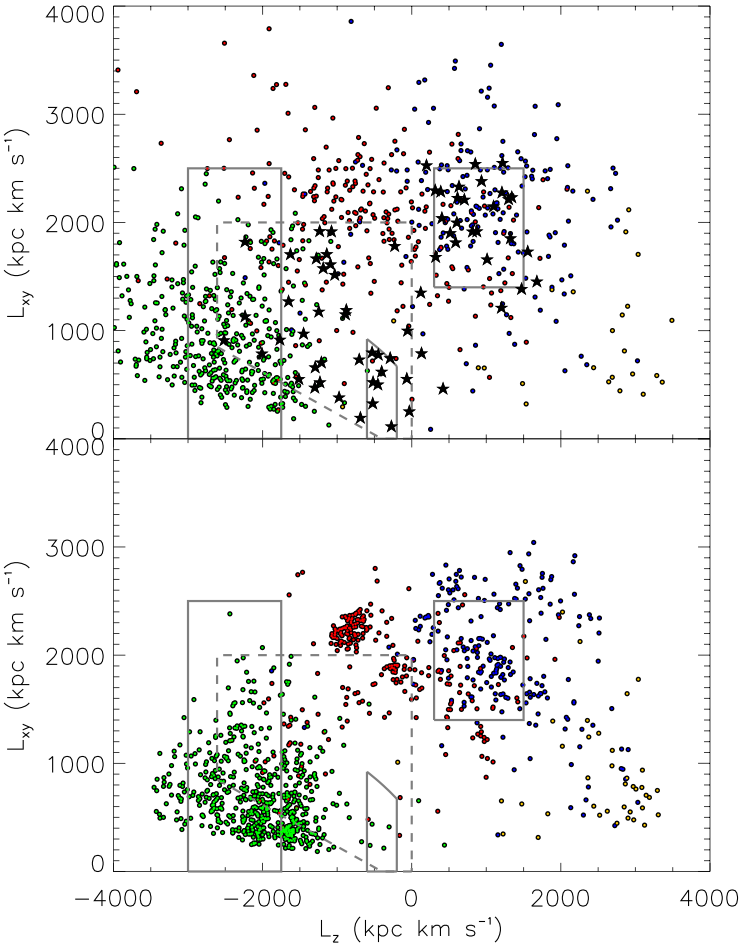
Figure 10.— The $10\%$ high velocity tail component belonging solely to the 4 satellites; convolved with current ground-based errors (top, 835 particles) and with the expected Gaia errors (bottom, 1061 particles). Black star symbols are the $67$ fast moving debris stars uncovered from the analysis of the SGKS sample. Solid and dashed contours have the same meaning as in Figs. 4 and 7 .

7. Conclusions

We have explored the Solar neighborhood of the Milky Way through the use of spectro-photometric data from the Sloan Digital Sky Survey and high-quality proper motions derived from multi-epoch positions extracted from the Guide Star Catalogue II database. A sample with accurate distances, space velocities, and metallicities is selected as a tracer of the inner-halo population resulting in $2417$ subdwarfs with $\rm{[Fe/H]}<-1.5$ and $\rm{|z|>1}$ kpc within $3$ kpc of the Sun. This set is then analysed to identify and characterise kinematic streams possibly arising from merging events.

We have found statistical evidence of substructures in the space motions of the $10\%$ fastest stars, confirming the existence of $5$ moving groups.

In angular momenta space, the two prograde groups we have identified (Groups 1 and 2 in Table 2) appear confined in the region encompassing the stream first identified by Helmi et al. (1999) among red giants and RR Lyrae within $1$ kpc of the Sun. Our analysis found $25$ additional subdwarf members belonging to that same stream: $4$ are in common with those found by Klement et al. (2009), while the other $21$ are newly discovered members.

Of the remaining groups, the most counter-rotating one (Group 4) partially overlaps with the region of “retrograde outliers” found by Kepley et al. (2007), while a dozen stars belonging to Group 4 and Group 5 fall in the region of the mildly retrograde stream detected by Dinescu (2002).

Comparison to our high resolution N-body simulations confirms that the two groups associated with the Helmi stream are likely fossil remnants of a dwarf galaxy which co-rotates with the disk of the Galaxy and moves on a high-inclination orbit.

As for the three retrograde groups (3, 4 and 5 in Table 2), they may be debris of an unique progenitor accreted along an initial retrograde orbit having an intermediate inclination in the range $10^{\circ}\div 60^{\circ}$. However, we cannot exclude that these groups belong to different impacting satellites on retrograde orbits with inclinations within that same range. A more detailed analysis of the chemical abundances of the three detected groups, as well as more quantitative comparisons to extended simulations, are necessary to resolve this issue.

In any event, the fastest objects appear with positive and negative $L_{z}$ values (i.e. prograde and retrograde motions, respectively) in the angular momentum $(L_{z},L_{xy})$ regions for high-inclination orbits ($L_{xy}\gtrsim 1500~{}\rm{kpc~{}km~{}s^{-1}}$). On the other hand, for low-inclination both observations and simulations show that the fastest objects appear only on retrograde orbits (e.g., Fig. 10, top panel). This asymmetric distribution is suggestive of the role played by dynamical friction during accretion.

In anticipation of the much improved data expected over the coming years, in particular the Gaia catalogue and the new ground-based spectroscopic surveys, we also investigated the impact of observational errors in our dynamical simulations. The analysis indicates that (see the relevant panels of Figs. 8 and 10) Gaia will greatly influence these studies: for, velocity and angular momentum distribution will be almost completely dominated by the physics we are trying to recover, i.e., the dynamical history of the merging events.

At that point, full grids (in, e.g., inclination and amount of rotation) of prograde and retrograde high resolution satellite simulations will be required to precisely characterise the debris detected. Then, we will be able to number the merging events for direct comparison with the predictions of the ($\Lambda$)CDM theory and its associated merging paradigm.

In conclusion, the results shown might lead us to claim that the inner halo might have “seen” only two events; however the large uncertainties in the extant data, mostly observational, do not exclude the possibility that the events might be as many as four, and perhaps more given the intrinsic difficulty of our technique to deal with low inclination prograde mergers.

References

- Abadi et al. (2006) Abadi, M. G., Navarro, J. F., & Steinmetz, M. 2006, MNRAS, 365, 747
- Abazajian et al. (2009) Abazajian, K. N., Adelman-McCarthy, J. K., Agüeros, M. A., et al. 2010, ApJS, 182, 543
- Allende Prieto et al. (2008) Allende Prieto, C., Sivarani, T., Beers, T. C., et al. 2008, AJ, 136, 2070
- Byrd et al. (1986) Byrd, G. G., Saarinen, S. & Valtonen, M. J. 1986, MNRAS, 220, 619
- Bullock & Johnston (2005) Bullock, J. S., & Johnston K. V. 2005, ApJ, 635, 931
- Binney & Merrifield (1998) Binney, J., & Merrifield, M. 1998, Galactic Astronomy (Princeton Univ. Press, Princeton)
- Binney & Tremaine (1987) Binney, J., & Tremaine, S. 1987, Galactic Dynamics (Princeton Univ. Press, Princeton)
- Bond et al. (2010) Bond, N. A., Ivezić, Ž., Sesar, B., et al. 2010, ApJ, 716, 1
- Chandrasekar (1943) Chandrasekar, S. 1943, ApJ, 97, 255
- Chiba & Beers (2000) Chiba, M., & Beers, T. C. 2000, AJ, 119, 2843
- Colpi et al. (1999) Colpi, M., Mayer, L., & Governato, F. 1999, ApJ, 525, 720
- Dehnen & Binney (1998) Dehnen, W., & Binney, J. J. 1998, MNRAS, 298, 387
- De Lucia (2012) De Lucia, G. 2012, Astron. Nachr., 333, 460
- Dinescu (2002) Dinescu, D. I. 2002, in: F. van Leeuwen, J. Hughes, & G. Piotto (eds.), Centauri: A Unique Window into Astrophysics, (San Francisco: ASP), Vol. 265, p. 365
- Duffau et al. (2014) Duffau, S., Vivas, K. A., Zinn, R., Mendez, R. A., & Ruiz, M. T. 2014, A&A, 566, 118
- Eggen (1977) Eggen, O. J. 1977, ApJ, 215, 812
- Eggen (1971) Eggen, O. J. 1971, PASP, 83, 285
- Freeman & Bland-Hawthorn (2002) Freeman, K., & Bland-Hawthorn, J. 2002, ARA&A, 40, 487
- Gilmore et al. (2012) Gilmore, G., Randich, S., Asplund, M., et al. 2012, The Messenger, 147, 25
- Girardi et al. (2004) Girardi, L., Grebel, E. K., Odenkirken, M., & Chiosi, C. 2004, A&A, 422, 205
- Gomez et al. (2013) Gomez, F. A., Helmi, A., Cooper, A. P., et al. 2013, MNRAS, 436, 3602
- Gould (2003) Gould, A. 2003, ApJ, 592, L63
- Harding et al. (2001) Harding, P., Morrison, H. L., Olszewski, E. W., et al. 2001, AJ, 122, 1397
- Hastie et al. (2001) Hastie, T., Tibshirani, R., & Friedman, J. 2001, The Elements of Statistical Learning (Springer)
- Helmi et al. (2011) Helmi, A., Cooper, A. P., White, S. D. M., et al. 2011, ApJ, 733, L7
- Helmi (2008) Helmi, A. 2008, A&AR, 15, 145
- Helmi & de Zeeuw (2000) Helmi, A., & de Zeeuw, P. T. 2000, MNRAS, 319, 657
- Helmi et al. (1999) Helmi, A., White, S. D. M., de Zeeuw, P. T., & Zhao, H. S. 1999, Nature, 402, 53
- Helmi & White (1999) Helmi, A., & White, S. D. M. 1999, MNRAS, 307, 495
- Hernquist (1993) Hernquist, L. 1993, ApJS, 86, 389
- Ibata et al. (2003) Ibata, R. A., Irwin, M. J., Lewis, G. F., Ferguson, A. M. N., & Tanvir, N. 2003, MNRAS, 340, 21
- Ibata et al. (1994) Ibata, R. A., Gilmore, G., & Irwin, M. J. 1994, Nature, 370, 194
- Ivezić et al. (2008) Ivezić, Ž., Sesar, B., Jurić, M., et al. 2008, ApJ, 684, 287
- Johnston (1998) Johnston, K. V. 1998, ApJ, 495, 297
- Kaufmann & Rousseeuw (1990) Kaufmann, L., & Rousseeuw, P. J. 1990, Finding Groups in Data (John Wiley & Sons, Inc.)
- Kepley et al. (2007) Kepley, A. A., Morrison, H. L., Helmi, A., et al. 2007, AJ, 134, 1579
- Klement (2010) Klement, R. J. 2010, A&AR, 18, 567
- Klement et al. (2009) Klement, R., Rix, H. -W., Flynn, C., et al. 2009, ApJ, 698, 865
- Lasker et al. (2008) Lasker, B. M., Lattanzi, M. G., McLean, B. J., et al. 2008, AJ, 139, 735
- Lee et al. (2008a) Lee, Y. S., Beers, T. C., Sivarani, T., et al. 2008a, AJ, 136, 2022
- Lee et al. (2008b) Lee, Y. S., Beers, T. C., Sivarani, T., et al. 2008b, AJ, 136, 2050
- Majewski et al. (2012) Majewski, S. R., Nidever, D. L., Smith, V. V., et al. 2012, ApJ, 747, L37
- Majewski et al. (1996) Majewski, S. R., Munn, J. E., & Hawley, S. L. 1996, ApJ, 459, 73
- Meza et al. (2005) Meza, A., Navarro, J. F., Abadi, M. G., & Steinmetz, M. 2005, MNRAS, 359, 93
- Moore et al. (2006) Moore, B., Diemand, J., Madau, P., Zemp, M., & Stadel, J. 2006, MNRAS, 368, 563
- Morrison et al. (2009) Morrison, H. L., Helmi, A., Sun, J., et al. 2009, ApJ, 694, 130
- Munn et al. (2008) Munn, J. A., Monet, D. G., Levine, S. E., et al. 2008, AJ, 136, 895
- Murante et al. (2010) Murante, G., Poglio, E., Curir, A., & Villalobos, A. 2010, ApJ, 716, L115
- Navarrete et al. (2015) Navarrete, C., Chaname, J., Meza, A., et al. 2015, to appear in ApJ
- Navarro, Frenk & White (1997) Navarro, J. F., Frenk, C. S., & White, S. D. M. 1997, ApJ, 490, 493
- Pasetto et al. (2012) Pasetto, S., Grebel, E. K., Zwitter, T., et al. 2012, A&A, 547, A70
- Perryman et al. (2001) Perryman, M. A. C., de Boer, K. S., Gilmore, G., et al. 2001, A&A, 369, 339
- Read et al. (2008) Read, J. I., Lake, G., Agertz, O., & Debattista, V. P. 2008, MNRAS, 389, 1041
- Re Fiorentin et al. (2007) Re Fiorentin, P., Bailer-Jones, C. A. L., Lee, Y. S., et al. 2007, A&A, 467, 1373
- Re Fiorentin et al. (2005) Re Fiorentin, P., Helmi, A., Lattanzi, M. G., & Spagna, A. 2005, A&A, 439, 551
- Sales et al. (2007) Sales, L. V., Navarro, J. F., Abadi, M. G., & Steinmetz, M. 2007, MNRAS, 379, 1464
- Schlaufman et al. (2009) Schlaufman, K.C., Rockosi, C. M., Allende Prieto, C., Beers, T. C., Bizyaev, D., et al. 2009, ApJ, 703, 2177
- Schlaufman et al. (2011) Schlaufman, K.C., Rockosi, C. M., Lee, Y.S., Beers, T.C., & Allende Prieto, C. 2011, ApJ, 734, 49
- Schlafly et al. (2014) Schlafly, E. F., Green, G., Finkbeiner, D. P., et al. 2014, ApJ, 789, 15
- Schlafly & Finkbeiner (2011) Schlafly, E. F., & Finkbeiner, D. P. 2011, ApJ, 737, 103
- Schlegel et al. (1998) Schlegel, D. J., Finkbeiner, D. P., & Davis, M. 1998, ApJ, 500, 525
- Searle & Zinn (1978) Searle, L., & Zinn, R. 1978, ApJ, 225, 357
- Smith et al. (2009) Smith, M. C., Evans, N. W., Belokurov, V., et al. 2009, MNRAS, 399, 1223
- Spagna et al. (2010a) Spagna, A., Lattanzi, M. G., Re Fiorentin, P., & Smart, R. L. 2010a, A&A, 510, L4
- Spagna et al. (2010b) Spagna, A., Bucciarelli, B., Lattanzi, M. G., Re Fiorentin, P., & Smart, R. L. 2010b, MemSAIt, 14, 67
- Spagna et al. (2004) Spagna, A., Carollo, D., Lattanzi, M. G., & Bucciarelli, B. 2004, A&A, 428, 451
- Springel (2005) Springel, V. 2005, MNRAS, 364, 1105
- Starkenburg et al. (2009) Starkenburg, E., Helmi, A., Morrison, H. L., et al. 2009, ApJ, 698, 567
- Trumpler & Weaver (1953) Trumpler R. J., & Weaver H. F. 1953, Statistical Astronomy (Dover Pubblications, Inc., New York)
- Turon et al. (2005) Turon, C., O’Flaherty, K. S., & Perryman, M. A. C. eds. 2005, The Three-dimensional universe with Gaia, ESA Spec. Publ., 576
- Villalobos & Helmi (2008) Villalobos, A., & Helmi, A. 2008, MNRAS, 391, 1806
- Yanny et al. (2009) Yanny, B., Rockosi, C., Newberg, H. J., et al. 2009, AJ, 137, 4377
- Zhao et al. (2012) Zhao, G., Zhao, Y.-H., Chu, Y.-Q., et al. 2012, RAA, 12, 723