Cross-Layer Design of Wireless Multihop Networks over Stochastic Channels with Time-Varying Statistics

Abstract

Network Utility Maximization is often applied for the cross-layer design of wireless networks considering known wireless channels. However, realistic wireless channel capacities are stochastic bearing time-varying statistics, necessitating the redesign and solution of NUM problems to capture such effects. Based on NUM theory we develop a framework for scheduling, routing, congestion and power control in wireless multihop networks that considers stochastic Long or Short Term Fading wireless channels. Specifically, the wireless channel is modeled via stochastic differential equations alleviating several assumptions that exist in state-of-the-art channel modeling within the NUM framework such as the finite number of states or the stationarity. Our consideration of wireless channel modeling leads to a NUM problem formulation that accommodates non-convex and time-varying utilities. We consider both cases of non orthogonal and orthogonal access of users to the medium. In the first case, scheduling is performed via power control, while the latter separates scheduling and power control and the role of power control is to further increase users’ optimal utility by exploiting random reductions of the stochastic channel power loss while also considering energy efficiency. Finally, numerical results evaluate the performance and operation of the proposed approach and study the impact of several involved parameters on convergence.

I Introduction

Network Utility Maximization (NUM) is a very popular tool in the communications research community, for cross-layer design and optimization of wireless networks. Typically, a utility function is assigned to each network flow (source-destination pair), and the sum of all utilities over the network is maximized, subject to network stability constraints. Most approaches in literature applying NUM, consider ideal or stationary and ergodic wireless channels. However, under realistic conditions, fading occurring in wireless channels hampers the performance in wireless communications, leading to stochastic, i.e. time and space varying, random (thus unknown), wireless link capacities possibly bearing time-varying statistics. Therefore, it becomes necessary to reformulate/redesign and solve the basic NUM problem for incorporating realistic stochastic wireless channel conditions by addressing non-stationarity issues, and also transient phenomena occurring when the network operates for a finite time interval.

This paper aims at treating this problem by proposing a novel optimization framework for joint congestion control, routing, scheduling and power control based on NUM, under stochastic possibly non-stationary Long Term Fading (LTF) or Short Term Fading (STF) wireless channels. Congestion control determines the optimal sources’ data production rates, routing determines the optimal routes of the flows within the network, while the set of transmitting links and their corresponding transmission powers are chosen based on scheduling and power control. The proposed optimization framework refers to a finite network operation and it is developed for two cases, where the first one deals with non-orthogonal access to the wireless medium and the second deals with orthogonal access to the wireless medium. In the first case, scheduling is performed via power control, while in the latter case, scheduling and power control are separated. On the one hand, non-orthogonal access leads to a very hard to solve cross terminal power control/scheduling problem in the physical layer. On the other hand, orthogonal access to the medium allows for more efficient and distributed power control in the physical layer, although introducing the need of the NP-hard computation of all the independent sets of the network graph for scheduling. Importantly, in the case of orthogonal access, the role of power control is to further boost link capacity and consequently source rates by exploiting good channel states and to save energy when the channel state is destructive for the transmitted signal.

The structure of the rest of the paper is as follows. Section II presents the related literature while summarizing the basic contributions of this paper. Then, Section III describes the considered STF and LTF channel models derived with the use of stochastic differential equations, while Section IV presents the considered system model. Sections V and VI focus on the analysis and solution of the proposed optimization framework in the cases of non-orthogonal and orthogonal access to the wireless medium respectively. Finally, in Section VII numerical results are presented to evaluate the proposed approach and Section VIII concludes the paper.

II Related Work & Contributions

Several works exist in the literature targeting at incorporating the stochastic wireless channels in the NUM problem’s formulation and solution. In [1], the channel quality is expressed via the SIR (Signal-to-Interference-Ratio), since the latter is affected by interference due to parallel transmissions and LTF. It is assumed that the LTF parameters are deterministic and slowly varying, allowing for the algorithms which perform joint congestion and power control to converge in the meantime of their change. In [2], [3], the case of composite fading (LTF and STF) is examined, considering channel conditions that vary faster than the algorithm’s convergence, via the use of outage-probabilities in the NUM problem formulation. In [2], [3], STF follows Rayleigh and Nakagami distributions respectively, where however the statistics of the distributions remain invariant. A different approach is followed in [4, 5], where NUM is extended to Wireless NUM (WNUM), with random channel conditions. WNUM leads to policies for controlling the network by responding optimally to the change of the channel state, based on random samples without a priori knowledge of the wireless channels’ statistics. Although the statistics of the channel may be unknown, the latter is considered as stationary and ergodic.

In the sequel, in [6], NUM is employed to perform, joint congestion control, power control, routing and scheduling assuming that the channel fading process is stationary and ergodic. Similarly in [7, 8], joint congestion control, routing and scheduling is performed in the framework of NUM while assuming that there is a finite number of channel states. In these works, the network functions in time slots, where during each time slot the channel state remains stable and changes randomly and independently on the boundary of time slots. Finally, in [9] the convergence of primal-dual algorithms for solving NUM is studied under wireless fading channels with time-varying parameters (and thus statistics). Time-varying statistics of wireless channels lead to time-varying optimal solutions of the NUM problem necessitating the study of how well the solution algorithms track the changes in the optimal values. However, it is assumed that the channel fading parameters vary following a Finite State Markov Chain.

In a nutshell, in the existing body of research work in literature, the wireless channel modeling in the framework of NUM is characterized by one or combinations of the following assumptions: (a) The channel process is stationary and ergodic. (b) The statistics of the wireless channel are fixed in time (and known), or vary at slower rate than the one of the network control algorithms’ convergence. (c) The statistics of the channel change according to a Finite State Markov Chain. All previous approaches are not capable of capturing and tracking complex time and space variations in the propagation environment of realistic systems [10]. In [10], wireless channel models for both LTF and STF are introduced based on Stochastic Differential Equations (SDEs) [11] in order to capture higher order dynamics of the wireless channel. In this case the wireless channel is modeled via stochastic processes which may have time-varying statistics. By means of SDEs, it is possible to express an LTF or an STF channel capturing both space and time variations [10], [12], as it will be described in detail in Section III.

In our paper, the NUM problem is reformulated and solved using the SDE model to capture the wireless channel state. Emphasis is placed on LTF especially for demonstration purposes. Due to the possible non-stationarity of the wireless channel we cannot formulate the NUM problem based on the stationary mean values of the involved optimization variables (e.g. [6], [7], [13]). On the contrary we will adopt the stochastic optimal control problem’s formulation [14] based on expected values over time integrals, thus also allowing for the consideration of a finite time duration of the network’s operation. In [15], we proposed a preliminary version of this approach focused on congestion and power control in the case of orthogonal access to the wireless medium. The basic contributions of this paper can be summarized as:

• We develop a framework for the cross-layer design and control of the operation of wireless multihop networks, i.e. for congestion and power control, routing and scheduling, over wireless channels (LTF or STF) that are stochastic but not necessarily stationary.

• The proposed problem formulation adopts a (more realistic) finite duration of the network’s operation (e.g. corresponding to the case of finite battery levels of the wireless nodes or of finite flows) where the wireless channel may still operate in a transient state, even though there may exist a limiting stationary distribution. The extension to an infinite duration of the network’s operation is discussed.

• Utilities are not necessarily convex functions but adopt a more general form (more specifically a continuous differentiable one), contrary to the related papers in literature (e.g. [6], [7], [13]) that assume convex utility forms. This fact is important since it allows for addressing the case of real time traffic modeled, for example, by sigmoidal utilities [16]. Zero duality gap is analytically proven in this case of general utilities, following a technique that leverages from the wireless channels’ continuous stochastic modeling.

• The proposed problem formulation (expected values over time integrals) allows for the adoption of time-varying utility functions. This serves the purpose of evolving users’ preferences/needs and is also aligned with the finite network duration, i.e. nodes may desire to produce significantly less data close to the end of the network operation. To the best of our knowledge, this fact has not been addressed in the literature.

• Power control is shown to further boost link capacity and thus source rates by exploiting good channel conditions while saving energy in case of destructive channel conditions.

• Finally, we prove an interesting theorem in the case of LTF, elucidating a basic advantage with respect to the optimal users’ utilities when exploiting the random channel fluctuations, compared to the conventional NUM problem formulation (e.g. [7], [13]). Specifically, it is proven that, contrary to what is possibly expected, a higher value of the diffusion coefficient of the wireless channels’ power loss leads to higher optimal sum of users’ utilities, fact that cannot be captured by the conventional NUM modeling approach. We also show via numerical evaluations that a higher diffusion coefficient achieves simultaneously a reduced power consumption leading to energy efficiency. This result emphasizes the importance of utilizing a more realistic power loss model such as the one of an SDE, as opposed to the mean power loss model used in the conventional NUM problem formulation.

III Background on Wireless Channel Modeling via SDEs

The objective of this section is to briefly describe the SDE-based LTF and STF channel models, developed in the literature, and their assumptions, upon which, the optimization problems of the following sections will be formulated and solved.

III-A Long Term Fading (LTF)

LTF consists of path loss and shadowing [17]. Path loss is due to the dissipation of the transmitted power and the effects of the propagation channel, while shadowing is caused by obstacles between the transmitter and the receiver. LTF depends on the geographical area and occurs in sparsely populated or suburban areas. Before describing the dynamic in time LTF model for the wireless channels [10], we recall the conventional LTF model, where the power loss $PL$ along a given link $(i,j)$ between nodes $i$ and $j$ in Euclidean distance $d_{ij}$, is given [17]:

$$PL(d_{ij})[dB]=\overline{PL}(d_{0})[dB]+10\gamma\log\big{(}\frac{d_{ij}}{d_{0}}\big{)}+\tilde{Z},~{}d_{ij}\geq d_{0},$$ (1)

where $\gamma$ is the power loss exponent and depends on the wireless propagation medium, $d_{0}$ is the reference distance, $\overline{PL}(d_{0})$ is the expected power loss on the reference distance, and $\tilde{Z}\sim\mathcal{N}(0;\sigma^{2})$, is a gaussian random variable with zero mean and variance $\sigma^{2}$, used to model any uncertainty in the propagation environment. Note that the statistics (mean (denoted as $\overline{PL}(d_{ij})$) and variance) of the conventional LTF model are invariant in time.

In the following, we describe the extension of the LTF model to dynamically changing conditions in time, as it is developed in [10]. Specifically, the random variable, $PL(d_{ij})[dB]$, of Eq. (1), becomes a stochastic process denoted as $\{X_{ij}(t)\}_{t\geq t_{0}}$ ([dB]), where $t$ represents time. Time dependence is used to capture time variations of the propagation environment due to e.g. movement of objects and scatterers in the area surrounding the network. In a similar spirit with Eq. (1), $\{X_{ij}(t)\}_{t\geq t_{0}}$, represents the power lost by the signal during a transmission from $i$ to $j$ at a particular distance $d_{ij}$. Although, $\{X_{ij}(t)\}_{t\geq t_{0}}$ depends on the distance $d_{ij}$, we do not explicitly model this dependence as the network considered is static.

In [10], $\{X_{ij}(t)\}_{t\geq t_{0}}$, $\forall(i,j)$, are modeled as solutions of mean reverting linear SDEs, given as:

$$dX_{ij}(t)=\beta_{ij}(t)\big{(}\gamma_{ij}(t)-X_{ij}(t)\big{)}dt+\delta_{ij}(t)dW_{ij}(t),~{}X_{ij}(t_{0})\sim\mathcal{N}(\overline{PL}(d_{ij})[dB];\sigma^{2}),$$ (2)

where $\{W_{ij}(t)\}_{t\geq t_{0}}$, $\forall(i,j)$, are independent standard Brownian motions defined over a filtered probability space $(\Omega,\mathcal{F},\{\mathcal{F}_{t}\}_{t\geq t_{0}},\mathbf{P})$ and each one being independent of the corresponding $X_{ij}(t_{0})$. $\{\mathcal{F}_{t}\}_{t\geq t_{0}}$ is the filtration produced by $X_{ij}(t_{0})$, $\forall(i,j)$, and the Brownian motions themselves. For each $(i,j)$, $\gamma_{ij}(t)$ is the power loss level $X_{ij}(t)$ is attracted to, $\beta_{ij}(t)$ is the positive speed of this adjustment and finally, $\delta_{ij}(t)$ is the diffusion coefficient of the SDE, determining the “noise” of the channel. The parameters $\beta_{ij}(t),\gamma_{ij}(t),\delta_{ij}(t)$, $\forall(i,j)$, are assumed to be deterministic and can be estimated directly from signal measurements following the approaches in [26], [18], [19], which can be implemented online, i.e. while receiving the signal measurements. The existence of a strong solution to the SDE (2) is satisfied if the relation $\int\limits_{s}^{T}\left\{\beta_{ij}(t)\left|\gamma_{ij}(t)\right|+\delta_{ij}^{2}(t)\right\}dt<\infty,\forall(i,j)$ holds [11]. The time dependent attenuation coefficient (in squared magnitude) equals to: $a_{ij}(t)=e^{-\frac{\ln 10}{10}X_{ij}(t)}=e^{KX_{ij}(t)},~{}\forall(i,j),~{}K=-\frac{\ln 10}{10}$. In [10], it is shown that when all the parameters of the SDE (2) are time independent, its solution tends to the conventional LTF model (Eq. (1)) as $t\rightarrow\infty$ (which is stationary). In general when the parameters of the SDE (2) change with time, $X_{ij}(t)$ is gaussian with time-varying statistics and a stationary distribution may not exist.

III-B Short Term Fading (STF)

In a similar spirit as LTF, in [12], [18], [10] a stochastic model for STF wireless channels has been developed, alleviating the assumption of stationarity. This kind of signal fading is due to the constructive and destructive addition of multipath components [17] created from reflections, diffractions and scattering and usually occurring in densely built-up areas. The statistics of the STF models usually applied in the literature (e.g. Rayleigh, Nakagami, Ricean, etc. [2], [17]), are assumed constant over local areas (i.e. at a microscopic level) [12]. However, STF wireless channels are of stochastic nature with time varying statistics mainly due to the continuous and arbitrary change of the propagation environment if the transmitter, the receiver or objects between them move. The latter is the main reason why in this paper, we adopt a stochastic process with time varying statistics for modeling STF channels.

For the models developed in [12], [18], the inphase and quadrature components of the wireless fading channels are assumed conditionally uncorrelated gaussian random variables (thus conditionally independent). In the case of flat fading, the multipath components are not resolvable and can be considered as a single path. Then, the inphase, $I$, and quadrature, $Q$, components over one link (e.g. $(i,j)$) can be realized as:

$$dX_{I}(t)=A_{I}(t)X_{I}(t)dt+B_{I}(t)dW_{I}(t),~{}X_{I}(t_{0}),~{}I(t)=C_{I}X_{I}(t),$$

$$dX_{Q}(t)=A_{Q}(t)X_{Q}(t)dt+B_{Q}(t)dW_{Q}(t),~{}X_{Q}(t_{0}),~{}Q(t)=C_{Q}X_{Q}(t),$$

where $X_{I}(t),~{}X_{Q}(t)$ are the state vectors of the inphase and quadrature components and $\{W_{I}(t)\}_{t\geq t_{0}}$, $\{W_{Q}(t)\}_{t\geq t_{0}}$ are independent standard Brownian motions corresponding to the inphase and the quadrature components respectively, defined over a filtered probability space $(\Omega,\mathcal{F},\{\mathcal{F}_{t}\}_{t\geq t_{0}},\mathbf{P})$. The same model describes every link with different parameter values $A_{I}(t),~{}A_{Q}(t)$, $B_{I}(t)$, $B_{Q}(t)$, $C_{I},~{}C_{Q}$ and (independent) Brownian motions $W_{I}(t),~{}W_{Q}(t)$, but this fact is not explicitly modeled for ease of presentation. The attenuation coefficient (in squared magnitude) is [19] $a_{ij}(t)=I(t)^{2}+Q(t)^{2}.$ As in the case of LTF, the coefficients $A_{I}(t),~{}A_{Q}(t),~{}B_{I}(t),~{}B_{Q}(t),~{}C_{I},~{}C_{Q}$ can be obtained directly via signal measurements following the methodology proposed in [19], [18] using the EM algorithm together with Kalman filtering. This model leads to time-varying mean and variance for the inphase and the quadrature components and thus for the STF wireless channel and includes the Ricean, Rayleigh and Nakagami distributions as special cases [12].

In the rest of the paper, the vectors $X(t),~{}W(t)$ denote collectively (for all links) the channel states and the Brownian motions respectively at time $t$. Note that we assume that the wireless channels are uncorrelated. This assumption is also made in [20], where it is argued that inter-link correlations do not impact the network capacity region and therefore the maximum utility.

IV System Model & Assumptions

We consider a static wireless multihop network with $N$ nodes and $E$ directed links forming the set $\mathcal{E}$. The network serves $F$ overlaying flows (source-destination pairs) over a finite duration (lifetime) $[s,T]$. At time $t\in[s,T]$, $\lambda_{i}^{d}(t)$ data (e.g. packets) are produced from the source node $i$ for its destination node $d$. Let $S_{r}(d)$ be the set of sources for node $d$. Then, $\lambda_{i}^{d}(t)=0,~{}\forall i\notin S_{r}(d),~{}\forall t\in[s,T]$. We denote with $r_{ij}^{d}(t)$ the communication traffic on the link $(i,j)$ for destination $d$ at time $t\in[s,T]$. Then, $R(t),~{}\Lambda(t),$ denote collectively the variables $\{r_{ij}^{d}(t)\}_{\forall d,(ij)},~{}\{\lambda_{i}^{d}(t)\}_{\forall i,d},$ respectively, at time $t$. The set $\mathcal{R}(i,d)$ consists of the one-hop (out-)neighbors of node $i$ which are allowed to serve as next-hop nodes towards $d$ according to the routing protocol under consideration. If there are no routing constraints, we consider $\mathcal{R}(i,d)=\mathcal{N}^{out}(i)$, where $\mathcal{N}^{out}(i)=\{j|(i,j)\in\mathcal{E}\}$. Also, $r_{ij}^{d}(t)=0$, if $j\notin\mathcal{R}(i,d)$ and $r_{ii}^{d}(t)=0,~{}r_{di}^{d}(t)=0,~{}\forall i,d,t\in[s,T]$. Furthermore, we assume that the transmitter of the link $(i,j)$, i.e. the node $i$, transmits with power $P_{ij}(t)$ at time $t\in[s,T]$. $P(t)$ expresses collectively the transmission powers of all links at time $t\in[s,T]$.

Each source node associates its satisfaction for its produced data for destination $d$, $\lambda_{i}^{d}$, at time $t\in[s,T]$, with a time-varying continuous differentiable utility function $U_{i}^{d}(\lambda_{i}^{d},t)$. Several utility functions used in literature belong in this category, such as the strictly convex and increasing $a$-fair utility, including the logarithmic one [21]. It is further assumed that $U_{i}^{d}(\lambda_{i}^{d},t)$ is increasing with $\lambda_{i}^{d}$ and uniformly bounded as $t\rightarrow\infty$. Also, a (continuous differentiable) cost function, $J_{ij}(P_{ij})$, is assigned to each directed link $(i,j)$ with respect to its transmission power $P_{ij}(t)$, $t\in[s,T]$. In literature, $J_{ij}(P_{ij})$ is often assumed to be a strictly convex function [6].

The proposed cross-layer framework includes routing, scheduling, power and congestion control. Routing (network layer) determines the amount of traffic for each destination that will be served by every link, by optimizing $R(t)$, $\forall t\in[s,T]$. Scheduling and power control (MAC and physical layers) determine which links are going to transmit and their transmission power by optimizing $P(t)$, $\forall t\in[s,T]$. Finally, congestion control (transport layer) optimizes $\Lambda(t)$, $\forall t\in[s,T]$. Therefore, the proposed cross-layer scheme aims at determining the optimal values of the control variables $R(t),~{}\Lambda(t),~{}P(t)$, $\forall t\in[s,T]$, according to an optimality criterion designed with the aid of the utility and cost functions defined above, considering the channel models of Section III.

Due to the considered underlying channel processes, the control variables $R,~{}\Lambda,~{}P$ should be in general defined as stochastic processes. Let us define the value range for each $\lambda_{i}^{d}$, $U_{\lambda}=[0,\lambda_{\max}]$, and the corresponding feasible set $\mathcal{U}_{\lambda}=\left\{\lambda:[s,T]\times\Omega\rightarrow U_{\lambda}:\lambda\mathrm{~{}is~{}}\{\mathcal{F}_{t}\}_{t\geq s}\mathrm{~{}adapted}\right\}$. Then, $\Lambda\in\mathcal{U}_{\lambda}^{F}$. Similarly, we define the value range for each $r_{ij}^{d}$, $U_{r}=[0,R_{\max}]$, and the corresponding feasible set $\mathcal{U}_{r}=\left\{r:[s,T]\times\Omega\rightarrow U_{r}:r\mathrm{~{}is~{}}\{\mathcal{F}_{t}\}_{t\geq s}\mathrm{~{}adapted}\right\}$. Then, $R\in\mathcal{U}_{r}^{E\times(N-1)}$. Finally, we define the value range for each $P_{ij}$, $U_{P}=[0,P_{\max}]$, and the corresponding feasible set $\mathcal{U}_{P}=\left\{P:[s,T]\times\Omega\rightarrow U_{P}:P\mathrm{~{}is~{}}\{\mathcal{F}_{t}\}_{t\geq s}\mathrm{~{}adapted}\right\}$. Then, $P\in\mathcal{U}_{P}^{E}$. We will use $\mathbb{E}_{s,x}$ to denote expectations given the initial condition $X(s)=x$.

At this point, we distinguish two cases with respect to the access to the wireless medium. Based on the two types of access, two cross-layer problems are developed. The first case concerns non-orthogonal access to the wireless medium, in which the transmitters are allowed to access the wireless medium simultaneously (one frequency carrier is assumed), while the interfering transmissions are considered as noise. For this case we define the Signal-to-Interference-plus-Noise-Ratio $(SINR)$ for the link $(i,j)$ as follows: $SINR_{ij}(t)=\frac{a_{ij}(t)P_{ij}(t)}{N_{0}+\sum_{(k,l)\in\mathcal{I}_{ij}}a_{kj}P_{kl}(t)}$, where $\mathcal{I}_{ij}$ denotes the subset of $\mathcal{E}$ containing the links that interfere with the link $(i,j)$. $N_{0}$ (Watts) stands for the average background noise at the receiver’s ($j$) side and $a_{ij}(t)$ is defined in Section III depending on the fading type. The capacity of the link $(i,j)$ is given by the Shannon’s formula in bits/sec as $C_{ij}(P(t))=B_{ij}\log_{2}(1+SINR_{ij}(t))$, where $B_{ij}$ ($Hertz$) is the wireless channel’s bandwidth at link $(i,j)$. The second case refers to the orthogonal access to the wireless medium, where only non-interfering links can access simultaneously the wireless medium. Orthogonal access decreases the complexity of the proposed framework’s operation in the physical layer (power control), as it will be shown in later sections, while it is nearly optimal when interference is strong [6]. In this case, the connectivity graph of the wireless multihop network is important in identifying the feasible schedules. Based on the latter, the finite set of all possible independent sets of links (i.e. links that do not interfere with each other) is constructed. Only links belonging to the same independent set can access the wireless medium simultaneously. In this case, the capacity of the link $(i,j)$ is a concave function of $P_{ij}$, given in bits/sec as $C_{ij}(P_{ij}(t))=B_{ij}\log_{2}\left(1+\frac{a_{ij}(t)P_{ij}(t)}{N_{0}}\right)$.

V Non-orthogonal Access to the Medium

V-A Problem Formulation & Analysis

According to the discussion in Section IV, the optimization framework, denoted as $\mathbf{P_{1}}$, is formulated as follows.

$$P_{1}:=\max_{\Lambda\in\mathcal{U}_{\lambda}^{F},~{}R\in\mathcal{U}_{r}^{E\times(N-1)},~{}P\in\mathcal{U}_{P}^{E}}\mathbb{E}_{s,x}\left[\int_{s}^{T}\left(\sum_{i,d:i\in S_{r}(d)}U_{i}^{d}(\lambda_{i}^{d}(t),t)-\sum_{(i,j)}J_{ij}(P_{ij}(t))\right)dt\right]$$

$$s.t.$$

$$\mathbb{E}_{s,x}\left[\int_{s}^{T}\lambda_{i}^{d}(t)dt+\int_{s}^{T}\sum_{j:i\in\mathcal{R}(j,d)}r_{ji}^{d}(t)dt\right]\leq\mathbb{E}_{s,x}\left[\int_{s}^{T}\sum_{j\in\mathcal{R}(i,d)}r_{ij}^{d}(t)dt\right],~{}\forall i,d$$ (3)

$$\mathbb{E}_{s,x}\left[\int_{s}^{T}\sum_{d}r_{ij}^{d}(t)dt\right]\leq\mathbb{E}_{s,x}\left[\int_{s}^{T}C_{ij}(P(t))dt\right],~{}\forall(i,j)\in\mathcal{E}$$ (4)

$$\mathbb{E}_{s,x}\left[\int_{s}^{T}\sum_{j\in\mathcal{N}^{out}_{i}}P_{ij}(t)dt\right]\leq P_{i,\max},~{}\forall i$$ (5)

The objective function expresses the trade-off between the accumulated for all sources utilities/satisfaction of producing data and the accumulated cost due to power consumption for link transmissions. Thus, its maximization targets at improving energy efficiency by maximizing source rates while penalizing the cost of power consumption for achieving them when $J_{ij}\neq 0,~{}\forall(i,j)$, i.e. when power control is applied. The first constraint relates to the flow conservation at each node and for each destination, used to ensure high throughput for the examined time interval $[s,T]$. The second constraint relates to the capacity restriction (right side) due to power, channel and interference limitations for each link. Finally, the third constraint, relates to a limitation on the total power consumption of each node for the examined time interval, $[s,T]$, (left side) according to its energy storage, denoted as $P_{i,\max}>0$ (right side).

It is important to note that we consider continuous time network operation (thus, using time integrals), for ease of presentation, due to the continuous time evolution of the channel state (Section III). The case of discrete time network operation can be obtained trivially by replacing the integrals $\int_{s}^{T}$ by sums $\sum_{t=0}^{t=N_{L}}$ where $N_{L}$ is the number of time slots in $[s,T]$ considered for the network operation and each denoted by $t$. In this case the channel state will be sampled at each time slot as described in the subsequent sections. Furthermore, for considering an infinite $T$, we should also divide every integral by $T$, thus considering time averages.

This problem is non-convex due to the forms of the capacity, utility and cost functions. Even if the utility and cost functions were concave and convex respectively as commonly assumed in literature, the problem would still be non-convex due to the capacity function forms. However, we will prove that its duality gap is zero, which is an important fact as it renders the Lagrange (dual)-based optimization method optimal. The latter allows for devising efficient algorithmic solutions as it leads to a separable optimization problem with respect to the variables of each layer while using the Lagrange multipliers for the communication between adjacent layers for achieving a cross-layer optimal solution. Let $\mu_{i}^{d}\geq 0,~{}\forall i,d,~{}l_{ij}\geq 0,~{}\forall(i,j)\in\mathcal{E},~{}\nu_{i}\geq 0,~{}\forall_{i}$ be the Lagrange multipliers associated with the constraints (3), (4), (5) correspondingly. Denote with $L$ the whole set of the Lagrange multipliers. Then, the dual function is formulated as follows:

$$L_{A}(L)=\max_{\Lambda\in\mathcal{U}_{\lambda}^{F},~{}R\in\mathcal{U}_{r}^{E\times(N-1)},~{}P\in\mathcal{U}_{P}^{E}}~{}\mathbb{E}_{s,x}\left[\int_{s}^{T}\left(\sum_{i,d:i\in S_{r}(d)}U_{i}^{d}(\lambda_{i}^{d}(t),t)-\sum_{(i,j)}J_{ij}(P_{ij}(t))\right)dt\right]$$

$$-\sum_{i,d}\mu_{i}^{d}\mathbb{E}_{s,x}\left[\int_{s}^{T}\lambda_{i}^{d}(t)dt+\int_{s}^{T}\sum_{j:i\in\mathcal{R}(j,d)}r_{ji}^{d}(t)dt-\int_{s}^{T}\sum_{j\in\mathcal{R}(i,d)}r_{ij}^{d}(t)dt\right]$$

$$-\sum_{(i,j)\in\mathcal{E}}l_{ij}\mathbb{E}_{s,x}\left[\int_{s}^{T}\sum_{d}r_{ij}^{d}(t)dt-\int_{s}^{T}C_{ij}(P(t))dt\right]-\sum_{i}\nu_{i}\mathbb{E}_{s,x}\left[\int_{s}^{T}\sum_{j\in\mathcal{N}^{out}_{i}}P_{ij}(t)dt-P_{i,\max}\right].$$ (6)

Consequently, the dual problem of $P_{1}$ is defined as $D_{1}:=\inf_{L}(L_{A}(L))$.

Theorem 1

The problem $P_{1}$ has zero dual gap, i.e. if $P_{1}^{*}$ its optimal value and $D_{1}^{*}$ the optimal value of the dual problem, then $P_{1}^{*}=D_{1}^{*}$.

To prove this theorem we proceed in analogy with Theorem $1$ in [22]. The proof relies on the fact that the channel’s cumulative distribution function (cdf) is continuous and thus no channel realization has strictly positive probability. It uses the definition of nonatomic measures and the Lyapunov’s convexity theorem [22].

Proof:

To prove the zero duality gap, we consider a perturbed version of the problem $P_{1}$, obtained by perturbing the constraints used to define the Lagrangian. Let $P_{1}(\Delta)$ be the function that assigns to each perturbation set $\Delta=(\{\Delta_{i,d}^{1}\}_{\forall i,d},\{\Delta_{i,j}^{2}\}_{\forall(i,j)},\{\Delta_{i}^{3}\}_{\forall i})$, the solution of the following perturbed optimization problem.

$$P_{1}(\Delta)=\max_{\Lambda\in\mathcal{U}_{\lambda}^{F},~{}R\in\mathcal{U}_{r}^{E\times(N-1)},~{}P\in\mathcal{U}_{P}^{E}}\mathbb{E}_{s,x}\left[\int_{s}^{T}\left(\sum_{i,d:i\in S_{r}(d)}U_{i}^{d}(\lambda_{i}^{d}(t),t)-\sum_{(i,j)}J_{ij}(P_{ij}(t))\right)dt\right]$$

$$s.t.$$

$$\mathbb{E}_{s,x}\left[\int_{s}^{T}\lambda_{i}^{d}(t)dt+\int_{s}^{T}\sum_{j:i\in\mathcal{R}(j,d)}r_{ji}^{d}(t)dt-\int_{s}^{T}\sum_{j\in\mathcal{R}(i,d)}r_{ij}^{d}(t)dt\right]\leq\Delta_{i,d}^{1},~{}\forall i,d$$ (7)

$$\mathbb{E}_{s,x}\left[\int_{s}^{T}\left(\sum_{d}r_{ij}^{d}(t)-C_{ij}(P(t))\right)dt\right]\leq\Delta_{i,j}^{2},~{}\forall(i,j)\in\mathcal{E},~{}~{}\mathbb{E}_{s,x}\left[\int_{s}^{T}\sum_{j\in\mathcal{N}^{out}_{i}}P_{ij}(t)dt\right]-P_{i,\max}\leq\Delta_{i}^{3},~{}\forall i$$ (8)

i.e. the constraints can be violated by $\Delta$ amounts. In order to prove zero duality gap, we should show that the function $P_{1}(\Delta)$ is a concave function of $\Delta$ [22].

Let $\underline{\Delta}=(\{\underline{\Delta}_{i,d}^{1}\}_{\forall i,d},\{\underline{\Delta}_{i,j}^{2}\}_{\forall(i,j)},\{\underline{\Delta}_{i}^{3}\}_{\forall i})$, $\overline{\Delta}=(\{\overline{\Delta}_{i,d}^{1}\}_{\forall i,d},\{\overline{\Delta}_{i,j}^{2}\}_{\forall(i,j)},\{\overline{\Delta}_{i}^{3}\}_{\forall i})$ be two arbitrary sets of perturbations with respective optimal values $\underline{P_{1}}=P_{1}(\underline{\Delta})$, $\overline{P_{1}}=P_{1}(\overline{\Delta})$ and respective solutions $(\underline{\Lambda},\underline{R},\underline{P})$ and $(\overline{\Lambda},\overline{R},\overline{P})$. Then, for an arbitrary $a\in[0,1]$, we define the perturbation $\hat{\Delta}=a\underline{\Delta}+(1-a)\overline{\Delta}$ and for feasible solutions $(\hat{\Lambda},\hat{R},\hat{P})$, i.e. satisfying the constraints (7), (8), we need to show

$$P_{1}(\hat{\Delta})=P_{1}(a\underline{\Delta}+(1-a)\overline{\Delta})\geq aP_{1}(\underline{\Delta})+(1-a)P_{1}(\overline{\Delta}).$$ (9)

Consider the set of all possible state ($X$) realizations $\mathcal{H}$ and the Borel field, $\mathbb{B}$, on $\mathcal{H}$. For $A\in\mathbb{B}$, let $\mathbb{E}_{s,x}^{A}$ be the expected value restricted on channel realizations included in $A$. We define the following measures.

$$\theta_{id}(A)=\left[\mathbb{E}_{s,x}^{A}\left[\int_{s}^{T}U_{i}^{d}(\underline{\lambda}_{i}^{d}(t),t)dt\right],\mathbb{E}_{s,x}^{A}\left[\int_{s}^{T}U_{i}^{d}(\overline{\lambda}_{i}^{d}(t),t)dt\right]\right],~{}\forall i,d:i\in S_{r}(d),$$ (10)

$$\phi_{id}(A)=\left[\mathbb{E}_{s,x}^{A}\left[\int_{s}^{T}\underline{\lambda}_{i}^{d}(t)dt\right],\mathbb{E}_{s,x}^{A}\left[\int_{s}^{T}\overline{\lambda}_{i}^{d}(t)dt\right]\right],~{}\forall i,d,$$ (11)

$$w_{ij}(A)=\left[\mathbb{E}_{s,x}^{A}\left[\int_{s}^{T}C_{ij}(\underline{P}(t))dt\right],\mathbb{E}_{s,x}^{A}\left[\int_{s}^{T}C_{ij}(\overline{P}(t))dt\right]\right],~{}\forall(i,j)\in\mathcal{E},$$ (12)

$$v_{ij}(A)=\left[\mathbb{E}_{s,x}^{A}\left[\int_{s}^{T}J_{ij}(\underline{P}_{ij}(t))dt\right],\mathbb{E}_{s,x}^{A}\left[\int_{s}^{T}J_{ij}(\overline{P}_{ij}(t))dt\right]\right],~{}\forall(i,j)\in\mathcal{E},$$ (13)

$$\xi_{ij}(A)=\left[\mathbb{E}_{s,x}^{A}\left[\int_{s}^{T}\underline{P}_{ij}(t)dt\right],\mathbb{E}_{s,x}^{A}\left[\int_{s}^{T}\overline{P}_{ij}(t)dt\right]\right],~{}\forall(i,j)\in\mathcal{E},$$ (14)

while we also define $\theta_{id}(\varnothing)=\phi_{id}(\varnothing)=w_{ij}(\varnothing)=v_{ij}(\varnothing)=\xi_{ij}(\varnothing)=0$. These measures are nonatomic [22] since the channel cdf is continuous and all the control variables are bounded. Thus, there are no channel realizations with positive measure, i.e., $\theta_{id}(A)=\phi_{id}(A)=w_{ij}(A)=v_{ij}(A)=\xi_{ij}(A)=0$ for all singleton sets $A\in\mathcal{H}$. Let $W(A)$ be the vector measure expressing collectively all measures $\theta_{id},\phi_{id},w_{ij},v_{ij},\xi_{ij}$, which is also obviously nonatomic. Then from Lyapunov’s convexity theorem [22], the range of $W$ is convex. Therefore, the value $w_{0}=aW(\mathcal{H})+(1-a)W(\varnothing)=aW(\mathcal{H})$ belongs to the range of values of $W$. As a result there exists $A_{0}\in\mathbb{B}$ such that $W(A_{0})=aW(\mathcal{H})$, i.e., $\theta_{id}(A_{0})=a\theta_{id}(\mathcal{H}),~{}\phi_{id}(A_{0})=a\phi_{id}(\mathcal{H})$, etc. Moreover, due to the additivity of measures, for the complement of $A_{0}$, $A_{0}^{c}$, we have $W(A_{0}^{c})=W(\mathcal{H})-W(A_{0})=(1-a)W(\mathcal{H})$. Then, we define the following controls for the new perturbation $\hat{\Delta}$.

$$\hat{r}_{ij}^{d}(t)=a\underline{r}_{ij}^{d}(t)+(1-a)\overline{r}_{ij}^{d}(t),~{}\forall d,(i,j)\in\mathcal{E},t\in[s,T],~{}\mathbf{P}-a.s.$$ (15)

$$\hat{\lambda}_{i}^{d}(t)=\begin{cases}\underline{\lambda}_{i}^{d}(t)~{}\text{within}~{}A_{0}\\ \overline{\lambda}_{i}^{d}(t)~{}\text{within}~{}A_{0}^{c}\end{cases}$$

$$\hat{P}_{ij}(t)=\begin{cases}\underline{P}_{ij}(t)~{}\text{within}~{}A_{0}\\ \overline{P}_{ij}(t)~{}\text{within}~{}A_{0}^{c}\end{cases}\forall i,d:i\in S_{r}(d),\forall(i,j)\in\mathcal{E},t\in[s,T],~{}\mathbf{P}-a.s.$$

Obviously since $\underline{\Lambda},~{}\overline{\Lambda}~{}\in\mathcal{U}_{\lambda}^{F},~{}\underline{R},~{}\overline{R}~{}\in\mathcal{U}_{r}^{E\times(N-1)},~{}\underline{P},~{}\overline{P}~{}\in\mathcal{U}_{P}^{E}$, it also holds that $\hat{\Lambda}\in\mathcal{U}_{\lambda}^{F},~{}\hat{R}\in\mathcal{U}_{r}^{E\times(N-1)},~{}\hat{P}\in\mathcal{U}_{P}^{E}$. Now, based on the above, we check if the controls defined above for the perturbation $\hat{\Delta}$ satisfy Ineqs. (7), (8) and if Ineq. (9) holds. For the constraint (7), we have:

$$\mathbb{E}_{s,x}\left[\int_{s}^{T}\left(\hat{\lambda}_{i}^{d}(t)+\sum_{j:i\in\mathcal{R}(j,d)}\hat{r}_{ji}^{d}(t)-\sum_{j\in\mathcal{R}(i,d)}\hat{r}_{ij}^{d}(t)\right)dt\right]=\mathbb{E}_{s,x}^{A_{0}}\left[\int_{s}^{T}\underline{\lambda}_{i}^{d}(t)dt\right]+\mathbb{E}_{s,x}^{A_{0}^{c}}\left[\int_{s}^{T}\overline{\lambda}_{i}^{d}(t)dt\right]+$$

$$+\mathbb{E}_{s,x}\left[\int_{s}^{T}\sum_{j:i\in\mathcal{R}(j,d)}\left(a\underline{r}_{ji}^{d}(t)+(1-a)\overline{r}_{ji}^{d}(t)\right)dt-\int_{s}^{T}\sum_{j\in\mathcal{R}(i,d)}\left(a\underline{r}_{ij}^{d}(t)+(1-a)\overline{r}_{ij}^{d}(t)\right)dt\right]=$$

$$a\mathbb{E}_{s,x}\left[\int_{s}^{T}\underline{\lambda}_{i}^{d}(t)dt+\int_{s}^{T}\sum_{j:i\in\mathcal{R}(j,d)}\underline{r}_{ji}^{d}(t)dt-\int_{s}^{T}\sum_{j\in\mathcal{R}(i,d)}\underline{r}_{ij}^{d}(t)dt\right]$$

$$+(1-a)\mathbb{E}_{s,x}\left[\int_{s}^{T}\overline{\lambda}_{i}^{d}(t)dt+\int_{s}^{T}\sum_{j:i\in\mathcal{R}(j,d)}\overline{r}_{ji}^{d}(t)dt-\int_{s}^{T}\sum_{j\in\mathcal{R}(i,d)}\overline{r}_{ij}^{d}(t)dt\right]\leq a\underline{\Delta}_{i,d}^{1}+(1-a)\overline{\Delta}_{i,d}^{1}=\hat{\Delta}_{i,d}^{1}.$$ (16)

With respect to the first constraint in (8), we have:

$$\mathbb{E}_{s,x}\left[\int_{s}^{T}\sum_{d}\hat{r}_{ij}^{d}(t)dt\right]-\mathbb{E}_{s,x}\left[\int_{s}^{T}C_{ij}(\hat{P}(t))dt\right]=a\mathbb{E}_{s,x}\left[\int_{s}^{T}\sum_{d}\underline{r}_{ij}^{d}(t)dt-\int_{s}^{T}C_{ij}(\underline{P}(t))dt\right]$$

$$+(1-a)\mathbb{E}_{s,x}\left[\int_{s}^{T}\sum_{d}\overline{r}_{ij}^{d}(t)dt-\int_{s}^{T}C_{ij}(\overline{P}(t))dt\right]\leq a\underline{\Delta}_{i,j}^{2}+(1-a)\overline{\Delta}_{i,j}^{2}=\hat{\Delta}_{i,j}^{2}.$$ (17)

Similarly, with respect to the second constraint in (8), we have:

$$\mathbb{E}_{s,x}\left[\int_{s}^{T}\sum_{j\in\mathcal{N}^{out}_{i}}\hat{P}_{ij}(t)dt\right]-P_{i,\max}=\mathbb{E}_{s,x}^{A_{0}}\left[\int_{s}^{T}\sum_{j\in\mathcal{N}^{out}_{i}}\underline{P}_{ij}(t)dt\right]+\mathbb{E}_{s,x}^{A_{0}^{c}}\left[\int_{s}^{T}\sum_{j\in\mathcal{N}^{out}_{i}}\overline{P}_{ij}(t)dt\right]-P_{i,\max}=$$

$$a\mathbb{E}_{s,x}\left[\int_{s}^{T}\sum_{j\in\mathcal{N}^{out}_{i}}\underline{P}_{ij}(t)dt\right]+(1-a)\mathbb{E}_{s,x}\left[\int_{s}^{T}\sum_{j\in\mathcal{N}^{out}_{i}}\overline{P}_{ij}(t)dt\right]-P_{i,\max}\leq a\underline{\Delta}_{i}^{3}+(1-a)\overline{\Delta}_{i}^{3}=\hat{\Delta}_{i}^{3}.$$ (18)

Finally, $P_{1}(\hat{\Delta})\geq\mathbb{E}_{s,x}\left[\int_{s}^{T}\left(\sum_{i,d:i\in S_{r}(d)}U_{i}^{d}(\hat{\lambda}_{i}^{d}(t),t)-\sum_{(i,j)}J_{ij}(\hat{P}_{ij}(t))\right)dt\right]$, i.e.,

$$P_{1}(\hat{\Delta})\geq=\mathbb{E}_{s,x}^{A_{0}}\left[\int_{s}^{T}\left(\sum_{i,d:i\in S_{r}(d)}U_{i}^{d}(\underline{\lambda}_{i}^{d}(t),t)-\sum_{(i,j)}J_{ij}(\underline{P}_{ij}(t))\right)dt\right]$$

$$+\mathbb{E}_{s,x}^{A_{0}^{c}}\left[\int_{s}^{T}\left(\sum_{i,d:i\in S_{r}(d)}U_{i}^{d}(\overline{\lambda}_{i}^{d}(t),t)-\sum_{(i,j)}J_{ij}(\overline{P}_{ij}(t))\right)dt\right]=aP_{1}(\underline{\Delta})+(1-a)P_{1}(\overline{\Delta}),$$ (19)

which concludes the proof. ∎

V-B Problem Solution

Since the dual gap corresponding to the problem $P_{1}$ is null, we can obtain its optimal value by solving its dual problem via a subgradient methodology [23]. The subgradient algorithm, repeatedly renews the Lagrange multipliers until converging to their optimal solutions. We use the symbol $\eta=\{0,1,..\}$ for the repetitions of the subgradient algorithm. Then, the renewal equations of the Lagrange multipliers take the form:

$$\mu_{i}^{d}(\eta+1)=\left\{\mu_{i}^{d}(\eta)+\kappa(\eta)\cdot\mathbb{E}_{s,x}\left[\int_{s}^{T}\lambda_{i}^{d*}(t)dt+\int_{s}^{T}\sum_{j:i\in\mathcal{R}(j,d)}r_{ji}^{d*}(t)dt-\int_{s}^{T}\sum_{j\in\mathcal{R}(i,d)}r_{ij}^{d*}(t)dt\right]\right\}^{+},~{}\forall i,d,$$ (20)

$$l_{ij}(\eta+1)=\left\{l_{ij}(\eta)+\kappa(\eta)\cdot\mathbb{E}_{s,x}\left[\int_{s}^{T}\sum_{d}r_{ij}^{d*}(t)dt-\int_{s}^{T}C_{ij}(P^{*}(t))dt\right]\right\}^{+},~{}\forall(i,j)\in\mathcal{E},$$ (21)

$$\nu_{i}(\eta+1)=\left\{\nu_{i}(\eta)+\kappa(\eta)\cdot\mathbb{E}_{s,x}\left[\int_{s}^{T}\sum_{j\in\mathcal{N}^{out}_{i}}P_{ij}^{*}(t)dt-P_{i,\max}\right]\right\}^{+},~{}\forall i.$$ (22)

where $\left\{\right\}^{+}$ denotes projection to $[0,\infty)$ and the values $\mu_{i}^{d}(0)\geq 0,~{}\forall i,d,~{}l_{ij}(0)\geq 0,~{}\forall(i,j)\in\mathcal{E},~{}\nu_{i}(0)\geq 0,~{}\forall i$, are considered given. The subgradient method is known to converge to a close neighborhood of the optimal values for the Lagrange multipliers if constant step-size, $\kappa(\eta)$, is used, while diminishing, non summable but square summable step size allows for convergence to the optimal values [23], [24]. The values of the stochastic processes $\lambda_{i}^{d*},~{}\forall i,d,~{}r_{ij}^{d*},~{}\forall(i,j),d,~{}P_{ij}^{*},~{}\forall(i,j),$ are computed while obtaining the dual function (Eq. (V-A)) with the current solution for the Lagrange multipliers, i.e. for the iteration $\eta$. For performing this maximization, we can observe that one cannot achieve a better objective value than the one achieved by choosing at each time $t\in[s,T]$, each control variable optimally as a function of $X(t)$ and the current values of the Lagrange multipliers (iteration $\eta$). Therefore, at the iteration $\eta$, given $\mu_{i}^{d}(\eta),~{}\forall i,d,~{}l_{ij}(\eta)~{}\forall(i,j)\in\mathcal{E},~{}\nu_{i}(\eta),~{}\forall_{i}$, the controls are computed as follows:

• The optimal $\lambda_{i}^{d*},~{}\forall i,d:i\in S_{r}(d)$, at the transport layer, are computed source-wise by

  $$\frac{\vartheta U_{i}^{d}(\lambda_{i}^{d},t)}{\vartheta\lambda_{i}^{d}}-\mu_{i}^{d}(\eta)=0,\forall~{}t\in[s,T],$$ (23)

  while taking into account that $\lambda_{i}^{d*}\in U_{\lambda}$. From Eq. (23), it is observed that $\lambda_{i}^{d*}$ is time-varying but not random as it depends only on the deterministic Lagrange multiplier $\mu_{i}^{d}(\eta)$ (which is constant in time $t\in[s,T]$) and the deterministic time-varying utility function $U_{i}^{d}$ but not on the channel state $X(t)$. In the case that $U_{i}^{d}(\lambda_{i}^{d},t),~{}\forall i,d:i\in S_{r}(d)$ are invariant with $t$ then $\lambda_{i}^{d*},~{}\forall i,d:i\in S_{r}(d)$ are constants over $[s,T]$, too.

• The optimal routing variables $r_{ij}^{d*},~{}\forall(i,j),d$ (network layer) are computed by

  $$\max_{R}\sum_{d}\sum_{(i,j)|j\in R(i,d)}r_{ij}^{d}(\mu_{i}^{d}(\eta)-\mu_{j}^{d}(\eta)-l_{ij}(\eta)),~{}\forall~{}t\in[s,T],$$ (24)

  i.e. $r_{ij}^{d*}(t)=R_{\max},~{}\forall~{}t\in[s,T]$, if $(\mu_{i}^{d}(\eta)-\mu_{j}^{d}(\eta)-l_{ij}(\eta))>0$, while it is observed (from Eq. (24)) that each $r_{ij}^{d*}$ is constant in time.

• The optimal transmission power values at the physical layer, $P^{*}$, are computed via solving:

  $$\max_{P}\sum_{(i,j)}\left(-J_{ij}(P_{ij})+l_{ij}(\eta)C_{ij}(P)-\nu_{i}(\eta)P_{ij}\right),\forall~{}t\in[s,T],$$ (25)

  while considering the $U_{P}$ constraints (Section IV). From Eq. (25), it is observed that $P$ is a stochastic process since the link capacity $C_{ij},~{}\forall(i,j)$ depends on the stochastic process $X(t)$ representing the wireless channels (Section IV).

The computation of the expected values involved in the Lagrange multipliers’ renewal equations requires Monte Carlo simulations. However, since the controls $\Lambda^{*},~{}R^{*}$, have been shown to be deterministic, the expected value involved in the renewal equation of the Lagrange multipliers $\mu_{i}^{d},~{}\forall i,d$ (Eq. (20)) is superfluous. For the rest of the Lagrange multipliers, the expected values are obtained via the following algebraic computations.

Firstly, the processes $\{X_{ij}(t):\ t\geq 0\}$ are discretized [25]. We compute $\delta t=\frac{T-s}{n}$, where $n$ is a design parameter representing the number of samples of the channel over the time interval $[s,T]$ of the network’s operation, and we sample on the time instants $\{\tau_{b}=s+b\cdot\delta t\}_{b=1:n}$. In view of (2) it is not hard to see that for every $i,j$ and $b$ we have

$$X_{ij}(\tau_{b})=\rho_{ij}(b)X_{ij}(\tau_{b-1})+\zeta_{ij}(b)+Z_{ij}(b)$$

where

$$\rho_{ij}(b)=\exp(-\int_{\tau_{b-1}}^{\tau_{b}}\beta_{ij}(s)ds)$$

$$\zeta_{ij}(b)=\int_{\tau_{b-1}}^{\tau_{b}}\beta_{ij}(s)\gamma_{ij}(s)\exp\big{(}-\int_{s}^{\tau_{b}}\beta_{ij}(q)dq\big{)}ds$$

and

$$Z_{ij}(b)=\int_{\tau_{b-1}}^{\tau_{b}}\delta_{ij}(s)\exp\big{(}-\int_{s}^{\tau_{b}}\beta_{ij}(q)dq\big{)}dW_{ij}(s).$$

Note that $\{Z_{ij}(b)\}_{i,j,b}$ are independent random variables with distributions ${\cal N}(0,\sigma_{ij}^{2}(b))$, where

$$\sigma_{ij}^{2}(b)=\int_{\tau_{b-1}}^{\tau_{b}}\delta_{ij}^{2}(s)\exp(-2\int_{s}^{\tau_{b}}\beta_{ij}(q)dq)ds.$$

The discretized scheme then becomes for every $(i,j)$:

$$X_{ij}(\tau_{b})=\rho_{ij}(b)X_{ij}(\tau_{b-1})+\zeta_{ij}(b)+\sigma_{ij}(b)\xi_{ij}(b),\ b=1,2,\ldots,n,\quad X_{ij}(s)=x_{ij0}$$ (26)

where $\{\xi_{ij}(b)\}_{i,j,b}$ are independent samples from a standard normal random variable. After numerically computing the solution of the SDE (2), we compute $P^{*}(\tau_{b})$ for each $b$ from Eq. (25) and we use a Riemann sum approximation for a sample of the integral $\int_{s}^{T}C_{ij}(P^{*}(t))dt$, that is $\int_{s}^{T}C_{ij}(P^{*}(t))dt\simeq\sum_{b=0}^{n-1}C_{ij}(P^{*}(\tau_{b}))\delta t$, where ${C_{ij}}({P^{*}}({\tau_{b}}))={B_{ij}}{\log_{2}}\left({1+\frac{{{e^{K{X_{ij}}({\tau_{b}})}}P_{ij}^{*}({\tau_{b}})}}{{{N_{0}}+\sum\limits_{(k,l)\in{{\cal I}_{ij}}}{{e^{K{X_{kj}}({\tau_{b}})}}P_{kl}^{*}({\tau_{b}})}}}}\right)$ (Sections III, IV). Finally, we repeat the above procedure $M$ times to obtain $M$ independent samples of the preceding integral, and we average these samples to estimate the expected capacity of link $(i,j)$ over the time interval $[s,T]$, i.e. $\mathbb{E}_{s,x}\left[\int_{s}^{T}C_{ij}(P^{*}(t))dt\right]$, appearing in the Eq. (21). Similarly we obtain $\mathbb{E}_{s,x}\left[\int_{s}^{T}P_{ij}^{*}(t)dt\right]$. Since the computation of $P^{*}$ from Eq. (25) involves the Lagrange multipliers’ values, the Monte Carlo computations of the expected values should be performed at each iteration of the subgradient algorithm. Notably, $\rho_{ij}(b),\zeta_{ij}(b),\sigma_{ij}(b)$ are deterministic so we only need to compute them once.

The optimal power allocation problem at the physical layer, i.e., the solution of Eq. (25) determines the complexity of the whole problem since everything else is simple algebraic computations. Indeed the computations of Eqs. (23), (24) can be distributed to the sources and links correspondingly. This cross-terminal optimization problem at the physical layer constitutes an important challenge in wireless networking [22] which is treated in other works in literature [22], [24] and is out of the scope of this paper. In the next section, we formulate and solve the same problem in the case of orthogonal access to the wireless medium where the capacity functions take much simpler concave forms leading to tractable analytic solutions.

We summarize below the steps of the algorithm proposed in this section for obtaining $D_{1}^{*}$.

1. Initialize the Lagrange multipliers, $\eta=0,~{}\mu_{i}^{d}(0),~{}\forall i,d,~{}l_{ij}(0),~{}\forall(i,j)\in\mathcal{E},~{}\nu_{i}(0),~{}\forall_{i}$.

2. Compute $\lambda_{i}^{d*},~{}\forall i,d,~{}r_{ij}^{d*},~{}\forall(i,j),d$ using Eqs. (23), (24) respectively.

3. Compute the expected values $\mathbb{E}_{s,x}\left[\int_{s}^{T}C_{ij}(P^{*}(t))dt\right],~{}\mathbb{E}_{s,x}\left[\int_{s}^{T}P_{ij}^{*}(t)dt\right],~{}\forall(i,j)$, as described.

4. Compute $\mu_{i}^{d}(\eta+1),~{}\forall i,d,~{}l_{ij}(\eta+1),~{}\forall(i,j)\in\mathcal{E},~{}\nu_{i}(\eta+1),~{}\forall_{i}$ from Eqs. (20), (21), (22) and set $\eta\leftarrow\eta+1$.

5. Repeat steps $2,~{}3,~{}4$ until convergence.

V-C Discussion

It is important to note that the time scale of the renewal of the Lagrange multipliers should be distinguished from the time interval $[s,T]$ of the network’s operation. In principle, the above algorithm should run off-line, i.e. prior to the network operation to determine the optimal source rates, routing variables and Lagrange multipliers and afterwards, the online network operation will be designed based on these optimal values and the solution of the cross-terminal power allocation problem of Eq. (25). Note that convergence of the dual variables close to their optimal values does not imply convergence of the primal variables except if the primal variables change continuously with respect to the optimal Lagrange multipliers (e.g. source rates). Following the approach of [24], we can compute optimal routing variables while performing the subgradient iterations. Specifically let as assume that $N_{o}$ is the total number of subgradient iterations, while the index $\eta\in{0,...,N_{o}-1}$ is used to distinguish each one iteration. Then, if applying $\bar{r}_{ij}^{d}(t,N_{o})=\frac{\sum_{\eta=0}^{N_{o}-1}r_{ij}^{d*}(t,\eta)}{N_{o}},~{}\forall(i,j),d$ as optimal routing variables for each $t\in[s,T]$, we can achieve a close to the optimal value of $P_{1}$, using diminishing step size. This can be proven as in [24], if we first reformulate $P_{1}$ in an equivalent form replacing the objective function by the optimization variable $P^{\prime}$ and adding the constraint $\mathbb{E}_{s,x}\left[\int_{s}^{T}\left(\sum_{i,d:i\in S_{r}(d)}U_{i}^{d}(\lambda_{i}^{d}(t),t)-\sum_{(i,j)}J_{ij}(P_{ij}(t))\right)dt\right]\geq P^{\prime}$. Then, obviously, Theorem 1 holds. More discussion on a possible (suboptimal) online implementation of the proposed algorithm is made in Section VII.

We also note that instantaneous values of the controls (online approach - as functions of $X(t)$) during the network operation for such a problem may be obtained via a dynamic programming solution methodology (Hamilton-Jacobi-Bellman partial differential equation (HJB pde)) [14] which adds dramatically to complexity for a wireless multihop network (specifically the solution of the HJB pde is completely inefficient [27], [26]).

VI Orthogonal Access to the Medium

In this section, we redesign the problem $P_{1}$ allowing only orthogonal access to the wireless medium, and thus leading to convex link capacity forms (Section IV) since the noise from interference will become negligible. In order to achieve this, we introduce new optimization variables for each independent set $\iota$, denoted as $\pi_{\iota}$, expressing the activation percentage of the corresponding independent set at time $t\in[s,T]$, and further satisfying the relations: $\sum_{\iota}\pi_{\iota}(t)\leq 1,~{}0\leq\pi_{\iota}(t)\leq 1,~{}\forall\iota,t\in[s,T].$ In the following, $\Pi$ stands for the collection of all $\pi_{\iota},~{}\forall\iota$ and $I_{n}$ is the number of the independent sets of the network’s connectivity graph. Since the channel state is a stochastic process, similarly to the definition of the rest of the control variables (Section IV), we define the value range for each $\pi_{\iota}$, $U_{\pi}=[0,1]$, and the corresponding feasible set $\mathcal{U}_{\pi}=\left\{\pi:[s,T]\times\Omega\rightarrow U_{\pi}:\pi\mathrm{~{}is~{}}\{\mathcal{F}_{t}\}_{t\geq s}\mathrm{~{}adapted}\right\}$. Then, $\Pi\in\mathcal{U}_{\Pi}=\{\mathcal{U}_{\pi}^{I_{n}}:\sum_{\iota=1}^{I_{n}}\pi_{\iota}(t)\leq 1,~{}\forall t\in[s,T]\}$.

The new optimization variables impose time-sharing among the independent sets, thus they render the interference levels negligible and the capacity of each link $(i,j)$ is given by the concave function in Section IV. The time share corresponding to the link $(i,j)$ at $t\in[s,T]$, is given by $\sum_{\iota:(i,j)\in\iota}\pi_{\iota}(t)$. The new optimization problem $\mathbf{P_{2}}$ is formulated as:

$$P_{2}:=\max_{\Lambda\in\mathcal{U}_{\lambda}^{F},~{}R\in\mathcal{U}_{r}^{E\times(N-1)},~{}P\in\mathcal{U}_{P}^{E},~{}\Pi\in\mathcal{U}_{\Pi}}\mathbb{E}_{s,x}\left[\int_{s}^{T}\left(\sum_{i,d:i\in S_{r}(d)}U_{i}^{d}(\lambda_{i}^{d}(t),t)-\sum_{(i,j)}\sum_{\iota:(i,j)\in\iota}\pi_{\iota}(t)J_{ij}(P_{ij}(t))\right)dt\right]$$

$$s.t.$$

$$\mathbb{E}_{s,x}\left[\int_{s}^{T}\lambda_{i}^{d}(t)dt+\int_{s}^{T}\sum_{j:i\in\mathcal{R}(j,d)}r_{ji}^{d}(t)dt\right]\leq\mathbb{E}_{s,x}\left[\int_{s}^{T}\sum_{j\in\mathcal{R}(i,d)}r_{ij}^{d}(t)dt\right],~{}\forall i,d$$ (27)

$$\mathbb{E}_{s,x}\left[\int_{s}^{T}\sum_{d}r_{ij}^{d}(t)dt\right]\leq\mathbb{E}_{s,x}\left[\int_{s}^{T}\sum_{\iota:(i,j)\in\iota}\pi_{\iota}(t)C_{ij}(P_{ij}(t))dt\right],~{}\forall(i,j)\in\mathcal{E}$$ (28)

$$\mathbb{E}_{s,x}\left[\int_{s}^{T}\sum_{j\in\mathcal{N}^{out}_{i}}\sum_{\iota:(i,j)\in\iota}\pi_{\iota}(t)P_{ij}(t)dt\right]\leq P_{i,\max},~{}\forall i$$ (29)

The formulation of $P_{2}$ is similar to the one of $P_{1}$ (Section V), with the difference that in $P_{2}$, we have introduced the new optimization variables $\Pi\in\mathcal{U}_{\Pi}$, the link capacities are concave and the link transmission powers, $P_{ij}(t)$, the link costs with respect to the transmission powers, $J_{ij}(P_{ij}(t))$, and the link capacities, $C_{ij}(P_{ij}(t))$, are replaced by their effective values $\sum_{\iota:(i,j)\in\iota}\pi_{\iota}(t)P_{ij}(t)$, $\sum_{\iota:(i,j)\in\iota}\pi_{\iota}(t)J_{ij}(P_{ij}(t))$, $\sum_{\iota:(i,j)\in\iota}\pi_{\iota}(t)C_{ij}(P_{ij}(t))$, correspondingly [6]. $P_{2}$ is non-convex due to the appearance of the control variables in multiplicative form in the objective function and the constraints (Eqs. (28), (29)) in addition to the general forms of the utility and cost functions. However, in a similar way as for $P_{1}$, it can be shown that $P_{2}$ has a zero duality gap. Let $\mu_{i}^{d}\geq 0,~{}\forall i,d,~{}l_{ij}\geq 0,~{}\forall(i,j)\in\mathcal{E},~{}\nu_{i}\geq 0,~{}\forall i$, be the Lagrange multipliers associated with the constraints (27), (28), (29), respectively. Denote with $L$ the whole set of the Lagrange multipliers. Then, the dual function is formulated as follows:

$$L_{A}(L)=\max_{\Lambda\in\mathcal{U}_{\lambda}^{F},~{}R\in\mathcal{U}_{r}^{E\times(N-1)},~{}P\in\mathcal{U}_{P}^{E},~{}\Pi\in\mathcal{U}_{\Pi}}~{}\mathbb{E}_{s,x}\left[\int_{s}^{T}\left(\sum_{i,d:i\in S_{r}(d)}U_{i}^{d}(\lambda_{i}^{d}(t),t)-\sum_{(i,j)}\sum_{\iota:(i,j)\in\iota}\pi_{\iota}(t)J_{ij}(P_{ij}(t))\right)dt\right]$$

$$-\sum_{i,d}\mu_{i}^{d}\mathbb{E}_{s,x}\left[\int_{s}^{T}\lambda_{i}^{d}(t)dt+\int_{s}^{T}\sum_{j:i\in\mathcal{R}(j,d)}r_{ji}^{d}(t)dt-\int_{s}^{T}\sum_{j\in\mathcal{R}(i,d)}r_{ij}^{d}(t)dt\right]-$$

$$\sum_{(i,j)\in\mathcal{E}}l_{ij}\mathbb{E}_{s,x}\left[\int_{s}^{T}\left(\sum_{d}r_{ij}^{d}(t)-\sum_{\iota:(i,j)\in\iota}\pi_{\iota}(t)C_{ij}(P_{ij}(t))\right)dt\right]-\sum_{i}\nu_{i}\mathbb{E}_{s,x}\left[\int_{s}^{T}\sum_{j\in\mathcal{N}^{out}_{i}}\sum_{\iota:(i,j)\in\iota}\pi_{\iota}(t)P_{ij}(t)dt-P_{i,\max}\right].$$ (30)

Then, the dual problem is defined as $D_{2}:=\inf_{L}(L_{A}(L))$.

Theorem 2

The problem $P_{2}$ has zero dual gap.

The proof is briefly described in Appendix B, provided as a supplementary file, as it is very similar to the proof of Theorem 1. Now, we obtain the optimal value of the problem $P_{2}$ via solving its dual. The renewal equations of the Lagrange multipliers are given by ($\eta=\{0,1,2..\}$):

$$\mu_{i}^{d}(\eta+1)=\left\{\mu_{i}^{d}(\eta)+\kappa(\eta)\cdot\mathbb{E}_{s,x}\left[\int_{s}^{T}\lambda_{i}^{d*}(t)dt+\int_{s}^{T}\sum_{j:i\in\mathcal{R}(j,d)}r_{ji}^{d*}(t)dt-\int_{s}^{T}\sum_{j\in\mathcal{R}(i,d)}r_{ij}^{d*}(t)dt\right]\right\}^{+},~{}\forall i,d,$$ (31)

$$l_{ij}(\eta+1)=\left\{l_{ij}(\eta)+\kappa(\eta)\cdot\mathbb{E}_{s,x}\left[\int_{s}^{T}\sum_{d}r_{ij}^{d*}(t)dt-\int_{s}^{T}\sum_{\iota:(i,j)\in\iota}\pi_{\iota}^{*}(t)C_{ij}(P_{ij}^{*}(t))dt\right]\right\}^{+},~{}\forall(i,j)\in\mathcal{E},$$ (32)

$$\nu_{i}(\eta+1)=\left\{\nu_{i}(\eta)+\kappa(\eta)\cdot\mathbb{E}_{s,x}\left[\int_{s}^{T}\sum_{j\in\mathcal{N}^{out}_{i}}\sum_{\iota:(i,j)\in\iota}\pi_{\iota}^{*}(t)P_{ij}^{*}(t)dt-P_{i,\max}\right]\right\}^{+},~{}\forall i.$$ (33)

with given values $\mu_{i}^{d}(0)\geq 0,~{}\forall i,d,~{}l_{ij}(0)\geq 0,~{}\forall(i,j)\in\mathcal{E},~{}\nu_{i}(0)\geq 0,~{}\forall_{i}$.

The optimal values of the stochastic processes $\lambda_{i}^{d*},~{}\forall i,d,~{}r_{ij}^{d*},~{}\forall(i,j),d$, for each $\eta$ are computed by Eqs. (23), (24) correspondingly and the same observations hold. Regarding the optimal values $P_{ij}^{*},~{}\forall(i,j)\in\mathcal{E},~{}\pi_{\iota}^{*},~{}\forall\iota$, for each $\eta$, they are obtained by solving $\forall~{}t\in[s,T]$:

$$\max_{P,\Pi}\sum_{(i,j)}\sum_{\iota:(i,j)\in\iota}\pi_{\iota}\left(l_{ij}(\eta)C_{ij}(P_{ij})-J_{ij}(P_{ij})-\nu_{i}(\eta)P_{ij}\right)=\max_{P,\Pi}\sum_{\iota}\pi_{\iota}\sum_{(i,j)\in\iota}\left(l_{ij}(\eta)C_{ij}(P_{ij})-J_{ij}(P_{ij})-\nu_{i}(\eta)P_{ij}\right),$$ (34)

which constitutes a maximum weight matching problem over the independent sets. Specifically, for its solution, each link $(i,j)$ computes the stochastic process $P_{ij}^{*}(t)$, $t\in[s,T]$ (depending on the state’s, $X$, path) by maximizing $-J_{ij}(P_{ij})+l_{ij}(\eta)C_{ij}(P_{ij})-\nu_{i}(\eta)P_{ij}$, i.e. solving

$$-\frac{\vartheta J_{ij}(P_{ij})}{\vartheta P_{ij}}+l_{ij}(\eta)\frac{\vartheta C_{ij}(P_{ij})}{\vartheta P_{ij}}-\nu_{i}(\eta)=0,~{}\forall~{}t\in[s,T],$$ (35)

while taking into account the $U_{P}$ constraints (Section IV). Then, each link $(i,j)\in\mathcal{E}$ is assigned a weight equal to $W_{e}(i,j,t)=\left(-J_{ij}(P_{ij}^{*}(t))+l_{ij}(\eta)C_{ij}(P_{ij}^{*}(t))-\nu_{i}(\eta)P_{ij}^{*}(t)\right)$ and finally the independent set $\iota^{*}$ maximizing the sum $\sum_{(i,j)\in\iota}W_{e}(i,j,t)$ receives $\pi_{\iota^{*}}(t)=1$, while $\pi_{\iota}(t)=0$ for $\iota\neq\iota^{*}$ at $t\in[s,T]$. In this paper, we assume that ties break arbitrarily, however, a study on how to break ties can be found in [6].

The computation of the expected values involved in the Lagrange multipliers follows the lines of the Monte Carlo simulations described in Section V and the algorithm for solving $D_{2}$ is similar to the one in Section V. Note that Eq. (35) can be solved link-wise in a very efficient manner, contrary to Eq. (25) which involves the complex cross-terminal problem. The observations regarding the convergence to the optimal Lagrange multipliers and primal values are of similar nature to the ones of Section V. At this point we study the solution of Eq. (35) in more detail in order to gain more insight regarding the optimal power control. Let us assume LTF and convex link costs of the form $J_{ij}(P_{ij})=VP_{ij}^{2}$, where $V>0$ is a constant for all $(i,j)\in\mathcal{E}$. Then, for a given $\eta$, the solution of Eq. (35) is explicitly given by:

$$P_{ij}^{*}(X_{ij}(t))=\max\big{\{}0,\min\{\tilde{P}_{ij}^{*}(X_{ij}(t)),P_{\max}\}\big{\}},~{}\mathrm{where}$$

$$\tilde{P}_{ij}^{*}(X_{ij}(t))=\frac{1}{2}\left[-\left(N_{0}e^{-KX_{ij}(t)}+\frac{\nu_{i}(\eta)}{2V}\right)+\sqrt{\left(N_{0}e^{-KX_{ij}(t)}+\frac{\nu_{i}(\eta)}{2V}\right)^{2}-4\left(\frac{\nu_{i}(\eta)N_{0}e^{-KX_{ij}(t)}}{2V}-\frac{l_{ij}(\eta)B_{ij}}{2V\log(2)}\right)}\right]$$ (36)

Note that the optimally controlled power at $\eta$ never exceeds the value

$$P_{ij}^{*\max}=\frac{1}{2}\left(\sqrt{\left(\frac{\nu_{i}(\eta)}{2V}\right)^{2}+\frac{4l_{ij}(\eta)B_{ij}}{2V\log(2)}}-\frac{\nu_{i}(\eta)}{2V}\right),$$ (37)

irrespectively of the $P_{\max}$ value, while this value is achieved asymptotically when $X_{ij}(t)\rightarrow-\infty$. Note also that $P_{ij}^{*}(X_{ij}(t))\rightarrow 0$ when $X_{ij}(t)\rightarrow\infty$. Therefore, the optimal power control exploits low power loss values created by random fluctuations to increase the link capacity as much as possible, thus positively affecting the flows’ throughput (rates). On the other hand, transmission power is not wasted when the power loss is high. Note that in case of orthogonal access to the medium the aim of power control is not scheduling (which is defined via the $\Pi$ variables) but to take advantage of the channel when it is favorable and to avoid depleting energy when the channel is destructive.

In the following, we assume no power control and scheduling and we prove an interesting counter-intuitive theorem regarding the relation between the achieved utility by the network and the channel’s diffusion coefficient in the case of LTF. Absence of power control means that in $P_{2}$, $J_{ij}(t)=0,~{}\forall(i,j),t\in[s,T]$, the constraint of Eq. (29) is dropped and finally, $P_{ij}(t),~{}\forall(i,j),t\in[s,T]$ are constant and predefined. Absence of scheduling means that the time share of each link is constant and predefined, e.g. $\sum_{\iota:(i,j)\in\iota}\pi_{\iota}(t)=\zeta_{ij}\geq 0,~{}\forall(i,j),t\in[s,T]$.

VI-A Utilities as Increasing Functions of the Channel’s Diffusion Coefficient in the case of LTF

We examine the effect of the channel’s diffusion coefficient, on the users’ optimal utility. Contrary to what is perhaps expected, we prove that an increase of a channel’s diffusion coefficient (SDE (2)) leads to increased achieved users’ utility. This result emphasizes the importance of a more realistic model for the power loss such as the one of SDE (2), as opposed to the mean power loss model used in the conventional NUM problem formulation.

Theorem 3

Let us consider two networks $1$, $2$, one noisier than the other, but otherwise identical. Precisely, for $k\in\{1,2\},~{}\forall\,(i,j),~{}\forall\,t\in[t_{0},T],$

$$dX_{ij}^{k}(t)=\beta_{ij}(t)\big{(}\gamma_{ij}(t)-X_{ij}^{k}(t)\big{)}\,dt+\delta_{ij}^{k}(t)\,dW_{ij}^{k}(t),~{}X_{ij}^{k}(t_{0})=x_{ij,0},~{}\mathrm{and}~{}\delta_{ij}^{1}(t)\leq\delta_{ij}^{2}(t).$$ (38)

If $J^{*}_{k},~{}k\in\{1,2\},$ is the optimal objective value achieved for each network, then $J^{*}_{1}\leq J^{*}_{2}$.

Proof:

The solutions of the SDEs in Eq. (38) can be written, $\forall(i,j)$, as

$$X_{ij}^{k}(t)=X_{ij}^{det}(t)+\int_{t_{0}}^{t}\delta_{ij}^{k}(s)e^{-\int_{s}^{t}\beta_{ij}(r)dr}dW_{ij}^{k}(s),~{}k\in\{1,2\},$$ (39)

where $X_{ij}^{det}(t)=e^{-\int_{t_{0}}^{t}\beta_{ij}(s)ds}x_{ij0}+\int_{t_{0}}^{t}\beta_{ij}(s)\gamma_{ij}(s)e^{-\int_{s}^{t}\beta_{ij}(r)dr}ds$ is the solution for a noiseless channel. Note that $\mathbb{E}_{t_{0},x_{0}}\big{[}X_{ij}^{k}(t)\big{]}=X_{ij}^{det}(t),~{}k\in\{1,2\}.$

By Proposition $3.1$ in [28] we have that $X_{ij}^{1}(t)\stackrel{{\scriptstyle(c)}}{{\leq}}X_{ij}^{2}(t),~{}\forall t\in[t_{0},T]$, where $\stackrel{{\scriptstyle(c)}}{{\leq}}$ stands for partial ordering in the convex order. That is, for every convex function $\psi$ we have $\mathbb{E}_{t_{0},x_{0}}\left[\psi\big{(}X_{ij}^{1}(t)\big{)}\right]\leq\mathbb{E}_{t_{0},x_{0}}\left[\psi\big{(}X_{ij}^{2}(t)\big{)}\right],~{}\forall t\in[t_{0},T]$. One such convex function is Shannon’s formula for the channel’s capacity $C_{ij}$, i.e. $x\rightarrow B_{ij}\log_{2}\left(1+\frac{e^{Kx}P_{ij}}{N_{0}}\right)$. Hence,

$$\mathbb{E}_{t_{0},x_{0}}\left[C_{ij}^{1}(t)\right]\leq\mathbb{E}_{t_{0},x_{0}}\left[C_{ij}^{2}(t)\right],~{}\forall t\in[t_{0},T].$$ (40)

In particular, let us denote by $\mathfrak{L}^{k},~{}k\in\{1,2\}$, the set of the deterministic $\Lambda\in\mathcal{U}_{\lambda}^{F},~{}R\in\mathcal{U}_{r}^{E\times(N-1)}$ that satisfy the constraints of $P_{2}$ imposed on each network:

$$\mathbb{E}_{t_{0},x_{0}}\left[\int_{t_{0}}^{T}\lambda_{i}^{d}(t)dt+\int_{t_{0}}^{T}\sum_{j:i\in\mathcal{R}(j,d)}r_{ji}^{d}(t)dt\right]\leq\mathbb{E}_{t_{0},x_{0}}\left[\int_{t_{0}}^{T}\sum_{j\in\mathcal{R}(i,d)}r_{ij}^{d}(t)dt\right],~{}\forall i,d,$$ (41)

$$\mathbb{E}_{t_{0},x_{0}}\left[\int_{t_{0}}^{T}\sum_{d}r_{ij}^{d}(t)dt\right]\leq\mathbb{E}_{t_{0},x_{0}}\left[\int_{t_{0}}^{T}\zeta_{ij}C_{ij}^{k}(t)dt\right],~{}\forall(i,j)\in\mathcal{E},~{}k=\{1,2\}.$$ (42)

In view of Rel. (40) we have that $\mathfrak{L}^{1}\subseteq\mathfrak{L}^{2}$ and therefore, as asserted,

$$J_{1}^{*}=\max_{\Lambda,~{}R\in\mathfrak{L}^{1}}\mathbb{E}_{t_{0},x_{0}}\left[\int_{t_{0}}^{T}\sum_{i,d}U_{i}^{d}(\lambda_{i}^{d}(t),t)dt\right]\leq\max_{\Lambda,~{}R\in\mathfrak{L}^{2}}\mathbb{E}_{t_{0},x_{0}}\left[\int_{t_{0}}^{T}\sum_{i,d}U_{i}^{d}(\lambda_{i}^{d}(t),t)dt\right]=J_{2}^{*}.$$ (43)

∎

Remark 1

Note that $C_{ij}\big{(}\delta_{ij}(.)\big{)}\geq B_{ij}\mathbb{E}^{A_{0}}\Big{[}\log_{2}\big{(}1+\frac{P_{ij}e^{KX_{ij}(t)}}{N_{0}}\big{)}\Big{]}\geq\mathbf{P}(A_{0})B_{ij}\log_{2}\frac{P_{ij}}{N_{0}}+\frac{B_{ij}K}{\log 2}\mathbb{E}^{A_{0}}\big{[}X_{ij}(t)\big{]}$, where $A_{0}=\big{\{}X_{ij}(t)\geq\mathbb{E}[X_{ij}(t)]\big{\}}$. Since $X_{ij}(t)$ are gaussian, $\mathbf{P}(A_{0})=1/2$ by symmetry, and $\mathbb{E}^{A_{0}}[X_{ij}(t)]=\frac{1}{2}\mathbb{E}[X_{ij}(t)]+\sqrt{\frac{V(X_{ij}(t))}{2\pi}}$ where $V(X_{ij}(t))$ is the variance of $X_{ij}(t)$ given by $\int_{s}^{t}\delta_{ij}^{2}(r)\exp(-2\int_{r}^{t}\beta_{ij}(q)dq)dr$. Therefore, the link capacity may take arbitrarily large values if $\int_{s}^{T}\delta_{ij}^{2}(t)\,dt$ is sufficiently large.

VII Numerical Results

In this section, we present and discuss indicative numerical results evaluating the proposed schemes focusing on the case of orthogonal access to the medium and LTF. After describing the evaluation setting and some general observations, we illustrate numerically Theorem 3 and the behavior of the proposed framework in case of congestion control and routing (i.e. optimization in transport and network layers). The latter is then compared with the behavior of the joint routing, scheduling, congestion and power control scheme (i.e. cross-layer optimization). In addition, we examine the behavior of the proposed framework in the case of time varying utilities and the possibility of applying the solution procedure of the dual problem $D_{2}$, during the network operation (online deployment).

We consider a wireless multihop network of $N=16$ nodes, forming a $4\times 4$ grid topology. For ease of presentation, we consider that the parameters of the SDE (2), $\gamma_{ij}(t),\beta_{ij}(t),\delta_{ij}(t)$, as well as the initial states $X_{ij}(s)=x$ are identical for every link $(i,j)$. Here, we consider $M=200$ paths, $N_{0}=0.1W$, $s=0$. Furthermore, $\forall\,(i,j),\tau_{b}$, $B_{ij}=10^{6}Hz$, $\gamma_{ij}(\tau_{b})=\gamma\bigg{(}1+0.15e^{(-2\frac{\tau_{b}}{n})}\sin(10\pi\frac{\tau_{b}}{n})\bigg{)}$ [10], $X_{ij}(0)=\gamma$, $n=500$, and $\beta_{ij}(\tau_{b})=100$, $\gamma=70dB$ unless differently mentioned. Moreover, $\delta_{ij}(\tau_{b})=\delta,\forall\,(i,j),\tau_{b},$ where $\delta$ will be tuned in each numerical experiment. Note that the value $n=500$ determines the sampling rate for computing the Riemann sums that approximate the integrals e.g. in Eqs. (32), (33) and it is chosen so that the Riemann sum is close to the corresponding integral value, while simultaneously being small enough for trading-off the cost of sampling. Low sampling rate impacts performance since the Riemann sum does not converge to the actual value of the corresponding integral. On the contrary high sampling rate may induce extra cost without offering significant improvement in the Riemann sum’s accuracy in approximating the corresponding integral. The periodic behavior of the LTF wireless channel parameters may be due to an absorbing obstacle intervening periodically between the transmitter and the receiver (as in an example of [17]). In the absence of scheduling optimization, for each link $(i,j)$ the value $\zeta_{ij}$ is computed based on scheduling all the maximal independent sets of the network topology for equal percentage of time. Regarding the traffic model, each node chooses a random destination among its non-physically connected nodes, and becomes the source for this destination. Initially, we consider logarithmic utilities, i.e. $U_{i}^{d}(\lambda_{i}^{d})=\log(\lambda_{i}^{d})$, a common choice in the literature to model elastic traffic [29].

Each numerical experiment for the determination of the optimal control variables and the optimal Lagrange multipliers runs until convergence is ensured and specifically until the sum of the changes between consecutive values of the Lagrange multipliers over the preceding eight iterations is less than $0.001$. The learning rate is chosen as $\kappa(\eta)=\frac{A^{\prime}}{\eta},~{}\forall\,\eta$ [23], where $A^{\prime}=0.1$ so that convergence is allowed in a reasonable time duration with respect to the chosen convergence criterion. Specifically, by decreasing $A^{\prime}$ by one or more orders of magnitude our criterion of convergence is satisfied too soon, impeding the subgradient algorithm approach to the global optimal values. On the other hand, increasing $A^{\prime}$ or using constant values of $\kappa(\eta),~{}\forall\,\eta$ do not lead to convergence within a reasonable time interval.

In order to obtain an intuition regarding the wireless channel’s stochastic behavior, Figs. 1(a), 1(b) show typical sample paths of the solution to the SDE (2) for $\delta=25$ and $\delta=50$, respectively. As expected, we observe larger deviations of the power loss from $\gamma_{ij}(\cdot)$ for the higher choice of $\delta$. Consequently, the capacity may achieve higher values due to random fluctuations in this case. Note that although the curve of $\gamma_{ij}(\cdot)$ tends to weaken to a line as time increases, it fluctuates considerably for the duration of the network’s operation (transient state). Fig. 1(c) shows typical sample paths of the solution to the SDE (2) for time varying speed of adjustment $\beta_{ij}(\tau_{b})$. When $\beta_{ij}(\tau_{b})$ attains low values (i.e. $\tau_{b}\leq 166$) the power loss diverges more from its attraction curve $\gamma_{ij}(\tau_{b})$, while the attraction to $\gamma_{ij}(\tau_{b})$ becomes faster when $\beta_{ij}(\tau_{b})=500$ (i.e. $\tau_{b}>333$).

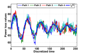
(a) $\delta=25$.

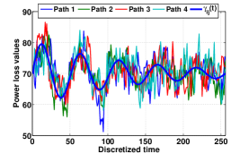
(b) $\delta=50$.

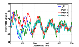
(c) $\delta=20$, $\beta=10$ for $\tau_{b}\leq 166$, $\beta=100$ for $166<\tau_{b}<333$ else $\beta=500$.

Figure 1: Wireless channel’s LTF stochastic behavior. Paths for the power loss (dB) modeled via SDE.

VII-A Congestion Control & Routing

In the sequel, we examine the case of applying only congestion control and routing, assuming the transmitter of each link $(i,j)$ has a constant power of $P_{ij}(t)=2W$, $\forall~{}t\in[0,T]$.

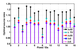
(a) Optimal source rates (bits/sec) vs. $\delta$.

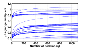
(b) Convergence of the Lagrange multipliers $\{\mu_{i}^{d}\}_{\forall i,d}$.

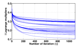
(c) Convergence of the Lagrange multipliers $\{l_{ij}\}_{\forall(i,j)}$.

Figure 2: Congestion control & routing: Optimal source rates and convergence of the Lagrange multipliers.

Fig. 2(a) shows the optimal source rates (i.e. after convergence since they change continuously with respect to the optimal Lagrange multipliers) for different choices of the diffusion coefficient $\delta$. It can be observed that as $\delta$ increases, random fluctuations to higher capacity values are exploited to offer increased optimal source rates, hence verifying numerically the statement of Theorem 3. It is important to note here that the noise level $\delta$ does not affect the mean power loss, as indicated in the proof of Theorem 3. In other words, if the mean power loss is used to determine capacity, higher capacity values due to random fluctuations cannot be tracked and exploited for increasing the source rates. Time-varying $\delta$ (TV) is also applied, and specifically $\delta=15sin(10\pi d/n)+35$ i.e. taking values between $\delta=20$ and $\delta=50$, thus leading to optimal source rates in between the ones corresponding to these two values of $\delta$. For benchmarking purposes, in Fig. 2(a) we have added the case of $\delta=0$, which corresponds to time-varying but deterministic channels. We observe that the optimal source rates achieved under deterministic wireless channels are the lowest (approximately the same as in the case of a low value of noise, i.e. the case that $\delta=5$), indicating the improvement in system’s performance when accounting for randomness.

Figs. 2(b), 2(c) depict the behavior of the proposed scheme considering convergence to the optimal Lagrange multipliers. We also study the impact of $T$ on the time to convergence and the achieved source rates. The value of $n$ is adapted for each $T$ as it is shown in Fig. 3(a). We observe that as the duration of the network’s operation, $T$, increases, the time to convergence also increases (Fig. 3(a)), while the achieved arrival source rates decrease for all flows (Fig. 3(b)). Finally, the behavior of the proposed algorithm in case of time varying $\beta_{ij}(t)$ with respect to the optimal source rates is shown in Fig. 3(c). We observe that when $\beta_{ij}(t)$ is high at the beginning (close to time $s=0$) the optimal rates are higher than when $\beta_{ij}(t)$ is initially low and increases later in time.

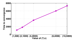
(a) Impact of $T$ on the time to convergence (iterations).

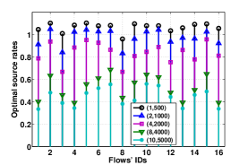
(b) Impact of $T$ on the optimal flows’ rates (bits/sec).

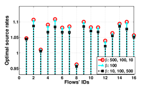
(c) Impact of time varying $\beta_{ij}(t)$ of the SDE (2) on the optimal flows’ rates (bits/sec).

Figure 3: Congestion control & routing: Study of the impact of $T$ and time-varying $\beta$ on convergence. In subfigure (c), black corresponds to $\beta=10$ for $\tau_{b}\leq 166$, $\beta=100$ for $166<\tau_{b}<333$ else $\beta=500$, red corresponds to $\beta=500$ for $\tau_{b}\leq 166$, $\beta=100$ for $166<\tau_{b}<333$ else $\beta=10$, and cyan corresponds to $\beta=100$.

VII-B Joint Scheduling, Routing, Congestion & Power Control Scheme

In order to evaluate the joint scheduling, routing, congestion and power control scheme, we assume that each link can vary its transmission power between $1W$ and $3W=P_{i,\max},~{}\forall i$. The network topology and traffic along with the rest of the parameters remain the same as in the previous experiments. Fig. 4(a) depicts the optimal transmission power at each repetition of channel state’s sampling derived from Eq. (VI) and the corresponding path of the link capacity. It is observed that the optimal power increases when power loss decreases (thus capacity increases) and attains low values for high values of power loss, as expected from the analysis of Section VI. Therefore, the transmission power increases only when there is an opportunity for an important capacity improvement due to random dips of power loss. On the contrary, transmission power is not wasted when the stochastic power loss does not support capacity increase. Fig. 4(b) shows the optimal source rates (i.e. after convergence) for different choices of the diffusion coefficient $\delta$. As in the previous case (Fig. 2(a)), it can be observed that as $\delta$ increases the optimal source rates increase for all flows. This is beyond the scope of Theorem 3, that does not account for power control and scheduling in the optimization problem. Fig. 4(b) also includes the optimal source rates when $\delta$ is time-varying (TV) and when channels are deterministic ($\delta=0$), leading to similar conclusions as in the case of congestion control and routing (Fig. 2(a)). Figs. 4(d), 4(e) depict the convergence to the optimal Lagrange multipliers.

Fig. 4(c) shows that the joint scheduling, routing, congestion and power control scheme improves the optimal source rates for all flows, compared to the congestion control and routing scheme. As also stated in [17], applying power control at the transmitter is like having channel state information at both the transmitter and the receiver which improves the network capacity compared with the case of constant power which is equivalent to having channel state information at the receiver’s side only. Furthermore, we study the expected per link transmission power over the entire time interval $[0,T]$ for the numerical experiments of Fig. 4. It can be easily computed that it is equal to $1.0399W$ for $\delta=50$, $1.2658W$ for $\delta=20$, $1.5634W$ for $\delta=5$, $1.6249W$ for $\delta=0$. On the one hand these values are much smaller than the constant power of $2W$ used to evaluate the routing and congestion control scheme (Fig. 2(a)), thus achieving a more “green” network operation in addition to throughput improvement (Figs. 4(b), 4(c)) leading to energy efficiency. On the other hand, we observe that as $\delta$ increases, the expected per link transmission power decreases, indicating the importance of taking randomness into account in operating wireless channels with energy efficiency.

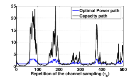
(a) Capacity (bits/sec) & optimal transmission power paths (W) ($\delta=20$).

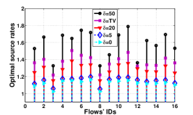
(b) Optimal source rates (bits/sec) vs. $\delta$.

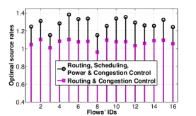
(c) Comparison of optimal source rates (bits/sec) with and without scheduling and power control ($\delta=20$).

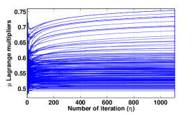
(d) Convergence of the Lagrange multipliers $\{\mu_{i}^{d}\}_{\forall i,d}$.

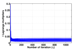
(e) Convergence of the Lagrange multipliers $\{l_{ij}\}_{\forall(i,j)}$.

Figure 4: Routing, Scheduling, Congestion & Power control.

VII-C Time Varying Utilities & Online Deployment

Finally, we study the case of time-varying utilities when applying routing and congestion control. The utilities take the form $U_{i}^{d}(\lambda_{i}^{d})=\frac{\log(\lambda_{i}^{d})}{t},~{}t\in[s,T],~{}s>0~{}\forall i,d:i\in S_{r}(d)$, i.e., they decrease with time modeling the decreasing willingness of users to produce high data amounts when approaching the end of the network’s operation. The optimal function to which the source rates converge over $[s,T]$ is depicted in Fig. 5(a). We observe that as time increases, it dominates over the Lagrange multiplier for the determination of the source rates (Eq. (23)).

At this point we will make another interesting observation regarding the online application of the proposed approach (Section VI) during the network’s operation which is initially discussed in Section V. In order to obtain an online algorithm for the network control, i.e. during the network operation, we may consider that the network decisions are taken at $\tau_{b}$ times when the channel is sampled, while also considering that $\tau_{b}\equiv\eta$. Then, we should consider the optimal control values in the interval $(\tau_{b},T]$ as “predicted” and the ones in the interval $[s,\tau_{b})$ as “corrections”. However, we should study under what conditions convergence is achieved (in practice) early enough (for small $\tau_{b}$) so that optimality with respect to the achieved value of $P_{2}$ is not affected. In Figs. 5(b), 5(c), it is shown that when increasing $n$, the time for convergence (according to the imposed criterion) of the proposed scheme is not significantly affected for time invariant utilities while it is affected in a concave manner for time varying utilities. As a result, if $n$ is large enough, the decisions taken at times $\tau_{b}$ will converge fast enough compared to the whole duration $T$. Therefore, the online application of the proposed approach during the network operation will be suboptimal only at the beginning barely affecting the optimal objective value of $P_{2}$.

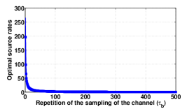
(a) Optimal functions (bits/sec) to which the source rates converge ($\delta=20$) for time varying utilities.

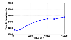
(b) Impact of $n$ on the time to convergence (iterations) for time varying utilities.

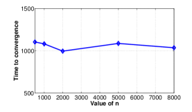
(c) Impact of $n$ on the time to convergence (iterations) for time invariant utilities.

Figure 5: Routing & Congestion control: Time varying utilities & Impact of $n$ on convergence.

VIII Conclusions

In this paper we presented, analyzed and evaluated a framework of NUM for performing routing, scheduling, congestion and power control under stochastic possibly non-stationary LTF or STF wireless channels modeled by SDEs. The continuous stochastic non-stationary wireless channels along with the consideration of transient phenomena lead to a problem formulation that can also tackle non-convex and time-varying objective functions in an optimal way. Power control aims at increasing users’ experience allowing for higher source rates while also improving the energy efficiency. In the case of LTF, we prove that higher values of the diffusion coefficient of the power loss lead to higher optimal users’ utilities, a fact that cannot be captured by the conventional NUM problem’s formulation. Numerical results evaluate the latter along with the convergence properties of our proposed algorithms and the effect of diverse parameters on it. The efficiency of power control and the conditions under which an online implementation of the proposed approach is possible are also investigated. Finally, our proposed NUM-based framework may constitute a core for devising efficient cross-layer algorithms for the network operation that incorporate transient or non-stationary phenomena.

IX Acknowledgment

This research is co-financed by the European Union (European Social Fund) and Hellenic national funds through the Operational Program ’Education and Lifelong Learning’ (NSRF 2007-2013). (under “ARISTEIA” 1260). M.L. acknowledges support from the NSRF Research Funding Program Thales: Optimal Management of Dynamical Systems of the Economy and the Environment MIS375586.

References

• [1] M. Chiang, “Balancing Transport and Physical Layers in Wireless Multihop Networks: Jointly Optimal Congestion Control and Power Control”, IEEE Journal on Selected Areas in Communications, Vol. 23, No. 1, pp. 104-116, Jan. 2005.
• [2] J. Papandriopoulos, S. Dey, J. S. Evans, “Optimal and Distributed Protocols for Cross-Layer Design of Physical and Transport Layers in MANETs”, IEEE/ACM Trans. on Networking, Vol. 16, No. 6, pp. 1392-1405, Dec. 2008.
• [3] C. Fischione, M. D’Angelo, M. Butussi, “Utility Maximization via Power and Rate Allocation with Outage Constraints in Nakagami-Lognormal Channels”, IEEE Trans. on Wireless Communications, Vol. 10, No. 4, pp. 1108-1120, April 2011.
• [4] D. O’Neill, B. Sim Thian, A. Goldsmith, S. Boyd, “Wireless NUM: Rate and Reliability Tradeoffs in Random Environment”, in Proc. of the IEEE Wireless Communications and Networking Conference (WCNC), pp. 1-6, April 2009.
• [5] S. Firouzabadi, D. O’Neill, A. Goldsmith, “Distributed Wireless Network Utility Maximization”, In Proc. of the 44th Annual Conference on Information Sciences and Systems (CISS), pp.1-6, March 2010.
• [6] A. G. Marques, N. Gatsis, G. B. Giannakis, “Optimal Cross-Layer Design of Wireless Fading Multi-hop Networks”, Cross Layer Designs in WLAN Systems, Leicester, UK:Troubador Publishing, 2011.
• [7] L. Chen, S. H. Low, M. Chiang, J. C. Doyle, “Cross-Layer Congestion Control, Routing and Scheduling Design in Ad Hoc Wireless Networks”, in Proc. of IEEE INFOCOM, pp. 1-13, April 2006.
• [8] L. Huang, S. Moeller, M. J. Neely, B. Krishnamachari, “LIFO-Backpressure Achieves Near-Optimal Utility-Delay Tradeoff”, IEEE/ACM Trans. on Networking, Vol. 21, No. 3, pp. 831-844, June 2013.
• [9] J. Chen, V. K. N. Lau, Y. Chen, “Distributive Network Utlity Maximization Over Time-Varying Fading Channels”, IEEE Transactions on Signal Processing, Vol. 59, No. 5, pp. 2395-2404, May 2011.
• [10] M. Olama, S. Djouadi, C. Charalambous, “Wireless Fading Channel Models: from Classical to Stochastic Differential Equations”, Stochastic Control, Chris Myers (Ed.), ISBN: 978-953-307-121-3, InTech, DOI: 10.5772/9738, Aug. 2010.
• [11] B. Oksendal, “Stochastic Differential Equations”, 6th Edition Springer-Verlag, 2003.
• [12] C. D. Charalambous, N. Menemenlis, “Stochastic Models for Short-term Multipath Fading Channels: Chi-square and Ornstein-Uhlenbeck Processes”, In Proc. of the 38th IEEE Conf. on Decision and Control, Vol. 5, pp. 4959-4964, 1999.
• [13] E. Stai, S. Papavassiliou, “User Optimal Throughput-Delay Trade-off in Multihop Networks under NUM Framework”, IEEE Communications Letters, Vol. 18, No. 11, pp. 1999-2002, Nov. 2014.
• [14] W. H. Fleming, H. M. Sooner, “Controlled Markov Processes and Viscosity Solutions”, 2nd Edition, Springer-Verlag, 2006.
• [15] E. Stai, M. Loulakis, S. Papavassiliou, “Congestion & Power Control of Wireless Multihop Networks over Stochastic LTF Channels”, in Proc. of IEEE Wireless Communications and Networking Conference (WCNC), pp. 1769-1774, March 2015.
• [16] G. Tychogiorgos, A. Gkelias, K. K. Leung, “A Non-Convex Distributed Optimization Framework and its Application to Wireless Ad-hoc Networks”, IEEE Trans. on Wireless Communications, Vol. 12, No. 9, pp. 4286-4296, September 2013.
• [17] A. Goldsmith, “Wireless Communications”, Cambridge University Press, 2005.
• [18] M. M. Olama, S. M. Djouadi, C. D. Charalambous, “Stochastic Differential Equations for Modeling, Estimation and Identification of Mobile-to-Mobile Communication Channels”, IEEE Transactions on Wireless Communications, Vol. 8, No. 4, pp. 1754-1763, April 2009.
• [19] C. D. Charalambous, R. J. C. Bultitude, X. Li, J. Zhan, “Modeling Wireless Fading Channels via Stochastic Differential Equations: Identification and Estimation Based on Noisy Measurements”, IEEE Transactions on Wireless Communications, Vol. 7, No. 2, pp. 434-439, February 2008.
• [20] M. J. Neely, “Delay-Based Network Utility Maximization”, in Proc. of IEEE INFOCOM, pp. 1-9, March 2010.
• [21] A. Eryilmaz, R. Srikant, “Joint Congestion Control, Routing and MAC for Stability and Fairness in Wireless Networks”, IEEE Journal on Selected Areas in Communications, Vol. 24, No. 8, pp. 1514-1524, August 2006.
• [22] A. Ribeiro, G. B. Giannakis, “Separation Principles in Wireless Networking”, IEEE Transactions on Information Theory, Vol. 56, No. 9, pp. 4488-4505, Sept. 2010.
• [23] D. P. Bertsekas, “Nonlinear Programming: 2nd Edition”, Athena Scientific, 2009.
• [24] N. Gatsis, A. Ribeiro, G. B. Giannakis, “A Class of Convergent Algorithms for Resource Allocation in Wireless Fading Networks”, IEEE Trans. on Wireless Communications, Vol. 9, No. 5, pp. 1808-1823, May 2010.
• [25] D. J. Higham, “An Algorithmic Introduction to Numerical Simulation of Stochastic Differential Equations”, SIAM REVIEW, Vol. 43, No. 3, pp. 525-546, 2001.
• [26] M. Olama, S. Djouadi, C. Charalambous, “Stochastic Power Control for Time-Varying Long-Term Fading Wireless Networks”, EURASIP Journal on Advances in Signal Processing, pp. 1-13, June 2006.
• [27] Y. Cui, E. M. Yeh, “Delay Optimal Control and its Connection to the Dynamic Backpressure Algorithm”, in Proc. of the IEEE International Symposium on Information Theory (ISIT), pp. 451-455, June-July 2014.
• [28] F. Hirsch, M. Yor, “Comparing Brownian Stochastic Integrals for the Convex Order”, Modern Stochastics and Apps., Springer Optimization and Its Apps., Springer Int’l Publishing, Vol. 90, pp. 3-19, 2014.
• [29] L. Georgiadis, M. J. Neely, L. Tassiulas, “Resource Allocation and Cross-Layer Control in Wireless Networks”, Foundations and Trends in Networking, Vol. 1, No. 1, pp. 1-144, 2006.