Quantum Feedback Amplification

Abstract

Quantum amplification is essential for various quantum technologies such as communication and weak-signal detection. However, its practical use is still limited due to inevitable device fragility that brings about distortion in the output signal or state. This paper presents a general theory that solves this critical issue. The key idea is simple and easy to implement: just a passive feedback of the amplifier’s auxiliary mode, which is usually thrown away. In fact, this scheme makes the controlled amplifier significantly robust, and furthermore it realizes the minimum-noise amplification even under realistic imperfections. Hence, the presented theory enables the quantum amplification to be implemented at a practical level. Also, a nondegenerate parametric amplifier subjected to a special detuning is proposed to show that, additionally, it has a broadband nature.

I Introduction

The amplifier is clearly one of the most important components incorporated in almost all current technological devices. The basic function of an autonomous amplifier is simply to transform an input signal $u$ to $y=Gu$ with gain $G>1$. However, such an amplifier is fragile in the sense that the device parameters change easily, and eventually distortion occurs in the output $y$. This was indeed a most serious issue which had prevented any practical use of amplifiers in, e.g., telecommunication. Fortunately, this issue was finally resolved back in 1927 by Black Black 77 ; Black 84 ; there are a huge number of textbooks and articles reviewing this revolutionary work, and here we refer to Refs. Mancini ; Bechhoefer . The key idea is the use of feedback shown in Fig. 1; that is, an autonomous amplifier called the “plant” is combined with a “controller” in such a way that a portion of the plant’s output is fed back to the plant through the controller. Then the output of the whole controlled system is given by

$$y=G^{(\rm fb)}u,~{}~{}~{}G^{({\rm fb})}=\frac{G}{1+GK},$$ (1)

where $K$ is the gain of the controller. Now, if the plant has a large gain $G\gg 1$, it immediately follows that $G^{({\rm fb})}\approx 1/K$. Hence, the whole system works as an amplifier, simply provided that the controller is a passive device (i.e., an attenuator) with $K<1$. Importantly, a passive device such as a resistor is very robust, and its parameters contained in $K$ almost do not change. This is the mechanism of robust amplification realized by feedback control. Note, of course, that this feedback architecture is the core of an operational amplifier (op-amp).

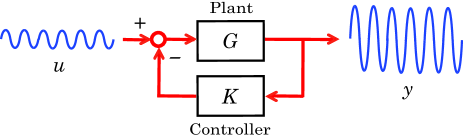
Figure 1: Classical feedback-amplification scheme: $G$ is the gain of an autonomous amplifier, and $K$ is the gain of a passive controller.

Surely there is no doubt about the importance of quantum amplifiers. A pertinent quantum counterpart to the classical amplifier is the phase-preserving linear amplifier Haus 62 ; Caves 82 (in what follows, we simply call it the “amplifier”). In fact, this system has a crucial role in diverse quantum technologies such as communication, weak-signal detection, and state processing Braunstein 01 ; Loudon 03 ; Leuchs 2008 ; Clerk 10 ; Hudelist 14 ; Ping Koy 14 ; Lehnert 14 ; Girvin 15 . In particular, recent substantial progress in both theory and experiments Josse 06 ; Devoret 10 ; Devoret 10b ; Nha 10 ; Furusawa 11 ; Caves 12 ; Clerk 14 ; Abdo 14 ; Clerk 15 ; Mabuchi 15 has further advanced this field. An important fact is that, however, an amplifier must be an active system powered by external energy sources, implying that its parameters are fragile and can change easily. Because of this parameter fluctuation, the amplified output signal or state suffers from distortion Slavik 2010 ; Caves 13 ; Dastjerdi 13 . As a consequence, the practical applicability of the quantum amplification is still severely limited. That is, we are now facing the same problem we had 90 years ago.

To make the discussion clear, let us here describe the general quantum-amplification process. Ideally the amplifier transforms a bosonic input mode $b_{1}$ to $\tilde{b}_{1}=g_{1}b_{1}+g_{2}b_{2}^{\dagger}$, where $b_{2}$ is an auxiliary mode, and the coefficients satisfy $|g_{1}|^{2}-|g_{2}|^{2}=1$ from $[\tilde{b}_{1},\tilde{b}_{1}^{\dagger}]=1$. Hence, the output $\tilde{b}_{1}$ is an amplified mode of $b_{1}$ with gain $|g_{1}|>1$. A typical example of an amplifier is the optical nondegenerate parametric amplifier (NDPA), in which case $g_{1}$ and $g_{2}$ are frequency dependent as shown later. However, note again that the system parameters, especially the coupling strength of the pumped crystal, cannot be kept exactly constant, and eventually the amplified output mode $\tilde{b}_{1}$ has to be distorted.

Now the motivation is clear; we need a quantum version of the feedback-amplification method described in the first paragraph. The contribution of this paper is, in fact, to develop a general theory for quantum feedback amplification that resolves the fragility issue of quantum amplifiers. The key idea is simple and easy to implement, i.e., feedback of the auxiliary output mode $\tilde{b}_{2}$ through a passive controller to the auxiliary input mode $b_{2}$. Indeed, it is proven that the whole controlled system possesses a strong robustness property against parameter fluctuations, which thus enables quantum amplifiers to be implemented at a practical level. This type of control scheme is, in general, called the coherent feedback Wiseman 94 ; James 08 ; Gough 09 ; Mabuchi 13 ; Kerckhoff 13 ; Yamamoto 14 , meaning that an output field is fed back to an input field through another quantum system without involving any measurement process; hence, an excess classical noise is not introduced in the feedback loop. Now note that the auxiliary output $\tilde{b}_{2}$ has some information about $\tilde{b}_{1}$ due to their entanglement, though $\tilde{b}_{2}$ is usually thrown away in the scenario of quantum amplification. Thus, we have an interpretation that the presented scheme utilizes the signal-recycling technique Yanbei 02 for reducing the sensitivity, unlike the conventional use of it for enhancing the sensitivity of the gravitational-wave detector.

In addition to the above-described main contribution, some important results are obtained. First, we see that the controlled system reaches the fundamental quantum noise limit Caves 82 even if some imperfections are present in the feedback loop. This means that precise fabrication of the feedback control is not necessary, which thus again emphasizes the feasibility of the presented scheme. Next, this paper proposes a type of NDPA subjected to a special detuning that circumvents the usual gain-bandwidth trade-off in the amplification process. A drawback of this modified amplifier is that, as will be shown, it is very sensitive to the parameter fluctuation. The presented theory has a distinct advantage in such a situation; that is, this issue can now be resolved by constructing a feedback loop. Therefore, as a concrete application of the theory, this paper proposes a robust, near-minimum-noise, and broadband amplifier.

Finally, note that there are a variety of quantum amplifiers considered in the literature such as an optical back-action evasion amplifier Yurke ; however, the schematic presented in this paper is essentially different from all those modifications in the following sense. While those modified amplifiers have their own purposes for improving the performance or achieving the goal in some specific subjects (e.g. back-action evasion), the feedback scheme is a device-independent and purpose-independent fundamental architecture that must be incorporated in all amplifiers. In fact, in the classical regime, the “operation” part of an op-amp has its own purpose (e.g., differentiation and integration), but any op-amp does not work without feedback.

II Model of phase-preserving linear quantum amplifier

Let us begin with a specific model: the NDPA. This is an optical cavity system with two internal modes $a_{1}$ and $a_{2}$. They are orthogonally polarized and obey the following Hamiltonian:

$$H=\omega_{1}a_{1}^{\dagger}a_{1}+\omega_{2}a_{2}^{\dagger}a_{2}+i\lambda(a_{1}^{\dagger}a_{2}^{\dagger}e^{-2i\omega_{0}t}-a_{1}a_{2}e^{2i\omega_{0}t}),$$

with $\lambda\in{\mathbb{R}}$ the coupling strength between the modes, $\omega_{i}$ the resonant frequencies of $a_{i}$, and $2\omega_{0}$ the pump frequency. Also, in the above expression the rotating-wave approximation is taken under the assumption $2\omega_{0}\approx\omega_{1}+\omega_{2}$. The system couples with a signal input $b_{1}$ and an auxiliary (idler) input $b_{2}$ with strength $\kappa$. Then, in the rotating frame at frequency $\omega_{0}$, the dynamics of the NDPA is given by the following Langevin equations Clerk 10 ; Ou ; Gardiner book :

$$\frac{da_{1}}{dt}=\Big{(}-\frac{\kappa}{2}-i\Delta_{1}\Big{)}a_{1}+\lambda a_{2}^{\dagger}-\sqrt{\kappa}b_{1},$$ (2)

$$\frac{da_{2}^{\dagger}}{dt}=\Big{(}-\frac{\kappa}{2}+i\Delta_{2}\Big{)}a_{2}^{\dagger}+\lambda a_{1}-\sqrt{\kappa}b_{2}^{\dagger},$$ (3)

where $\Delta_{1}=\omega_{1}-\omega_{0}$ and $\Delta_{2}=\omega_{2}-\omega_{0}$ are detuning. Also, the output equations (boundary conditions) are given by

$$\tilde{b}_{1}=\sqrt{\kappa}a_{1}+b_{1},~{}~{}~{}\tilde{b}_{2}^{\dagger}=\sqrt{\kappa}a_{2}^{\dagger}+b_{2}^{\dagger}.$$ (4)

Now the Laplace transformation of an observable $x_{t}$ in the Heisenberg picture is defined by

$$x(s):=\int_{0}^{\infty}e^{-st}x_{t}dt,$$

where ${\rm Re}(s)>0$. Then the Laplace transforms of $b_{1}$, etc., are connected by the following linear equations:

$$\tilde{b}_{1}(s)=g_{1}(s)b_{1}(s)+g_{2}(s)b_{2}^{\dagger}(s),$$

$$g_{1}(s)=\frac{(s-\frac{\kappa}{2}+i\Delta_{1})(s+\frac{\kappa}{2}-i\Delta_{2})-\lambda^{2}}{D(s)},~{}g_{2}(s)=\frac{-\kappa\lambda}{D(s)},$$

$$D(s)=\Big{(}s+\frac{\kappa}{2}+i\Delta_{1}\Big{)}\Big{(}s+\frac{\kappa}{2}-i\Delta_{2}\Big{)}-\lambda^{2}.$$

The stability analysis can be conducted in the Laplace domain; that is, for the amplifier to be stable, all roots of the characteristic equations of the transfer functions (i.e., poles) must lie in the left-hand complex plane. In the above case, particularly when $\Delta_{1}=\Delta_{2}=0$, the characteristic equation is $D(s)=s^{2}+\kappa s+\kappa^{2}/4-\lambda^{2}=0$; hence, $\kappa^{2}/4-\lambda^{2}>0$ must be satisfied to guarantee the stability of the NDPA.

The quantum-amplification process is described in the Fourier domain $s=i\omega$ with $\omega$ the frequency; that is, we consider the linear transformation at the steady state, $\tilde{b}_{1}(i\omega)=g_{1}(i\omega)b_{1}(i\omega)+g_{2}(i\omega)b_{2}^{\dagger}(i\omega)$. Note that $g_{1}$ and $g_{2}$ satisfy $|g_{1}(i\omega)|^{2}-|g_{2}(i\omega)|^{2}=1$ for all $\omega$. In particular, when $\Delta_{1}=\Delta_{2}=0$, the amplification gain at the resonant frequency $\omega=0$ is given by

$$|g_{1}(0)|=\frac{\kappa^{2}+4\lambda^{2}}{|\kappa^{2}-4\lambda^{2}|},$$

and it takes a large number nearly at the threshold $\lambda\approx\kappa/2-0$. Thus, $\tilde{b}_{1}$ is in fact an amplified mode of $b_{1}$ with gain $|g_{1}|$.

The above example can be generalized; any phase-preserving linear quantum amplifier is modeled as an open dynamical system with two inputs and two outputs. Let us represent the input-output relation in the Laplace domain as follows:

$$\left[\begin{array}[]{c}\tilde{b}_{1}(s)\\ \tilde{b}_{2}^{\dagger}(s)\\ \end{array}\right]=G(s)\left[\begin{array}[]{c}b_{1}(s)\\ b_{2}^{\dagger}(s)\\ \end{array}\right],$$ (9)

$$\hskip 16.99998ptG(s)=\left[\begin{array}[]{cc}G_{11}(s)&G_{12}(s)\\ G_{21}(s)&G_{22}(s)\\ \end{array}\right],$$ (12)

where $b_{1}(s)$ is the Laplace transformation of $b_{1}$, etc. The transfer function matrix $G(s)$ at $s=i\omega$ (i.e. the scattering matrix) satisfies

$$|G_{11}(i\omega)|^{2}-|G_{12}(i\omega)|^{2}=|G_{22}(i\omega)|^{2}-|G_{21}(i\omega)|^{2}=1,$$

$$G_{21}(i\omega)G_{11}^{*}(i\omega)-G_{22}(i\omega)G_{12}^{*}(i\omega)=0~{}~{}~{}\forall\omega.$$ (13)

Thus, $|G_{11}(i\omega)|$ represents the amplification gain.

III The quantum feedback amplification

III.1 Feedback configuration

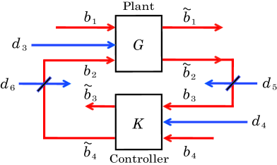
Figure 2: Coherent feedback configuration for the autonomous amplifier $G$ (plant). $d_{3},d_{4},d_{5}$, and $d_{6}$ are unwanted noisy input fields.

Our control scheme is based on coherent feedback; that is, the controller is also given by a quantum system and is connected to the plant through the input and output fields. Note that, if a measurement process is involved in the feedback loop, it inevitably introduces additional noise. Now we take a passive system (e.g. a beam splitter and an optical cavity) as the controller, with two inputs $b_{3},b_{4}$ and two outputs $\tilde{b}_{3},\tilde{b}_{4}$; note that a single-input and single-output passive system has a gain equal to 1 and thus does not work as an attenuator. We represent the input-output relation of this system in the Laplace domain as follows:

$$\left[\begin{array}[]{c}\tilde{b}_{3}^{\dagger}(s)\\ \tilde{b}_{4}^{\dagger}(s)\\ \end{array}\right]=K(s)\left[\begin{array}[]{c}b_{3}^{\dagger}(s)\\ b_{4}^{\dagger}(s)\\ \end{array}\right],$$ (18)

$$\hskip 16.99998ptK(s)=\left[\begin{array}[]{cc}K_{11}(s)&K_{12}(s)\\ K_{21}(s)&K_{22}(s)\\ \end{array}\right].$$ (21)

Here, the creation operator representation is taken to make the notation simple. Because of the passivity property, the transfer function matrix $K(s)$ is unitary in the Fourier domain; i.e., $K(i\omega)^{\dagger}K(i\omega)=I$ holds for all $\omega$.

We now consider connecting the controller to the plant. But unlike the classical case, where both the plant and the controller can be a single input-output system and arbitrary split or addition of signal is allowed, designing a feedback scheme in the quantum case is not trivial. For example, we could divide $\tilde{b}_{1}$ into two paths by a beam splitter and use one of them for feedback purpose, but in this case the resultant whole controlled system is not a minimum-noise amplifier. Instead, this paper proposes the following feedback connection as shown in Fig. 2:

$$\tilde{b}_{2}=b_{3},~{}~{}~{}b_{2}=\tilde{b}_{4},$$ (22)

which is, of course, equivalent to $\tilde{b}_{2}^{\dagger}=b_{3}^{\dagger}$ and $b_{2}^{\dagger}=\tilde{b}_{4}^{\dagger}$. Note that in Fig. 2 practical unwanted noises $d_{3},\ldots,d_{6}$ are illustrated, but these modes are ignored for the moment. From Eqs. (9), (18) and (22), the whole controlled system, with inputs $b_{1},b_{4}^{\dagger}$ and outputs $\tilde{b}_{1},\tilde{b}_{3}^{\dagger}$, has the following input-output relation in the Laplace domain:

$$\left[\begin{array}[]{c}\tilde{b}_{1}(s)\\ \tilde{b}_{3}^{\dagger}(s)\\ \end{array}\right]=\left[\begin{array}[]{cc}G_{11}^{({\rm fb})}(s)&G_{12}^{({\rm fb})}(s)\\ G_{21}^{({\rm fb})}(s)&G_{22}^{({\rm fb})}(s)\\ \end{array}\right]\left[\begin{array}[]{c}b_{1}(s)\\ b_{4}^{\dagger}(s)\\ \end{array}\right],$$

where

$$G_{11}^{({\rm fb})}=[G_{11}-K_{21}(G_{11}G_{22}-G_{12}G_{21})]/(1-K_{21}G_{22}),$$

$$G_{12}^{({\rm fb})}=(G_{12}K_{22})/(1-K_{21}G_{22}),$$

$$G_{21}^{({\rm fb})}=(G_{21}K_{11})/(1-K_{21}G_{22}),$$

$$G_{22}^{({\rm fb})}=[K_{12}+G_{22}(K_{11}K_{22}-K_{12}K_{21})]/(1-K_{21}G_{22}).$$

The matrix entries satisfy the condition corresponding to Eq. (II), i.e., $|G_{11}^{({\rm fb})}(i\omega)|^{2}-|G_{12}^{({\rm fb})}(i\omega)|^{2}=1$ $\forall\omega$, etc. Finally, as remarked in Sec. II, for the whole controlled system to be stable, the controller should be carefully designed so that all poles of $G_{ij}^{({\rm fb})}(s)$ must lie in the left-hand complex plane, as demonstrated in Sec. V.

III.2 Robust amplification via feedback

We now focus on the output of the controlled system in the Fourier domain, i.e.,

$$\tilde{b}_{1}(i\omega)=G_{11}^{({\rm fb})}(i\omega)b_{1}(i\omega)+G_{12}^{({\rm fb})}(i\omega)b_{4}^{\dagger}(i\omega),$$

and the amplification gain $|G_{11}^{({\rm fb})}(i\omega)|$ especially when the original gain $|G_{11}(i\omega)|$ is large. Note that $G_{11}^{({\rm fb})}$ looks somewhat different from the classical counterpart (1); hence, it is not immediate to see if $|G_{11}^{({\rm fb})}(i\omega)|$ can be approximated by a function of only the controller. Nonetheless, the analogous result to the classical case indeed holds as shown below.

For the proof we use Eq. (II) (below, we omit the variable $i\omega$). First, from $|G_{21}||G_{11}|=|G_{22}||G_{12}|$ together with the other two equations, we have $|G_{11}|=|G_{22}|$ and $|G_{12}|=|G_{21}|$. Also $G_{11}G_{22}-G_{12}G_{21}=G_{22}/G_{11}^{*}$ holds. Here, in the limit $|G_{11}|\rightarrow\infty$, it follows that

$$\frac{|G_{11}G_{22}-G_{12}G_{21}|}{|G_{11}|}=\frac{|G_{22}|}{|G_{11}|^{2}}=\frac{1}{|G_{11}|}\rightarrow 0.$$

This implies that $(G_{11}G_{22}-G_{12}G_{21})/|G_{11}|$ converges to zero in this limit. As a consequence, we have

$$|G_{11}^{({\rm fb})}|=\Big{|}\frac{G_{11}/|G_{11}|-K_{21}(G_{11}G_{22}-G_{12}G_{21})/|G_{11}|}{1/|G_{11}|-K_{21}G_{22}/|G_{11}|}\Big{|}$$

$$\hskip 20.00003pt\rightarrow\Big{|}\frac{G_{11}/|G_{11}|}{-K_{21}G_{22}/|G_{11}|}\Big{|}=\frac{1}{|K_{21}|}.$$

Hence, in the frequency range where the plant has a large gain $|G_{11}(i\omega)|\gg 1$, the whole controlled system amplifies the input $b_{1}(i\omega)$ with gain $|G_{11}^{({\rm fb})}(i\omega)|\approx 1/|K_{21}(i\omega)|>1$. Therefore we obtain the desirable quantum robust amplification method via feedback; that is, thanks to the fact that the passive controller is much more robust compared to the original amplifier, even if $G_{11}$ changes while maintaining a large value, the whole controlled system carries out robust amplification with stable gain $1/|K_{21}|$.

III.3 Feedback gain synthesis

Here we conduct a quantitative analysis on the robustness property, which provides a guideline for synthesizing the feedback gain $K$. To see the idea clearly, let us again consider the classical case (1). Let $\Delta G$ be the fluctuation that occurs in the plant $G$; then the fluctuation that occurs in the whole controlled system $G^{\rm(fb)}$ is calculated as

$$\Delta G^{\rm(fb)}=\frac{G+\Delta G}{1+(G+\Delta G)K}-\frac{G}{1+GK}\approx\frac{\Delta G}{(1+GK)^{2}},$$

which as a result leads to

$$\frac{\Delta G^{\rm(fb)}}{G^{\rm(fb)}}=\frac{1}{1+GK}\cdot\frac{\Delta G}{G}.$$ (23)

Hence, the gain sensitivity to the unwanted fluctuation can be reduced by the factor $1/|1+GK|$ by feedback. Equation (23) suggests to us not to design $G$ and $K$ separately; rather, what determines the performance of the controlled amplifier is the loop gain $GK$. Actually, while the controlled amplification gain, $G^{\rm(fb)}\approx 1/K$, can be made bigger by taking a smaller value of $K$, we should not design a too small $K$ such that $GK\approx 0$; in this case, Eq. (23) yields $\Delta G^{\rm(fb)}/G^{\rm(fb)}=\Delta G/G$, and thus there is no improvement in the sensitivity. The so-called Bode plot developed by Bode (e.g., see Ref. Bode book ) is a powerful graphical method for synthesizing $K$ as well as $G$, and it is now the standard tool for general feedback circuit design.

Now let us try to establish the quantum version of the above discussion. Note in advance that a straightforward calculation, like Eq. (23), cannot be carried out in the quantum case, but nonetheless a similar useful equation for determining the controller parameter $K_{21}$ is shown. First, due to $|G_{11}|=|G_{22}|$ and $G_{11}G_{22}-G_{12}G_{21}=G_{22}/G_{11}^{*}$, we find

$$G_{11}^{\rm(fb)}=\frac{|G_{11}|^{2}-K_{21}G_{22}}{G_{11}^{*}(1-K_{21}G_{22})}=\frac{G_{22}}{G_{11}^{*}}\cdot\frac{G_{22}^{*}-K_{21}}{1-K_{21}G_{22}},$$

which thus leads to

$$|G_{11}^{\rm(fb)}|=\frac{|G_{22}^{*}-K_{21}|}{|1-K_{21}G_{22}|}.$$

The fluctuation of the controlled gain is given by

$$\Delta|G_{11}^{\rm(fb)}|=\frac{|(G_{22}+\Delta G_{22})^{*}-K_{21}|}{|1-K_{21}(G_{22}+\Delta G_{22})|}-\frac{|G_{22}^{*}-K_{21}|}{|1-K_{21}G_{22}|}.$$

Then, from the general relation $|x+\epsilon|\approx|x|+(x\epsilon^{*}+x^{*}\epsilon)/2|x|$ with $x,\epsilon\in{\mathbb{C}}$ and $|\epsilon|\ll 1$, the normalized fluctuation of the amplification gain of the controlled system can be explicitly calculated as

$$\frac{\Delta|G_{11}^{\rm(fb)}|}{|G_{11}^{\rm(fb)}|}=\frac{1-|K_{21}|^{2}}{|G_{22}^{*}-K_{21}|^{2}}\cdot{\rm Re}\Big{(}\frac{G_{22}^{*}-K_{21}}{1-K_{21}G_{22}}\Delta G_{22}\Big{)}.$$ (24)

Next, noting that $|G_{22}|=|G_{11}|\gg 1$ and thus $|K_{21}|\ll|G_{22}|$, we find from Eq. (24) that

$$\Big{|}\frac{\Delta|G_{11}^{\rm(fb)}|}{|G_{11}^{\rm(fb)}|}\Big{|}\approx\frac{1}{|G_{22}|^{2}}\cdot\Big{|}{\rm Re}\Big{(}\frac{G_{22}^{*}}{1-K_{21}G_{22}}\Delta G_{22}\Big{)}\Big{|}.$$

Thus, from the general relation $|{\rm Re}(xy)|\leq|x||y|$ with $x,y\in{\mathbb{C}}$, it follows that

$$\Big{|}\frac{\Delta|G_{11}^{\rm(fb)}|}{|G_{11}^{\rm(fb)}|}\Big{|}\leq\frac{1}{|1-K_{21}G_{22}|}\cdot\frac{|\Delta G_{22}|}{|G_{22}|}.$$ (25)

Equation (25) has a similar form to Eq. (23) and indeed provides us a guideline for feedback design. That is, as in the classical case, the balance of $K_{21}$ and $G_{22}$ determines the ability of the controlled system to suppress the fluctuation (note that $|\Delta G_{22}|\geq\Delta|G_{22}|=\Delta|G_{11}|$). In particular, we now deduce a similar conclusion as in the classical case; if we choose a too small $K_{21}$ in addition to $|G_{11}|\gg 1$ such that the loop gain $K_{21}G_{22}$ is almost zero, then substituting the relation

$$\Delta|G_{11}|=\Delta|G_{22}|={\rm Re}(G_{22}^{*}\Delta G_{22})/|G_{22}|$$

into Eq. (24) we obtain $\Delta|G_{11}^{\rm(fb)}|/|G_{11}^{\rm(fb)}|=\Delta|G_{11}|/|G_{11}|$. That is, in this case the fluctuation is not at all suppressed via feedback. To design an appropriate controller gain $K_{21}$, the Bode plot of the loop gain $K_{21}(i\omega)G_{22}(i\omega)$ is useful.

IV Quantum noise limit

Let us define the noise magnitude of $b$ by

$$\langle{|\Delta b|^{2}}\rangle:=\frac{1}{2}\langle{\Delta b\Delta b^{\dagger}+\Delta b^{\dagger}\Delta b}\rangle,~{}~{}~{}\Delta b=b-\langle{b}\rangle.$$

Then, through the ideal amplification process $\tilde{b}_{1}=g_{1}b_{1}+g_{2}b_{2}^{\dagger}$, the noise magnitude must be also amplified as $\langle{|\Delta\tilde{b}_{1}|^{2}}\rangle=|g_{1}|^{2}\langle{|\Delta b_{1}|^{2}}\rangle+|g_{2}|^{2}/2$, where $b_{2}$ is assumed to be in the vacuum. This implies the degradation of the signal-to-noise ratio:

$$\widetilde{{\rm(S/N)}}=\frac{|\langle{\tilde{b}_{1}}\rangle|^{2}}{\langle{|\Delta\tilde{b}_{1}|^{2}}\rangle}=\frac{|\langle{b_{1}}\rangle|^{2}}{\langle{|\Delta b_{1}|^{2}}\rangle+{\cal A}}<\frac{|\langle{b_{1}}\rangle|^{2}}{\langle{|\Delta b_{1}|^{2}}\rangle}={\rm(S/N)}.$$

Hence, the added noise

$${\cal A}:=\frac{|g_{2}|^{2}}{2|g_{1}|^{2}}=\frac{|g_{1}|^{2}-1}{2|g_{1}|^{2}}$$

quantifies the fidelity of the amplification process Haus 62 ; Caves 82 . In particular, in the large amplification limit $|g_{1}|\rightarrow\infty$ we find ${\cal A}\rightarrow 1/2$, which is called the quantum noise limit.

Up to now, the ideal setup is assumed, and the controlled system is driven by only the signal $b_{1}$ and the auxiliary input $b_{4}$, implying that it actually reaches the quantum noise limit in the large amplification limit. Hence, here we consider the following general case where some excess noise exists, as illustrated in Fig. 2; the plant is subjected to an unwanted noise $d_{3}$ that enters into the system in the form $\tilde{b}_{1}=G_{11}b_{1}+G_{12}b_{2}^{\dagger}+G_{13}d_{3}$; the controller is also affected by a noise $d_{4}$; furthermore, the feedback transmission lines are lossy, which is modeled by inserting fictitious beam splitters with additional inputs $d_{5}$ and $d_{6}$. Note that $d_{3},\ldots,d_{6}$ are all annihilation modes. Then the output of the whole controlled system has the form

$$\tilde{b}_{1}=G_{11}^{\rm(fb)}b_{1}+G_{12}^{\rm(fb)}b_{2}^{\dagger}+G_{13}^{\rm(fb)}d_{3}+G_{14}^{\rm(fb)}d_{4}^{\dagger}+G_{15}^{\rm(fb)}d_{5}^{\dagger}+G_{16}^{\rm(fb)}d_{6}^{\dagger}.$$

Then, if the excess noises are all vacuum, the added noise in the feedback-controlled amplification process, denoted by ${\cal A}^{\rm(fb)}$, satisfies

$$\lim_{|G_{11}^{\rm(fb)}|\rightarrow\infty}{\cal A}^{\rm(fb)}=\lim_{|G_{11}|\rightarrow\infty}{\cal A}^{\rm(o)}=\frac{1}{2}+\frac{|G_{13}|^{2}}{|G_{11}|^{2}},$$ (26)

where ${\cal A}^{\rm(o)}$ is the added noise of the plant. The proof of Eq. (26), including the detailed forms of $G_{k}^{\rm(fb)}$, is given in Appendix A. This is a very useful result for the following reasons. First, in the large amplification limit the two added noises ${\cal A}^{\rm(fb)}$ and ${\cal A}^{\rm(o)}$ are equal; as a consequence the second term in the right-hand side of Eq. (26) is a function of only the plant and cannot be further altered by feedback control. Hence, we have the following no-go theorem: If the original amplifier does not reach the quantum noise limit (i.e., $\lim_{|G_{11}|\rightarrow\infty}|G_{13}|/|G_{11}|>0$), the controller can never remove this excess noise. On the other hand, notably, the imperfections contained in the controller and the feedback transmission lines do not appear in Eq. (26). This means that a very accurate fabrication of the feedback controller is not necessarily required, which is a desirable fact from a practical viewpoint. Thus, if the original amplifier operates with the minimum added noise, the controlled system reaches the quantum noise limit as well even if some imperfections are present in the feedback loop.

V Application to optical broadband amplification

In any practical situation, it is important to carefully engineer an amplifier so that it has a proper frequency bandwidth in which nearly constant amplification gain is realized. On the other hand, it is known in both the classical and quantum cases that, particularly for an amplifier with a single pole, the effective bandwidth becomes smaller if the amplification gain is taken to be bigger. That is, there is a gain-bandwidth constraint. However, this constraint is not necessarily applied to a more complex amplifier with multiple poles. In fact, recently in Ref. Clerk 14 , the authors propose a hybrid amplifier composed of two cavity modes and an additional opto-mechanical mode that circumvents the gain-bandwidth constraint. In this section, we study another system that is also free from this constraint, that yet does not need an additional degree of freedom. Then, the effectiveness of feedback is discussed, demonstrating its ability to make the system robust.

V.1 NDPA with special detuning

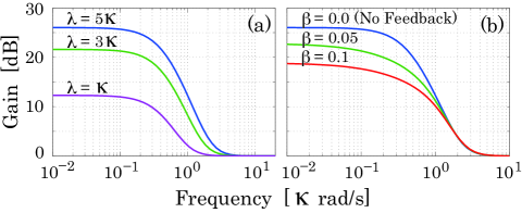
Figure 3: (a) Gain profile of the specially detuned NDPA without feedback. (b) Gain profile of the feedback-controlled system with parameters $\lambda=5\kappa$ and various $\beta$.

The plant system is the NDPA with dynamics (2), (3) and output (4). Here we consider the ideal case where the unwanted noises $d_{3},\ldots,d_{6}$ shown in Fig. 2 are not present. Without any invention, this system is subject to a gain-bandwidth constraint Clerk 10 , but now let us take the specific detuning as $\Delta_{1}=\Delta_{2}=\lambda$. The transfer function matrix of this system is then given by

$$G(s)=\frac{1}{(s+\kappa/2)^{2}}\left[\begin{array}[]{cc}s^{2}-\kappa^{2}/4+i\kappa\lambda&-\kappa\lambda\\ -\kappa\lambda&s^{2}-\kappa^{2}/4-i\kappa\lambda\\ \end{array}\right].$$

The maximum gain is $|G_{11}(0)|=\sqrt{1+16\lambda^{2}/\kappa^{2}}$, which becomes larger by increasing $\lambda$. Remarkably, this amplification can be carried out without sacrificing the bandwidth. Figure 3 (a) shows the three cases corresponding to $\lambda=\kappa,3\kappa,5\kappa$, all of which have the same effective bandwidth $\sim\kappa/10$. A clear advantage of this system is in its implementability; that is, it is composed of only optical devices, and there is no need to prepare an auxiliary system such as an opto-mechanical oscillator. Also, note that the system is always stable (the pole of the transfer function matrix is $-\kappa/2$); that is, in a proper parameter regime such that the linearized model given by Eqs. (2) and (3) is valid , there is no clear upper bound on $\lambda$, in contrast to the standard NDPA which imposes $|\lambda|<\kappa/2$.

V.2 The feedback effect

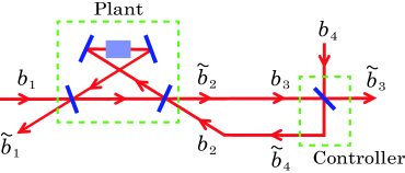
Figure 4: The NDPA (plant) and its coherent feedback; by simply feeding the auxiliary output $\tilde{b}_{2}$ back to the auxiliary input $b_{2}$ through just a beam splitter, the robustness property is drastically improved, as discussed in the main text.

Next, let us consider the feedback control of this amplifier, again in the ideal setup. Here, as shown in Fig. 4, a beam splitter with transmissivity $\alpha$ and reflectivity $\beta$ is taken as a controller. This device has no internal dynamics, and its transfer function matrix is constant:

$$K(s)=\left[\begin{array}[]{cc}\alpha&\beta\\ \beta&-\alpha\\ \end{array}\right],~{}~{}~{}\alpha,\beta\in{\mathbb{R}}.$$

Thus, $K_{21}=\beta$ represents the attenuation level. The amplification gain of the whole controlled system is then

$$G_{11}^{({\rm fb})}(s)=\frac{(1-\beta)s^{2}+\beta\kappa s-(1+\beta)\kappa^{2}/4+i\kappa\lambda}{(1-\beta)s^{2}+\kappa s+(1+\beta)\kappa^{2}/4+i\beta\kappa\lambda}.$$

This expression shows that, as expected from the general theory discussed in Sec. III B, in the limit $|G_{11}(i\omega)|\rightarrow\infty$ (i.e., $\lambda\rightarrow\infty$) the gain becomes $|G_{11}^{({\rm fb})}(i\omega)|\rightarrow 1/\beta$ in a certain frequency bandwidth. To determine the attenuation level $\beta$, we need the stability condition; it is shown in Appendix B that, for all the poles of $G_{11}^{({\rm fb})}(s)$ to lie in the left-hand complex plane, the parameters must satisfy

$$|\lambda|<\frac{\kappa}{2}\sqrt{\frac{1+\beta}{\beta^{2}(1-\beta)}}.$$ (27)

This yields $|\beta|<\kappa/2|\lambda|$ when $\beta^{2}\ll 1$; hence, let us here choose $\lambda=5\kappa$, leading to $|\beta|<0.1$. Figure 3 (b) shows the gain $|G_{11}^{({\rm fb})}(i\omega)|$ for the two cases $\beta=0.1$ and $\beta=0.05$ together with the plot without feedback (i.e., $\beta=0$). We then observe that the gain of the controlled amplifier becomes smaller than that without feedback; in exchange for this reduced gain, the controlled amplifier obtains a great robustness property against the parameter fluctuation as demonstrated later. Note that a larger value of $\beta$ (thus smaller amplification gain) induces a wider frequency bandwidth; hence, the controlled NDPA has the gain-bandwidth constraint. But the point here is rather that the gain and bandwidth can be easily tuned by just changing the reflectivity of the beam splitter. That is, an easily adjustable amplification can be realized, and this is also a clear advantage of feedback.

V.3 Robustness property

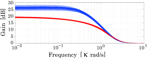
Figure 5: The upper blue lines represent the gain profile of the specially detuned NDPA without feedback, $|G_{11}(i\omega)|$, while the lower red lines correspond to the controlled case $|G_{11}^{\rm(fb)}(i\omega)|$ with $\beta=0.1$. In both cases, $\lambda_{0}=5\kappa$.

As repeatedly emphasized in this paper, the main strength of feedback is that the controlled system possesses a robustness property. To see this, let us consider an imperfect case as follows. First, the device parameters are fragile; the coupling strength $\lambda$ fluctuates in such a way that $\lambda=(1+0.1\epsilon_{0})\lambda_{0}$, where $\lambda_{0}$ is the nominal value; similarly, the detunings $\Delta_{1}$ and $\Delta_{2}$ can be slightly deviated from $\lambda$, which is modeled by $\Delta_{1}=(1+0.001\epsilon_{1})\lambda$ and $\Delta_{2}=(1+0.001\epsilon_{2})\lambda$. Here $(\epsilon_{0},\epsilon_{1},\epsilon_{2})$ are independent random variables subjected to the uniform distribution in $[-1,1]$. In addition to this fragility, we assume that the signal mode $a_{1}$ is subjected to optical loss, which is modeled by adding the extra term $-\gamma a_{1}/2-\sqrt{\gamma}d_{3}$ to the right-hand side of Eq. (2), with $\gamma$ the magnitude of the loss and $d_{3}$ the unwanted vacuum noise. The feedback transmission lines are also lossy, which is modeled by Eq. (33).

The blue lines in Fig. 5 are 50 sample values of the autonomous gain $|G_{11}(i\omega)|$ in the case $\lambda_{0}=5\kappa$ and $\alpha_{1}=\alpha_{2}=0.99$. That is, in fact, due to the parameter fluctuation described above, the amplifier becomes fragile and the amplification gain significantly varies. Nonetheless, this fluctuation can be suppressed by feedback; the red lines in Fig. 5 are 50 sample values of the controlled gain $|G_{11}^{\rm(fb)}(i\omega)|$ with attenuation level $\beta=0.1$, whose fluctuation is indeed much smaller than that of $|G_{11}(i\omega)|$ . (Note that, because the fluctuation of $|G_{11}^{\rm(fb)}(i\omega)|$ is very small, the set of sample values looks like a thick line.) That is, the controlled system is certainly robust against the realistic fluctuation of the device parameters.

V.4 Added noise

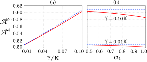
Figure 6: The added noise of the controlled amplifier with attenuation level $\beta=0.1$ and that of the non-controlled one (i.e., $\beta=0$) versus (a) $\gamma/\kappa$ with fixed $\alpha_{1}=\alpha_{2}=0.5$, and (b) $\alpha_{1}=\alpha_{2}$ with fixed $\gamma/\kappa$. In both figures, the red solid lines represent ${\cal A}^{\rm(fb)}$, while the blue dotted lines are ${\cal A}^{\rm(o)}$, at $\omega=0$.

Finally, let us investigate how much the excess noise is added to the output of the controlled or noncontrolled specially detuned NDPA. Again we set $\lambda_{0}=5\kappa$, and the feedback control is conducted with attenuation level $\beta=0.1$. Also, the same imperfections considered in the previous subsection are assumed; that is, the system suffers from the signal loss (represented with $\gamma$) and the probabilistic fluctuation of the parameters ($\lambda,\Delta_{1},\Delta_{2}$); furthermore, the feedback control is implemented with the lossy transmission lines (represented with $\alpha_{1}$ and $\alpha_{2}$).

With this setup Fig. 6 is obtained, where the red solid lines are sample values of the added noise at the center frequency $\omega=0$ for the controlled system, ${\cal A}^{\rm(fb)}$ given by Eq. (A), while the blue dotted lines represent those of the non-controlled system, ${\cal A}^{\rm(o)}$ given by Eq. (A). (In the figure it appears that six thick lines are plotted, but each is the set of 50 sample values.) Figure 6 (a) shows ${\cal A}^{\rm(fb)}$ and ${\cal A}^{\rm(o)}$ versus the signal loss rate $\gamma/\kappa$, where for the controlled system we fix $\alpha_{1}=\alpha_{2}=0.5$ (that is, the feedback transmission lines are very lossy). Also, Fig. 6 (b) shows the added noise as a function of $\alpha_{1}=\alpha_{2}$, with fixed signal loss $\gamma/\kappa$.

The first crucial point is that, in both figures (a) and (b), ${\cal A}^{\rm(fb)}$ and ${\cal A}^{\rm(o)}$ are close to each other. This is the fact that can be expected from Eq. (26), which states that ${\cal A}^{\rm(fb)}$ and ${\cal A}^{\rm(o)}$ coincide in the large amplification limit. It is also notable that, for all sample values, ${\cal A}^{\rm(fb)}$ is smaller than ${\cal A}^{\rm(o)}$ ; in other words, the feedback controller reduces the added noise, although in the large amplification limit this effect becomes negligible as proven in Eq. (26). Another important feature is that, as seen in Fig. 6 (a), the signal loss $\gamma$ is the dominant factor increasing the added noise, and the feedback loss $1-\alpha_{1}(=1-\alpha_{2})$ does not have a large impact on it, as seen in Fig. 6 (b). As consequence, when $\gamma$ is small, the controlled amplifier can perform amplification nearly at the quantum noise limit $1/2$, with almost no dependence on the feedback loss; this fact is also consistent with Eq. (26).

In summary, the specially detuned NDPA with feedback control functions as a robust, near-minimum-noise (if $\gamma\ll\kappa$), and broadband amplifier.

VI Conclusion

The presented feedback control theory resolves the critical fragility issue in phase-preserving linear quantum amplifiers. The theory is general and thus applicable to many different physical setups, such as optics, opto-mechanics, superconducting circuits, and their hybridization. Moreover, the feedback scheme is simple and easy to implement, as demonstrated in Sec. V. Note also that the case of phase-conjugating amplification Cerf 01 ; Leuchs 2007 can be discussed in a similar way; see Appendix C.

In a practical setting, the controller synthesis problem becomes complicated, implying the need to develop a more sophisticated quantum feedback amplification theory, which indeed was established in the classical case Mancini ; Bode book ; Astrom Murray . The combination of those classical approaches with the quantum control theory Doherty 2000 ; WisemanBook ; KurtBook should advance this research direction. Another interesting future work is to study genuine quantum-mechanical settings, e.g., probabilistic amplification Caves 13 ; Ralph 09 ; Pryde 10 ; Ralph 14 . Finally, note that feedback control is used in order to reach the quantum noise limit, in a different amplification scheme (the so-called op-amp mode) Clerk 10 ; Courty 99 ; connection to these works is also to be investigated.

This work was supported in part by JSPS Grant-in-Aid No. 15K06151.

Appendix A Proof of Eq. (12)

First, we again describe the setup of the imperfect system depicted in Fig. 2, in a more detailed way. The plant system is subjected to an unwanted noise $d_{3}$, such that the input-output relationship is given by

$$\left[\begin{array}[]{c}\tilde{b}_{1}(s)\\ \tilde{b}_{2}^{\dagger}(s)\\ \end{array}\right]=\left[\begin{array}[]{ccc}G_{11}(s)&G_{12}(s)&G_{13}(s)\\ G_{21}(s)&G_{22}(s)&G_{23}(s)\\ \end{array}\right]\left[\begin{array}[]{c}b_{1}(s)\\ b_{2}^{\dagger}(s)\\ d_{3}(s)\\ \end{array}\right].$$ (28)

The transfer function matrix in this case satisfies

$$|G_{11}|^{2}-|G_{12}|^{2}+|G_{13}|^{2}=|G_{22}|^{2}-|G_{21}|^{2}-|G_{23}|^{2}=1,$$

$$G_{21}G_{11}^{*}-G_{22}G_{12}^{*}+G_{23}G_{13}^{*}=0,$$ (29)

for all $s=i\omega$. Thus, the added noise of the plant system is given by

$${\cal A}^{\rm(o)}=\frac{|G_{12}|^{2}+|G_{13}|^{2}}{2|G_{11}|^{2}}=\frac{|G_{11}|^{2}+2|G_{13}|^{2}-1}{2|G_{11}|^{2}}$$

$$\hskip 11.99998pt=\frac{1}{2}-\frac{1}{2|G_{11}|^{2}}+\frac{|G_{13}|^{2}}{|G_{11}|^{2}}.$$ (30)

This leads to

$$\lim_{|G_{11}|\rightarrow\infty}{\cal A}^{\rm(o)}=\frac{1}{2}+\frac{|G_{13}|^{2}}{|G_{11}|^{2}},$$ (31)

where the second term is assumed to exist. Note that in a more general setup some creation noise modes (e.g. $d_{3}^{\dagger}$) can be contained in Eq. (28), but this modification does not change the conclusion. The controller also contains an unwanted noise field $d_{4}$ in the following form:

$$\left[\begin{array}[]{c}\tilde{b}_{3}^{\dagger}(s)\\ \tilde{b}_{4}^{\dagger}(s)\\ \end{array}\right]=\left[\begin{array}[]{ccc}K_{11}(s)&K_{12}(s)&K_{13}(s)\\ K_{21}(s)&K_{22}(s)&K_{23}(s)\\ \end{array}\right]\left[\begin{array}[]{c}b_{3}^{\dagger}(s)\\ b_{4}^{\dagger}(s)\\ d_{4}^{\dagger}(s)\\ \end{array}\right].$$ (32)

The point here is that only the creation modes appear in Eq. (32), unlike Eq. (28) that involves both creation and annihilation modes; this is indeed due to the passivity property of the controller. Finally, the transmission lines (optical fields) for feedback are assumed to be lossy. This setting is modeled by inserting two fictitious beam splitters; the beam splitter in the output field $\tilde{b}_{2}$ has transmissivity $\alpha_{1}$ and reflectivity $\delta_{1}$, and also the beam splitter in the output field $\tilde{b}_{4}$ has transmissivity $\alpha_{2}$ and reflectivity $\delta_{2}$ (we assume $\alpha_{i},\delta_{i}\in{\mathbb{R}}$ without loss of generality). Then, the coherent feedback connection is represented by the following relations:

$$b_{3}^{\dagger}=\alpha_{1}\tilde{b}_{2}^{\dagger}+\delta_{1}d_{5}^{\dagger},~{}~{}~{}b_{2}^{\dagger}=\alpha_{2}\tilde{b}_{4}^{\dagger}+\delta_{2}d_{6}^{\dagger}.$$ (33)

Combining Eqs. (28), (32), and (33), we end up with

$$\tilde{b}_{1}=G_{11}^{\rm(fb)}b_{1}+G_{12}^{\rm(fb)}b_{4}^{\dagger}+G_{13}^{\rm(fb)}d_{3}+G_{14}^{\rm(fb)}d_{4}^{\dagger}+G_{15}^{\rm(fb)}d_{5}^{\dagger}+G_{16}^{\rm(fb)}d_{6}^{\dagger},$$

where

$$G_{11}^{\rm(fb)}=[G_{11}-\alpha_{1}\alpha_{2}K_{21}(G_{11}G_{22}-G_{12}G_{21})]/{\bf G},$$

$$G_{13}^{\rm(fb)}=[G_{13}-\alpha_{1}\alpha_{2}K_{21}(G_{13}G_{22}-G_{12}G_{23})]/{\bf G},$$

$$G_{12}^{\rm(fb)}=\alpha_{2}G_{12}K_{22}/{\bf G},~{}~{}~{}G_{14}^{\rm(fb)}=\alpha_{2}G_{12}K_{23}/{\bf G},$$

$$G_{15}^{\rm(fb)}=\alpha_{2}\delta_{1}G_{12}K_{21}/{\bf G},~{}~{}~{}G_{16}^{\rm(fb)}=\delta_{2}G_{12}/{\bf G},$$

and ${\bf G}=1-\alpha_{1}\alpha_{2}K_{21}G_{22}$. Note that the transfer functions satisfy at $s=i\omega$

$$|G_{11}^{\rm(fb)}|^{2}-|G_{12}^{\rm(fb)}|^{2}+|G_{13}^{\rm(fb)}|^{2}$$

$$\hskip 20.00003pt\mbox{}-|G_{14}^{\rm(fb)}|^{2}-|G_{15}^{\rm(fb)}|^{2}-|G_{16}^{\rm(fb)}|^{2}=1.$$ (34)

Here we derive some preliminary results that are used later. First, Eq. (29) leads to $|G_{21}G_{11}^{*}-G_{22}G_{12}^{*}|^{2}=|G_{23}|^{2}|G_{13}|^{2}$; together with the other two equations, we then have

$$\Big{|}\frac{G_{11}G_{22}-G_{12}G_{21}}{G_{11}}\Big{|}^{2}$$

$$\hskip 20.00003pt=1+\Big{|}\frac{G_{22}}{G_{11}}\Big{|}^{2}-\frac{|G_{12}|^{2}+|G_{21}|^{2}+1}{|G_{11}|^{2}}.$$ (35)

Similarly,

$$\Big{|}\frac{G_{13}G_{22}-G_{12}G_{23}}{G_{11}}\Big{|}^{2}=\Big{|}\frac{G_{22}}{G_{11}}\Big{|}^{2}-\Big{|}\frac{G_{23}}{G_{11}}\Big{|}^{2}-1.$$ (36)

Furthermore, we can prove that $|G_{22}/G_{11}|\rightarrow 0$ never hold in the limit of $|G_{11}|\rightarrow\infty$ as follows. If $|G_{22}/G_{11}|\rightarrow 0$, this leads to $G_{21}/G_{11}\rightarrow 0$ and $G_{23}/G_{11}\rightarrow 0$, and furthermore, $|G_{12}/G_{11}|\rightarrow 1$ and $|G_{13}|\rightarrow 1$ from Eqs. (29) and (A); then using Eq. (36) we have $G_{23}\rightarrow 0$ and accordingly $G_{21}G_{11}^{*}-G_{22}G_{12}^{*}\rightarrow 0$, which leads to a contradiction.

Now we are concerned with the amplification gain $|G_{11}^{{\rm(fb)}}|$ in the limit $|G_{11}|\rightarrow\infty$. It is given by

$$|G_{11}^{\rm(fb)}|=\Big{|}\frac{1-\alpha_{1}\alpha_{2}K_{21}(G_{11}G_{22}-G_{12}G_{21})/G_{11}}{1/G_{11}-\alpha_{1}\alpha_{2}K_{21}(G_{22}/G_{11})}\Big{|}$$

$$\hskip 2.5pt\approx\Big{|}\frac{-1}{\alpha_{1}\alpha_{2}K_{21}(G_{22}/G_{11})}+\frac{(G_{11}G_{22}-G_{12}G_{21})/G_{11}}{G_{22}/G_{11}}\Big{|}.$$

The second term is upper bounded, because from Eq. (A)

$$\Big{|}\frac{G_{11}G_{22}-G_{12}G_{21}}{G_{11}}\Big{|}\Big{/}\Big{|}\frac{G_{22}}{G_{11}}\Big{|}\leq\sqrt{1+1\Big{/}\Big{|}\frac{G_{22}}{G_{11}}\Big{|}^{2}}$$ (37)

and also $|G_{22}/G_{11}|$ does not converge to zero. Therefore, we need $K_{21}(G_{22}/G_{11})\rightarrow 0$ (hence, $K_{21}\rightarrow 0$) to have the condition $|G_{11}^{{\rm(fb)}}|\rightarrow\infty$.

Finally, the added noise in the controlled system is computed as follows:

$${\cal A}^{\rm(fb)}=\frac{|G_{12}^{\rm(fb)}|^{2}+|G_{13}^{\rm(fb)}|^{2}+|G_{14}^{\rm(fb)}|^{2}+|G_{15}^{\rm(fb)}|^{2}+|G_{16}^{\rm(fb)}|^{2}}{2|G_{11}^{\rm(fb)}|^{2}}$$

$$\hskip 15.00002pt=\frac{|G_{11}^{\rm(fb)}|^{2}+2|G_{13}^{\rm(fb)}|^{2}-1}{2|G_{11}^{\rm(fb)}|^{2}}$$

$$\hskip 15.00002pt=\frac{1}{2}-\frac{1}{2|G_{11}^{\rm(fb)}|^{2}}+\frac{|G_{13}^{\rm(fb)}|^{2}}{|G_{11}^{\rm(fb)}|^{2}},$$ (38)

where Eq. (A) is used; also note that all the noise fields are now vacuum. The third term is given by

$$\frac{|G_{13}^{\rm(fb)}|^{2}}{|G_{11}^{\rm(fb)}|^{2}}=\Big{|}\frac{G_{13}-\alpha_{1}\alpha_{2}K_{21}(G_{13}G_{22}-G_{12}G_{23})}{G_{11}-\alpha_{1}\alpha_{2}K_{21}(G_{11}G_{22}-G_{12}G_{21})}\Big{|}^{2}.$$ (39)

Then from Eq. (A) we find

$$\Big{|}K_{21}\cdot\frac{G_{11}G_{22}-G_{12}G_{21}}{G_{11}}\Big{|}^{2}\leq|K_{21}|^{2}+\Big{|}K_{21}\cdot\frac{G_{22}}{G_{11}}\Big{|}^{2}\rightarrow 0,$$

in the limit $K_{21}(G_{22}/G_{11})\rightarrow 0$ and $K_{21}\rightarrow 0$. Also $|K_{21}(G_{13}G_{22}-G_{12}G_{23})/G_{11}|\rightarrow 0$ holds due to Eq. (36). As consequence, the added noise in the limit $|G_{11}^{\rm(fb)}|\rightarrow\infty$ is given by

$$\lim_{|G_{11}^{{\rm(fb)}}|\rightarrow\infty}{\cal A}^{\rm(fb)}=\frac{1}{2}+\frac{|G_{13}|^{2}}{|G_{11}|^{2}}.$$

Hence, together with Eq. (31), we obtain Eq. (26).

The point of this result is that, due to the strong constraint on the noise input fields, which is represented by Eq. (A), the added noise does not explicitly contain the terms that stem from the creation input modes $d_{4}^{\dagger},d_{5}^{\dagger}$, and $d_{6}^{\dagger}$. This is because of the passivity property of the controller (32) and the feedback transmission lines (33) that are composed of only the creation modes.

Appendix B Proof of Eq. (13)

The stability of the controlled amplifier is guaranteed if and only if all the poles of $G^{\rm(fb)}(s)$ lie in the left-hand complex plane. In our case, those are given by the solutions of the following characteristic equation:

$$(1-\beta)s^{2}+\kappa s+(1+\beta)\kappa^{2}/4+i\beta\kappa\lambda=0.$$

In the standard case where the coefficients of the characteristic equation are all real, the Routh-Hurwitz criterion can be used for the stability test, but now the above one contains an imaginary coefficient. Hence here we set $s=x+iy$, $x,y\in{\mathbb{R}}$, transforming the above equation to

$$\Big{[}x+\frac{\kappa}{2(1-\beta)}\Big{]}^{2}-y^{2}=\frac{\kappa^{2}\beta^{2}}{4(1-\beta)^{2}},~{}~{}~{}y=\frac{-\beta\kappa\lambda}{2(1-\beta)x+\kappa}.$$

The poles are given by the intersections of these curves in the complex plane; Fig. 7 shows the case for $\beta\lambda>0$. Hence, for the poles to be left in the complex plane, the parameters must satisfy

$$\beta\lambda<\frac{\kappa}{2}\sqrt{\frac{1+\beta}{1-\beta}}.$$

Considering the other case (i.e. $\beta\lambda<0$), we end up with the stability condition (27).

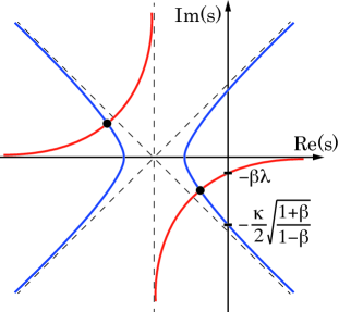
Figure 7: The poles represented by the cross points between two curves.

Note that, as demonstrated above, in general the stability analysis becomes complicated for a complex-coefficient or higher-order transfer function. The Nyquist method Astrom Murray is a very useful graphical tool that can deal with such cases, although an exact stability condition is not available. Another way is a time-domain approach based on the so-called small-gain theorem Zames ; Doyle , that produces a sufficient condition for a feedback-controlled system to be stable; the quantum version of this method DHelon will be useful to test the stability of the controlled feedback amplifier.

Appendix C Phase-conjugating case

The Hermitian conjugate of the second element of Eq. (3) is given by $\tilde{b}_{2}=G_{21}^{*}b_{1}^{\dagger}+G_{22}^{*}b_{2}$. That is, the output $\tilde{b}_{2}$ is the amplified signal of the conjugated input $b_{1}^{\dagger}$, with gain $|G_{21}|$; this is called the phase-conjugating amplification. The feedback control in this case is almost the same as for the phase-preserving amplification. We consider the ideal feedback configuration shown in Fig. 2 (i.e., the noise fields $d_{3},\ldots,d_{6}$ are ignored) and now focus on the auxiliary output $\tilde{b}_{3}=(G_{21}^{\rm(fb)})^{*}b_{1}^{\dagger}+(G_{22}^{\rm(fb)})^{*}b_{4}$. Then the amplification gain is evaluated, in the large amplification limit $|G_{21}|\rightarrow\infty$, as

$$|G_{21}^{({\rm fb})}|=\Big{|}\frac{K_{11}}{1/|G_{21}|-K_{21}G_{22}/|G_{21}|}\Big{|}\rightarrow\Big{|}\frac{K_{11}}{-K_{21}e^{i\theta}}\Big{|}$$

$$\hskip 20.00003pt=\frac{|K_{11}|}{|K_{21}|}=\sqrt{\frac{1}{|K_{21}|^{2}}-1}.$$

In the first line of the above equation, we have used $|G_{22}/G_{21}|^{2}=1+1/|G_{21}|^{2}\rightarrow 1$; also the last equality comes from the unitarity of $K$, i.e., $|K_{11}|^{2}+|K_{21}|^{2}=1$. Therefore, when the original amplification gain is large ($|G_{21}|\gg 1$), the controlled system works as a phase-conjugating amplifier with gain $\sqrt{1/|K_{21}|^{2}-1}>1$. As in the phase-preserving case, this controlled gain is robust compared to the original one $|G_{21}|$.

References

- (1) H. S. Black, Inventing the negative feedback amplifier, IEEE Spectrum 14-12, 55/60 (1977).
- (2) H. S. Black, Stabilized feedback amplifiers (Reprint), Proc. IEEE 72-6, 716/722 (1984).
- (3) R. Mancini, Op Amps for Everyone, Texas Instruments Guide, Technical Report, URL http:// focus.ti.com/lit/an/slod006b/slod006b.pdf (2002).
- (4) J. Bechhoefer, Feedback for physicists: A tutorial essay on control, Rev. Mod. Phys. 77, 783 (2005).
- (5) H. A. Haus and J. A. Mullen, Quantum noise in linear amplifiers, Phys. Rev. 128, 2407 (1962).
- (6) C. M. Caves, Quantum limits on noise in linear amplifiers, Phys. Rev. D 26, 1817 (1982).
- (7) S. L. Braunstein, N. J. Cerf, S. Iblisdir, P. van Loock, and S. Massar, Optimal cloning of coherent states with a linear amplifier and beam splitters, Phys. Rev. Lett. 86, 4938 (2001).
- (8) R. Loudon, O. Jedrkiewicz, S. M. Barnett, and J. Jeffers, Quantum limits on noise in dual input-output linear optical amplifiers and attenuators, Phys. Rev. A 67, 033803 (2003).
- (9) M. Sabuncu, G. Leuchs, and U. L. Andersen, Experimental continuous-variable cloning of partial quantum information, Phys. Rev. A 78, 052312 (2008).
- (10) A. A. Clerk, M. H. Devoret, S. M. Girvin, F. Marquardt, and R. J. Schoelkopf, Introduction to quantum noise, measurement, and amplification, Rev. Mod. Phys. 82, 1155 (2010).
- (11) H. M. Chrzanowski, et al., Measurement-based noiseless linear amplification for quantum communication, Nat. Photonics 8, 333 (2014).
- (12) R. W. Andrews, et al., Bidirectional and efficient conversion between microwave and optical light, Nat. Phys. 10, 321 (2014).
- (13) F. Hudelist, J. Kong, C. Liu, J. Jing, Z. Y. Ou, and W. Zhang, Quantum metrology with parametric amplifier-based photon correlation interferometers, Nat. Commun. 5, 3049 (2014).
- (14) M. Silveri, E Zalys-Geller, M. Hatridge, Z. Leghtas, M. H. Devoret, and S. M. Girvin, Theory of remote entanglement via quantum-limited phase-preserving amplification, arXiv:1507.00732 (2015).
- (15) V. Josse, M. Sabuncu, N. J. Cerf, G. Leuchs, and U. L. Andersen, Universal optical amplification without nonlinearity, Phys. Rev. Lett. 96, 163602 (2006).
- (16) N. Bergeal, et al., Phase-preserving amplification near the quantum limit with a Josephson ring modulator, Nature 465, 64 (2010).
- (17) N. Bergeal, et al., Analog information processing at the quantum limit with a Josephson ring modulator, Nat. Phys. 6, 296 (2010).
- (18) H. Nha, G. J. Milburn, and H. J. Carmichael, Linear amplification and quantum cloning for non-Gaussian continuous variables, New J. Phys. 12, 103010 (2010).
- (19) J. Yoshikawa, Y. Miwa, R. Filip, and A. Furusawa, Demonstration of a reversible phase-sensitive optical amplifier, Phys. Rev. A 83, 052307 (2011).
- (20) C. M. Caves, J. Combes, Z. Jiang, and S. Pandey, Quantum limits on phase-preserving linear amplifiers, Phys. Rev. A 86, 063802 (2012).
- (21) A. Metelmann and A. A. Clerk, Quantum-limited amplification via reservoir engineering, Phys. Rev. Lett. 112, 133904 (2014).
- (22) B. Abdo, et al., Josephson directional amplifier for quantum measurement of superconducting circuits, Phys. Rev. Lett. 112, 167701 (2014).
- (23) A. Metelmann and A. A. Clerk, Nonreciprocal photon transmission and amplification via reservoir engineering, Phys. Rev. X 5, 021025 (2015).
- (24) R. Hamerly and H. Mabuchi, Optical devices based on limit cycles and amplification in semiconductor optical cavities, Phys. Rev. Appl. 4, 024016 (2015).
- (25) R. Slavik, et al., All-optical phase and amplitude regenerator for next-generation telecommunications systems, Nat. Photonics 4, 690 (2010).
- (26) S. Pandey, Z. Jiang, J. Combes, and C. M. Caves, Quantum limits on probabilistic amplifiers, Phys. Rev. A 88, 033852 (2013).
- (27) Z. L.-Dastjerdi, et al., Parametric amplification and phase preserving amplitude regeneration of a 640 Gbit/s RZ-DPSK signal, Opt. Express 21, 25944 (2013)
- (28) H. M. Wiseman and G. J. Milburn, All-optical versus electro-optical quantum-limited feedback, Phys. Rev. A 49, 4110 (1994).
- (29) M. R. James, H. I. Nurdin, and I. R. Petersen, control of linear quantum stochastic systems, IEEE Trans. Autom. Control 53-8, 1787 (2008).
- (30) J. Gough and M. R. James, The series product and its application to quantum feedforward and feedback networks, IEEE Trans. Automat. Contr. 54-11, 2530 (2009).
- (31) R. Hamerly and H. Mabuchi, Advantages of coherent feedback for cooling quantum oscillators, Phys. Rev. Lett. 109, 173602 (2012).
- (32) J. Kerckhoff, et al., Tunable coupling to a mechanical oscillator circuit using a coherent feedback network, Phys. Rev. X 3, 021013 (2013).
- (33) N. Yamamoto, Coherent versus measurement feedback: Linear systems theory for quantum information, Phys. Rev. X 4, 041029 (2014).
- (34) A. Buonanno and Y. Chen, Signal recycled laser-interferometer gravitational-wave detectors as optical springs, Phys. Rev. D 65, 042001 (2002).
- (35) B. Yurke, Optical back-action-evading amplifiers, J. Opt. Soc. Am. B 2-5, 732 (1985).
- (36) Z. Y. Ou, S. F. Pereira, and H. J. Kimble, Realization of the Einstein-Podolsky-Rosen paradox for continuous variables in nondegenerate parametric amplification, Appl. Phys. B 55, 265 (1992).
- (37) C. W. Gardiner and P. Zoller, Quantum Noise (Springer, Berlin, 2004).
- (38) N. J. Cerf and S. Iblisdir, Phase conjugation of continuous quantum variables, Phys. Rev. A 64, 032307 (2001).
- (39) M. Sabuncu, U. L. Andersen, and G. Leuchs, Experimental demonstration of continuous variable cloning with phase-conjugate inputs, Phys. Rev. Lett. 98, 170503 (2007).
- (40) H. W. Bode, Network Analysis and Feedback Amplifier Design (van Nostrand, New York, 1945).
- (41) K. J. Astrom and R. M. Murray, Feedback Systems: An Introduction for Scientists and Engineers (Princeton Univ. Press, 2008).
- (42) A. C. Doherty, S. Habib, K. Jacobs, H. Mabuchi, and S. M. Tan, Quantum feedback control and classical control theory, Phys. Rev. A 62, 012105 (2000).
- (43) H. M. Wiseman and G. J. Milburn, Quantum Measurement and Control (Cambridge Univ. Press, 2009).
- (44) K. Jacobs, Quantum Measurement Theory and its Applications (Cambridge Univ. Press, 2014).
- (45) T. C. Ralph and A. P. Lund, Nondeterministic noiseless linear amplification of quantum systems, in Quantum Communication Measurement and Computing, edited by A. Lvovsky, Proceedings of 9th International Conference, 155/160 (AIP, New York, 2009).
- (46) G. Y. Xiang, T. C. Ralph, A. P. Lund, N. Walk, and G. J. Pryde, Heralded noiseless linear amplification and distillation of entanglement, Nat. Photonics 4, 316 (2010).
- (47) N. A. McMahon, A. P. Lund, and T. C. Ralph, Optimal architecture for a nondeterministic noiseless linear amplifier, Phys. Rev. A 89, 023846 (2014).
- (48) J. M. Courty, F. Grassia, and S. Reynaud, Quantum noise in ideal operational amplifiers, Europhys. Lett. 46, 31 (1999).
- (49) G. Zames, On the input-output stability of time-varying nonlinear feedback systems Part one: Conditions derived using concepts of loop gain, conicity, and positivity, IEEE Trans. Autom. Control 11-2, 228/238 (1966).
- (50) K. Zhou, J. Doyle, and K. Glover, Robust and Optimal Control (Prentice-Hall, Englewood Cliffs, NJ, 1996).
- (51) C. D’Helon and M. R. James, Stability, gain, and robustness in quantum feedback networks, Phys. Rev. A 73, 053803 (2006).