Extreme event statistics of daily rainfall: Dynamical systems approach

Abstract

We analyse the probability densities of daily rainfall amounts at a variety of locations on the Earth. The observed distributions of the amount of rainfall fit well to a $q$-exponential distribution with exponent $q$ close to $q\approx 1.3$. We discuss possible reasons for the emergence of this power law. On the contrary, the waiting time distribution between rainy days is observed to follow a near-exponential distribution. A careful investigation shows that a $q$-exponential with $q\approx 1.05$ yields actually the best fit of the data. A Poisson process where the rate fluctuates slightly in a superstatistical way is discussed as a possible model for this. We discuss the extreme value statistics for extreme daily rainfall, which can potentially lead to flooding. This is described by Fréchet distributions as the corresponding distributions of the amount of daily rainfall decay with a power law. On the other hand, looking at extreme event statistics of waiting times between rainy days (leading to droughts for very long dry periods) we obtain from the observed near-exponential decay of waiting times an extreme event statistics close to Gumbel distributions. We discuss superstatistical dynamical systems as simple models in this context.

I Introduction

The statistical analysis of precipitation data is an interesting problem of major environmental importance masutani ; higgins1 ; higgins2 ; silva . Of particular interest are extreme events of rainfall, which can lead to floodings if a given threshold is exceeded. From a mathematical and statistical point of view, it is natural to apply extreme value statistics to measured rainfall data, but it is not so clear which class of the known extreme value statistics, if any, is applicable, and how the results differ from one spatial location to another. Another interesting quantity to look at is the waiting time between rainy days. Extreme events of waiting times in this context correspond to droughts. So an interesting question is what type of drought statistics is implied by the observed distribution of waiting times between rainfall periods if this is extrapolated to very long waiting times.

In this paper we present a systematic investigation of the probability distributions of the amount of daily rainfall at variety of different locations on the Earth, and of waiting time distributions on a scale of days and hours. Our main result is that the observed distributions of the amount of rainfall are well-fitted by $q$-exponentials, rather than exponentials, which suggests that techniques borrowed from nonextensive statistical mechanics tsallis-book and superstatistics beck-cohen could be potentially useful to better understand the rainfall statistics. An entropic exponent of $q\approx 1.3$ is typically observed. In fact, based on the fact that $q$-exponentials asymptotically decay with a power law, we discuss the corresponding extreme value statistics that is highly relevant in the context of floodings produced by extreme rainfall events. We also investigate the waiting time distribution between rainy events, which is much better described by an exponential, although an entropic exponent close to 1 such as $q\approx 1.05$ seems to give the best fits. We discuss possible dynamical reasons for the occurrence of $q$-exponentials in this context.

One possible reason could be superstatistical fluctuations of a variance parameter or a rate parameter. Let us explain this a bit further. Superstatistical techniques have been discussed in many papers beck-cohen ; swinney ; touchette ; jizba ; chavanis ; frank ; celia ; straeten ; mark ; hanel ; guo ; souza ; tsallis1 ; kaniadakis and they represent a powerful method to model and/or analyse complex systems with two (or more) clearly separated time scales in the dynamics. The basic idea is to consider for the theoretical modelling a superposition of many systems of statistical mechanics in local equilibrium, each with its own local variance parameter $\beta$, and finally perform an average over the fluctuating $\beta$. The probability density of $\beta$ is denoted by $f(\beta)$. Most generally, the parameter $\beta$ can be any system parameter that exhibits large-scale fluctuations, such as energy dissipation in a turbulent flow, or volatility in financial markets. Another possibility is to regard $\beta$ as the rate parameter of a local Poisson process, as done, for example, in briggs . Ultimately all expectation values relevant for the complex system under consideration are averaged over the distribution $f(\beta)$. Many applications have been described in the past, including modelling the statistics of classical turbulent flow prl2001 ; prl2007 ; reynolds ; swinney , quantum turbulence miah , space-time granularity jizba2 , stock price changes straeten , wind velocity fluctuations rapisarda , sea level fluctuations pau1 , infection pathways of a virus itto , migration trajectories of tumour cells metzner , and much more chavanis ; abul-magd ; soby ; briggs ; chen ; cosmic . Superstatistical systems, when integrated over the fluctuating parameter, are effectively described by more general versions of statistical mechanics, where formally the Boltzmann-Gibbs entropy is replaced by more general entropy measures hanel ; souza . The concept can also be generalized to general dynamical systems with slowly varying system parameters, see penrose for some recent rigorous results in this direction.

Our main goal in this paper is to better understand the extreme event statistics of rainfall at various example locations on the Earth. We will start with a careful analysis of experimentally recorded time series of the amount of rainfall measured at a given location, whose probability density is highly relevant to model the corresponding extreme event statistics LLR89 ; EKM97 ; Coles01 ; HF06 ; kantz . Ultimately of course all this rainfall dynamics can be formally regarded as being produced by a highly nonlinear and high-dimensional deterministic dynamical system in a chaotic state, producing the occasional rainfall event, hence it is useful to keep in mind the basic results of extreme event statistics for weakly correlated events as generated by mixing dynamical systems. Recently there has been much activity on the rigorous application of extreme values theory to deterministic dynamical systems LFTV ; FLTV ; FF ; FFT ; FFT2 ; HNT ; HVR ; GHN ; Keller and also to stochastically perturbed ones AFV ; FFTV ; FV1 . A remarkable feature of the dynamical system approach is that there exist some correlations between events, and hence the extreme value theory used to tackle it must account for this correlation going beyond a theory that is just based on sequences of events that are statistically independent. In the superstatistics approach, correlations are also present, due to the fact that parameter changes take place on long time scales, but the relaxation time of the system is short as compared to the time scale of these parameter changes, so that local equilibrium is quickly reached.

What is worked out in this paper is a comparison with experimentally measured rainfall data, to decide which extreme event statistics should be most plausibly applied to various questions related to amount of rainfall and waiting times between rainfall events. Extreme value theory quite generally tells us (under suitable asymptotic independence assumptions) that there are only three possible limit distributions, namely, the Gumbel, Fréchet and Weibull distribution. But are these assumptions of near-independence satisfied for rainfall data, and if yes, which of the above three classes are relevant? This is the subject of this paper. We will also discuss simple deterministic dynamical system models that generate superstatistical processes in this context.

The paper is organized as follows. In Section II we present histograms of rainfall statistics, extracted from experimentally measured time series of rainfall at various locations on the Earth. What is seen is that the probability density of amount of rainfall is very well fitted by $q$-exponentials. We discuss the generalized statistical mechanics foundations of this based on nonextensive statistical mechanics with entropic index $q$, with $q\approx 1.3$. In section III we look at waiting time distributions (on a daily and hourly scale) between rainy episodes. These are observed to be close to exponential functions, similar as for the Poisson process. However, a careful analysis shows that a slightly better fit is again given by $q$-exponentials, but this time with $q$ much closer to 1. A simple superstatistical model for this is discussed in section IV, a Poisson process that has a rate parameter that fluctuates in a superstatistical way. We review standard extreme event statistics in section V and then, in section VI, based on the measured experimental results of rainfall statistics, we develop the corresponding extreme value statistics. In section VII we analyse the ambiguities that arise for the extreme event statistics of waiting times, depending on whether we assume the waiting time distribution is either an exact exponential or a slightly deformed $q$-exponential as produced by superstatistical fluctuations. Finally, in section VIII we describe a dynamical systems approach to superstatistics.

II Daily rainfall amount distributions at various locations

We performed a systematic investigation of time series of rainfall data for 8 different example locations on the Earth (Figs. 1-8). The data are from various publicly available web sites. When doing a histogram of the amount of daily rainfall observed, a surprising feature arises. All distributions are power law rather than exponential. They are well fitted by so-called $q$-exponentials, functions of the form

$$e_{q}(x)=(1+(1-q)x)^{1/(1-q)}$$ (1)

which are well-motivated by generalized versions of statistical mechanics relevant for systems with long-range interactions, temperature fluctuations and multifractal phase space structure tsallis-book ; beck-cohen . Of course the ordinary exponential is recovered for $q\to 1$. Whereas the data of most locations are well fitted by $q\approx 1.3$, Central England and Vancouver have somewhat lower values of $q$ closer to 1.13.

One may speculate what the reason for this power law is. Nevertheless, the formalism of nonextensive statistical mechanics tsallis-book is designed to describe complex systems with spatial or temporal long-range interactions, and $q$-exponentials occur in this formalism as generalized canonical distributions that maximize $q$-entropy

$$S_{q}=\frac{1}{q-1}\sum_{i}(1-p_{i}^{q}),$$ (2)

where the $p_{i}$ are the probabilities of the microstates $i$. Ordinary statistical mechanics is recovered in the limit $q\to 1$, where the $q$-entropy $S_{q}$ reduces to the Shannon entropy

$$S_{1}=-\sum_{i}p_{i}\log p_{i}.$$ (3)

The generalized canonical distributions maximize the $q$-entropy subject to suitable constraints. In our case the constraint is given by the average amount of daily rainfall at a given location. The way rainfall is produced is indeed influenced by highly complex weather systems and condensation processes in clouds, so one may speculate that more general versions of statistical mechanics could be relevant as an effective description. Also for hydrodynamic turbulent systems prl2001 ; swinney and pattern forming systems daniels these generalized statistical mechanics methods have previously been shown to yield a good effective description. The amount of rain falling on a given day is a complicated spatio-temporal stochastic process with intrinsic correlations, as rainy weather often has a tendency to persist for a while, both spatially and temporally. The actual value of $q$ for the observed rainfall statistics reflects characteristic effective properties in the climate and temporal precipitation pattern at the given location. For temperature distributions at the same locations as in Fig.1-8, see yalcin .

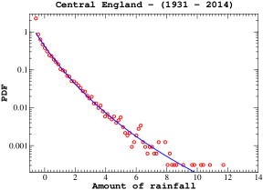
Figure 1: Observed probability distribution of amount of daily rainfall (minus average value) in Central England (red data points). The blue curve is a fit with a $q$-exponential $e_{q}(-x)$. The parameter $q$ is fitted for the various locations. For Central England, $q=1.13$.

 

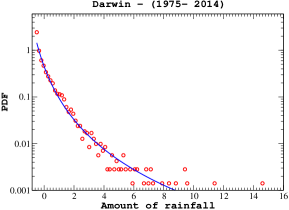
Figure 2: As Fig. 1, but for Darwin ($q=1.30$).

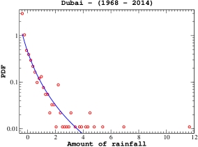
Figure 3: As Fig. 1, but for Dubai ($q=1.30$).

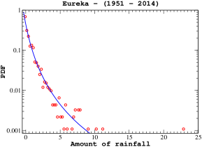
Figure 4: As Fig. 1, but for Eureka ($q=1.30$).

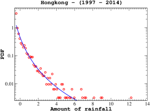
Figure 5: As Fig. 1, but for Hongkong ($q=1.30$).

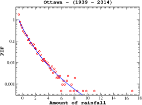
Figure 6: As Fig. 1, but for Ottawa ($q=1.15$).

.

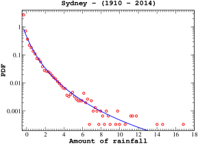
Figure 7: As Fig. 1, but for Sydney ($q=1.25$).

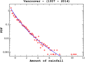
Figure 8: As Fig. 1, but for Vancouver ($q=1.13$).

III Waiting time distributions between rainy days

Another interesting observable that we extracted from the data is the waiting time distribution between rainy episodes. We did this both for a time scale of days and a time scale of hours. A given day is marked as rainy if it rains for some time during that day. The waiting time is then the number of days one has to wait until it rains again, this is a random variable with a given distribution which we can extract from the data. Results for the waiting time distributions are shown in Fig. 9-14. What one observes here is that the distribution is nearly exponential. That means the Poisson process of nearly independent point events of rainy days is a reasonably good model.

At closer inspection, however, one sees that again a slightly deformed $q$-exponential, this time with $q\approx 1.05$, is a better fit of the waiting time distribution. As worked out in the next section, one may explain this with a superstatistical Poisson process, i.e. a Poisson process whose rate parameter – on a long time scale– exhibits fluctuations that are $\chi^{2}$-distributed, with a rather large number of degrees of freedom $n$.

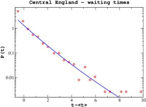
Figure 9: Waiting time distribution between rainy days for Central England (red data points). The blue curve is a fit with a $q$-exponential. For waiting time distributions, the parameter $q$ is much closer to 1 ($q=1.05$ for Central England).

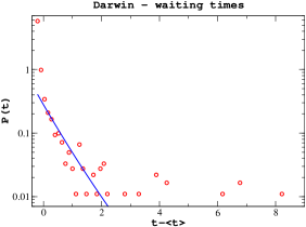
Figure 10: As Fig. 9, but for Darwin ($q=1.05$).

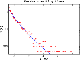
Figure 11: As Fig. 9, but for Eureka ($q=1.10$).

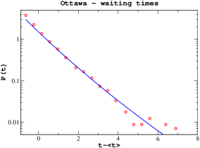
Figure 12: As Fig. 9, but for Ottawa ($q=1.05$).

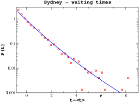
Figure 13: As Fig. 9, but for Sydney ($q=1.06$).

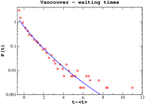
Figure 14: As Fig. 9, but for Vancouver ($q=1.10$).

IV Superstatistical Poisson process

We start with a very simple model for the return time of rainfall events (or extreme rainfall events) on any given time scale. This is to assume that the events follows a Poisson process. For a Poisson process the waiting times are exponentially distributed,

$$p(t|\beta)=\beta\exp(-\beta t).$$

Here, $t$ is the time from one event (peak over threshold) to the next one, and $\beta$ is a positive parameter, the rate of the Poisson process. The symbol $p(t|\beta)$ denotes the conditional probability density to observe a return time $t$ provided the parameter $\beta$ has certain given value.

The key idea of the superstatistics approach beck-cohen ; briggs can be applied to this simple model, thus constructing a superstatistical Poisson process. In this case the parameter $\beta$ is regarded as a fluctuating random variable as well, but these fluctuations take place on a very large time scale. For example, for our rainfall statistics the time scale on which $\beta$ fluctuates may correspond to weeks (different weather conditions) whereas our data base records rainfall events on an hourly basis.

If $\beta$ is distributed with probability density $f(\beta)$, and fluctuates on a large time scale, then one obtains the marginal distribution of the return time statistics as

$$p(t)=\int_{0}^{\infty}f(\beta)p(t|\beta)=\int_{0}^{\infty}f(\beta)\beta\exp(-\beta t).$$ (4)

This marginal distribution is actually what is recorded when we sample histograms of the observational data.

By inferring directly on a simple model for the distribution $f(\beta)$, a more complex model for the return times can be derived without much technical complexity. For example, consider that there are $n$ different Gaussian random variables $X_{i},i=1,\dots,n$, that influence the dynamics of the intensity parameter $\beta$ as a random variable. We may thus assume as a very simple model that $\beta=\sum_{i=1}^{n}X_{i}^{2}$ with $E(X_{i})=0$ and $E(X_{i}^{2})\neq 0$. Then the probability density of $\beta$ is given by a $\chi^{2}$-distribution:

$$f(\beta)=\frac{1}{\Gamma(n/2)}\left(\frac{n}{2\beta_{0}}\right)^{n/2}\beta^{n/2-1}\exp\left(\frac{n\beta}{2\beta_{0}}\right),$$

where $n$ is the number of degrees of freedom and $\beta_{0}$ is a shape parameter that has the physical meaning of being the average of $\beta$ formed with the distribution $f(\beta)$.

The integral (4) is easily evaluated and one obtains the $q$-exponential distribution:

$$p(t)\sim(1+b(q-1)t)^{1/(1-q)},$$

where $q=1+2/(n+2)$ and $b=2\beta_{0}/(2-q)$.

To sum up, this model generates $q$-exponential distributions by a simple mechanism, fluctuations of a rate parameter $\beta$. Typical $q$-values obtained in our fits are $q=1.3$ for rainfall amount and $q=1.05$ for waiting time between rainfall events.

V Extreme value theory for stationary processes

Classic extreme value theory is concerned with the probability distribution of unlikely events. Given a stationary stochastic process $X_{1},X_{2},\dots$, consider the random variable $M_{n}$ defined as the maximum over the first $n$-observations:

$$M_{n}=\max(X_{1},\dots,X_{n}).$$ (5)

In many cases the limit of the random variable $M_{n}$ may degenerate when $n\rightarrow\infty$. Analogously to central limit laws for partial sums, the degeneracy of the limit can be avoided by considering a rescaled sequence $a_{n}(M_{n}-b_{n})$ for suitable normalising values $a_{n}\geq 0$ and $b_{n}\in\mathbb{R}$. Indeed, extreme value theory studies the existence of normalising values such that

$$P\left(a_{n}\left(M_{n}-b_{n}\right)\leq x\right)\rightarrow G\left(x\right).$$ (6)

as $n\rightarrow\infty$, with $G(x)$ a non-degenerate probability distribution.

Two cornerstones in Extreme Value Theory are the Fisher-Tippet Theorem fisher and the Gnedenko Theorem gnedenko . The former asserts that if the limiting distribution $G$ exist, then it must be either one of three possible types, whereas the latter theorem gives necessary and sufficient conditions for the convergence of each of the types. A third cornerstone in Extreme Value Theory are the Leadbetter conditions Leadbetter74 ; LLR89 . These are a kind of weak asymptotic independence conditions, under which the two previous theorems generalize to stationary stochastic series satisfying them. Let us review these results in somewhat more detail.

In the case where the process $X_{i}$ is independent identically distributed (i.i.d.) the Fisher-Tippett Theorem states that if $X_{1},X_{2},\dots$ is i.i.d. and there exist sequences $a_{n}\geq 0$ and $b_{n}\in\mathbb{R}$ such that the limit distribution $G$ is non-degenerate, then it belongs to one of the following types:

Type I :

$G(x)=\exp\left(-e^{-x}\right)$ for $x\in\mathbb{R}$. This distribution is known as the Gumbel extreme value distribution (e.v.d.).

Type II :

$G(x)=\exp\left(-x^{-\alpha}\right)$, for $x>0$; $G(x)=0$, otherwise; where $\alpha>0$ is a parameter. This family of distributions is known as the Fréchet e.v.d.

Type III:

$G(x)=\exp\left(-(-x)^{\alpha}\right)$, for $x\leq 0$; $G(x)=1$, otherwise; where $\alpha>0$ is a parameter. This family is known as the Weibull e.v.d.

A further extension of this result is the Gnedenko Theorem, which provides a characterization of the convergence in each of these cases. Let $X_{1},X_{2},\dots$ be an i.i.d. stochastic process and let $F$ be its cumulative distribution function. Consider $x_{M}=\sup\{x|\,F(x)<1\}$. The following conditions are necessary and sufficient for the convergence to each type of e.v.d.:

Type I:

There exists some strictly positive function $h(t)$ such that $\lim_{t\rightarrow x_{M}^{-}}\frac{1-F(t+xh(t))}{1-F(t)}=e^{-x}$ for all real $x$;

Type II:

$x_{M}=+\infty$ and $\lim_{t\rightarrow\infty}\frac{1-F(tx)}{1-F(t)}=x^{-\alpha}$, with $\alpha>0$, for each $x>0$;

Type III:

$x_{M}<\infty$ and $\lim_{t\rightarrow 0}\frac{1-F(x_{M}-tx)}{1-F(x_{M}-t)}=x^{\alpha}$, with $\alpha>0$, for each $x>0$.

This result implies that the extremal type is completely determined by the tail behaviour of the distribution $F(x)$.

VI Extreme event statistics for exponential and q-exponential distributions

The rainfall data were well described by $q$-exponentials, but waiting time distributions were observed to be close to ordinary exponentials, with $q$ only deviating by a small amount from 1. Let us now discuss the differences in extreme value statistics that arise from theses different distributions.

In the case where $X$ is distributed as an ordinary exponential function with parameter $\lambda$, we have

$$1-F(t)=\left\{\begin{array}[]{rcl}\exp(-\lambda t)&\text{ if }&t>0\\ 1&\text{ if }&t<0.\end{array}\right.$$ (7)

It is not difficult to check that the exponential distribution belongs to the Gumbel domain of attraction. In other words, the extreme events associated to the exponential distribution will be Gumbel distributed.

Recall that the $q$-exponential function is defined as

$$\exp_{q}(t):=\left[1+(1-q)t\right]^{1/(1-q)},$$

with $1\leq q<2$. A random variable $X$ is $q$-exponential distributed (with parameter $\lambda$) if its density function is equal to $(2-q)\lambda\exp_{q}(-\lambda x)$. In such a case, its hazard function is

$$1-F(t)=\left\{\begin{array}[]{rcl}\exp_{q^{\prime}}\left(-\lambda t/q^{\prime}\right)&\text{ if }&t>0\\ 1&\text{ if }&t<0.\end{array}\right.$$ (8)

where $q^{\prime}=1/(2-q)$.

Using the Gnedenko theorem if follows that the $q$-exponential distribution belongs to the Fréchet domain of attraction. In this case the shape parameter of the Fréchet distribution $\alpha$ is equal to $\frac{2-q}{q-1}$.

VII Model uncertainty

Extremely large waiting times for rainfall events correspond to droughts. Clearly, it is interesting to extrapolate our observed waiting time distributions to very large time scales. However, in Section III we saw that in most cases it is difficult to discern if the waiting time distribution is that of a Poisson process, distributed as an exponential, or if it is a $q$-exponential with $q$ close to one. This can make a huge difference for extreme value statistics. The aim of this section is to assess the impact of choosing one or the other model.

Consider $k$ a constant and $X$ a random variable modelled either by an exponential or a $q$-exponential. To normalize the problem, we can scale our analysis in terms of the mean. In other words, we look at the probability of $X$ being bigger than a multiple, say $k$-times, the mean of $X$.

If $X$ is distributed like an exponential with parameter $\lambda$, its mean is equal to $1/\lambda$ and its hazard function is given by (7). Then it is easy to check that

$$P(X>kE(X))=\exp\left(-k\right).$$

On the other hand, if $X$ is distributed like a $q$-exponential with parameter $\lambda$, its mean is equal to $1/\lambda(3-2q)$ (provided $1\leq q<3/2$) and its hazard function is given by (8). In this case we have

$$P(X>kE(X))=\exp_{q^{\prime}}\left(-\frac{2-q}{3-2q}k\right).$$

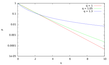
Figure 15: Horizontal axis: Multiple $k$ of the mean, vertical axis: probability $P$ for an event at that level.

Recall that the exponential distribution can be understood as the limit of the $q$-exponential as $q$ goes to $1$. This is also true for the probability above, which converges to $\exp\left(-k\right)$ as $q$ goes to $1$. In Fig 15 we plotted the probability of an event of level $k$ for different values of $q$. For instance the probability of having an observation bigger than $5$ times the mean is $0.0068$ for $q=1$, $0.0095$ when $q=1.05$ and $0.026$ when $q=1.3$. When we look at the probability of an observation bigger than $10$ the mean, it is $0.000045$, $0.00023$ and $0.0068$ respectively. Apparently, the predicted drought statistics is very different choosing either the value $q=1$ or the very similar value $q=1.05$ for the observed waiting time distribution. This illustrates the general uncertainty in model building for extreme rainfall and drought events pau2 .

VIII Dynamical systems approach

Ultimately, the weather and rainfall events at a given location can be regarded as being produced by a very high-dimensional deterministic dynamical system exhibiting chaotic properties. It is therefore useful to extend the superstatistics concept to general dynamical systems, following similar lines of arguments as in the recent paper penrose .

The basic idea here is that one has a given dynamics (which, for simplicity, we take to be a discrete mapping $f_{a}:\Omega\to\Omega$ on some phase space $\Omega$) which depends on some control parameter $a$. If $a$ is changing on a large time scale, much larger than the local relaxation time determined by the Perron-Frobenius operator of the mapping, then this dynamical system with slowly changing control parameter will ultimately generate a superposition of invariant densities for the given parameter $a$. Similarly, if we can calculate return times to certain particular regions of the phase space for a given parameter $a$, then in the long term the return time distribution will have to be formed by taking an average over the slowly varying parameter $a$. Clearly, the connection to the previous sections is that a rainfall event corresponds to the trajectory of the dynamical system being in a particular subregion of the phase space $\Omega$, and the control parameter $a$ corresponds to the parameter $\beta$ used in the previous sections.

Let us consider families of maps $f_{a}$ depending on a control parameter $a$. These can be a priori arbitrary maps in arbitrary dimensions, but it is useful to restrict the analysis to mixing maps and assume that an absolutely continuous invariant density $\rho_{a}(x)$ exists for each value of the control parameter $a$. The local dynamics is

$$x_{n+1}=f_{a}(x_{n}).$$ (9)

We allow for a time dependence of $a$ and study the long-term behavior of iterates given by

$$x_{n}=f_{a_{n}}\circ f_{a_{n-1}}\circ\ldots f_{a_{1}}(x_{0}).$$ (10)

Clearly, the problem now requires the specification of the sequence of control parameters $a_{1},\ldots,a_{n}$ as well, at least in a statistical sense. One possibility is a periodic orbit of control parameters of length $L$. Another possibility is to regard the $a_{j}$ as random variables and to specify the properties of the corresponding stochastic process in parameter space. This then leads to a distribution of parameters $a$.

In general, rapidly fluctuating parameters $a_{j}$ will lead to a very complicated dynamics. However, there is a significant simplification if the parameters $a_{j}$ change slowly. This is the analogue of the slowly varying temperature parameters in the superstatistical treatment of nonequilibrium statistical mechanics beck-cohen . The basic assumption of superstatistics is that an environmental control parameter $a$ changes only very slowly, much slower than the local relaxation time of the dynamics. For maps this means that significant changes of $a$ occur only over a large number $T$ of iterations. For practical purposes one can model this superstatistical case as follows: One keeps $a_{1}$ constant for $T$ iterations ($T>>1$), then switches after $T$ iterations to a new value $a_{2}$, after $T$ iterations one switches to the next values $a_{3}$, and so on.

One of the simplest examples is a period-2 orbit in the parameter space. That is, we have an alternating sequence $a_{1},a_{2}$ that repeats itself, with switching between the two possible values taking place after $T$ iterations. This case was given particular attention in penrose , and rigorous results were derived for special types of maps where the invariant density $\rho_{a}$ as a function of the parameter $a$ is under full control, so-called Blaschke products.

Here we discuss two important examples, which are of importance in the context of the current paper, namely how to generate (in a suitable limit) a superstatistical Langevin process, as well as a superstatistical Poisson process, using strongly mixing maps.

Example 1 Superstatistical Langevin-like process We take for $f_{a}$ a map of linear Langevin type roep ; dyna . This means $f_{a}$ is a 2-dimensional map given by a skew product of the form

$$x_{n+1} = g(x_{n})$$ (11)

$$y_{n+1} = e^{-a\tau}y_{n}+\tau^{1/2}(x_{n}-\bar{g})$$ (12)

Here $\bar{g}$ denote the average of iterates of $g$. It has been shown in roep that for $\tau\to 0$, $t=n\tau$ finite this deterministic chaotic map generates a dynamics equivalent to a linear Langevin equation vKa , provided the map $g$ has the so-called $\varphi$-mixing property billingsley , and regarding the initial values $x_{0}\in[0,1]$ as a smoothly distributed random variable. Consequently, in this limit the variable $y_{n}$ converges to the Ornstein-Uhlenbeck process roep ; dyna and its stationary density is given by

$$\rho_{\beta}(y)=\sqrt{\frac{\beta}{2\pi}}e^{-\frac{1}{2}\beta y^{2}}$$ (13)

The variance parameter $\beta$ of this Gaussian depends on the map $g$ and the damping constant $a$. If the parameter $a$ changes on a very large time scale, much larger than the local relaxation time to equilibrium, one expects for the long-term distribution of iterates a mixture of Gaussian distributions with different variances $\beta^{-1}$. For example, a period 2 orbit of parameter changes yields a mixture of two Gaussians

$$p(y)=\frac{1}{2}\left(\sqrt{\frac{\beta_{1}}{2\pi}}e^{-\frac{1}{2}\beta_{1}y^{2}}+\sqrt{\frac{\beta_{2}}{2\pi}}e^{-\frac{1}{2}\beta_{2}y^{2}}\right).$$ (14)

Generally, for more complicated parameter changes on the long time scale $T$, the long-term distribution of iterates $y_{n}$ will be given by a mixture of Gaussians with a suitable weight function $h(\beta)$ for $\tau\to 0$:

$$p(y)\sim\int d\beta\;h(\beta)e^{-\frac{1}{2}\beta y^{2}}$$ (15)

This is just the usual form of superstatistics used in statistical mechanics, based on a mixture of Gaussians with fluctuating variance with a given weight function beck-cohen . Thus for this example of skew products the superstatistics of the map $f_{a}$ reproduces the concept of superstatistics in nonequilibrium statistical mechanics, based on the Langevin equation. In fact, the map $f_{a}$ can be regarded as a possible microscopic dynamics underlying the Langevin equation. The random forces pushing the particle left and right are in this case generated by deterministic chaotic map $g$ governing the dynamics of the variable $x_{n}$. Generally it is possible to consider any $\varphi$-mixing map here roep . Based on functional limit theorems, one can prove equivalence with the Langevin equation in the limit $\tau\to 0$.

We note in passing that if the mixing property is not satisfied, then of course much more complicated probability distributions are expected for sums of iterates of a given map $g$. Numerical evidence has been presented that in this case often $q$-Gaussians with $q>1$ are observed tir1 ; tir2 ; tir3 .

Example 2 Superstatistical Poisson-like process

Take $f_{a}:\Omega\to\Omega$ to be a strongly mixing map, for example the binary shift map $f_{a}(x)=2x\mod 1$ on the interval $\Omega=[0,1]$. Consider a very small subset of the phase space of size $\epsilon$, say $I_{\epsilon}=[1-\epsilon,1]$ and a generic trajectory of the binary shift map for a generic initial value $x_{0}=\sum_{i=1}^{\infty}\sigma_{i}2^{-i}$, where $\sigma_{i}\in\{0,1\}$ are the digits of the binary expansion of the initial value $x_{0}$. We define a ‘rainfall’ event to happen if this trajectory enters $I_{\epsilon}$ (of course, for true rainfall events the dynamical system is much more complicated and lives on a much higher-dimensional phase space). It is obvious that the above sequence of events follows Poisson-like statistics, as the iterates of the binary shift map are strongly mixing, which means asymptotic statistical independence for a large number of iterations. Indeed between successive visits of the very small interval $I_{\epsilon}$, there is a large number of iterations and hence near-independence. Hence the binary shift map generates a very good approximation of the Poisson process for small enough $\epsilon$, and the waiting time distribution between events is exponential.

We may of course also look at a more complicated system $f_{a}$, where we iterate a strongly mixing map $f_{a}$ which depends on a parameter $a$, and where the invariant density $\rho_{a}$ of the map $f_{a}$ depends on the control parameter in a nontrivial way. Examples are Blaschke products, studied in detail in penrose . If the parameter $a$ varies on a large time scale, so does the probability $p_{\epsilon}=\int_{I_{\epsilon}}\rho_{a}(x)dx$ of iterates to enter the region $I_{\epsilon}$, and hence the rate parameter of the above Poisson-like process will also vary. The result is a superstatistical Poisson-like process, generated by a family of deterministic chaotic mappings $f_{a}$. In this way we can build up a formal mathematical framework to dynamically generate superstatistical Poisson processes.

IX Conclusion

We started this paper with experimental observations: The probability densities of daily rainfall amounts at a variety of locations on the Earth are not Gaussian or exponentially distributed, but follow an asymptotic power law, the $q$-exponential distribution. The corresponding entropic exponent $q$ is close to $q\approx 1.3$. The waiting time distribution between rainy episodes is observed to be close to an exponential distribution, but again a careful analysis shows that a $q$-exponential is a better fit, this time with $q$ close to 1.05. We discussed the corresponding extreme value distributions, leading to Gumbel and Fréchet distributions. We made contact with a very important concept that is borrowed from nonequilibrium statistical mechanics, the superstatistics approach, and pointed out how to generalize this concept to strongly mixing mappings that can generate Langevin-like and Poisson-like processes for which the corresponding variance or rate parameter fluctuates in a superstatistical way. Of course rainfall is ultimately described by a very high dimensional and complicated spatially extended dynamical system, but simple model systems as discussed in this paper may help.

References

- (1) Silva, V.B.S; Kousky, V.E.; Higgins R.W. Daily Precipitation Statistics for South America: An Intercomparison between NCEP Reanalyses and Observations. Journal of Hydrometeorology 2011 12(1), 101-117.
- (2) Higgins, R.W.; Silva, V.B.S.; Shi, W.; Larson, J. Relationships between Climate Variability and Fluctuations in Daily Precipitation overthe United States Journal of Climate 2007 20(14), 3561-3579.
- (3) Higgins, R. W.; Schemm, J. E.; Shi, W.; Leetmaa, A. Extreme precipitation events in the western United States related to tropical forcing. Journal of Climate 2007 13(4), 793-820.
- (4) Masutani, M.; Leetmaa, A. Dynamical mechanisms of the 1995 California floods. Journal of Climate 1999 12(11), 3220-3236.
- (5) Tsallis, C. Introduction to nonextensive statistical mechanics. Springer: New York, 2009.
- (6) Beck, C.; Cohen, E.G.D. Superstatistics. Physica A: Statistical Mechanics and its Applications 2003 322, 267-275.
- (7) Beck, C.; Cohen, E. G.; Swinney, H. L. From time series to superstatistics. Physical Review E 2005 72(5), 056133.
- (8) Touchette, H.; Beck, C. Asymptotics of superstatistics. Physical Review E 2005 71(1), 016131.
- (9) Jizba, P.; Kleinert, H. Superpositions of probability distributions. Physical Review E 2008 78(3), 031122.
- (10) Chavanis, P.H. Quasi-stationary states and incomplete violent relaxation in systems with long-range interactions. Physica A: Statistical Mechanics and its Applications 2006 365(1), 102-107.
- (11) Frank, S.A.; Smith, D. E. Measurement invariance, entropy, and probability. Entropy 2010 12(3) 289-303.
- (12) Anteneodo, C.; Duarte Queiros, S.M.; Statistical mixing and aggregation in Feller diffusion. Journal of Statistical Mechanics: Theory and Experiment 2009 10, P10023.
- (13) Van der Straeten, E.; Beck, C. Superstatistical fluctuations in time series: Applications to share-price dynamics and turbulence. Physical Review E 2009 80(3), 036108.
- (14) Mark, C.; Metzner, C.; Fabry, B. Bayesian inference of time varying parameters in autoregressive processes. arXiv:1405.1668.
- (15) Hanel, R.; Thurner, S.; Gell-Mann, M. Generalized entropies and the transformation group of superstatistics. PNAS 2011 108(16) 6390-6394.
- (16) Guo, J.-L.; Suo, Q. Upper Entropy Axioms and Lower Entropy Axioms for Superstatistics. arXiv:1406.4124.
- (17) Tsallis, C.; Souza, A.M.C. Constructing a statistical mechanics for Beck-Cohen superstatistics. Physical Review E 2003 67(2) 026106.
- (18) Tsallis, C. Possible generalization of Boltzmann-Gibbs statistics. Journal of Statistical Physics 1988 52(1-2), 479-487.
- (19) Kaniadakis, G.; Lissia, M.; Scarfone, A.M. Two-parameter deformations of logarithm, exponential, and entropy: A consistent framework for generalized statistical mechanics. Physical Review E 2005 71(4), 046128.
- (20) Briggs, K.; Beck, C. Modelling train delays with q-exponential functions. Physica A: Statistical Mechanics and its Applications 2007 378(2), 498-504.
- (21) Beck, C. Dynamical foundations of nonextensive statistical mechanics. Physical Review Letters 2001 87(18), 180601.
- (22) Reynolds, A. M. Superstatistical mechanics of tracer-particle motions in turbulence. Physical Review Letters 2003 91(8), 084503.
- (23) Beck, C. Statistics of three-dimensional Lagrangian turbulence. Physical Review Letters 2007 98(6), 064502.
- (24) Beck, C.; Miah, S. Statistics of Lagrangian quantum turbulence. Physical Review E 2013 87(3), 031002(R).
- (25) Jizba, P.; Scardigli, F. Special relativity induced by granular space. Eur. Phys. J. C 2013 73, 2491.
- (26) Rizzo, S. and Rapisarda, A. Environmental atmospheric turbulence at Florence airport. AIP Conf. Proc. 2004 742, 176.
- (27) Rabassa, P.; Beck, C. Superstatistical analysis of sea-level fluctuations. Physica A: Statistical Mechanics and its Applications 2015 417, 18-28.
- (28) Itto, Y. Heterogeneous anomalous diffusion in view of superstatistics. Physics Letters A 2014 378(41), 3037-3040.
- (29) Metzner C.; Mark, C.; Steinwachs, J.; Lautscham,L.; Stadler,F; Fabry, B. Superstatistical analysis and modelling of heterogeneous random walks, Nature Communications 2015 6:7516
- (30) Leon Chen, L.; Beck, C. A superstatistical model of metastasis and cancer survival. Physica A: Statistical Mechanics and its Applications 2008 387(13), 3162-3172.
- (31) Abul-Magd, A. Y.; Akemann, G.; Vivo, P. Superstatistical generalizations of Wishart-Laguerre ensembles of random matrices. Journal of Physics A: Mathematical and Theoretical 2009 42(17), 175207.
- (32) Beck, C. Generalized statistical mechanics of cosmic rays. Physica A: Statistical Mechanics and its Applications 2004 331(1), 173-181.
- (33) Sobyanin, D. N. Hierarchical maximum entropy principle for generalized superstatistical systems and Bose-Einstein condensation of light. Physical Review E 2012 85(6), 061120.
- (34) Penrose, C.; Beck, C. Superstatistics of Blaschke products. Dynamical Systems 2016 31(1), 89-105.
- (35) Leadbetter, M. R., Lindgren, G., Rootzén, H., Extremes and related properties of random sequences and processes. Springer, 1989.
- (36) Embrechts, P., Klüpperberg, C., Mikosch, T., Modelling Extremal Events. Springer, 1997.
- (37) Coles, S., An Introduction to Statistical Modeling of Extreme Values. Springer, 2001.
- (38) de Haan, L., Ferreira, A., Extreme Value Theory: An Introduction. Springer, 2006.
- (39) Santhanam, M. S.; Kantz, H. Return interval distribution of extreme events and long-term memory. Physical Review E 2008 78(5), 051113.
- (40) Lucarini, V.; Faranda, D.; Turchetti, G.; Vaienti, S. Extreme value theory for singular measures. Chaos: An Interdisciplinary Journal of Nonlinear Science 2012 22(2), 023135.
- (41) Faranda, D.; Lucarini, V.; Turchetti, G.; Vaienti, S. Numerical convergence of the block-maxima approach to the Generalized Extreme Value distribution. Journal of Statistical Physics 2011 145(5), 1156-1180.
- (42) Freitas, A. C. M.; Freitas, J. M. On the link between dependence and independence in extreme value theory for dynamical systems. Statistics & Probability Letters 2008 78(9), 1088-1093.
- (43) Freitas, A. C. M.; Freitas, J. M.; Todd, M. Extreme value laws in dynamical systems for non-smooth observations. Journal of Statistical Physics 2011 142(1), 108-126.
- (44) Freitas, A. C. M.; Freitas, J. M.; Todd, M. The extremal index, hitting time statistics and periodicity. Advances in Mathematics 2012 231(5), 2626-2665.
- (45) Holland, M.; Nicol, M.; Török, A. Extreme value theory for non-uniformly expanding dynamical systems. Transactions of the American Mathematical Society 2012 364(2), 661-688.
- (46) Holland, M. P.; Vitolo, R.; Rabassa, P.; Sterk, A. E.; Broer, H. W. Extreme value laws in dynamical systems under physical observables. Physica D: Nonlinear Phenomena 2012 241(5), 497-513.
- (47) Gupta, C.; Holland, M.; Nicol, M. Extreme value theory and return time statistics for dispersing billiard maps and flows, Lozi maps and Lorenz-like maps. Ergodic Theory and Dynamical Systems 2011 31(05), 1363-1390.
- (48) Keller, G. Rare events, exponential hitting times and extremal indices via spectral perturbation. Dynamical Systems 2012 27(1), 11-27.
- (49) Aytaç, H.; Freitas, J. M.; Vaienti, S. Laws of rare events for deterministic and random dynamical systems. Transactions of the American Mathematical Society 2015 367(11), 8229-8278.
- (50) Faranda, D.; Freitas, J. M.; Lucarini, V.; Turchetti, G.; Vaienti, S. Extreme value statistics for dynamical systems with noise. Nonlinearity 2013 26(9), 2597.
- (51) Faranda, D.; Vaienti, S. Extreme Value laws for dynamical systems under observational noise. Physica D: Nonlinear Phenomena 2014 280, 86-94.
- (52) Daniels, K. E.; Beck, C.; Bodenschatz, E. Defect turbulence and generalized statistical mechanics. Physica D: Nonlinear Phenomena 2004 193(1), 208-217.
- (53) Yalcin, G. C.; Beck, C. Environmental superstatistics. Physica A: Statistical Mechanics and its Applications 2013 392(21), 5431-5452.
- (54) Fisher, R. A.; Tippett, L. H. C. Limiting forms of the frequency distribution of the largest or smallest member of a sample. Mathematical Proceedings of the Cambridge Philosophical Society 1928 (Vol. 24, No. 02, pp. 180-190). Cambridge University Press.
- (55) Gnedenko, B. Sur la distribution limite du terme maximum d’une serie aleatoire. Annals of Mathematics 1943 44(3), 423-453.
- (56) Leadbetter, M. R. On extreme values in stationary sequences. Zeitschrift für Wahrscheinlichkeitstheorie und verwandte Gebiete 1974 28(4), 289-303.
- (57) Rabassa, P.; Beck, C. Extreme value laws for superstatistics. Entropy 2014 16(10), 5523-5536.
- (58) Beck C.; Roepstorff G. From dynamical systems to the Langevin equation. Physica A: Statistical Mechanics and its Applications 1987 145, 1-14.
- (59) Beck C. Dynamical systems of Langevin type. Physica A: Statistical Mechanics and its Applications 1996 233, 419-440.
- (60) van Kampen, N.G. Stochastic processes in physics and chemistry. North-Holland, Amsterdam 1982
- (61) Billingsley P. Convergence of probability measures. Wiley, New York 1968
- (62) Tirnakli, U.; Beck, C.; Tsallis, C. Central limit behavior of deterministic dynamical systems. Physical Review E 2007 75, 040106(R).
- (63) Tirnakli, U.; Tsallis, C.; Beck, C. Closer look at time averages of the logistic map. Physical Review E 2009 79, 056209.
- (64) Tirnakli, U.; Borges, E.P. The standard map: From Boltzmann-Gibbs statistics to Tsallis statistics. arXiv:1501.02459.