The role of the Havriliak-Negami relaxation in the description of local structure of Kohlrausch’s function in the frequency domain. Part II

Abstract

Two new sets of models for describing compactly the Fourier Transform of Kohlrausch-Williams-Watts, both based on the adiabatic variation of parameters of a double Havriliak-Negami approximation along the whole interval of frequencies, are presented. One of them is relying, obviously, on the use of a well-behaved-pair of patches of the mentioned type of approximants, $\mathcal{A}p_{2}HN(\omega)$. The other is obtained by altering the simple functions $HN(\omega)$ and making dissimilar the couple. They are proposed the guidelines of a new and systematic approach with extended Havriliak-Negami functions which is global, (non local), and of constant parameters. The latter at the cost of a more complicated dependency with the low frequencies than $1+(i\omega\tau_{HN})^{\alpha}$.

¹Instituto de Física Fundamental, IFF-CSIC, Serrano 123, Madrid ES-28006, Spain

²Departamento de Química, Facultad de Ciencias del Mar, ULPGC, Campus Universitario de Tafira, Las Palmas de G. Canaria ES-35017, Spain

Introduction

To the extent that the object of study of soft matter and fluids has been passing from simple polar liquids to polymer, glasses and quasi-amorphous materials, the phenomenology of rheological, or dielectric, relaxations of physical systems has become increasingly complicated. And it is not only that several types of those relaxations are superposed along frequency space making difficult to distinguish among them, but that employed functional form evolves from an easy one as Debye [1], $\frac{1}{1+i\omega}$, to other more complex as Havriliak-Negami [2, 3], $\frac{1}{(1+(i\omega)^{\alpha})^{\gamma}}$, after experimenting with intermediate stages as Cole-Cole [4], $\frac{1}{1+(i\omega)^{\alpha}}$, and Cole-Davidson [5], $\frac{1}{(1+i\omega)^{\gamma}}$.

Simultaneously something similar happens in time description while we consider the different temporal scales implied, so certain habit to model, –imposed by the mentioned physical phenomena and the discriminatory ability of experimental equipment–, shows a methodological exhaustion. In this sense any testing for the use of new relaxation functions, giving account of the novel experimental records, is fully justified [6, 7].

However, as has been quoted previously ([8, 9, 10, 11, 12, 13, 14, 15]), the swapping from one functional space to the other still continues to be hard, often drawing upon, the researcher, efficient numerical methods to perform such devious change [16, 17, 18, 19].

Nevertheless it turns to be sometimes unsatisfactory this capability for blind calculations as it does not provide many times of a general view allowing for the interpretation and identification of these models whose available information is fragmentary or incomplete. In this sense a catalogue for formulae linking frequency and time realms [14], is a precious help while are appraised significant system parameters. Besides it is also an essential partner of the numerical analysis to bound errors and expose constructs [19, 20, 21], both characteristics of computer techniques.

We already have shown as a set of Weibull distributions [22], ($\beta t^{\beta-1}\exp-t^{\beta}$, $0<\beta\leq 2$), in Fourier space, $\psi_{\beta}(\omega)$, admit a good approximate description by sums of Havriliak-Negami functions [23, 24, 25]. Additionally in a precedent paper to this work [25], it is established the local character of the approximation and how, with slight variation of the parameters $\{\alpha_{1,2},\gamma_{1,2},\tau_{1,2},\lambda\}$ with frequency $\omega$, $Ap_{2}HN$ can describe a perfect fit with the objective function, $\psi_{\beta}$. Such adiabatic behavior is commonly misunderstood as an argument against the approximation by means of basic relaxation functions as Havriliak-Negami. This fact it is best interpreted as the need for a wider family of relaxations with a known local portrayal.

Thus in this job we will focus on taking advantage of such “local” information to build “global” functions that ameliorate the preceding approximation in the whole range of frequencies, $[0,\infty)$. Also the relative error of all proposed models in the present and previous report [25] is depicted and tested against the real data obtained from Fourier integrals.

1 Uncommon approaches

1.1 The global two-term approximant: version with an atlas

In short we have constructed two approximants of type [25],

$$\mathcal{A}p_{2}HN_{\alpha,\gamma,\tau,\lambda}(\omega)=\sum_{s=1}^{2}\frac{\lambda_{s}}{(1+(i\tau_{s}\omega)^{\alpha_{s}})^{\gamma_{s}}},$$ (1)

($\lambda_{1}+\lambda_{2}=1$), for two different overlapping intervals $\nu\in[0,500.0005]$ and $\nu\in[1.00,10^{12}]$, (or $\nu\in[1.00,10^{7}]$ if $\beta>1$). Besides if we consider how the relative error between moduli of approximant and function behaves as frequency varies, (i.e. it stabilizes at an almost constant value never greater than 0.2% for high frequencies and $0<\beta\leq 2$), the upper bound of second interval can be extended without a big amount of error to an unlimited frequency. It means that there are two charts $(\mathcal{A}p_{2,l}HN(\omega),\Omega_{l})$ and $(\mathcal{A}p_{2,h}HN(\omega),\Omega_{h}^{*})$ with $\Omega_{l}\equiv 2\pi\times$ $(0,500.0005)$ and $\Omega_{h}^{*}\equiv 2\pi\times$ $(1,\infty)$ that reconstruct in an acceptable way the function $\psi_{\beta}(\omega)$ in the whole interval $(0,\infty)$, plus the value at $\psi_{\beta}(0)=1$ as an imposed condition.

Now, all that is needed to obtain a global solution is a way to merge both charts without overlaps, following a standard procedure. We will resort to an smooth, and monotonously increasing, function defined as:

$$\mathcal{W}_{i,s}(\omega)=\begin{cases}\begin{array}[]{cc}0&:\\ (0,1)&:\\ 1&:\end{array}&\begin{array}[]{c}\omega\leq\omega_{i}\\ \omega_{i}<\omega<\omega_{s}\\ \omega_{s}\leq\omega\end{array}\end{cases},$$

with $\omega_{i}$ and $\omega_{s}$ chosen arbitrarily. So starting from locally adjusted functions which are properly selected it is possible to write a suitable approximation to function $\psi_{\beta}$, in the whole interval $[0,\infty)$, as:

$$\mathcal{A}p_{2}HN(\omega)=\mathcal{A}p_{2,l}HN(\omega)\times(1-\mathcal{W}_{i,s})+\mathcal{A}p_{2,h}HN(\omega)\times\mathcal{W}_{i,s}.$$ (2)

With our particular choice $\omega_{i}=2\pi$ and $\omega_{s}=4\pi$, (or $\omega_{s}=2.2\pi$ if $\beta>1$), we have finally laid down a global surrogate of Havriliak-Negami type for the Fourier Transform of Weibull function $\psi_{\beta}(\omega)$, whenever $0<\beta\leq 2$.

1.2 The global two-term approximant: version with adiabatic parameters

1.2.1 The stretched case $\beta<1$

While the chart for low frequencies is a quite good approximation to function $\psi_{\beta}(\omega)$ it is not however a perfect matching in the mentioned range. Thus, there still is room for improving the fit as the difference reaches a peak of 1.3% for some of the lower frequencies, $\omega<10\delta\omega$, at medium values of beta, i.e. $\beta\approx 0.30$, and working with an $r_{2}$ sampling, ($\delta\omega=1/999.999$). So the logical next step would be to add another Havriliak-Negami term to the approximant to fill the gap, although using some restrictions, (v. gr. over $\alpha\cdot\gamma$ products), to avoid proliferation of parameters and to hold the resemblance of a truncated series. The procedure works, however one should cope with other problems of the multi-parameter optimization as the non isolated loci of minima, the multiplicity of them, and the competition among coefficients for some regions, (which prevents a broad and proper allocation of them in the search space). It is then a good idea to analyze why a small gap befalls precisely at very low frequencies in order to correct it or design a strategy for the restrictions of new incoming terms of a series, or an approximant.

Formulae $\beta A\exp[\sum_{s=1}^{5}a_{s}(1-\beta)^{s}]$ $\exp[-(\frac{B}{1-\beta+\epsilon})^{2}]+\sum_{s=1}^{4}d_{s}(1-\beta)^{s}$ $\frac{Parameters}{Constants}$ $A$ $a_{1}$ $a_{2}$ $a_{3}$ $a_{4}$ $a_{5}$ Corr. $\alpha_{2}$ $\hat{\alpha}_{3}$ 0.886396 1.55239 0.606292 0.282576 1.46112 6.08038 -8.94199 -32.0705 13.2755 47.4824 -6.3231 -22.507 0.999970 0.999913 $\frac{Parameter}{Constants}$ $1-\lambda$ $B$ 0.186694 $d_{1}$ 1.65185 $d_{2}$ -4.51252 $d_{3}$ 3.81826 $d_{4}$ -0.916873 Corr. 0.996672

Table 1: Optimization parameters of the Eq. 3 approximant, (case $\beta\leq 1$): Formulas, (with $\epsilon=10^{-180}$), and their constants for $\alpha_{2}$, $\hat{\alpha}_{3}$ and $1-\lambda$.

The first derivative of $\psi_{\beta}(\omega)$ $=\int_{0}^{\infty}\beta t^{\beta-1}e^{-t^{\beta}-i\omega t}\mathrm{d}t$ with respect the angular frequency is written as:

$$\lim_{\omega\rightarrow 0^{+}}\frac{\mathrm{d}\psi_{\beta}(\omega)}{\mathrm{d}\omega}=\lim_{\omega\rightarrow 0^{+}}-i\int_{0}^{\infty}\beta t^{\beta}e^{-t^{\beta}-i\omega t}\mathrm{d}t=-i\int_{0}^{\infty}\beta t^{\beta}e^{-t^{\beta}}\mathrm{d}t=-i\Gamma(\frac{1}{\beta}+1),$$

while the first derivative for the Havriliak-Negami function is expressed as:

$$\frac{\mathrm{d}}{\mathrm{d}\omega}\frac{1}{(1+(i\omega\tau)^{\alpha})^{\gamma}}=\frac{-\gamma\alpha(i\tau)^{\alpha}\omega^{\alpha-1}}{(1+(i\omega\tau)^{\alpha})^{\gamma+1}}\longrightarrow_{\omega\rightarrow 0^{+}}\begin{cases}\begin{array}[]{cc}0&:\\ -i\gamma\tau&:\\ -i^{\alpha}\infty&:\end{array}&\begin{array}[]{c}\alpha>1\\ \alpha=1\\ \alpha<1\end{array}\end{cases},$$

which implies, as $-i^{\alpha}=$ $-\cos\frac{\pi\alpha}{2}-i\sin\frac{\pi\alpha}{2}$ takes values in the third quadrant, that no lineal combination of two vectors

$$(\frac{\mathrm{d}HN_{1}(\omega)}{\text{$\mathrm{d}\omega$}}/\omega^{\alpha_{1}-1})_{\omega=0}\mathrm{\quad and}\quad(\frac{\mathrm{d}HN_{2}(\omega)}{\text{$\mathrm{d}\omega$}}/\omega^{\alpha_{2}-1})_{\omega=0}$$

can give a vector parallel to $-i$ when both $\alpha_{1,2}<1$. Nor it is possible with only one $\alpha<1$. In such a situation, i.e. $\alpha_{1}<1$ or $\alpha_{2}<1$, the magnitude of at least one modulus will be infinity due to factor $\omega^{\alpha_{1,2}-1}$ what gives a reason, –the momentary diminishing of any $|HN_{1,2}(\omega)|$ in the vicinity of $\omega\approx 0^{+}$ is quicker than that of $|\psi(\omega)|$–, for the underestimation of $\psi_{\beta}$ by $\mathcal{A}p_{2}HN_{\alpha,\gamma,\tau,\lambda}$ in the range of low frequencies.

$(1-\beta)\big{\{}\frac{1}{\sum_{r=0}^{2}b_{r}\beta^{r}}+\sum_{s=1}^{2}C_{s}\cos(\zeta_{s}\beta+\phi_{s})\big{\}}$	$\exp\big{[}(\frac{1}{\beta})^{2}\sum_{s=0}^{6}c_{s}(1-\beta)^{s}\big{]}$	$\frac{\exp[-M\beta^{d}]}{\sum_{r=0}^{3}b_{r}\beta^{r}}$
$\frac{Parameter}{Constants}$ $\log_{10}\tau_{1}$ $b_{0}$ 0.0979577 $b_{1}$ 0.757724 $b_{2}$ -0.228709 $C_{1}$ -0.142877 $\zeta_{1}$ 22.2049 $\phi_{1}$ -7.14011 $C_{2}$ 0.649622 $\zeta_{2}$ -8.86238 $\phi_{2}$ 5.19663 Corr. 0.999836	$\frac{Parameter}{Constants}$ $\tau_{2}$ $c_{0}$ -0.796921 $c_{1}$ 4.14764 $c_{2}$ -2.98386 $c_{3}$ -14.9068 $c_{4}$ 33.8185 $c_{5}$ -26.9545 $c_{6}$ 7.67633 Corr. 0.995682	$\frac{Parameter}{Constants}$ $\log_{10}\tau_{3}$ $M$ 2.74977 $d$ 4.40586 $b_{0}$ -9.15927$\times 10^{-6}$ $b_{1}$ 0.559288 $b_{2}$ 0.159154 $b_{3}$ -0.641584 Corr. 0.999992

Table 2: Optimization parameters of the Eq. 3 approximant, (case $\beta\leq 1$): Formulas and their constants for $\tau_{1}$, $\tau_{2}$ and $\tau_{3}$.

All this confront us with the fact of finding alternatives to $\alpha_{1,2}<1$, and under the conditions of module and direction of the derivative of $\psi_{\beta}$ these are simply $\alpha_{1,2}=1$, or $\alpha_{1}=1$ and $\alpha_{2}>1$, (or the converse pair of indices). That contradicts the empirical finding for parameters $\alpha_{1,2}$ we made with the $r_{2}$ sampling in the range of medium to low frequencies which supports heavily the condition $\alpha_{1,2}<1$ when $\beta<0.60$ and the conditions $\alpha_{1}<1$ and $\alpha_{2}\sim 1$ when $\beta>0.60$. Consequently the double approximant will always hold this gap in the region of small frequencies unless of course we add some local modification to parameters $\{\alpha,\gamma,\tau,\lambda\}_{1,2}$ near $\omega\approx 0^{+}$.

In summary there are three zones in the $\omega$-space where the coefficients $\{\alpha,\gamma,\tau,\lambda\}_{1,2}$ are similar in magnitude, –comparing equal symbols–, although with a different behaviour as functions of $\beta$. And they change from one to another conduct when they are shifted across the intervals of frequency. This means the set of parameters depends on $\omega$, i.e. $\{\alpha,\gamma,\tau,\lambda\}_{1,2}=\{\alpha,\gamma,\tau,\lambda\}_{1,2}(\omega)$, but they are of a very slow variation through the whole interval of frequencies $[0,\infty)$. They are adiabatic coefficients of the approximant $\mathcal{A}p_{2}HN_{\alpha,\gamma,\tau,\lambda}(\omega)$.

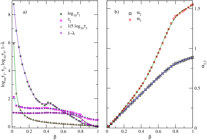
Figure 1: Optimization parameters of modified Havriliak-Negami approximant that is shown in Eq. 3. They, $\alpha_{2}$, $\tau_{1}$, $\tau_{2}$ and $1-\lambda$, follow strictly Eq. 3 while $\tau_{3}$ and $\alpha_{3}$, ($\hat{\alpha}_{3}$ in text), are as in Eq. 4, the latter a simple estimation for the mollifier. $\beta\leq 1$. Solid lines are mathematical adjustments for parameters, which are given in tables 1 and 2.

Therefore we are looking for a function reproducing the main traits of $\psi_{\beta}(\omega)$, namely: $(\frac{\mathrm{d\psi_{\text{$\beta$}}}}{\mathrm{d}\omega})_{\omega=0}\parallel-i$, $\omega^{\beta}*|\psi_{\beta}(\omega)|\stackrel{{\scriptstyle\omega\rightarrow\infty}}{{\longrightarrow}}\mathcal{O}(1)$, and $\psi_{\beta}(\omega)$ $\approx\mathcal{O}(\mathcal{A}p_{2}HN(\omega))$ locally $\forall\omega\in[0,\infty)$ with adiabatic coefficients as parameters in the fit. So with that in mind, and respecting conditions $(\alpha\cdot\gamma)_{1,2}=\beta$ for $\beta<1$, our candidate will take the form:

$$\psi_{\text{$\beta$}}(\omega)\cong\mathcal{AM}_{l,2}HN(\omega)\equiv\frac{\lambda}{(1+i\omega\tau_{1})^{\beta}}+\frac{1-\lambda}{(1+\mathcal{M}_{l}(\omega)(i\omega\tau_{2})^{\alpha_{2}})^{\frac{\beta}{\alpha_{2}}}},$$ (3)

with $\mathcal{M}_{l}(\omega)$, the mollifier of the Havriliak-Negami function, verifying the following boundary conditions

$$\lim_{\omega\rightarrow\infty}\mathcal{M}_{l}(\omega)=1\quad\mathrm{and}\quad\mathcal{M}_{l}(\omega)\approx(\omega\tau_{3})^{\alpha_{3}},\;if\;\omega\approx 0,$$

where $\alpha_{2}+\alpha_{3}$ $\geq 1$.

Undoubtedly to determine the mollifier it is not an easy task and surely its expression as a series could be as difficult of obtaining as the one of $\psi_{\beta}$, and yet the conditions we have imposed on $\mathcal{M}_{l}(\omega)$ may allow an easy estimate of it. So we will put forward as an estimator of mollifier$\mathcal{M}_{l}(\omega)$ the function

$$\hat{\mathcal{M}_{l}}(\omega)\equiv[\frac{2}{\pi}\arctan((\omega\tau_{3})^{\hat{\text{$\alpha$}}_{3}})]^{N},$$ (4)

setting $N=3$ as an appropriate average after a timely optimization for some values of $\beta$.

1.2.2 The squeezed case $\beta>1$

As $\alpha_{1}>1$ and $\alpha_{2}<1$ for $2\geq\beta>1$, when the adjustment to $r_{2}$ sampling is done, it is arguable that a lineal combination of both direction vectors, $(\frac{\mathrm{d}HN_{1,2}(\omega)}{\text{$\mathrm{d}\omega$}}/\omega^{\alpha_{1,2}-1})$, at $\omega=0$ can be parallel to $-i$, since they take values in opposite quadrants (i.e. second and third ones). Nevertheless the magnitude of the derivatives, (zero and infinity respectively), avoids such result, and again the admissible options for $\alpha_{1,2}$ are those of the case $\beta<1$ which as we pointed out contradict the numerical findings. We must proceed again with some modifications of the approximant, however it is not possible now to extend the model of equation 3 to this situation. Firstly the logarithmic second derivatives of $\log_{10}|\psi_{\beta}|$ are qualitatively different for $\beta<1$ and $\beta>1$ cases. (See figures 1 and 2 in [25]). Second only the $\alpha_{2}\cdot\gamma_{2}=\beta$ condition holds while the other becomes $\alpha_{1}\cdot\gamma_{1}\simeq 2\beta$ for the asymptotic behaviour of tails. Besides in the low to medium frequencies range the products $(\alpha\cdot\gamma)_{1,2}$ present a nonlinear trend greater in many cases than the corresponding linear condition of high frequency. (See figure 9 in [25]). In consequence we introduce a peculiar model with two characteristic times in the first Havriliak-Negami relaxation which jointly with the two terms structure of the whole approximant will retain the mentioned characteristics and restrictions for tails, with the sole exception of $\alpha_{0}\cdot\gamma_{1}$ which is to be determined by fitting. The latter in light of the numerical results appears a spurious property or at least a virtual one conceived to explain the sudden change of curvature in a small interval of frequencies, $\nu\lesssim 1$.

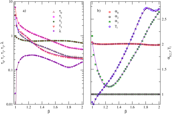
Figure 2: For $\beta\geq 1$ an approximation to $\psi_{\beta}$ is done using the modified approximant $\mathcal{AM}_{g,2}HN$ set in Eq. 5. At left panel parameters: $\text{$\tau$}_{0}$, $\tau_{1}$, $\tau_{2}$, $\tau_{3}$ and $\lambda$. At right panel: $\alpha_{0}$, $\alpha_{2}$, $\alpha_{3}$ and $\gamma_{1}$. Except for $\tau_{3}$ and $\alpha_{3}$, ($\hat{\alpha}_{3}$ in text), all of them are defined in Eq. 5. The former are established in Eq. 6 which describes an estimator of the current mollifier. As in previous graphics the parameters are adjusted with suitable mathematical expressions, (solid lines), given in tables 3 and 4.

Thus when $\beta>1$ the global formula for the approximant it reads:

$$\psi_{\text{$\beta$}}(\omega)\cong\mathcal{AM}_{g,2}HN(\omega)\equiv\frac{\lambda}{(1+i\omega\tau_{1}+(i\omega\tau_{0})^{\alpha_{0}})^{\gamma_{1}}}+\frac{1-\lambda}{(1+\mathcal{M}_{g}(\omega)(i\omega\tau_{2})^{\alpha_{2}})^{\frac{\beta}{\alpha_{2}}}},$$ (5)

with the boundary conditions for the mollifier as

$$\lim_{\omega\rightarrow\infty}\mathcal{M}_{g}(\omega)=1\quad\mathrm{and}\quad\mathcal{M}_{g}(\omega)\sim\mathcal{O}(1),\;if\;\omega\approx 0,$$

where $\alpha_{0}>1$ and $\alpha_{2}\gtrsim 1$.

Again an exact expression for the mollifier is out of scope of present study and we settle for an estimator like

$$\hat{\mathcal{M}}_{g}(\omega)\equiv[\frac{1}{\sqrt[n]{2}}\{1+(\sqrt[n]{2}-1)\frac{2}{\pi}\arctan(\omega\tau_{3})^{\hat{\alpha}_{3}}\}]^{n},$$ (6)

and with an ad hoc choice of $n=3$. With such estimator we will obtain a good approximation to $|\psi_{\beta}|$ which deviates slightly in a neighborhood of $\omega\simeq 2\pi$, (the zone where the maximum of curvature happens in logarithmic scale), although it describes fairly the body of function and quite well the trend and values of tail. (See figure 2 in [25]).

1.2.3 Analysing trends of parameter graphics

Finally in figures 1 and 2 we display the parameters of estimated functions $\hat{\mathcal{AM}_{l,2}HN(\omega)}$ and $\hat{\mathcal{AM}_{g,2}HN(\omega)}$ and their adjustments as functions of $\beta$ (respectively $\beta<1$ and $\beta>1$). In this occasion the interval of frequencies is up to $\nu=10^{12}$, and up to $\nu=10^{6}$ depending upon choice of $\beta$, and the sampling of frequencies is what we called logarithmically homogeneous, i.e. $r_{sl}$. In both cases all the curves have a break, or turnaround, more or less evident according to each one. This occurs for each curve, –within same $\beta$ case–, in the same point ($\beta\approx 0.80$ and $\text{$\beta$}\approx 1.80$). Also during the course of several optimizations such points have changed marginally and the breaks have increased or diminished their sharpness according as we changed the average exponent ($N$, $n$) of equations 4 and 6, data weights or samplings ($r_{2}$, $r_{sl}$). So in conclusion we interpret that such abnormalities are a result of the shape of estimators.

Stretched instance, $\beta<1$

The best option in case $\text{$\beta$}<1$ is to weigh, –while using xmgrace to get a fit [27]–, the tails with option $1/Y^{2}$ to soften the jump and obtain an even adjustment all the way in the interval of frequencies. The value of $N$ also could be lowered but the price to pay is an increasing error for all the matching between both functions, (approximant and $\psi_{\beta}$), around values of $\beta\in(0.1,0.3)$ and $\beta\in(0.7,0.8)$. On the other hand the ability of the new function $\mathcal{AM}_{l,2}HN(\omega)$ for describing the effect that slow variation parameters $\{\alpha,\gamma,\tau\}_{1,2}$ would have in the original Havriliak-Negami functions fully justifies the introduction of mollifier $\mathcal{M}_{l}(\omega)$. Unfortunately the expression of its estimator does not seems good enough in the vicinity of $\omega\approx 0$ since the results do not fulfill the required condition $\alpha_{2}+N\hat{\alpha}_{3}\geq 1$ at all when $\beta\rightarrow 0^{+}$. This is a consequence of having frozen the exponent at $N=3$, we should increase its value till infinity to compensate the empirical trends of $\alpha_{2}$ and $\hat{\alpha}_{3}$ to be zero when $\beta\rightarrow 0^{+}$. However the first term of $\hat{\mathcal{AM}_{l,2}HN(\omega)}$, an almost residual one since $\lambda\approx 0$ for $\beta<0.8$, seems to balance numerically this mathematical unsuitability of the second term of the approximant in the description of $\psi_{\beta}(\omega\approx 0)$. And that is possible since there is no conflict in accounting for a slow diminishing $|\psi_{\beta}|$ in the neighborhood of $\omega\approx 0$, ($\beta<0.10$), using a fast decaying Havriliak-Negami type function, (i.e. of large $\tau$), with the sampling step that we used. For such small values of $\beta$ a neighborhood of zero where $|\psi_{\beta}|\sim 1$ is so elusive that a frequency step of $\delta\nu=10^{-8}$ is too large for considering a description of the modulus gradual decay. (In tables 1 and 2 we wrote the mathematical expressions for the six parameters of $\hat{\mathcal{AM}_{l,2}HN(\omega)}$ as curves depending of variable $\beta$).

Formulae	$\exp\big{[}\{\sum_{s=0}^{4}a_{s}(\beta-1)^{s}\}\exp(-M\beta)\big{]}$	$B+\exp[-M(\beta-1)^{3}]\sum_{s=\text{1}}^{4}b_{s}(\beta-1)^{s}$	$C\beta^{2}\exp[\sum_{s=1}^{7}c_{s}(\beta-1)^{s}]$
$\frac{Parameters}{Constants}$ $M$ $a_{0}$ $a_{1}$ $a_{2}$ $a_{3}$ $a_{4}$ Corr.	$\alpha_{0}\simeq 2$ $\alpha_{2}\simeq 1$ 0.880214 4.1814 1.70465 0.0522961 0.976489 -0.770667 2.74286 2.78766 -2.8097 -2.45835 1.36045 -0.148637 0.963441 0.989417	$\frac{Parameter}{Constants}$ $\hat{\alpha}_{3}$ $M$ 1.45629 $B$ 2.0503 $b_{1}$ -9.16895 $b_{2}$ 30.8241 $b_{3}$ -41.314 $b_{4}$ 22.1584 Corr. 0.998267	$\frac{Parameter}{Constants}$ $\gamma_{1}$ $C$ 0.730891 $c_{1}$ 3.50858 $c_{2}$ -34.1656 $c_{3}$ 153.848 $c_{4}$ -373.845 $c_{5}$ 507.468 $c_{6}$ -359.883 $c_{7}$ 102.995 Corr. 0.999860

Table 3: Optimization parameters of the Eq. 5 approximant, (case $\beta>1$): Formulas and their constants for $\alpha_{0}$, $\alpha_{2}$, $\hat{\alpha}_{3}$ and $\gamma_{1}$.

Squeezed instance, $\beta>1$

Case $\beta>1$ is instead more difficult to adjust in the whole interval of frequencies since no additional weight is possible to use. The kink of $\log_{10}|\psi_{\beta}|$ near $\nu\sim 1$ claims for a body not overlooked which would be the case if tails were given more importance by weighing them as in previous procedure. Besides, the mollifier of Havriliak-Negami function is not enough elaborated and as a consequence appears a bifurcation for each curve of parameters, corresponding the lower branch to the best adjustment to data. Nevertheless if the latter is employed for describing the curves, an abrupt change in trend for them is evident and makes more difficult the handled mathematical expressions in parameter adjustment. We show here only the upper branch of all curves, this leads to a smooth and nice interpolation line for each parameter as seen in tables 3 and 4.

$\exp\big{[}(\frac{1}{\beta})^{p}\sum_{s=0}^{5}d_{s}(\beta-1)^{s}\big{]}$

$\exp\big{[}-M(\beta-1)^{0.1}\big{]}\sum_{s=1}^{4}q_{s}(b-1)^{s}$

$\frac{Parameters}{Constants}$ $\tau_{0}$ $\tau_{1}$ $\tau_{2}$ $\tau_{3}$ $p$ $\equiv 11.5$ $\equiv 11.5$ $\equiv 4.4$ $\equiv 9.8$ $d_{0}$ 1.40526 1.91075 -0.0241828 1.36359 $d_{1}$ -38.3857 -27.9873 -4.7472 -30.3907 $d_{2}$ 503.134 484.97 10.0218 380.42 $d_{3}$ -3368.51 -2810.17 -31.8961 -1955.88 $d_{4}$ 8385.44 7209.62 44.4373 3128.49 $d_{5}$ -9737.49 -7533.20 -28.0215 -2939.76 Corr. 0.999708 0.999695 0.999214 0.999346

$\frac{Parameter}{Constants}$ $\lambda$ $M$ 5.82578 $q_{1}$ 273.583 $q_{2}$ -407.192 $q_{3}$ -3.32942 $q_{4}$ 195.919 Corr. 0.998083

Table 4: Optimization parameters of the Eq. 5 approximant, (case $\beta>1$): Formulas and their constants for $\tau_{0}$, $\tau_{1}$, $\tau_{2}$, $\tau_{3}$ and $\lambda$. See figure 2.

Although we started with a nine parameters ansatz for the approximant $\hat{\mathcal{AM}_{g,2}HN(\omega)}$ is clear from the graphs, (right panel of figure 2), that $\alpha_{0}$ and $\alpha_{2}$ are almost constants. Now the written requirements over them are amply fulfilled. Only there is a small disagree of order $10^{-4}$ from condition $\alpha_{2}(\beta)\simeq 1$ for some values of $\beta$. This is entirely due to competition among parameters and subsequent numerical errors. Meanwhile $\alpha_{0}(\beta)\approx 2$ for all betas, and any of them differ from this number less than 1.5% for $\beta>1$ and only with some significance for beta 1.00 and 1.02, and for $\beta>1.80$. Thus with a slight setting of $\hat{\mathcal{M}}_{g}(\omega)$ has to be possible to write $\mathcal{AM}_{g,2}HN(\omega)$ as a seven parameter function which is more economic computationally. (All the adjustments to this set of parameters are given in tables 3 and 4).

1.3 The role of the ’aide-de-camp’ in the modified approximant

Apart from already explained conditions in the onset of frequencies which makes a Cole-Davidson relaxation suitable to describe the boundary condition of $\frac{d\psi_{\beta}}{d\omega}$, it is obvious that in the interval $\beta\in(0.80,1.00]$ the first term of approximant described in Eq. 3 plays an important role in the approximation since $\lambda$ is not at all negligible. However for the interval $\beta\in[0.02,0.80]$ the story is quite different, almost all its contribution is forced by theoretical considerations as now the share coefficient is really small. To extend this situation and make an adjustment with a one-term approximant in the whole interval $\beta\in(0,1)$, we should prepare a more flexible second term of Havriliak-Negami type in Eq. 3. And with this goal in mind we establish the exponent $N$ of $\hat{\mathcal{M}_{l}}(\omega)$ as a new parameter of the optimization. Namely we shall do the following setting:

$$\psi_{\text{$\beta$}}(\omega)\cong\mathcal{AM}_{l,1}HN(\omega)\equiv\frac{1}{(1+\mathcal{M}_{l}(\omega)(i\omega\tau_{2})^{\alpha_{2}})^{\frac{\beta}{\alpha_{2}}}},$$ (7)

with an estimator to $\mathcal{M}_{l}(\omega)$ similar to that of Eq. 4 though now $N=N(\beta)$ is non constant.

The results, (i.e. the parametric curves of $\beta$), are shown in figure 3, there we note two important features about the behaviour of parameters $\alpha_{2}$ and $\hat{\alpha}_{3}$ and the shape peculiarities of $N(\beta)$. The first characteristic, in the interval $\beta\in(0.80,1.00]$, is that we do not recover the functional form of a Debye relaxation as $\beta\rightarrow 1$. For such a requirement it should happen at least $N\rightarrow 0$ and $\alpha_{2}\rightarrow 1$ as an strong condition, or $\alpha_{2}+N\hat{\alpha}_{3}\simeq 1$ as a weaker one, in that limit. Neither the strong nor weak conditions are fulfilled by the parameters as can be seen in right and left panels of figure 3.

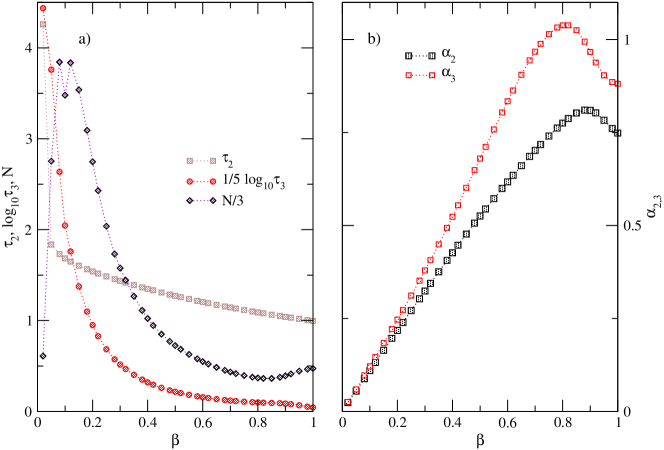
Figure 3: Fitting parameters of Eq. 7 as functions of variable $\beta\leq 1$. Left panel: characteristic times $\text{$\tau$}_{2}$, $\tau_{3}$ and exponent $N(\beta)$, (see Eq. 4). Right panel: frequency exponents $\alpha_{2}$ and $\alpha_{3}$, ($\hat{\alpha}_{3}$ in Eq. 4). The dotted lines are just guides for the eye.

In light of the share coefficient behaviour ($\lambda$) remains an important question: if the auxiliary term dominated by it in the modified approximant is really necessary. (See left panel in figure 1). Or if instead it is only needed to ’unfreeze’ the exponent $N$ in the estimator $\hat{\mathcal{M}_{l}}(\omega)$ of the mollifier, (see Eq. 4), to adjust $\psi_{\beta}(\omega)$ properly with only one term: the mollified Havriliak-Negami function.

The second flaw is patent when we realize that it is not possible, in the interval $\beta\in(0.02,0.10)$, to hold the condition $\alpha_{2}+N\hat{\alpha}_{3}\geq 1$ when $\alpha_{2}\rightarrow 0^{+}$ and $\hat{\alpha}_{3}\rightarrow 0^{+}$ since $N$ is finite and decreasing as $\beta\rightarrow 0$. These trends of alpha parameters are attested, jointly with the $N$ one, and depicted in figure 3 again. In conclusion the modified relaxation of Havriliak-Negami fails in the adjustment at both ends of $\beta$ interval and it is not hard to imagine the difficulties it has to describe an environment of $|\psi_{\beta}|\sim 1$, (i.e. $\omega\approx 0$), with a poor sampling of very low frequencies, (as is the case of ours for so small values of beta). The tails obviously, in such a situation, lead the adjustment and the mentioned requirements about the behaviour of $\frac{d\psi_{\beta}}{d\omega}$ near $\omega\approx 0$ should be imposed externally. At this event the best option to save both flaws is to maintain the optimization with a two-terms approximant like that of Eq. 3.

At last a further reason to keep the expression of Eq. 3 is to have a formal similarity with Eq. 5 for the case $\beta>1$ which makes more manageable the treatment and analysis of the problem in the whole interval $\beta\in(0,2)$.

2 Comparison and discussion: Suitability of formulae

In light of these circumstances we will consider the frequency-averaged relative error, (among data $\psi_{\beta}(\omega)$ and test functions), as an indicator of reconstruction capability for any of the proposed Havriliak-Negami approximants. As it has been patent till now most of the present discussion here refers to the suitability of pairs proposed to describe the modulus of data $|\psi_{\beta}|$. We must be aware that aside from the results here discussed some additional tuning of phase should be sought. Different one with each model for approximation we use. Even so, without all the benefits of the phase, an accurate adjustment between data and approximants makes this methodology of multiple Havriliak-Negami summands useful to determine form parameters in dielectric spectroscopy experiments, or in systematic search of them by means of genetics algorithms.

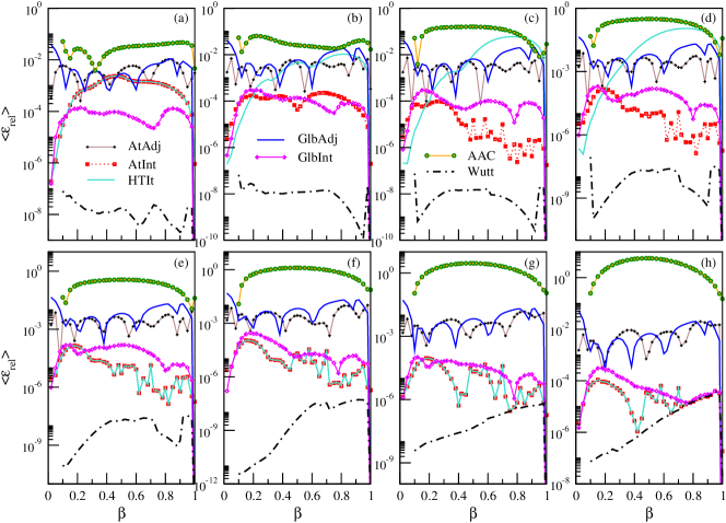
Figure 4: Frequency-averaged relative error, $\langle\varepsilon_{rel}(\psi_{\beta}^{(a)},\psi_{\beta}^{(b)},\omega_{m},\omega_{x})\rangle$, for data $\psi_{\beta}\equiv\psi_{\beta}^{(a)}$ obtained with Mathematica^TM and function values $\psi_{\beta}^{(b)}$ of models AAC (circle), Wutt (dot-dashed), AtAdj (plusses), AtInt (squares), HTIt (light solid), GlbAdj (dark solid) and GlbInt (diamonds). Eight frequency windows, whose details are written in the text, and two types of samplings –linear from (a) to (d) and logarithmic from (e) to (h)– are shown for interval $0<\beta\leq 1$.

Previously, a frequency-averaged relative error for the moduli of functions was defined as:

$$\langle\varepsilon_{rel}(\psi_{\beta}^{(a)},\psi_{\beta}^{(b)},\omega_{m},\omega_{x})\rangle=\frac{\int_{\omega_{m}}^{\omega_{x}}|1-\frac{|\psi_{\beta}^{(b)}|}{|\psi_{\beta}^{(a)}|}|\mathrm{d}\omega}{\omega_{x}-\omega_{m}}.$$

Such error function is depicted in graphics 4 and 5. There it was calculated for the different models described in a previous paper, [25], and in the present one, and also for other two models found in literature (see references [19, 20]). In particular, the errors for a Havriliak-Negami function, the three models described above (double H-N, atlas of aproximants and modified H-N), two variants of the last ones with parameters calculated via formulae given in tables 1 to 4 in [25], and the numerical solution obtained from the C code in reference [19] are given, when $\beta\leq 1$, in figure 4. Same models with $\beta>1$, except 1HN of AAC (Ref. [20]), are portrayed in figure 5.

The frequency windows studied are: (a) $[\omega_{m},\omega_{x})/2\pi$ $=[0,1)$, (b) $[1,10)$, (c) $[10,100)$, (d) $[100,500]$ in the upper row of both figures. They followed a linear sampling with $\delta\nu$ $=\frac{1}{999.999}$, conversely the lower rows were logarithmic, homogeneous in each decade in the way we already explained. Their intervals of frequencies are: (e) $[100,10^{3})$, (f) $[10^{3},10^{6})$, for both graphs, but (g) $[10^{6},10^{9})$, (h) $[10^{9},10^{12}]$ with $\beta\leq 1$, and (g’) $[10^{6},10^{7}]$ when $\beta>1$.

For a quick sight inside the plots in 4 and 5 we have tagged the models already explained. We remind that $\psi_{\beta}^{(a)}(\omega)\equiv\psi_{\beta}(\omega)$ was obtained from the direct calculation of Fourier integral and is the same reference for all errors $\langle\varepsilon_{rel}\rangle$ calculated with different test models $\psi_{\text{$\beta$}}^{(b)}$ which are now listed as: AAC, the Havriliak-Negami approximation cited in ref. [20]. Wutt, the C library of reference [19] which employs the power series for low and high frequencies and an effective numerical method for the intermediary frequencies in the interval $\beta\in$ $[0.1,2.0]$. AtAdj is the label assigned to the model of equation 2, and the same is true for the symbol AtInt. The distinction is that while the parameters $\{\alpha_{1,2},\gamma_{1,2},\tau_{1,2},\lambda\}$ in the first case are calculated following the formulas in tables 1 to 8 of [25], in the last one are obtained from the points directly obtained of error minimization and depicted in graphics 5, 6, 7 and 8 of [25]. For the sake of clarity we have repeated the latter results showing separately each part which follows the eq. 1 for low or high frequencies (head and tail functions of equation 2). It allows to appreciate where in the frequency interval the individual approximant diverges from the data, and which one is exactly its contribution to the atlas of approximants. The transition from a plain downhill to a potential tail ($\nu^{-\beta}$) it is then quite clear. This is called HTIt. Besides all the three previous models refer to the range $[0.02,2.00]$ of shape parameter $\beta$.

The last assertion it is also true for labels GlbAdj and GlbInt though two different formulas and their respective implementations are employed, the equations 3 and 4 for $\beta\leq 1$ and the equations 5 and 6 for $\beta>1$. Again the first tag refers to the adjusted parameters (see tables 1, 2, 3 and 4) and the second to the original points as depicted in figures 1 and 2.

2.1 Models response in the stretched case

In figure 4, AAC, the approximation with only one HN function, shows the biggest of all errors for the models here presented and the interval $0<\beta\leq 1$. The best result is of course that of Wutt which combine analytics and numerics. Meanwhile the atlas described by equation 2, (i.e. AtInt), works quite well even in the interval of very low frequencies where we demonstrated that one of the functions of the approximant should be a Cole-Davidson relaxation or a modified version of it, –this depends on if $\beta$ is less than or greater than unit. (See Eqs. 3 and 5). Besides, it holds good terms in the medium range thanks to the change of describer function, (i.e. from head, $\mathcal{A}p_{2,l}HN$, to tail, $\mathcal{A}p_{2,h}HN$; see figure 4 panel (b)). The performance of this swap is even better for high frequencies because the matching with data exceeds expectations and the approximation has not required any restriction in the product $(\alpha\cdot\gamma)_{1,2}$. This reinforces our previous conclusion [24], and points to the true nature of $\psi_{\beta}$ as a sum of a Havriliak-Negami pair with almost constant coefficients which only change significatively as $1>\omega\rightarrow 0$ [28]. Such important transition is highlighted in figures 4 and 5 by the discrepancy between model AtInt (squares) and HTIt (light solid line) and reminds us the need for at least two charts (one for $\nu<1$ the other for $\nu>1$) in the description of the whole function $\psi_{\beta}$. Usually this approach is not taken in consideration in the literature since only one set of parameters $\{\alpha,\gamma,\tau,\lambda\}$ is employed to match the data, or if considered is misinterpreted due to the usage of a time scale factor in the stretched exponential (i.e. $\exp-(t/\tau_{KWW})^{\beta}$) [29]. See panels (a) to (d) in figure 4.

It is worth to note how the Havriliak-Negami approach AAC starts to work better than the double approximant HTIt in the range of medium-to-high frequencies, according as $0.8<\beta\rightarrow 1$. It sounds logical since $\text{$\beta$}\rightarrow 1$ implies $\lambda\rightarrow 0$, and this final value is a pathology for the double sum of HN functions quite difficult to treat numerically. Such problem is not evident using the atlas AtInt since the approximant of tail $\mathcal{A}p_{2,h}HN$ takes the control over $\mathcal{A}p_{2,l}HN$ in such frequency interval. The former function besides, at very high $\nu$’s and with $\beta$ near $1.00$, shows similar errors to the results of numerical-analytic method Wutt. Now the major problem for both of them will be the numerical oscillations of reference data. See panels (g) and (h) in figure 4.

The differences of error between model AtAdj and AtInt present clearly two regions. One in the low frequencies zone ($\nu<1$) the other in the high frequency one ($\nu>1$), as it is usual coinciding with the onset of potential behaviour for tails. In the first case it is the lack of ability of the double approximant with constant parameters to approach data, what gets closer both models. This is shown in figure 4a and is more conspicuous when $\beta\sim 0.40$. In the second case where both models split apart more than one order of magnitude the reason for this is more subtle because the correspondence between $\psi_{\beta}^{(a)}$ and $\psi_{\beta}^{(b)}$ is tighter as both functions follow a quite similar potential decaying. (See graph 4, panels (b) to (h), and figure 9 in [25]). What makes such difference between AtInt and AtAdj is an extra error provided for each of the parameters $\alpha_{1,2}$, $\gamma_{1,2}$, $\tau_{1,2}$ and $\lambda$. An additional contribution which is consequence of the fitting of parametric curves to optimized points. Then it would be desirable to reduce those inputs binding the parameters to relationships as the already mentioned $(\alpha\cdot\gamma)_{1,2}\sim\beta$. Nevertheless, we feel that some further work should be done to link the conduct of $\tau(\text{$\beta$})_{1,2}^{\beta}$ and $\lambda$ to the coefficients of the analytical series for $\psi_{\beta}$, and so in the absence of them we have presented the models drawn from eq. 2 free of any external constraints.

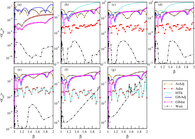
Figure 5: Relative error, $\langle\varepsilon_{rel}(\psi_{\beta}^{(a)},\psi_{\beta}^{(b)},\omega_{m},\omega_{x})\rangle$, for data $\psi_{\beta}\equiv\psi_{\beta}^{(a)}$ obtained with Mathematica^TM and test values $\psi_{\beta}^{(b)}$ of models: Wutt (dot-dashed), AtAdj (plusses), AtInt (squares), HTIt (light solid), GlbAdj (dark solid) and GlbInt (diamonds). Seven frequency windows and two types of samplings –linear from (a) to (d) and logarithmic from (e) to (g)– are shown. Maximum frequency in panel (g) is reduced to $\nu_{x}=10^{7}$ due to glitches and numerical noise of data beyond this point. $1<\beta\leq 2$.

As a novelty we introduced here two global models to simulate the data, namely GblInt (optimized points) and GblAdj (adjusted parameters). Watching them carefully in the various intervals of frequency one can realize how the performances are similar to the models of Havriliak-Negami double approximants, AtInt and AtAdj, respectively. Also is possible to observe how for the low frequency range, $\nu<1$, the model GblInt outperforms to AtInt, although this one later improves and is usually better for the high frequencies in accuracy. (See in panels (a) to (h) of figure 4 the square and diamond curves). Also for the global model, the aggregated error of several independent parameters spoils the result making alike the error curves of cases AtAdj and GblAdj, (plusses and dark solid lines in graphics). Therefore the drastic displacement of relative error lines towards a lesser precision for models with adjusted parameters $\{\alpha_{1,2},\gamma_{1,2},\tau_{1,2},\lambda\}(\beta)$ points to the need for strict relationships among them and good descriptions of functional dependence with the shape parameter $\beta$.

However it is important to emphasize how proposed estimators of mollifiers, ($\hat{\mathcal{M}}_{l,g}$ in Eqs. 4 and 6), are subject to many “ad hoc” restrictions, mainly deduced of data traits and information obtained from the behavioral changes of $\alpha_{1,2},\gamma_{1,2},\tau_{1,2},\lambda$ curves while changing the regime of frequencies from low to high. The most significative restraint here is the fact the $\hat{\mathcal{M}}_{l,g}$ functions are set as real ones when they should value in the complex field. As we have seen before, in Eqs. 3 and 5, near $\omega\approx 0^{+}$ the dominant demeanor of $\hat{\mathcal{M}}_{l,g}(\omega)$ is determined without consider further modifications to the phase $i^{\alpha_{2}}$ since the frequency factor $\omega^{\alpha_{2}+*}$ extinguishes such contribution quickly and only remains the one of extended Cole-Davidson term. Nevertheless the role the phase plays is over the entire interval of frequencies and, although to our present purpose of describing the modulus accurately it is not crucial this bias in the argument of the approximation $\mathcal{AM}_{l,g,2}HN$, it is important to point out the need of a mollifier in complex series for proper description of $\psi_{\beta}$.

It seems promising, from an analytical point of view, that a strategy to sum up a quite difficult series in the neighborhood of $\omega\approx 0^{+}$ comes from the help of an extended Havriliak-Negami pair. Perhaps could be interesting to decide the mollifier’s functional form with the aid of series, integrals or equations which determine $\psi_{\beta}$. Mainly when $\omega\rightarrow 0$, for $\beta<1$, or when $\omega\rightarrow\infty$ for $\beta>1$, the most difficult cases for power series involved [8, 16, 29].

Obviously, in the light of the problems we face when using unsuitable functions as estimators of $\mathcal{M}_{l,g}(\omega)$, it is suggested that a similar ’loss’ of phase could happen in the atlas approximation of eq. 2 to data. And consequently foresee a mild shift in the argument of whole function $\mathcal{A}p_{2}HN(\omega)$ at high frequencies. This displacement is due to the way the tail functions $\mathcal{A}p_{2,h}HN(\omega)$ are determined. Data are pruned in a logarithmic pace and the important information at low frequencies, –the plateau–, is removed when optimizing tail parameters, something is not made in the case of head functions, $\mathcal{A}p_{2,l}HN(\omega)$. All this does not impact very much on the approach to the modulus, as we saw in graphics of figures 4 and 5, but suggests a share parameter fully complex, i.e. $\lambda\in\mathbb{C}-\mathbb{R}$. Unfortunately it would add a new degree of freedom and would overshadow the discussion about modulus characteristics in absence of a thorough treatment of the data phase.

Apart its mentioned inability to describe the very low frequency range, the double Havriliak-Negami approximant, $\mathcal{A}p_{2}HN_{\alpha,\gamma,\tau,\lambda}(\omega)$, will not present such difficulties while describing the argument, –much less the modulus–, of data $\psi_{\beta}$.

2.2 Models response in the squeezed case

The last stay in this discussion is the figure 5 that shows relative errors of the six previous models for shape parameter interval $1<\beta\leq 2$. As predicted by first and second logarithmic derivative, (see frames a) and b) of fig. 2 in [25]), there is a sudden change of behaviour in the slope of $|\psi_{\beta}|$ from flatness to a potential decline $\omega^{-\beta}$ in a relatively small interval of frequencies. (See frame c) of same graphics in [25]). This is a much more sharper and distinct transition than in case $\beta\leq 1$, which forces the existence of a different set of constraints for products $\alpha\cdot\gamma$ in the double Hav.-Neg. approximation, as clearly shows figure 9 in [25]. All this oblige to abandon quickly the HTIt model, (light solid line in 5, panels (a) to (d)), in favor of AtInt because the latter holds itself quite close to the potential tail and shares same description of $|\psi_{\beta}|$ with the former at very low frequencies. (See squares inside panels (a), and (b) to (g) in figure 5).

Again, as with $\beta\leq 1$, a big distance in terms of relative error separates AtInt and AtAdj, and as before this gap is attributed to a collective error subscribed by each individual parameter, whenever every uncertainty is caused by obtaining the appropriate parameter from a pertinent fitting function along all values of $\beta$. However for the models GlbInt and GlbAdj such distance doesn’t exist at medium frequencies and thereafter, i.e. $\nu>1$. (See diamonds and dark solid line in graphics of figure 5). It seems that model GlbInt it is not able to keep track of data tail so close as AtInt does. Surely the ’bi-chronicity’ or the mollifier in functional form of Eq. 5 should be revisited to give a proper account of directional twist of data near $\nu\sim 1$, and thus to diminish the error below the collective contribution of parameters. As in fact it happens at low frequencies, (see figure 5a). Nevertheless, as far we know, this is one of the few attempts to describe globally the Fourier transform $\psi_{\beta}$ for $\beta>1$ with an analytical model albeit approximate, so each piece of formula $\mathcal{AM}_{g,2}HN(\omega)$ has great value for future mathematical inquiries.

Finally we should point out how, at very large frequencies, the potential description overcomes some numerical difficulties experienced by Wutt model for large $\beta$ values, i.e. $\beta\geq 1.60$. (See figures 5f and 5g).

3 Conclusions

The present work is devoted to a compact description of the Fourier Transform of the Kohlrausch relaxation. As any reconstruction of this function as from spectral data should heavily depend on the information of frequencies near zero since tails will be surely corrupted by noise, an extra effort has to be made to manufacture a global function mimicking all aspects of this transform from low to high frequencies. Thus, two new sets of such models are proposed, and a detailed discussion on their errors compared to numerical control calculations generated directly by evaluating the Fourier integrals is made.

We found how the approximation with a double H-N function always underestimates $\psi_{\beta}$ in the low frequency range, ($\nu<0.1$). And although it is a small difference forces us to change those values of parameters $\{(\alpha,\gamma,\tau)_{1,2},\lambda\}$ already obtained in the range of medium frequencies.

This repeats again in the transition from medium to high, or very high, frequencies. Nevertheless the double Havriliak-Negami approximation is close enough to the original function as to describe it along a wide range of frequencies before the variation can be noticed. Moreover the parameters should not be regarded as varying, if the interval where the approximation is performed only comprises very high frequencies.

Thus, due to the slow variation of parameters of the approximant with the frequency, (adiabatic parameters), instead of a global function with $\omega-$dependent $\{(\alpha,\gamma,\tau)_{1,2},\lambda\}$, we employed different charts of double Havriliak-Negami sums to describe locally $\psi_{\beta}(\omega)$. We found that using two charts is a good approximation, enough to establish an atlas, however the differences at low frequencies still persist with such number of maps. The inclusion of a third one in the neighborhood of zero, i.e. $\nu\approx 0$, should be convenient, though the existence of an exact analytical series of powers in terms of Cole-Cole relaxations [4, 28], (i.e. $1/(1+(i\omega)^{\beta})$), for $\psi_{\beta}$ suggests the radius of such chart will depend on $\beta$ [29]. What it makes difficult and cumbersome working with an atlas of three maps.

The question whether it is possible to sum up the series of Cole-Cole terms at $\nu=0$, or it is possible to write the atlas of Havriliak-Negami charts just in a global way, seems to have a positive answer. We presented two ansätze for extending the double Havriliak-Negami approximation, – that has proved to be successful locally –, which describe along several decades in frequency, and with enough functional proximity, the data of $|\psi_{\beta}|$. By means of rough estimates of the mollifiers of these new testing relaxations, we have found a good agreement with data moduli signaling a path for a future close approximation in the complex domain to the series, or numerical integrals, of the Fourier Transform $\psi_{\beta}$.

References

- [1] P. Debye, Ver. Deut. Phys. Gesell. 15, 777 (1913).
- [2] S. Havriliak and S. Negami, J. Polym. Sci. Part C 14, 99 (1966).
- [3] S. Havriliak and S. Negami, Polymer 8, 161 (1967).
- [4] K. S. Cole and R. H. Cole, J. Phys. Chem. 9, 341 (1941).
- [5] D. W. Davidson and R. H. Cole, J. Chem. Phys. 19, 1484 (1951).
- [6] R. Kahlau, D. Kruk, Th. Blochowicz, V. N. Novikov, and E. A. Rössler, J. Phys.: Codens. Matter 22, 365101 (2010).
- [7] A. Stanislavsky, K. Weron and J. Trzmiel, Eur. Phys. Lett. 91, 40003 (2010).
- [8] A. Wintner, Duke Math. J. 8, 678 (1941).
- [9] P. Humbert, Bull. Sci. Math. 69, 121 (1945).
- [10] H. Pollard, Bull. Am. Math. Soc. 52, 908 (1946).
- [11] G. Williams and D. C. Watts, Trans. Faraday Soc. 66, 80 (1970).
- [12] G. Williams, D. C. Watts, S. B. Dev, and A. M. North, Trans. Faraday Soc. 67, 1323 (1971).
- [13] C. P. Lindsey and G. D. Patterson, J. Chem. Phys. 73, 3348 (1980).
- [14] R. Hilfer, Phys. Rev. E 65, 061510 (2002).
- [15] E. Capelas de Oliveira, F. Mainardi, and J. Vaz Jr., Eur. Phys. J. Special Topics 193, 161 (2011).
- [16] M. Dishon, G.H. Weiss, and J.T. Bendler, J. Res. Natl. Bur. Stand. 90, 27 (1985).
- [17] H. Schaefer, E. Sternin, R. Stannarius, M. Arndt, and F. Kremer, Phys. Rev. L. 76, 2177 (1996).
- [18] Ch. R. Snyder and F. I. Mopsik, Phys. Rev. B 60, 984 (1999).
- [19] J. Wuttke, preprint: arXiv:0911.4796v1, (2009); Algorithms 5, 604 (2012).
- [20] F. Alvarez, A. Alegria, and J. Colmenero, Phys. Rev. B 44, 7306 (1991).
- [21] F. Alvarez, A. Alegria, and J. Colmenero, Phys. Rev. B 47, 125 (1993).
- [22] W. Weibull, J. Appl. Mech. Trans. ASME. 18, 293 (1951).
- [23] J. R. Macdonald and R. L. Hurt, J. Chem. Phys. 84, 496 (1986).
- [24] J.S. Medina, R. Prosmiti, P. Villareal, G. Delgado-Barrio, and J. V. Alemán, Phys. Rev. E 84, 066703 (2011).
- [25] J.S. Medina, R. Prosmiti, and J. V. Alemán, preprint: arXiv:1509.07893, (2015).
- [26] F. W. Warner, Foundations of Differentiable Manifolds and Lie Groups, Scott, Foresman and Co. (1971); Springer, ISBN: 978-0-387-90894-6 (1983).
- [27] P. Turner, E. Stambulchik, and Grace Development Team, http://plasma-gate.weizmann.ac.il/Grace
- [28] G. H. Weiss, M. Dishon, A. M. Long, J. T. Bendler, A. A. Jones, P. T. Inglefield, and A. Bandis, Polymer 35, 1880 (1994).
- [29] Ch. Schroeder and O. Steinhauser, J. Chem. Phys. 132, 244109 (2010).