all
2 \acmNumber3 \acmArticle1 \articleSeq1 \acmYear2016 \acmMonth1
Efficient Redundancy Techniques
for Latency Reduction in Cloud Systems
Abstract
In cloud computing systems, assigning a task to multiple servers and waiting for the earliest copy to finish is an effective method to combat the variability in response time of individual servers, and reduce latency. But adding redundancy may result in higher cost of computing resources, as well as an increase in queueing delay due to higher traffic load. This work helps understand when and how redundancy gives a cost-efficient reduction in latency. For a general task service time distribution, we compare different redundancy strategies in terms of the number of redundant tasks, and time when they are issued and canceled. We get the insight that the log-concavity of the task service time creates a dichotomy of when adding redundancy helps. If the service time distribution is log-convex (i.e. log of the tail probability is convex) then adding maximum redundancy reduces both latency and cost. And if it is log-concave (i.e. log of the tail probability is concave), then less redundancy, and early cancellation of redundant tasks is more effective. Using these insights, we design a general redundancy strategy that achieves a good latency-cost trade-off for an arbitrary service time distribution. This work also generalizes and extends some results in the analysis of fork-join queues.
This work was supported in part by NSF under Grant No. CCF-1319828, AFOSR under Grant No. FA9550-11-1-0183, and a Schlumberger Faculty for the Future Fellowship. This work was presented in part at the Allerton Conference on Communication, Control and Computing 2015, and ACM Sigmetrics Mathematical Modeling and Analysis Workshop 2015. Authors’ email addresses: Gauri Joshi: gaurij@andrew.cmu.edu (this author was at MIT at the time of this work); Emina Soljanin: emina.soljanin@rutgers.edu; Gregory W. Wornell: gww@mit.edu
1 INTRODUCTION
1.1 Motivation
An increasing number of applications are now hosted on the cloud. Some examples are streaming (NetFlix, YouTube), storage (Dropbox, Google Drive) and computing (Amazon EC2, Microsoft Azure) services. A major advantage of cloud computing and storage is that the large-scale sharing of resources provides scalability and flexibility. However, an adverse effect of the sharing of resources is the variability in the latency experienced by the user due to queueing, virtualization, server outages etc. The problem becomes further aggravated when the computing job has several parallel tasks, because the slowest task becomes the bottleneck in job completion. Thus, ensuring fast and seamless service is a challenging problem in cloud systems.
One method to reduce latency that has gained significant attention in recent years is the use of redundancy. In cloud computing, replicating a task on multiple machines and waiting for the earliest copy to finish can significantly reduce the latency [Dean and Barroso (2013)]. Similarly, in cloud storage systems, requests to access a content can be assigned to multiple replicas, such that it is only sufficient to download one replica. However, redundancy can result in increased use of resources such as computing time, and network bandwidth. In frameworks such as Amazon EC2 and Microsoft Azure which offer computing as a service, the computing time spent on a job is proportional to the cost of renting the machines.
| (Replicated) Case | General | |
|---|---|---|
| Full forking to all servers | \pbox[c]4.6cm Section 5 | |
| Comparison of strategies with and without early task cancellation | \pbox[c]4.6cmSection 7 | |
| Bounds on latency and cost, and the diversity-parallelism trade-off | ||
| Partial forking to out of servers | \pbox[c]4.6cm Section 6 | |
| Effect of and the choice of servers on latency and cost | \pbox[c]4.6cmSection 8 | |
| General redundancy strategy for cost-efficient latency reduction |
1.2 Organization of this Work
In this work we aim to understand the trade-off between latency and computing cost, and propose efficient strategies to add redundancy. We focus on a redundancy model called the fork-join model, where a job is forked into tasks such that completion of any tasks is sufficient to finish the job. In Section 2 we formally define this model and its variants. Section 3 summarizes related previous work and our contributions. Section 4 gives the key preliminary concepts used in this work.
The rest of the paper studies different variants of the fork-join model in increasing order of generality, as shown in Table 1.1. In Section 5 and Section 6 we focus on the (replicated) case. Section 5 considers full replication of a job at all servers, and compares different strategies of canceling redundant tasks. In Section 6 we consider partial replication at out of servers.
In Section 7 and Section 8, we move to the general case, which requires a significantly different style of analysis than the case. In Section 7 we consider full forking to all servers, and determine bounds on latency and cost, generalizing some of the fundamental work on fork-join queues. For partial forking, we propose a general redundancy strategy in Section 8. System designers looking for a practical redundancy strategy rather than theoretical analysis may skip ahead to Section 8 after the problem setup in Section 2.
Finally, Section 9 summarizes the results and provides future perspectives. Properties and examples of log-concavity are given in Appendix A. Proofs of the and general cases are deferred to Appendix B and Appendix C respectively.
2 SYSTEM MODEL
2.1 Fork-Join Model and its Variants
Definition 1 ( fork-join system)
Consider a distributed system with statistically identical servers. Jobs arrive to the system at rate , according to a Poisson process111The Poisson assumption is required only for the exact analysis and bounds on latency (equations (5), (7), (8), (11), (16), (17), and (24)). All other results on , and comparison of replication strategies in heavy traffic hold for any arrival process.. Each job is forked into tasks that join first-come first-served queues at each of the servers. The job is said to be complete when any tasks are served. At this instant, all remaining tasks are canceled and abandon their respective queues immediately.
After a task of the job reaches the head of its queue, the time taken to serve it can be random due to various factors such as disk seek time and sharing of computing resources between multiple processes. We model this service time by a random variable , with cumulative distribution function (CDF) . The tail distribution (inverse CDF) of is denoted by . We use to denote the smallest of i.i.d. random variables .
We assume that the service time is i.i.d. across tasks and servers. Thus, if a task is replicated at two different servers, the service times of the replicas are independent and identically distributed. Dependence of service time on the task itself can be modeled by adding a constant to . More generally, may be a random variable. Although we do not consider this case here, the results in this paper (particularly Section 5) can be extended to consider correlated service times.
Fig. 2 illustrates the fork-join system. The job exits the system when any out of tasks are complete. The case corresponds to a replicated system where a job is sent to all servers and we wait for one of the replicas to be served. The fork-join system with can serve as a useful model to study content access latency from an erasure coded distributed storage system. Approximate computing applications that require only a fraction of tasks of a job to be complete can also be modeled using the fork-join system.
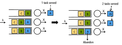
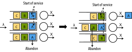
We consider the following two variants of this system, which could save the amount of redundant time spent by the servers of each job.
-
1.
fork-early-cancel system: Instead of waiting for tasks to finish, the redundant tasks are canceled when any tasks reach the heads of their queues and start service. If more than tasks start service simultaneously, we retain any chosen uniformly at random. Fig. 2 illustrates the fork-early-cancel system. In Section 5 we compare the systems with and without early cancellation.
-
2.
partial fork-join system: Each incoming job is forked into out of the servers. When any tasks finish service, the redundant tasks are canceled immediately and the job exits the system. The servers can be chosen according to different scheduling policies such as random, round-robin, least-work-left (see [Harchol-Balter (2013), Chapter 24] for definitions) etc. In Section 6 we develop insights into the best choice of , and the scheduling policy.
Other variants of the fork-join system include a combination of partial forking and early cancellation, or delaying invocation of some of the redundant tasks. Although not studied in detail here, our analysis techniques can be extended to these variants. In Section 8 we propose a general redundancy strategy that is a combination of partial forking and early cancellation.
2.2 Latency and Cost Metrics
We now define the metrics of the latency and resource cost whose trade-off is analyzed in the rest of the paper.
Definition 2 (Latency)
The latency is defined as the time from the arrival of a job until it is served. In other words, it is the response time experienced by the job.
In this paper we focus on analyzing the expected latency . Although is a good indicator of the average behavior, system designers are often interested in the tail of the latency. For many queueing problems, determining the distribution of response time requires the assumption of exponential service time. In order to consider arbitrary, non-exponential service time distribution , we settle for analyzing here.
Definition 3 (Computing Cost)
The computing cost is the total time spent by the servers serving a job, not including the time spent in the queue.
In computing-as-a-service frameworks, the computing cost is proportional to money spent on renting machines to run a job on the cloud222Although we focus on this cost metric, we note that redundancy also results in a network cost of making Remote-Procedure Calls (RPCs) made to assign tasks of a job, and cancel redundant tasks. It is proportional to the number of servers each job is forked to, which is for the fork-join model described above. In the context of distributed storage, redundancy also results in increased use of storage space, proportional to . The trade-off between delay and storage is studied in [Joshi et al. (2012), Joshi et al. (2014)]..
3 PREVIOUS WORK AND MAIN CONTRIBUTIONS
3.1 Related Previous Work
Systems Work: The use of redundancy to reduce latency is not new. One of the earliest instances is the use of multiple routing paths [Maxemchuk (1975)] to send packets in networks; see [Kabatiansky et al. (2005), Chapter 7] for a detailed survey of other related work. A similar idea has been studied [Vulimiri et al. (2013)] in the context of DNS queries. In large-scale cloud computing frameworks, several recent works in systems [Dean and Ghemawat (2008), Ananthanarayanan et al. (2013), Ousterhout et al. (2013)] explore straggler mitigation techniques where redundant replicas of straggling tasks are launched to reduce latency. Although the use of redundancy has been explored in systems literature, there is little work on the rigorous analysis of how it affects latency, and in particular the cost of resources. Next we review some of that work.
Exponential Service Time: The fork-join system was first proposed in [Joshi et al. (2012), Joshi et al. (2014)] to analyze content download latency from erasure coded distributed storage. These works consider that a content file coded into chunks can be recovered by accessing any out of the chunks, where the service time of each chunk is exponential. Even with the exponential assumption analyzing the fork-join system is a hard problem. It is a generalization of the fork-join system, which was actively studied in queueing literature [Flatto and Hahn (1984), Nelson and Tantawi (1988), Varki et al. (2008)] around two decades ago.
Recently, an analysis of latency with heterogeneous job classes for the replicated () case with distributed queues is presented in [Gardner et al. (2015)]. Other related works include [Shah et al. (2014), Kumar et al. (2014), Xiang et al. (2014), Kadhe et al. (2015)]. A common thread in all these works is that they also assume exponential service time.
General Service Time: Few practical systems have exponentially distributed service time. For example, studies of download time traces from Amazon S3 [Liang and Kozat (2014), Chen et al. (2014)] indicate that the service time is not exponential in practice, but instead a shifted exponential. For service time distributions that are ‘new-worse-than-used’ [Cao and Wang (1991)], it is shown in [Koole and Righter (2008)] that it is optimal to replicate a job at all servers in the system. The choice of scheduling policy for new-worse-than-used (NWU) and new-better-than-used (NBU) distributions is studied in [Kim et al. (2009), Shah et al. (2013), Sun et al. (2015)]. The NBU and NWU notions are closely related to the log-concavity of service time studied in this work.
The Cost of Redundancy: If we assume exponential service time then redundancy does not cause any increase in cost of server time. But since this is not true in practice, it is important to determine the cost of using redundancy. Simulation results with non-zero fixed cost of removal of redundant requests are presented in [Shah et al. (2013)]. The expected computing cost spent per job was previously considered in [Wang et al. (2014), Wang et al. (2015)] for a distributed system without considering queueing of requests. In [Joshi et al. (2015)] we presented an analysis of the latency and cost of the fork-join with and without early cancellation of redundant tasks.
| Log-concave service time | Log-convex service time | |||
|---|---|---|---|---|
| Latency-optimal | Cost-optimal | Latency-optimal | Cost-optimal | |
| Cancel redundancy early or keep it? | \pbox[c]3.75cmLow load: Keep Redundancy, | |||
| High load: Cancel early | Cancel early | Keep Redundancy | Keep Redundancy | |
| Partial forking to out of servers | \pbox[c]3.7cmLow load: (fork to all), | |||
| High load: (fork to one) | (fork to all) | (fork to all) | ||
3.2 Main Contributions
The main differences between this and previous works are: 1) we consider a general service time distribution, instead of exponential service time and, 2) we analyze the impact of redundancy on the latency, as well as the computing cost (total server time spent per job). Incidentally, our computing cost metric also serves as a powerful tool to compare different redundancy strategies under high load.
The latency-cost analysis of the fork-join system and its variants gives us the insight that the log-concavity (and respectively, the log-convexity) of , the tail distribution of service time, is a key factor in choosing the redundancy strategy. Here are some examples, which are also summarized in Table 3.1.
-
•
By comparing the systems (fork to , wait for any ) with and without early cancellation, we can show that early cancellation of redundancy can reduce both latency and cost for log-concave , but it is not effective for log-convex .
-
•
For the partial-fork-join system (fork to out of , wait for any ), we can show that forking to more servers (larger ) is both latency and cost optimal for log-convex . But for log-concave , larger reduces latency only in the low traffic regime, and always increases the computing cost.
Using these insights we also develop a general redundancy strategy to decide how many servers to fork to, and when to cancel the redundant tasks, for an arbitrary service time that may be neither log-concave nor log-convex.
4 PRELIMINARY CONCEPTS
We now present some preliminary concepts that are vital to understanding the results presented in the rest of the paper.
4.1 Using to Compare Systems
Since the cost metric is the expected time spent by servers on each job, higher implies higher expected waiting time for subsequent jobs. Thus, can be used to compare the latency with different redundancy policies in the heavy traffic regime. In particular, we compare policies that are symmetric across the servers, defined formally as follows.
Definition 4 (Symmetric Policy)
With a symmetric scheduling policy, the tasks of each job are forked to one or more servers such that the expected task arrival rate is equal across all the servers.
Most commonly used policies: random, round-robin, join the shortest queue (JSQ) etc. are symmetric across the servers. In Lemma 1, we express the stability region of the system in terms of .
Lemma 1 (Stability Region in terms of )
A system of servers with a symmetric redundancy policy is stable, that is, the mean response time , only if the arrival rate (with any arrival process) satisfies
| (1) |
Thus, the maximum arrival rate that can be supported is , where depends on the redundancy scheduling policy.
Proof 4.1 (of Lemma 1).
For a symmetric policy, the mean time spent by each server per job is . Thus the server utilization is . By the server utilization version of Little’s Law, must be less than for the system to be stable. The result follows from this.
Definition 1 (Service Capacity ).
The service capacity of the system is the maximum achievable over all symmetric policies.
From Lemma 1 and Definition 1 we can infer Corollary 1 below.
Corollary 1
The redundancy strategy that minimizes results in the lowest in the heavy traffic regime ().
Note that as approaches , the expected latency for all strategies whose .
4.2 Log-concavity of
If we fork a job to all idle servers and wait for any copy to finish, the expected computing cost , where , the minimum of i.i.d. realizations of random variable . The behavior of this cost function depends on whether the tail distribution of service time is ‘log-concave’ or ‘log-convex’. Log-concavity of is defined formally as follows.
Definition 2 (Log-concavity and log-convexity of ).
The tail distribution is said to be log-concave (log-convex) if is concave (convex) in for all .
For brevity, when we say is log-concave (log-convex) in this paper, we mean that is log-concave (log-convex). Lemma 3 below gives how varies with for log-concave (log-convex) .
Lemma 3 (Expected Minimum).
If is log-concave (log-convex), then is non-decreasing (non-increasing) in .
The proof of Lemma 3 can be found in Appendix A. Note that the exponential distribution is both log-concave and log-convex, and thus remains constant as varies. This can also be seen from the fact that when , an exponential with rate , is an exponential with rate . Then, , a constant independent of .
Log-concave and log-convex distributions have been studied in economics and reliability theory and have many interesting properties. Properties relevant to this work are given in Appendix A. We refer readers to [Bagnoli and Bergstrom (2005)]. In 4 we highlight one key property that provides intuitive understanding of log-concavity.
Remark 4.
It is well-known that the exponential distribution is memoryless. Log-concave distributions have ‘optimistic memory’, that is, the expected remaining service time of a task decreases with the time elapsed. On the other hand, log-convex distributions have ‘pessimistic memory’.
Distributions with optimistic memory are referred to as ‘new-better-than-used’ [Koole and Righter (2008)], ‘light-everywhere’ [Shah et al. (2013)], or ‘new-longer-than-used’ [Sun et al. (2015)]. Log-concavity of implies that is ‘new-better-than-used’ (see Property 3 in Appendix A for the proof).
A natural question is: what are examples of log-concave and log-convex distributions that arise in practice? A canonical example of a log-concave distribution is the shifted exponential distribution , which is exponential with rate , plus a constant shift , is log-concave. Recent work [Liang and Kozat (2014), Chen et al. (2014)] on analysis of content download from Amazon S3 observed that is shifted exponential, where is proportional to the size of the content and the exponential part is the random delay in starting the data transfer. Another example of log-concave service time is the uniform distribution over any convex set.
Log-convex service times occur when there is high variability in service time. CPU service times are often approximated by the hyperexponential distribution, which is a mixture of two or more exponentials. In this paper we focus on mixtures of two exponentials with decay rates and respectively, where the exponential with rate occurs with probability . We denote this distribution by . If a server is generally fast (rate ) but it can slow down (rate ) with probability , then the overall service time distribution would be .
Many practical systems also have service times that are neither log-concave nor log-convex. In this paper we use the Pareto distribution as an example of such distributions. Its tail distribution is given by,
| (2) |
The tail distribution in (2) is log-convex for , but not for all due the initial delay of . Thus, overall the Pareto distribution is neither log-concave, nor log-convex.
Remark 5.
Log-concave (log-convex) distributions are reminiscent of another well-known class of distributions: light (heavy) tailed distributions. Many random variables with log-concave (log-convex) are light (heavy) tailed respectively, but neither property implies the other. For example, the Pareto distribution defined above is heavy tailed but is neither log-concave, nor log-convex. While the tail of a distribution characterizes how the maximum behaves for large , log-concavity (log-convexity) of characterizes the behavior of the minimum , which is of primary interest in this work.
4.3 Relative Task Start Times
Since the tasks of the job experience different waiting times in their respective queues, they start being served at different times. The relative start times of the tasks of a job is an important factor affecting the latency and cost. We denote the relative start times by where without loss of generality. For instance, if tasks start at absolute times , and , then their relative start times are , and . In the case of partial forking when only tasks are invoked, we can consider to be .
For the replicated case , let be the time from when the earliest replica of a task starts service, until any one replica finishes. It is the minimum of , where are i.i.d. with distribution . The tail distributon are given by,
| (3) |
The computing cost can be expressed in terms of and as follows.
| (4) |
Using (4) we get several crucial insights in the rest of the paper. For instance, in Section 6 we show that when is log-convex, having gives the lowest . Then using Lemma 1 we can infer that it is optimal to fork a job to all servers when is log-convex.
5 CASE WITHOUT AND WITH EARLY CANCELLATION
In this section we analyze the latency and cost of the fork-join system, and the fork-early-cancel system defined in Section 2. We get the insight that it is better to cancel redundant tasks early if is log-concave. On the other hand, if is log-convex, retaining the redundant tasks is better.

5.1 Latency-Cost Analysis
Theorem 6.
The expected latency and computing cost of an fork-join system are given by
| (5) | ||||
| (6) |
where for i.i.d. .
Proof 5.1.
Consider the first job that arrives to a fork-join system when all servers are idle. The tasks of this job start service simultaneously at their respective servers. The earliest task finishes after time , and all other tasks are canceled immediately. So, the tasks of all subsequent jobs arriving to the system also start simultaneously at the servers as illustrated in Fig. 3. Hence, arrival and departure events, and the latency of an fork-join system is equivalent in distribution to an queue with service time .
From (5) it is easy to see that for any service time distribution , the expected latency is non-increasing with . The behavior of follows from Lemma 3 as given by Corollary 2 below.
Corollary 2
If is log-concave (log-convex), then is non-decreasing (non-increasing) in .
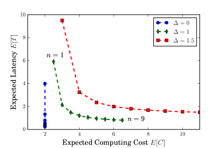
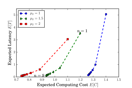
Fig. 5 and Fig. 5 show analytical plots of the expected latency versus cost for log-concave and log-convex respectively. In Fig. 5, the arrival rate , and is shifted exponential , with different values of . For , there is a trade-off between expected latency and cost. Only when , that is, is a pure exponential (which is generally not true in practice), we can reduce latency without any additional cost. In Fig. 5, arrival rate , and is hyperexponential with different values of . We get a simultaneous reduction in and as increases. The cost reduction is steeper as increases.
Instead of holding the arrival rate constant, if we consider that it scales linearly with , then the latency may not always decrease with . In Corollary 3 we study the behavior as varies.
Corollary 3
If the arrival rate , scaling linearly with , then the latency decreases with if is log-convex. If is log-concave then increase with in heavy traffic.
Proof 5.2.
If , then latency in (5) can be rewritten as
| (7) |
If is log-convex then by Lemma 3 we know that decreases with . Similarly, also decreases with (the proof follows similarly as Lemma 3. Hence, we can conclude that the latency in (7) decreases with for log-convex . On the other hand, if is log-concave, then and increase with . Thus, in the heavy traffic regime , when the second term in (7) dominates, increases with .
5.2 Early Task Cancellation
We now analyze the fork-early-cancel system, where we cancel redundant tasks as soon as any task reaches the head of its queue. Intuitively, early cancellation can save computing cost, but the latency could increase due to the loss of diversity advantage provided by retaining redundant tasks. Comparing it to fork-join system, we gain the insight that early cancellation is better when is log-concave, but ineffective for log-convex .
Theorem 7.
The expected latency and cost of the fork-early-cancel system are given by
| (8) | ||||
| (9) |
where is the response time of an queueing system with service time .
Proof 5.3.
In the fork-early-cancel system, when any one tasks reaches the head of its queue, all others are canceled immediately. The redundant tasks help find the queue with the least work left, and exactly one task of each job is served by the first server that becomes idle. Thus, as illustrated in Fig. 6, the latency of the fork-early-cancel system is equivalent in distribution to an queue. Hence and .
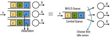
The exact analysis of mean response time has long been an open problem in queueing theory. A well-known approximation given by [Lee and Longton (1959)] is,
| (10) |
where is the expected waiting time in an queueing system with load . This expected waiting time can be evaluated using the Erlang-C model [Harchol-Balter (2013), Chapter 14]. A related work that studies the centralized queue model that the fork-early-cancel system is equivalent to is [Visschers et al. (2012)], which considers the case of heterogeneous job classes with exponential service times.
Next we compare the latency and cost with and without early cancellation given by Theorem 7 and Theorem 6. Corollary 4 below follows from Lemma 3.
Corollary 4
If is log-concave (log-convex), then of the fork-early-cancel system is greater than or equal to (less than or equal to) that of fork-join system.
In the low regime, the fork-join system gives lower than fork-early-cancel because of higher diversity due to redundant tasks. By Corollary 1, in the high regime, the system with lower has lower expected latency.
Corollary 5
If is log-concave, early cancellation gives higher than fork-join when is small, and lower in the high regime. If is log-convex, then early cancellation gives higher for both low and high .
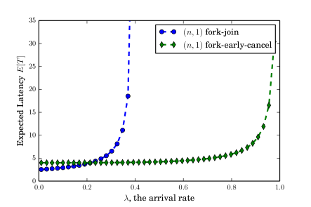
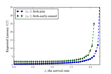
Fig. 8 and Fig. 8 illustrate Corollary 5. Fig. 8 shows a comparison of with and without early cancellation of redundant tasks for the system with service time . We observe that early cancellation gives lower in the high regime. In Fig. 8 we observe that when is which is log-convex, early cancellation is worse for both small and large .
In general, early cancellation is better when is less variable (lower coefficient of variation). For example, a comparison of with fork-join and fork-early-cancel systems as , the constant shift of service time varies indicates that early cancellation is better for larger . When is small, there is more randomness in the service time of a task, and hence keeping the redundant tasks running gives more diversity and lower . But as increases, task service times are more deterministic due to which it is better to cancel the redundant tasks early.
6 PARTIAL FORKING ( CASE)
For applications with a large number of servers , full forking of jobs to all servers can be expensive in terms of the network cost of issuing and canceling the tasks. In this section we analyze the case of the fork-join system, where an incoming job is forked to some out servers and we wait for any task to finish. The servers are chosen using a symmetric policy (Definition 4). Some examples of symmetric policies are:
-
1.
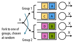
Group-based random: This policy holds when divides . The servers are divided into groups of servers each. A job is forked to one of these groups, chosen uniformly at random.
-
2.
Uniform Random: A job is forked to any out of servers, chosen uniformly at random.
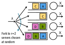
Fig. 9 illustrates the partial-fork-join system with the group-based random and the uniform-random policies. In the sequel, we develop insights into the best and the choice of servers for a given service time distribution .
Remark 8 (Relation to Power-of- Scheduling).
Power-of- scheduling [Mitzenmacher (1996)] is a well-known policy in multi-server systems. It chooses out of the servers at random and assigns an incoming task to the shortest queue among them. A major advantage of the power-of- policy is that even with , the latency achieved by it is close to the join-the-shortest queue policy (equivalent to power-of- with ).
The partial-fork-join system with uniform random policy also chooses queues at random. However, instead of choosing the shortest queue, it creates replicas of the task at all the queues. The replicas help find the queue with the least work left, which gives better load balancing than joining the shortest queue. But unlike power-of-, servers might spend redundant time on replicas that will eventually be canceled.
6.1 Latency-Cost Analysis
In the group-based random policy, the job arrivals are split equally across the groups, and each group behaves like an independent fork-join system. Thus, the expected latency and cost follow from Theorem 6 as given in Lemma 9 below.
Lemma 9 (Group-based random).
The expected latency and cost when each job is forked to one of groups of servers each are given by
| (11) | ||||
| (12) |
Proof 6.1.
The job arrivals are split equally across the groups, such that the arrival rate to each group is a Poisson process with rate . The tasks of each job start service at their respective servers simultaneously, and thus each group behaves like an independent fork-join system with Poisson arrivals at rate . Hence, the expected latency and cost follow from Theorem 6.
Using (12) and Lemma 1, we can infer that the service capacity (maximum supported ) for an system with group-based random policy is
| (13) |
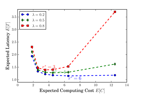
From (13) we can infer that the that minimizes results in the highest service capacity, and hence the lowest in the heavy traffic regime. By Lemma 3, the optimal is () for log-concave (log-convex) . For distributions that are neither log-concave nor log-convex, an intermediate may be optimal and we can determine it using Lemma 9. For example, Fig. 10 shows a plot of latency versus cost as given by Lemma 9 for servers. The task service time . Each job is replicated at servers according to the group-based random policy, with varying along each curve. Initially increasing reduces the latency, but beyond , the replicas cause an increase in the queueing delay. This increase in queueing delay is more dominant for higher . Thus the optimal decreases as increases.
For other symmetric policies, it is difficult to get an exact analysis of and because the tasks of a job can start at different times. However, we can get bounds on depending on the log-concavity of , given in Theorem 10 below.
Theorem 10.
Consider an partial-fork join system, where a job is forked into tasks at out of servers chosen according to a symmetric policy. For any relative task start times , can be bounded as follows.
| (14) | ||||
| (15) |
In the extreme case when , , and when , .
To prove Theorem 10 we take expectation in (4), and show that for log-concave and log-convex , we get the bounds in (14) and (15), which are independent of the relative task start times . The detailed proof is given in Appendix B.
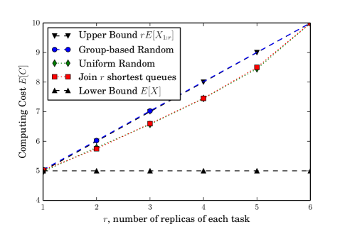
In Fig. 11 we show the bounds given by (14) for log-concave distributions alongside simulation values, for different scheduling policies. The service time , and arrival rate . Since all replicas start simultaneously with the group-based random policy, the upper bound is tight for any . For other scheduling policies, the bound is more loose for the policy that staggers relative start times of replicas to a greater extent.
6.2 Optimal value of
We can use the bounds in Theorem 10 to gain insights into choosing the best when is log-concave or log-convex. In particular, we study two extreme traffic regimes: low traffic () and heavy traffic (), where is the service capacity of the system introduced in Definition 1.
Corollary 6 (Expected Cost vs. )
For a system of servers with symmetric forking of each job to servers, () minimizes the expected cost when is log-concave (log-convex).
The proof follows from Lemma 3, is non-decreasing (non-increasing) with for log-concave (log-convex) .
Lemma 11 (Expected Latency vs. ).
In the low-traffic regime, forking to all servers () gives the lowest for any service time distribution . In the heavy traffic regime, () gives lowest if is log-concave (log-convex).
Proof 6.2.
In the low traffic regime with , the waiting time in queue tends to zero. Thus all replicas of a task start service at the same time, irrespective of the scheduling policy. Then the expected latency is , which decreases with . Thus, gives the lower for any service time distribution .
By Corollary 1, the optimal replication strategy in heavy traffic is the one that minimizes . For log-convex , achieves the lower bound in (15) with equality. Thus, is the optimal strategy in the heavy traffic regime. For log-concave , achieves the lower bound in (14) with equality. Thus, in heavy traffic, gives lowest for log-concave .
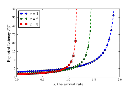
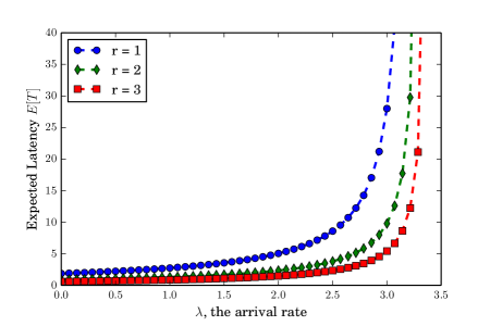
Lemma 11 is illustrated by Fig. 13 and Fig. 13 where calculated analytically using (11) is plotted versus for different values of . Each job is assigned to servers chosen uniformly at random from servers. In Fig. 13 the service time distribution is (which is log-concave) with and . When is small, more redundancy (higher ) gives lower , but in the high regime, gives lowest and highest service capacity. On the other hand in Fig. 13, for a log-convex distribution , in the high load regime decreases as increases.
Lemma 11 was previously proven for new-better-than-used (new-worse-than-used) instead of log-concave (log-convex) in [Shah et al. (2013), Koole and Righter (2008)], using a combinatorial argument. Using Theorem 10, we get an alternative, and arguably simpler way to prove this result. Note that our version is weaker because log-concavity implies new-better-than-used but the converse is not true in general (see Property 3 in Appendix A).
Due to the network cost of issuing and canceling the replicas, there may be an upper limit on the number of replicas. The optimal strategy under this constraint is given by Lemma 12 below.
Lemma 12 (Optimal under ).
For log-convex , is optimal. For log-concave , is optimal in heavy traffic.
The proof is similar to Lemma 11 with replaced by .
6.3 Choice of the servers
For a given , we now compare different policies of choosing the servers for each job. The choice of the servers determines the relative starting times of the tasks. By using the bounds in Theorem 10 that hold for any relative task start times we get the following result.
Lemma 13 (Cost of different policies).
Given , if is log-concave (log-convex), the symmetric policy that results in the tasks starting at the same time ( for all ) results in higher (lower) than one that results in for one or more .
Proof 6.3.
The symmetric policy that results in for all (for eg. the group-based random policy) results in . By Theorem 10, if is log-concave, for any symmetric policy. Thus, for log-concave distributions, the symmetric policy that results in for one or more gives lower than the group-based random policy. On the other hand, for log-convex distributions, with any symmetric policy. Thus the policies that result in relative task start times for all give lower than other symmetric policies.
Lemma 14 (Latency in high regime).
Given , if is log-concave (log-convex), the symmetric policy that results in the tasks starting at the same time ( for all ) results in higher (lower) in the heavy traffic regime than one that results in for some .
Proof 6.4.
By Corollary 1, the optimal replication strategy in heavy traffic is the one that minimizes . Then the proof follows from Lemma 13.
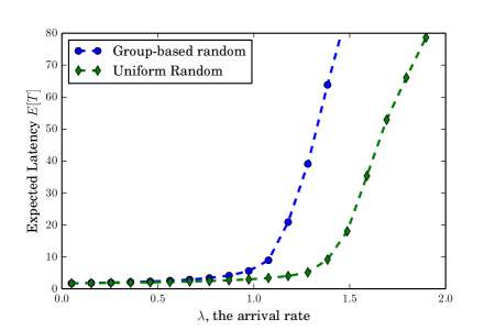
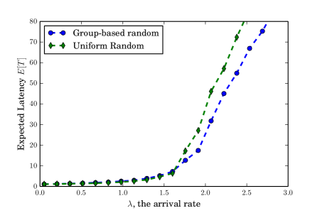
Lemma 14 is illustrated by Fig. 15 and Fig. 15 for and . The simulations are run for workloads with jobs each. The tasks may start at different times with the uniform random policy, whereas they always start simultaneously with group-based random policy. Thus, in the high regime, the uniform random policy results in lower latency for log-concave , as observed in Fig. 15. But for log-convex , group-based forking is better in the high regime as seen in Fig. 15. For low , uniform random policy is better for any because it gives lower expected waiting time in queue.
7 THE GENERAL CASE
We now move to general case, where a job requires any out of tasks to complete. In practice, the general case arises in large-scale parallel computing frameworks such as MapReduce, and in content download from coded distributed storage systems. In this section we present bounds on the latency and cost of the fork-join and fork-early-cancel systems. In Section 7.2 we demonstrate an interesting diversity-parallelism trade-off in choosing .
7.1 Latency and Cost of the fork-join system
Unlike the case, for general exact analysis is hard because multiple jobs can be in service simultaneously (for e.g. Job A and Job B in Fig. 2). Even for the case studied in [Nelson and Tantawi (1988), Varki et al. (2008)], only bounds on latency are known. We generalize those latency bounds to any , and also provide bounds on cost . The analysis of can be used to estimate the service capacity using Lemma 1.
Theorem 15 (Bounds on Latency).
The latency is bounded as follows.
| (16) | ||||
| (17) |
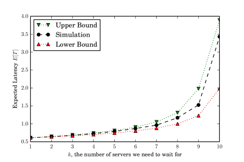
The proof is given in Appendix C. In Fig. 17 we plot the bounds on latency alongside the simulation values for Pareto service time. The upper bound (16) becomes more loose as increases, because the split-merge system considered to get the upper bound (see proof of Theorem 15) becomes worse as compared to the fork-join system. For the special case we can improve the upper bound in Lemma 16 below, by generalizing the approach used in [Nelson and Tantawi (1988)].
Lemma 16 (Tighter Upper bound when ).
For the case , another upper bound on latency is given by,
| (18) |
where are i.i.d. realizations of the response time of an queue with arrival rate , service time distribution .
The proof is given in Appendix C. Transform analysis [Harchol-Balter (2013), Chapter 25] can be used to determine the distribution of , the response time of an queue in terms of . The Laplace-Stieltjes transform of the probability density function of of is given by,
| (19) |
where is the Laplace-Stieltjes transform of the service time distribution .
The lower bound on latency (17) can be improved for shifted exponential , generalizing the approach in [Varki et al. (2008)] based on the memoryless property of the exponential tail.
Theorem 17 (Bounds on Cost).
The expected computing cost can be bounded as follows.
| (20) | ||||
| (21) |
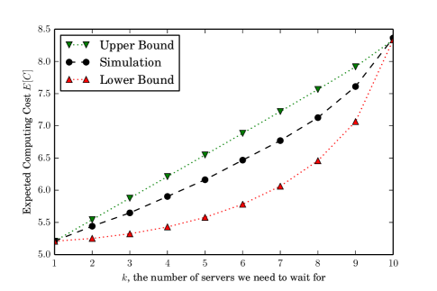
The proof is given in Appendix C. Fig. 17 shows the bounds alongside the simulation plot of the computing cost when is with and . The arrival rate , and with varying from to on the x-axis. The simulation is run for iterations of jobs. We observe that the bounds on are tight for and , which can also be inferred from (20) and (21).
7.2 Diversity-Parallelism Trade-off
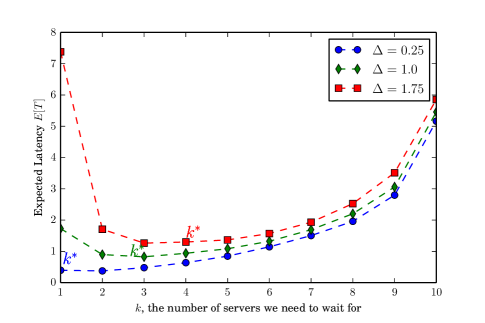
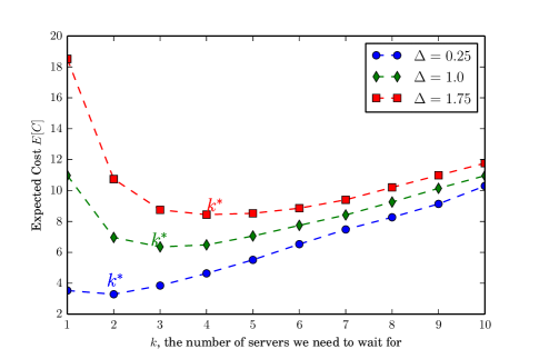
In Fig. 17 we observed the expected latency increases with , because we need to wait for more tasks to complete, and the service time is independent of . But in most computing and storage applications, the service time decreases as increases because each task becomes smaller. We refer to this as the ‘parallelism benefit’ of splitting a job into more tasks. But as increases, we lose the ‘diversity benefit’ provided by redundant tasks and having to wait only for a subset of the tasks to finish. Thus, there is a diversity-parallelism trade-off in choosing the optimal that minimizes latency . We demonstrate the diversity-parallelism trade-off in simulation plot Fig. 19 for service time , with , and . As increases, we lose diversity but the parallelism benefit is higher because each task is smaller. As increases, the optimal shifted upward because the service time distribution becomes ‘less random’ and so there is less diversity benefit.
We can also observe the diversity-parallelism trade-off mathematically in the low traffic regime, for . If we take in (17) and (16), both bounds coincide and we get,
| (22) |
where , the harmonic number. The parallelism benefit comes from the first term in (22), which reduces with . The diversity of waiting for out of tasks causes the second term to increase with . The optimal that minimizes (22) strikes a balance between these two opposing trends.
Fig. 19 shows a similar diversity-parallelism trade-off in choosing to minimize the computing cost . In the heavy traffic regime, by Corollary 1 the policy that minimizes also minimizes . Thus the same will minimize both and .
7.3 Latency and Cost of the fork-early-cancel system
We now analyze the latency and cost of the fork-early-cancel system where the redundant tasks are canceled as soon as any tasks start service.
Theorem 18 (Latency-Cost with Early Cancellation).
The cost and an upper bound on the expected latency with early cancellation is given by
| (23) | ||||
| (24) |
where are i.i.d. realizations of , the reponse time of an queue with arrival rate and service time distribution .
The proof is given in Appendix C. The Laplace-Stieltjes transform of the response time of an queue with service time distribution and arrival rate is same as (19), with replaced by .
By comparing the cost in (23) to the bounds in Theorem 17 without early cancellation, we can get insights into when early cancellation is effective for a given service time distribution . For example, when is log-convex, the upper bound in (20) is smaller than . Thus we can infer that the fork-early-cancel system is always worse than the fork-join system when is log-convex. We also observed this phenomenon in Fig. 8 for the case.
8 GENERAL REDUNDANCY STRATEGY
From the analysis in Section 5 and Section 6, we get insights into designing the best redundancy strategy for log-concave and log-convex service time. But it is not obvious to infer the best strategy for arbitrary service time distributions, or when only empirical traces of the service time are given. We now propose such a redundancy strategy to minimize the latency, subject to computing and network cost constraints. This strategy can also be used on traces of task service time when closed-form expressions of and its order statistics are not known.
8.1 Generalized Fork-join Model
We first introduce a general fork-join variant that is a combination of the partial fork introduced in Section 2, and partial early cancellation of redundant tasks.
Definition 19 ( fork-join system).
For a system of servers and a job that requires tasks to complete, we do the following:
-
•
Fork the job to out of the servers chosen uniformly at random.
-
•
When any tasks are at the head of queues or in service already, cancel all other tasks immediately. If more than tasks start service simultaneously, retain randomly chosen ones out of them.
-
•
When any tasks finish, cancel all remaining tasks immediately.
Note tasks may finish before some start service, and thus we may not need to perform the partial early cancellation in the second step above.
Recall that the servers have service time distribution that is i.i.d. across the servers and tasks. The tasks that are canceled early, help find the shortest out of the queues, thus reducing waiting time. From the tasks retained, waiting for any to finish provides diversity and hence reduces service time.
The special cases , and correspond to the fork-join and fork-early-cancel and partial-fork-join systems respectively, which are defined in Section 2.
8.2 Choosing Parameters and
We propose a strategy to choose and to minimize expected latency , subject to a computing cost constraint is , and a network cost constraint is . We impose the second constraint because forking to more servers results in higher network cost of remote-procedure-calls (RPCs) to launch and cancel the tasks.
Definition 20 (Proposed Redundancy Strategy).
Choose and to minimize subject to constraints and . The solutions are
| (25) | ||||
| (26) |
where and are estimates of the expected latency and cost , defined as follows:
| (27) | ||||
| (28) |
To justify the strategy above, observe that for a given , increasing gives higher diversity in finding the queues with the least-work-left and thus reduces latency. Since tasks are canceled early before starting service, affects only mildly, through the relative task start times of tasks that are retained. So we conjecture that it is optimal to set in (25), the maximum value possible under network cost constraints. Changing on the other hand does affect both the computing cost and latency significantly. Thus to determine the optimal , we minimize subject to constraints and as given in (26).
The estimates and are obtained by generalizing Lemma 9 for group-based random forking to any , and that may not divide . When the order statistics of are hard to compute, or itself is not explicitly known, and can be also be found using empirical traces of .
The sources of inaccuracy in the estimates and are as follows.
-
1.
For , the latency estimate is a generalization of the split-merge queueing upper bound in Theorem 15. Since the bound becomes loose as increases, the error increases with .
-
2.
The estimates and are by definition independent of , which is not true in practice. As explained above, for , the actual is generally less than , and can be slightly higher or lower than .
-
3.
Since the estimates and are based on group-based forking, they consider that all tasks start simultaneously. Variability in relative task start times can result in actual latency and cost that are different from the estimates. For example, from Theorem 10 we can infer that when is log-concave (log-convex), the actual computing cost is less than (greater than) .
The factor (1) above is the largest source of inaccuracy, especially for larger and . Since the estimate is an upper bound on the actual latency, the and recommended by the strategy are smaller than or equal to their optimal values. Factors (2) and (3) only affect the relative task start times and generally result in a smaller error in estimating and .
8.3 Simulation Results
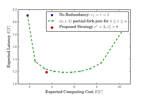
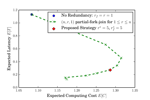
We now present simulation results comparing the proposed strategy given in Definition 20 to the partial-fork-join system with varying from to . The service time distributions considered here are neither log-concave nor log-convex, thus making it hard to directly infer the best redundancy strategy using the analysis presented in the previous sections. The simulations are run for workloads with jobs each.
In Fig. 21 the service time , , , and arrival rate . The computing and network cost constraints are and respectively. We observe that the proposed strategy gives a significant latency reduction as compared to the no redundancy case ( in the partial-fork-join system). We observe that the proposed strategy gives a latency-cost trade-off that is better than the partial-fork-join system. Using partial early cancellation () gives an additional reduction in latency by providing greater diversity and helping us find the out of queues with the least work left.
In Fig. 21 we show a case where the cost does not always increase with the amount of redundancy . The task service time is a mixture of an exponential and a shifted exponential , each occurring with equal probability. The other parameters are , , and arrival rate . The proposed strategy found using Definition 20 is , limited by the constraint rather than the constraint. Since , it coincides exactly with the partial-fork-join system.
9 CONCLUDING REMARKS
In this paper we consider a redundancy model where each incoming job is forked to queues at multiple servers and we wait for any one replica to finish. We analyze how redundancy affects the latency, and the cost of computing time, and demonstrate how the log-concavity of service time is a key factor affecting the latency-cost trade-off. Some key insights from this analysis are:
-
•
For log-convex service times, forking to more servers (more redundancy) reduces both latency and cost. On the other hand, for log-concave service times, more redundancy can reduce latency only at the expense of an increase in cost.
-
•
Early cancellation of redundant requests can save both latency and cost for log-concave service time, but it is not effective for log-convex service time.
Using these insights, we also propose a general redundancy strategy for an arbitrary service time distribution, that may be neither log-concave nor log-convex. This strategy can also be used on empirical traces of service time, when a closed-form expression of the distribution is not known.
Ongoing work includes developing online strategies to simultaneously learn the service time distribution, and the best redundancy strategy. More broadly, the proposed redundancy techniques can be used to reduce latency in several applications beyond the realm of cloud storage and computing systems, for example crowdsourcing, algorithmic trading, manufacturing etc.
10 ACKNOWLEDGMENTS
We thank Da Wang, Devavrat Shah, Sem Borst and Rhonda Righter for helpful dicussions. We also thank anonymous reviews for valuable feedback that helped improve this work.
APPENDIX
Appendix A LOG-CONCAVITY OF
In this section we present some properties and examples of log-concave and log-convex random variables that are relevant to this work. For more properties please see [Bagnoli and Bergstrom (2005)].
Property 1 (Jensen’s Inequality)
If is log-concave, then for and for all ,
| (29) |
The inequality is reversed if is log-convex.
Proof A.1.
Since is log-concave, is concave. Taking on both sides on (29) we get the Jensen’s inequality which holds for concave functions.
In past literature saying is log-concave usually means that is log-concave. This implies that and . However log-convex , does not always imply log-convexity of and .
Property 2 (Scaling)
If is log-concave, for ,
| (30) |
The inequality is reversed if is log-convex.
Proof A.2.
Property 3 (Sub-multiplicativity)
If is log-concave, the conditional tail probability of satisfies for all ,
| (33) | ||||
| (34) |
The inequalities above are reversed if is log-convex.
Proof A.3.
| (35) | |||
| (36) | |||
| (37) |
where we apply Property 2 to (36) to get (37). Equation (33) follows from (37).
Note that for exponential which is memoryless, (33) holds with equality. Thus log-concave distributions can be thought to have ‘optimistic memory’, because the conditional tail probability decreases over time. On the other hand, log-convex distributions have ‘pessimistic memory’ because the conditional tail probability increases over time. The definition of the notions ‘new-better-than-used’ in [Koole and Righter (2008)] is same as (33). By Property 3 log-concavity of implies that is new-better-than-used. New-better-than-used distributions are referred to as ‘light-everywhere’ in [Shah et al. (2013)] and ‘new-longer-than-used’ in [Sun et al. (2015)].
Property 4 (Mean Residual Life)
If is log-concave (log-convex), , the mean residual life after time has elapsed is non-increasing (non-decreasing) in .
Proof A.4 (of Lemma 3).
Lemma 3 is true for log-concave if for all integers . This inequality can be simplified as follows.
| (38) | ||||
| (39) | ||||
| (40) | ||||
| (41) |
We get (39) using the fact that the expected value of a non-negative random variable is equal to the integral of its tail distribution. To get (40) observe that since for i.i.d. , we have for all . Similarly . Next we perform a change of variables on both sides of (40) to get (41).
Now we use Property 2 to compare the two integrands in (41). Setting and in Property 2, we get
| (42) |
Property 5 (Hazard Rates)
If is log-concave (log-convex), then the hazard rate , which is defined by , is non-decreasing (non-increasing) in .
Property 6 (Coefficient of Variation)
The coefficient of variation is the ratio of the standard deviation and mean of random variable . For log-concave (log-convex) , (), and when is pure exponential.
Property 7 (Examples of Log-concave )
The following distributions have log-concave :
-
•
Shifted Exponential (Exponential plus constant )
-
•
Uniform over any convex set
-
•
Weibull with shape parameter
-
•
Gamma with shape parameter
-
•
Chi-squared with degrees of freedom
Property 8 (Examples of Log-convex )
The following distributions have log-convex :
-
•
Exponential
-
•
Hyper Exponential (Mixture of exponentials)
-
•
Weibull with shape parameter
-
•
Gamma with shape parameter
Appendix B PROOFS FOR THE Case
Proof B.1 (of Theorem 10).
Using (4), we can express the cost in terms of the relative task start times , and as follows. Since only tasks are invoked, the relative start times are equal to .
| (43) |
where is the time between the start of service of the earliest task, and when any of the tasks finishes. The tail distribution of is given by
| (44) |
By taking expectation on both sides of (43) and simplifying we get,
| (45) | ||||
| (46) | ||||
| (47) | ||||
| (48) |
We now prove that for log-concave , . The proof that when is log-convex follows similarly with all inequalities below reversed. We express the integral in (48) as,
| (49) | ||||
| (50) | ||||
| (51) | ||||
| (52) |
where in (49) we express each integral in (48) as a difference of two integrals from to . In (50) we perform a change of variables . In (51) we rearrange the grouping of the terms in the sum; the negative integral is put in the term of the summation. Then the first term of the summation is simply which is equal to . In (51) we use the fact that each term in the summation in (50) is positive when is log-concave. This is shown in Lemma 21 below.
Next we prove that for log-concave , . Again, the proof of when is log-convex follows with all the inequalities below reversed.
| (53) | ||||
| (54) | ||||
| (55) | ||||
| (56) |
where we get (53) by applying Property 2 to (48). In (54) we express the integral as a difference of two integrals from to , and perform a change of variables . In (55) we rearrange the grouping of the terms in the sum; the negative integral is put in the term of the summation. The first term is equal to . We use Lemma 22 to show that each term in the summation in (55) is negative when is log-concave.
Lemma 21.
If is log-concave,
| (57) |
The inequality is reversed for log-convex .
Proof B.2 (of Lemma 21).
We bound the left hand side expression as follows.
| (58) | ||||
| (59) | ||||
| (60) | ||||
| (61) | ||||
| (62) |
where we use Property 3 to get (60). The inequality in (61) follows from applying Property 2 to the conditional distribution , which is also log-concave.
For log-convex all the inequalities can be reversed.
Lemma 22.
If is log-concave,
| (63) |
The inequality is reversed for log-convex .
Appendix C PROOFS FOR GENERAL
Proof C.1 (of Theorem 15).
To find the upper bound on latency, we consider a related queueing system called the split-merge queueing system. In the split-merge system all the queues are blocked and cannot serve subsequent jobs until out of tasks of the current job are complete. Thus the latency of the split-merge system serves as an upper bound on that of the fork-join system. In the split-merge system we observe that jobs are served one-by-one, and no two jobs are served simultaneously. So it is equivalent to an queue with Poisson arrival rate , and service time . The expected latency of an queue is given by the Pollaczek-Khinchine formula [Gallager (2013), Chapter 5], and it reduces to the upper bound in (16).
To find the lower bound we consider a system where the job requires out of tasks to complete, but all jobs arriving before it require only task to finish. Then the expected waiting time in queue is equal to the second term in (16) with set to . Adding the expected service time to this lower bound on expected waiting time, we get the lower bound (17) on the expected latency.
Proof C.2 (of Lemma 16).
This upper bound is a generalization of the bound on the mean response time of the fork-join system with exponential service time presented in [Nelson and Tantawi (1988)]. To find the bound, we first observe that the response times experienced by the tasks in the queues form a set of associated random variables [Esary et al. (1967)]. Then we use the property of associated random variables that their expected maximum is less than that for independent variables with the same marginal distributions. Unfortunately, this approach cannot be extended to the case because this property of associated variables does not hold for the order statistic for .
Proof C.3 (of Theorem 17).
A key observation used in proving the cost bounds is that at least out of the tasks of a job start service at the same time. This is because when the task of Job finishes, the remaining tasks are canceled immediately. These queues start working on the tasks of Job at the same time.
To prove the upper bound we divide the tasks into two groups, the tasks that can start early, and the which start at the same time after the last tasks of the previous job are terminated. We consider a constraint that all the tasks in the first group and of the remaining tasks needs to be served for completion of the job. This gives an upper bound on the computing cost because we are not taking into account the case where more than one tasks from the second group can finish service before the tasks in the first group. For the tasks in the second group, the computing cost is equal to times the time taken for one of them to complete. The computing time spent on the first tasks is at most . Adding this to the second group’s cost, we get the upper bound (20).
We observe that the expected computing cost for the tasks that finish is at least , which takes into account full diversity of the redundant tasks. Since we need tasks to complete in total, at least of the tasks that start simultaneously needs to be served. Thus, the computing cost of the redundant tasks is at least . Adding this to the lower bound on the first group’s cost, we get (21).
Proof C.4 (of Theorem 18).
Since exactly tasks are served, and others are cancelled before they start service, it follows that the expected computing cost . In the sequel, we find an upper bound on the latency of the fork-early-cancel system.
First observe that in the fork-early-cancel system, the redundant tasks that are canceled early help find the shortest queues. The expected task arrival rate at each server is , which excludes the redundant tasks that are canceled before they start service.
Consider an partial fork system without redundancy, where the tasks of each job are assigned to out of queues chosen uniformly at random. The job exits the system when all tasks are complete. The expected task arrival rate at each server is , same as the fork-early-cancel system. However, the fork-early-cancel system gives lower latency because having the redundant tasks provides diversity and helps find the shortest queues. Thus the latency of the partial-fork-join system is bounded below by that of the fork-early-cancel system.
Now let us upper bound the latency of the partial fork system. Each queue has arrival rate , and service time distribution . Using the approach in [Nelson and Tantawi (1988)] we can show that the response times (waiting plus service time) , of the queues serving each job form a set of associated random variables. Then by the property that the expected maximum of associated random variables is less than the expected maximum of independent variables with the same marginal distributions we can show that,
| (67) | ||||
| (68) |
The expected maximum can be numerically evaluated from distribution of . From the transform analysis given in [Harchol-Balter (2013), Chapter 25], we know that the Laplace-Stieltjes transform of the probability density of is same as (19), but with replaced by .
References
- Ananthanarayanan et al. (2013) Ananthanarayanan, G., Ghodsi, A., Shenker, S., and Stoica, I. 2013. Effective straggler mitigation: Attack of the clones. In USENIX Conference on Networked Systems Design and Implementation. 185–198.
- Bagnoli and Bergstrom (2005) Bagnoli, M. and Bergstrom, T. 2005. Log-concave probability and its applications. Economic Theory 26, 2, pp. 445–469.
- Cao and Wang (1991) Cao, J. and Wang, Y. 1991. The nbuc and nwuc classes of life distributions. Journal of Applied Probability, 473–479.
- Chen et al. (2014) Chen, S., Kozat, U. C., Huang, L., Sinha, P., Liang, G., Liu, X., Sun, Y., and Shroff, N. B. 2014. When Queueing Meets Coding: Optimal-Latency Data Retrieving Scheme in Storage Clouds. IEEE International Conference on Communications.
- Dean and Barroso (2013) Dean, J. and Barroso, L. 2013. The Tail at Scale. Communications of the ACM 56, 2, 74–80.
- Dean and Ghemawat (2008) Dean, J. and Ghemawat, S. 2008. MapReduce: simplified data processing on large clusters. ACM Commun. Mag. 51, 1, 107–113.
- Esary et al. (1967) Esary, J., Proschan, F., and Walkup, D. 1967. Association of random variables, with applications. Annals of Mathematics and Statistics 38, 5, 1466–1474.
- Flatto and Hahn (1984) Flatto, L. and Hahn, S. 1984. Two parallel queues created by arrivals with two demands I. SIAM Journal on Applied Mathematics 44, 5, 1041–1053.
- Gallager (2013) Gallager, R. 2013. Stochastic Processes: Theory for Applications 1st Ed. Cambridge University Press.
- Gardner et al. (2015) Gardner, K., Zbarsky, S., Doroudi, S., Harchol-Balter, M., Hyytiä, E., and Scheller-Wolf, A. 2015. Reducing latency via redundant requests: Exact analysis. In ACM SIGMETRICS.
- Harchol-Balter (2013) Harchol-Balter, M. 2013. Performance Modeling and Design of Computer Systems: Queueing Theory in Action. Cambridge University Press.
- Joshi et al. (2012) Joshi, G., Liu, Y., and Soljanin, E. 2012. Coding for fast content download. Allerton Conf. on Communication, Control and Computing, 326–333.
- Joshi et al. (2014) Joshi, G., Liu, Y., and Soljanin, E. 2014. On the Delay-storage Trade-off in Content Download from Coded Distributed Storage. IEEE Journal on Selected Areas on Communications.
- Joshi et al. (2015) Joshi, G., Soljanin, E., and Wornell, G. 2015. Queues with redundancy: Latency-cost analysis. In ACM SIGMETRICS Workshop on Mathematical Modeling and Analysis.
- Kabatiansky et al. (2005) Kabatiansky, G., E., K., and S., S. 2005. Error correcting coding and security for data networks: analysis of the superchannel concept 1st Ed. Wiley, Chapter 7.
- Kadhe et al. (2015) Kadhe, S., Soljanin, E., and Sprintson, A. 2015. Analyzing the download time of availability codes. International Symposium on Information Theory (ISIT).
- Kim et al. (2009) Kim, Y., Righter, R., and Wolff, R. 2009. Job replication on multiserver systems. Advances in Applied Probability 41, 2, pp. 546–575.
- Koole and Righter (2008) Koole, G. and Righter, R. 2008. Resource allocation in grid computing. Journal of Scheduling 11, 3, 163–173.
- Kumar et al. (2014) Kumar, A., Tandon, R., and Clancy, T. C. 2014. On the latency of heterogeneous mds queue. In IEEE Global Communications Conference (GLOBECOM). 2375–2380.
- Lee and Longton (1959) Lee, A. M. and Longton, P. A. 1959. Queueing process associated with airline passenger check-in. Operations Research Quarterly, 56–71.
- Liang and Kozat (2014) Liang, G. and Kozat, U. 2014. TOFEC: Achieving Optimal Throughput-Delay Trade-off of Cloud Storage Using Erasure Codes. IEEE International Conference on Communications.
- Maxemchuk (1975) Maxemchuk, N. F. 1975. Dispersity routing. International Conference on Communications (ICC), 41.10–41.13.
- Mitzenmacher (1996) Mitzenmacher, M. 1996. The power of two choices in randomized load balancing. Ph.D. thesis, University of California Berkeley, CA.
- Nelson and Tantawi (1988) Nelson, R. and Tantawi, A. 1988. Approximate analysis of fork/join synchronization in parallel queues. 37, 6, 739–743.
- Ousterhout et al. (2013) Ousterhout, K., Wendell, P., Zaharia, M., and Stoica, I. 2013. Sparrow: Distributed, low latency scheduling. In ACM Symposium on Operating Systems Principles (SOSP). 69–84.
- Shah et al. (2014) Shah, N., Lee, K., and Ramachandran, K. 2014. The mds queue: Analyzing the latency performance of erasure codes. IEEE International Symposium on Information Theory.
- Shah et al. (2013) Shah, N., Lee, K., and Ramchandran, K. 2013. When do redundant requests reduce latency? In Allerton Conf. on Comm., Control and Computing.
- Sun et al. (2015) Sun, Y., Zheng, Z., Koksal, C. E., Kim, K., and Shroff, N. B. 2015. Provably delay efficient data retrieving in storage clouds. In IEEE Conference on Computer Communications (INFOCOM).
- Varki et al. (2008) Varki, E., Merchant, A., and Chen, H. 2008. The M/M/1 fork-join queue with variable sub-tasks. unpublished, available online..
- Visschers et al. (2012) Visschers, J., Adan, I., and Weiss, G. 2012. A product form solution to a system with multi-type jobs and multi-type servers. Queueing Systems 70, 3, 269–298.
- Vulimiri et al. (2013) Vulimiri, A., Godfrey, P. B., Mittal, R., Sherry, J., Ratnasamy, S., and Shenker, S. 2013. Low latency via redundancy. In ACM Conference on Emerging Networking Experiments and Technologies. CoNEXT ’13. ACM, 283–294.
- Wang et al. (2014) Wang, D., Joshi, G., and Wornell, G. 2014. Efficient task replication for fast response times in parallel computation. ACM Sigmetrics short paper.
- Wang et al. (2015) Wang, D., Joshi, G., and Wornell, G. 2015. Using straggler replication to reduce latency in large-scale parallel computing (extended version). arXiv:1503.03128 [cs.dc].
- Xiang et al. (2014) Xiang, Y., Lan, T., Aggarwal, V., and Chen, Y. F. R. 2014. Joint latency and cost optimization for erasure-coded data center storage. SIGMETRICS Performance Evaluation Review 42, 2, 3–14.