Short relaxation times but long transient times in both simple and complex reaction networks

Abstract

When relaxation towards an equilibrium or steady state is exponential at large times, one usually considers that the associated relaxation time $\tau$, i.e., the inverse of that decay rate, is the longest characteristic time in the system. However that need not be true, and in particular other times such as the lifetime of an infinitesimal perturbation can be much longer. In the present work we demonstrate that this paradoxical property can arise even in quite simple systems such as a chain of reactions obeying mass action kinetics. By mathematical analysis of simple reaction networks, we pin-point the reason why the standard relaxation time does not provide relevant information on the potentially long transient times of typical infinitesimal perturbations. Overall, we consider four characteristic times and study their behavior in both simple chains and in more complex reaction networks taken from the publicly available database “Biomodels”. In all these systems involving mass action rates, Michaelis-Menten reversible kinetics, or phenomenological laws for reaction rates, we find that the characteristic times corresponding to lifetimes of tracers and of concentration perturbations can be much longer than $\tau$.

I Introduction

Networks have been used to model systems involving large numbers of components, agents, or species Albert and Barabási (2002). Of particular interest are the effects arising in such systems either because of out-of-equilibrium dynamics or through equilibrium phase transitions. Collective effects are generally associated with slow dynamics, i.e., characteristic times that are much larger than the microscopic times associated with elementary processes. In the present work our focus is on the emergence of large characteristic times in reaction networks close to their steady state. There are many ways to define a characteristic time in a dynamical system. The simplest is via the asymptotic relaxation towards the steady state Awazu and Kaneko (2009); Jamshidi and Palsson (2008), relaxation which often will be exponential. If so, the amplitude of the perturbation or “distance” to the steady state will decay as $\exp(-t/\tau)$ at very long times, from which one then defines $\tau$ to be the relaxation time. Although in familiar situations $\tau$ is the longest characteristic time, our goal here is to investigate cases where much larger times can arise. Our study focuses on reaction networks for specificity, but our framework is generally applicable to any system.

Reaction networks involve species that can transform one into another. If the species are molecular, one can get insights into the dynamics of the system by introducing an isotopic tracer and by following in time its incorporation into the different molecular species Meier et al. (2011). Assume that the reaction network is in contact with outside reservoirs, and let $t_{t}$ be the time the tracer takes to exit the system. Surprisingly, the mean of $t_{t}$, corresponding to the lifetime Hardt (1981); Waniewski (2007) of the tracer (and sometimes called the mean residence time of the tracer), can be much greater than $\tau$. The object of our work is to understand such a possibility, pointing in particular to the danger of assuming that $\tau$ is the main and longest characteristic time in these systems. For pedagogical reasons, we will begin by treating one-dimensional networks because an in-depth analytical treatment is feasible there, from which one can easily understand the influence of network size. We will then study more general systems using reaction networks published by other authors. In all cases, we compare the behaviors of four characteristic times in these systems, investigating the causes that can render them non informative or make their ratios diverge.

II Models and Methods

II.1 Networks, molecular species and associated reactions

A metabolic network consists of a set of reactions and associated metabolites. It is convenient to represent such a network as a graph where the nodes are associated with metabolites; these are linked together by edges when there is a reaction that includes them as substrate and product. Such edges may be uni or bi-directional, accounting for the reversibility of the associated reaction. Let there be $N$ metabolites $M_{i}$ ($i=1,...,N)$ and define $C_{i}$ as the concentration of $M_{i}$. We are interested in the dynamics of the $C_{i}$, i.e., how these quantities change with time and in the corresponding fluxes through the different reactions. Specifically, we shall study the dynamics close to the system’s steady state and we shall probe the associated characteristic times. To facilitate the mathematical understanding of these times, we shall first focus on a particular kind of network consisting of a linear chain of reactions. In that situation, we order the metabolites from $0$ to $N+1$ where the metabolite $M_{i}$ is the product of reaction $R_{i}$ whose substrate is metabolite $M_{i-1}$:

$${M_{0}}\overset{v_{1}}{\leftrightarrow}M_{1}\overset{v_{2}}{\leftrightarrow}...\overset{v_{N}}{\leftrightarrow}M_{N}\overset{v_{N+1}}{\leftrightarrow}{M_{N+1}}$$ (1)

The metabolites ${M_{0}}$ and ${M_{N+1}}$ reside in infinite reservoirs at the two extremities of the chain so their concentrations are constant. By convention, the forward direction in such a chain goes from $M_{0}$ to $M_{N+1}$. Once understood the characteristic times in this system, we shall use the insight thereby gained to probe the situation in more realistic metabolic networks having branches and loops.

Reactions transform metabolites into other metabolites but it is necessary still to specify the actual kinetics. When a reaction happens spontaneously, without the need for a catalyst, it can be modeled by a mass action rate law (MA) where the flux is given by

$$v^{MA}_{i}=a_{i}C_{i-1}-b_{i}C_{i}\,.$$ (2)

To be specific, one can consider using the usual convention whereby concentrations are measured in Moles per liter and fluxes in Moles per liter per second. The parameter $a_{i}$ (resp. $b_{i}$) is then the probability per second that a molecule of metabolite $M_{i-1}$ (resp. $M_{i}$) spontaneously transforms into a molecule of metabolite $M_{i}$ (resp. $M_{i-1}$). Note that Eq. 2 gives the total flux which is the forward flux minus the backward flux.

In practice, one is often interested in catalyzed reactions where the spontaneous rates are terribly low. For instance, in biochemistry, most reactions are catalyzed by enzymes; the catalysis allows for rates that can be enhanced by a factor of $10^{10}$ or more. For any such enzymatic reaction, the rate may be limited by the amount of enzyme and is no longer directly proportional to metabolite concentration. Generally, the relation between substrate concentration and reaction rate grows linearly at low concentrations and then saturates at high concentrations of substrate. The reaction kinetics in this situation are typically modeled by the so called reversible Michaelis-Menten-Henri ($MMH$) law Haldane (1930). In the case of a reaction involving one substrate and one product, the flux is given by

$$v^{MMH}_{i}=\frac{\alpha_{i}\frac{C_{i-1}}{K_{S}^{i}}-\beta_{i}\frac{C_{i}}{K_{P}^{i}}}{1+\frac{C_{i-1}}{K_{S}^{i}}+\frac{C_{i}}{K_{P}^{i}}}\,.$$ (3)

Here, $\alpha_{i}$ is the maximum rate in the forward direction, reached when the substrate is in large excess and the product is absent. Similarly, $\beta_{i}$ is the maximum rate in the backward direction. The maximum forward rate is proportional to the enzyme concentration and is often decomposed as $\alpha=k_{cat}E$ with $E$ being the enzyme concentration and $k_{cat}$ the maximum number of reactions catalyzed by one molecule of enzyme per unit of time. $K_{S}^{i}$ and $K_{P}^{i}$, called the Michaelis constants respectively for substrate and product, are characteristic concentrations which set the scale for when the reaction becomes saturated in substrate or in product. For a $MMH$ reaction in the absence of the product, $K_{S}$ is the concentration for which the rate is at half of its maximum value.

II.2 Determining steady states

When a physical system is not driven by outside forces, it goes to its equilibrium state where all net reaction fluxes are 0. In the context of our one dimensional model, that can only arise if the free energies of the two reservoirs are equal, corresponding to tuning the concentrations so that their ratio is the equilibrium one. Outside of that special case, the system will be out of equilibrium and concentrations will change in time until a steady state is reached which necessarily will have non zero fluxes. This steady state is generally unique if there are no regulatory processes but for our study to be completely general, we will not assume uniqueness of the steady state, we shall simply consider a stable steady state and investigate its characteristic times.

We have followed two approaches for determining steady states (leading to identical results):

1. solve the steady state equations $dC_{i}/dt=0$ which we do numerically using root finding (routine “find-root” in Python). For any given boundary conditions, i.e., concentrations $C_{0}$ and $C_{N+1}$, this leads to a list of steady-state concentrations $\overrightarrow{C^{ss}}$. It is necessary to check that the resulting steady state is linearly stable. This check can be performed using the linearized equations about the steady state. If $\overrightarrow{\delta C}$ is the (infinitesimal) difference between the actual concentrations and those in the steady state, one has

   $$\frac{d\overrightarrow{\delta C}}{dt}=\mathbb{J^{(c)}}\overrightarrow{\delta C}$$ (4)

   $$\mathbb{J^{(c)}}_{ij}=\begin{cases}A_{i}\quad\mbox{if}\quad j=i-1\\ -(A_{i+1}+B_{i})\quad\mbox{if}\quad j=i\\ B_{i+1}\quad\mbox{if}\quad j=i+1\\ 0\quad\mbox{otherwise}\end{cases}\,$$ (5)

   where the $A_{i}$ and $B_{i}$ are related to the terms entering Eq. 2 for mass action and Eq. 3 for Michaelis Menten Henri as specified in Table 1. $\mathbb{J^{(c)}}$ is the $N\times N$ Jacobian matrix with indices $i$ and $j$ going from 1 to $N$; the superscript $c$ refers to the fact that it describes the (linearized) dynamics of (perturbed) concentrations. The steady state is stable if all the eigenvalues of the Jacobian have negative real part.

2. follow the concentrations using the dynamical equations (the system of ordinary differential equations specified by the kinetic laws) and extract the long time limit of the concentrations. This requires extrapolation, but generically takes one to a stable steady state.

II.3 Defining four characteristic times

• The first characteristic time is the relaxation time defined as $-1/\lambda_{1}^{(c)}$ where $\lambda_{1}^{(c)}$ is the real part of the leading eigenvalue of $\mathbb{J^{(c)}}$ having the largest real part. Because this time is defined via the linearized dynamics for the concentrations about the steady state, we shall refer to it as $\tau_{c}$.

• The second characteristic time is the previously mentioned tracer lifetime (or mean residence time), which we denote by $T_{t}$. The motivation for introducing this quantity comes from tracer experiments in chemical networks where isotopic labels are used to follow atoms as reactions progress. Instead of introducing a perturbation to concentrations, this approach labels (e.g. via an NMR pulse) atoms of one metabolite $M_{k}$ at $t=0$ without changing any concentrations. In practice this labeling affects only a fraction of the molecules. The effect of this labeling is to leave the fluxes unperturbed as well. The system stays in its steady state, it is just that some of these concentrations become labeled. Note that when one labeled metabolite is tranformed into another, the labeling follows because the labeled atoms.

  Let us study the time evolution of the concentrations of these tracers $\overrightarrow{C_{t}}=\{C_{t,1},C_{t,2},\ldots,C_{t,N}\}$ (the subscript $t$ is for tracer). As previously introduced, let $\overrightarrow{C^{ss}}=\{C^{ss}_{1},C^{ss}_{2},\ldots,C^{ss}_{N}\}$ be the steady state concentrations. Consider the reaction $R_{i}$ and let ${\phi^{f}}_{i}$ be its forward flux and ${\phi^{b}}_{i}$ its backward flux in the steady state. Then the labeled concentration $C_{t,i}$ will include an incoming term given by the rescaled forward flux ${\phi^{f}}_{i}\,C_{t,i-1}/C^{ss}_{i-1}$ because all metabolite molecules (labeled or not) have an equal probability of participating in the reaction $R_{i}$. As a result, the dynamics of the tracer concentrations is

  $$\frac{d\overrightarrow{C_{t}}}{dt}=\mathbb{J^{(t)}}\overrightarrow{C_{t}}$$ (6)

  $$\mathbb{J^{(t)}}_{ij}=\begin{cases}\phi^{f}_{i}/C^{ss}_{j}\quad\mbox{if}\quad j=i-1\\ -(\phi^{f}_{i}/C^{ss}_{i-1}+\phi^{b}_{i-1}/C^{ss}_{i-1})\quad\mbox{if}\quad j=i\\ \phi^{b}_{i}/C^{ss}_{i}\quad\mbox{if}\quad j=i+1\\ 0\quad\mbox{otherwise}\end{cases}$$ (7)

  Note that these linear dynamics are exact even if $C_{t,i}$ is not infinitesimal. In general, the matrix $\mathbb{J}^{(t)}$ has no reason to be identical to $\mathbb{J^{(c)}}$. By exponentiating, one has the expression for the labeled concentrations at all times: $\overrightarrow{C_{t}}(t)=\exp(t\mathbb{J^{(t)}})\overrightarrow{C_{t}}(0)$. The lifetime $T_{t}$ of the tracer is then obtained as the average over time of the survival probability:

  $$T_{t}=\frac{\int_{0}^{\infty}|\overrightarrow{C_{t}}(t)|dt}{|\overrightarrow{C_{t}}(0)|}$$ (8)

  In this equation, $|\overrightarrow{C_{t}}(t)|$ is the norm of the vector. For our study, we use the $L_{1}$ norm because it makes more sense for an atomic tracer which is conserved. Note also that $T_{f}$ in Eq. 8 is the direct analog of the mean lifetime of a decaying positive scalar quantity; the norm allows one to extend the notion to a vector in a straightforward manner.

• The previous definition of lifetime of a tracer can be generalized to the lifetime of any quantity and in particular to a perturbation to steady-state concentrations. Suppose one introduces at $t=0$ an infinitesimal perturbation in the concentrations, $\overrightarrow{\delta C}(0)$. Then according to Eq. 5, $\overrightarrow{\delta C}(t)=\exp(t\mathbb{J^{(c)}})\overrightarrow{\delta C}(0)$. In direct analogy with Eq. 8, the lifetime of that perturbation is

  $$T_{c}=\frac{\int_{0}^{\infty}|\overrightarrow{\delta C}(t)|dt}{|\overrightarrow{\delta C}(0)|}$$ (9)

  providing a third characteristic time of our system, referred to as the lifetime of a concentration perturbation. To be completely general, both here and for the tracer lifetimes, the vectors of concentrations should be actually the deviations of their values from their long time limit. Indeed, if there were no reservoir and thus no exit possible of the atoms, the long time limit of the perturbation or tracer concentration would not be 0.

• Our fourth and last characteristic time is $\tau_{t}$, defined as $-1/\lambda_{1}^{(t)}$ where $\lambda_{1}^{(t)}$ is here the real part of the leading eigenvalue of $\mathbb{J^{(t)}}$. It corresponds thus to the usual relaxation time but for the tracer molecules rather than for the metabolite concentrations, thus the subscript $t$.

III Behavior of characteristic times in the one-dimensional network

As can be seen from the four characteristic times defined in the previous section, we distinguish two properties of a metabolic system: (i) the dynamics of an infinitesimal perturbation in the concentration of metabolites and (ii) the spreading and drift of tracers. Each of these properties can be considered when reaction kinetics are given by $MA$ or $MMH$ rate laws. In each case one can define both the standard relaxation time based on the asymptotic decay rate and a lifetime which measures the characteristic time needed for the system to return close to its steady state. In the case of a chain of reactions with the same kinetic parameters, the homogeneity allows us to obtain results analytically. For instance in the case of $MA$, the linearized dynamics ($\mathbb{J^{(c)}}$ and $\mathbb{J^{(t)}}$) are independent of the steady state chosen (that is the concentrations of $M_{0}$ and $M_{N+1}$ do not enter) and the matrices are sufficiently simple for one to obtain in closed form the eigenvectors and eigenvalues. In the case of a $MMH$ framework, when one performs the linearization about the steady state, the resulting system is homogeneous only if the steady state itself is homogeneous, which requires that all the metabolites have the same concentrations. When this is the case, the steady state is again obtained in closed form. Furthermore, the eigenvectors and eigenvalues can be derived analytically, which gives us then the formulas for $\tau_{c}$ and $\tau_{t}$. Unfortunately the study of the lifetimes $T_{c}$ and $T_{t}$ requires resorting to numerical methods, but these are relatively straightforward as they reduce to calculating exponentials of the matrices $\mathbb{J^{(c)}}$ and $\mathbb{J^{(t)}}$ and performing the integrations in Eq. 9 and 8. For the initial perturbation, for simplicity we take $\overrightarrow{\delta C}(0)$ and $\overrightarrow{C_{t}}(0)$ to vanish everywhere except on the site at the center of the chain where the value is set to 1. For an even number of sites, there is no such center so we average over the two most central sites.

III.1 Long transient times drive the gap between lifetimes and relaxation times

Figure 1: Decrease with time of $|\overrightarrow{\delta C}|$ (or $|\overrightarrow{C_{t}}|$) for an initial $t=0$ excess concentration (or labeling) localized at a site in the middle of the chain of reactions. The y axis is on a log scale so that one can see the asymptotic exponential decay as a straight line of slope $-1/\tau$: $\tau_{20}=4.92$, $\tau_{50}=5.65$, and $\tau_{100}=5.78$. All $N$ mass action reactions have $a=2$ and $b=1$. Shown are cases with $N=20,50$ and $N=100$.

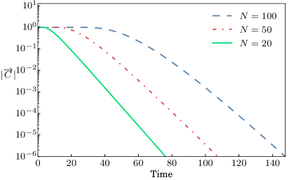
The integral in Eq. 8 depends on $\overrightarrow{C_{t}}(t)=\exp(t\mathbb{J^{(t)}})\overrightarrow{C_{t}}(0)$ which can be written using spectral decomposition as a sum of $N$ terms, each term being associated with one eigenmode and having the time dependence $\exp(t\lambda_{i}^{(t)})$ where $\lambda_{i}^{(t)}$ is the associated eigenvalue. When $N=1$, $\overrightarrow{C_{t}}(t)$ is a constant times a single decaying exponential. Plugging into Eq. 8 then reveals that $T_{t}=\tau_{t}$. The paradox whereby $T_{t}$ can be much larger than $\tau_{t}$ arises only when $N\gg 1$. It is true that each of the $N$ terms contributing to the spectral decomposition of $\overrightarrow{C_{t}}(t)$ decays in magnitude at least as fast as $\exp(-t/\tau)$ but that does not mean that the sum of these terms has that behavior on time scales comparable to $\tau$. Indeed, the terms are not all of the same sign, and their cancellations can lead to long transients before the asymptotic behavior (the exponential decay) prevails. To illustrate this, we show in Fig. 1 the $L_{1}$ norm of $\overrightarrow{C_{t}}(t)$ as a function of $t$ in our toy model consisting of a chain with $a$’s and $b$’s identical across $MA$ reactions. At large times, one sees the exponential decay (a straight line on this semi-log plot) but this asymptotic behavior may set in at times only much longer than $\tau$ itself. The cancellation at short times just mentioned is particularly striking: the curve is very flat for a very long time before it begins to decrease. That waiting time contributes to the large difference between $T_{t}$ and $\tau_{t}$ and is associated with the transient time one must wait for tracer molecules to exit the system.

Figure 2: Leading eigenmode profile for the 20 last metabolites of the chain. Parameters: $a=2$, $b=1$, and $N=20,50,100$.

III.2 Dependence of the characteristic times on $N$

(a)

(b)

Figure 3: Relaxation times(left) and lifetimes(right) for chains between 2 and 100 metabolites long for a perturbation of concentrations and a tracer using the mass action or the Michaelis-Menten-Henri framework. Parameters: $a=2$ and $b=1$, $K_{S}=K_{P}=2$ and $\alpha=aK_{S}$ and $\beta=bK_{P}$ so that the three conditions are comparable. The large $N$ relaxation times are respectively $\tau_{c,\,lim}^{MA}=\tau_{t,\,lim}^{MA}=5.83$, $\tau_{t,\,lim}^{MMH}=11.66$, $\tau_{c,\,lim}^{MMH}=47.66$. The transition sizes between a quadratic and constant or linear behavior are $N_{c,\,cross}^{MA}=N_{t,\,cross}^{MA}=7$, $N_{t,\,cross}^{MMH}=7$, $N_{c,\,cross}^{MMH}=17$.

Assuming the reactions to all have the same parameters and that the steady state is also homogeneous (cf. previous remarks), the relaxation time (be it $\tau_{c}$ or $\tau_{t}$) can be obtained by using the translation invariance of $\mathbb{J^{(c)}}$ and $\mathbb{J^{(t)}}$. Each eigenvector is a product of a sine and an exponential. The formula for the eigenvalues leads to

$$\tau=\frac{1}{A+B-2\sqrt{A\,B}\cos\left(\frac{\pi}{N+1}\right)}$$ (10)

where the quantities $A$ and $B$ are the forward and backward probability of transition per unit of time in the equations linearized about the steady state, entering in $\mathbb{J^{(c)}}$ for $\tau_{c}$ and in $\mathbb{J^{(t)}}$ for $\tau_{t}$. They depend on whether one considers $MA$ or $MMH$ reaction kinetics and whether one considers a concentration perturbation or a tracer, the different cases being enumerated in Table 1.

Parameter	$MA-c$	$MA-t$	$MMH-c$	$MMH-t$
$A$	$a$	$a$	$\frac{\alpha-F}{K_{S}S}$	$\frac{\alpha}{K_{S}S}$
$B$	$b$	$b$	$\frac{\beta+F}{K_{P}S}$	$\frac{\beta}{K_{P}S}$

Table 1: Value of the $A$ and $B$ parameters for the four situations considered. $F$ and $S=(1+c^{ss}/K_{S}+c^{ss}/K_{P})$ are respectively the flux and the saturation factor at steady state in the network for the reactions, the system being by hypothesis homogeneous. The “c” (respectively the “t”) appended to $MA$ and $MMH$ denotes that it is the perturbed concentrations (respectively the tracer concentrations) that are concerned.

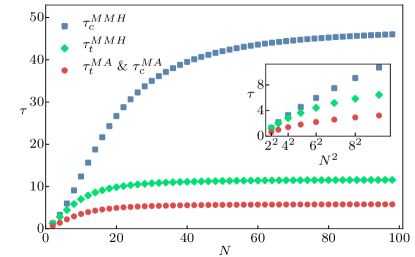
The $\tau$s in the four cases are given by a standardized formula (Eq. 10), it is just that the proper $A$ and $B$ coefficients must be used. Note that for $MA$ kinetics, $\mathbb{J^{(c)}}=\mathbb{J^{(t)}}$ so $\tau_{c}=\tau_{t}$. Furthermore, in both $MA$ and $MMH$ frameworks, when the relative difference between $A$ and $B$ is small, the $\tau$s exhibit two different regimes, one for small chains and one for long chains. For a short chain, $N\ll N^{cross}=\frac{2B\pi}{A-B}$, the characteristic times grow quadratically with the number of metabolites in the chain, a feature characteristic of diffusing systems for the simple reason that if $A=B$, the dynamics is purely diffusive. When $N$ is much above this crossover value, $\tau_{c}$ and $\tau_{t}$ become independent of the chain length as can be seen directly by setting to 1 the cosine in Eq. 10.

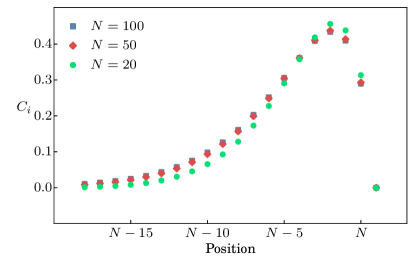
Note that the crossover size $N^{cross}$ diverges as the inverse of $A-B$. Furthermore, in the context of $MMH$ reaction kinetics, this crossover occurs for larger chain lengths when considering the dynamics of a concentration perturbation than when considering tracers because the saturation has the effect of reducing the difference between $A$ and $B$. To illustrate these effects, we display in Fig. 3 the relaxation times as a function of the chain length $N$ for particular values of the kinetic parameters. As for $MA$, $\tau_{c}$ and $\tau_{t}$ do not increase asymptotically with $N$, the characteristic times become independent of the system size. To understand how this occurs, let us examine the leading eigenvector. Its entries depend exponentially on the index $i$ of the node and so its profile is biased towards the largest indices. If the eigenvector with the largest eigenvalue becomes dominant, the major part of the deviation from the steady state is located on a few metabolites (about $N^{cross}$) at the end of the network. As illustrated in Fig. 2, if one increases the number of metabolites, that eigenmode just gets shifted to stay at the same position when measured from the end of the chain. As a consequence, increasing $N$ does not affect the corresponding eigenvalue which determines $\tau$. Thus $\tau_{c}$ and $\tau_{t}$ become independent of $N$ at large $N$.

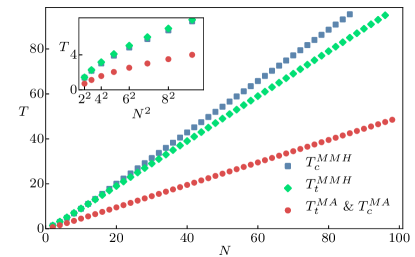
For the $T_{c}$ and $T_{t}$ lifetimes, we did not derive a closed form expression but one can still distinguish between two regimes. If $A-B$ is small the behavior for small $N$ is diffusion-like so $T_{c}$ and $T_{t}$ increases quadratically with $N$. In contrast, for long chains, if $A\neq B$, one has a regime where $T_{c}$ and $T_{t}$ grow linearly with $N$. Similar arguments as for the relaxation times $\tau$ can be invoked to explain these two regimes. In small networks, the diffusion to the two sides of the chain dominates over the mean drift toward one end of the chain. In large networks, assuming $A>B$, most of the transient time dominating $T_{c}$ and $T_{t}$ is dedicated to the transport of the molecules to the $N+1$ end, therefore that transient time is roughly equal to $N$ divided by the drift velocity (which is proportional to $(A-B)$). We illustrate these behaviors in Fig. 3 where one sees again that the various cases behave similarly with the network length. (We already noted that for $MA$ kinetics, $\mathbb{J^{(c)}}=\mathbb{J^{(t)}}$; as a consequence one has $T_{c}=T_{t}$ there, just as one has $\tau_{c}=\tau_{t}$.)

III.3 Effect of the saturation on the characteristic times

The major differences between $MA$ and $MMH$ come from the effect of the saturation. In the case of the $MA$ rate laws, there is no saturation while saturation effects can be important in $MMH$ kinetics. This difference can lead to much larger characteristic time scales in $MMH$ than in $MA$ whenever the concentrations are larger than $K_{S}$ or $K_{P}$. Furthermore, for highly saturated enzymes, the characteristic times can be very different depending on whether one observes a tracer or a perturbation of concentration. Consider a reaction that is near saturation. Introducing a perturbation in the substrate will not change much the flux of that reaction and as a result it will take a long time to dissipate the perturbation away. On the other hand a tracer is essentially unaffected by saturation effects. Indeed, it is not because the reaction is saturated that the tracers cannot participate in the reactions. In effect, the tracers freely pass reactions that are saturated. The main consequence of this phenomenon is that in $MMH$ $\tau_{c}$ can be much larger than $\tau_{t}$ (and $T_{c}$ can be much larger than $T_{t}$).

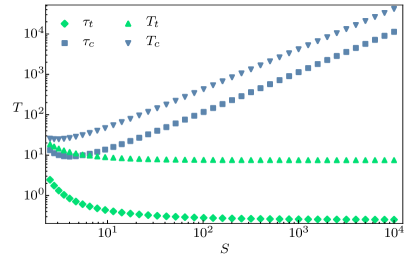
To investigate quantitatively this phenomenon of particular relevance when interpreting kinetic properties from tracer measurements, let us increase saturation effects by reducing $K_{S}$. $K_{P}$ could also have been reduced, but when doing so, the flux in the network may reverse which unnecessarily complicates the analysis. Using the parameters of Table 1 in Eq. 10 for small values of $K_{S}$ gives the following analytical values for the dominant terms of the two relaxation times associated with a tracer ($\tau_{t}$) and with a concentration perturbation ($\tau_{c}$):

$$\tau_{t} \approx \frac{1}{\alpha}$$ (11a)

$$\tau_{c} \approx \frac{\left(\alpha+2\frac{\alpha+\beta}{K_{P}}-2\sqrt{\frac{\alpha}{c}\frac{\alpha+\beta}{K_{P}}\left(1+\frac{\alpha+\beta}{K_{P}}\right)}\cos\left(\frac{\kappa\pi}{N+1}\right)\right)^{-1}}{K_{S}}$$ (11b)

We see from these equations that $\tau_{t}$ is independent of the saturation while $\tau_{c}$ behaves linearly with $1/K_{S}$. Note that the saturation $S=1+c^{ss}/K_{S}+c^{ss}/K_{P}$ scales in the same way for small $K_{S}$. In Fig. 4 we show the dependence of the $\tau$s and the $T$s on the saturation $S$ for both a tracer and a concentration perturbation, assuming $MMH$ rate laws. Not surprisingly, $T_{c}$ is strongly affected by $S$, just as $\tau_{c}$ is.

Figure 4: Relaxation times and lifetimes as a function of the saturation. Parameters: $\alpha=4$, $\beta=2$, $K_{P}=2$, $N=30$. To vary the saturations, the parameter $K_{S}$ is changed over a range going from $1$ to $10^{-4}$.

IV Behavior of characteristic times in more general metabolic networks

IV.1 Effects of disorder in the one dimensional chain

In the disordered (i.e., heterogeneous) case we now consider, the rates “$a$” and “$b$” for the different reactions are taken to be independent random variables. Because every rate is a positive variable, we draw it from a lognormal distribution, i.e., the natural logarithm of a rate $r_{i}$ is distributed according to a Gaussian of mean $\mu$ and standard deviation $\sigma$. Consequently, the mean of $r_{i}$ is $\bar{\mu}=\exp(\mu+\sigma^{2}/2)$ and its variance is $\bar{\sigma}^{2}=(\exp(\sigma^{2})-1)\exp(2\mu+\sigma^{2})$. We impose $\bar{\mu}$ to be equal to the value of the rate in the homogeneous case. An appealing feature of that way of introducing disorder is that the mean drift velocity of a marked molecule in Mass Action remains unchanged, being equal to its disorder average, $\langle a_{i}-b_{i}\rangle$. We are then left with the parameter $\bar{\sigma}$ which can go from 0 to $\infty$ and quantifies the intensity of the disorder. In practice, we use the same coefficient of variation for the “on” and the “off” reaction rates, corresponding to a single measure of intensity of disorder: $CV=\bar{\sigma}_{a}/a=\bar{\sigma}_{b}/b$.

For weak disorder, one expects little change in the values of the characteristic times ($\tau_{c},\tau_{t},T_{c},T_{t}$) compared to the homogeneous case. However, as disorder ($CV$) increases, the characteristic times typically increase. To identify the typical behavior, we have determined these characteristic times for $10,000$ realizations of the disorder and calculated the median times. We illustrate the associated results in Fig. 5 for $\tau_{c}$ and $\tau_{t}$ in the case of Mass Action where those two quantities are equal. Increase is relatively mild (cf. the scales) at low $CV$ butis more marked when $CV$ is larger than $30\%$.

(a)

(b)

Figure 5: Relaxation(left) and transit(right) times as a function of $N$ for several intensities of disorder in the reaction rates as measured by their coefficient of variation $CV$. Main figure: $T=T_{c}=T_{t}$ in the case of Mass Action kinetics. The error bars show the $68.2\%$ confidence interval, value motivated by taking one standard deviation on both sides of the mean of a Gaussian distribution. Parameters: $a=2$, $b=1$, $CV=30\%$ and $70\%$.

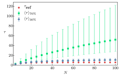
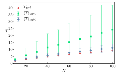
Consider now the effects of disorder on the lifetimes. In Mass Action, $T_{c}=T_{t}$, even in the presence of disorder. We display in Fig. 5 the dependence of these quantities on $N$ for several values of $CV$ and see that disorder has little effect as long as $CV$ is small. This can be justified by noticing that the drift velocity of a molecule at site $i$ is $a_{i}-b_{i-1}$ and its ensemble average (as in an annealed approximation) is the same as without disorder, namely $a-b$. At large disorder this argument fails because the quenched and annealed averages are very different. An extreme case can be seen from the fact that a large value of “$a$” at one site cannot compensate a small value at another site. At large $CV$, one sees clear effects of disorder. The reason should be clear: $T_{c}$ and $T_{t}$ are sensitive to unfavorable reactions (for instance where $a$ is small) throughout the whole chain of reactions.

IV.2 Networks with branches and loops

Although quite a few biosynthetic pathways include successive steps forming a chain of enzymatic reactions, the one dimensional systems considered so far remain toy models because in all known organisms, large scale biochemical metabolic networks have numerous branches and loops. It is thus necessary to consider how characteristic time scales might be affected by such structures. Rather than produce artificial networks including those features, it is more relevant to study directly the various kinetic models of metabolism that have been proposed in the literature. The repository “Biomodels” Le Novère et al. (2006); Hucka et al. (2003) provides the gold standards for such models both because the models must past tests to be deposited and because their availability ensures that they can be compared to state of the art. Focusing further on those models that have been manually curated, we are left with only a handful of cases. The reason is that measuring kinetic constants of enzymes is a very difficult task so almost always when building a kinetic model the modeler has to use indirect methods to overcome the problem of dealing with many unknown parameters. We studied four of these models, published respectively in Teusink et al. (2000); Chassagnole et al. (2002); Mosca et al. (2012); Curto et al. (1998).

For each of those four kinetic models, we first downloaded its SBML specification Hucka et al. (2003) from the repository and exported the ordinary differential equations into Python code that can be processed. Once in our format, we determined the steady state of the network of reactions and we then computed the matrices $\mathbb{J^{(c)}}$ and $\mathbb{J^{(t)}}$. The associated leading eigenvectors and eigenvalues were obtained using the inverse power method, thereby providing the values of $\tau_{c}$ and $\tau_{t}$. Furthermore numerical integration was used to compute $T_{c}$ and $T_{t}$ according to Eqs. 8and 9. The initial perturbation was taken to be localized at the first metabolite produced from the compound entering the network from the outside reservoir.

In Table 2 we provide the values of the four characteristic times for each of the Biomodels studied. The first model Teusink et al. (2000) contains the reactions for glycolysis in S. cerevisiae (baker’s yeast). It has 17 reactions, mostly of the reversible $MMH$ type, and there are 14 internal metabolites. Glucose is an external metabolite which enters the metabolism and then gets transformed. A total of 3 compounds can be excreted, all irreversibly. The characteristic times of this model are short, from a few seconds to a few minutes. Further inspection shows that the ordering of these four values follows the same pattern as in our one dimensional toy model, namely

$$\tau_{t}<\tau_{c}<T_{t}<T_{c}$$ (12)

This can be justified as follows. First, $\tau_{t}>\tau_{c}$ and $T_{t}>T_{c}$ because a labeled atom is not subject to Michelis-Menten saturation effects. The saturation of flux in a reaction may prevent a concentration fluctuation from being evacuated but it will not prevent labeled atoms from going through (participating to the flux). Furthermore, in our toy model, the $\tau$s are relatively insensitive to processes inside the network, they depend mainly on reactions close to the excreted metabolites, while the $T$s depend on drift throughout the whole network and thus should be larger than the $\tau$s.

The other models follow quite closely this same pattern (cf. Table 2). Model 2 contains the reactions for the glycolysis and the pentose phosphate pathway in E. coli Chassagnole et al. (2002). It has 48 reactions and 17 internal metabolites, but we needed to remove the model’s explicit time dependence to obtain a meaningful steady state. The main difference with the model 1 is the modelled organism and the glucose steady state uptake rate ($3.1\leavevmode\nobreak\ \mu mol.s^{-1}.L^{-1}$ compared to $1.5\leavevmode\nobreak\ mmol.s^{-1}.L^{-1}$) but Eq. 12 is respected. Again model 3 contains the glycolysis and the pentose phosphate pathway, but for a human cancer cell. It has 29 reactions and 34 internal metabolites. The glucose uptake, expressed per gram of cell dry weight ($0.17mmol.s^{-1}.gcdw^{-1}$), cannot be compared to the two previous uptakes but Eq. 12 is mostly verified.

Model 4 contains the reactions for the biosynthesis of purines in E. coli Curto et al. (1998). It has a total of 29 reactions and 18 internal metabolites. The main difference compared to the other three models is that the formalism uses kinetics that are neither $MA$ nor $MMH$: the forward and backward rates of the reactions are fractional powers of the concentrations of the metabolites. Such fractional powers are often used phenomenologically to parametrize allosteric or regulatory effects; they have the drawback that the flux may rise very steeply when starting with low concentrations; although this may be the case for some regulatory processes, it can lead to a situation where a concentration perturbation will be evacuated more efficiently than a labeled atom. Such a possibility seems to be realized in this model as in Table 2 one sees that $\tau_{c}<\tau_{t}$ and $T_{c}<T_{t}$.

time (s)	$\tau_{c}$	$\tau_{t}$	$T_{c}$	$T_{t}$
Model 1 Teusink et al. (2000)	$15.$	$3.75$	$339$	$84.4$
Model 2 Chassagnole et al. (2002)	$120$	$95.2$	$2834$	$2210$
Model 3 Mosca et al. (2012)	4.94	0.16	107	3.53
Model 4 Curto et al. (1998)	$4.34\leavevmode\nobreak\ 10^{5}$	$1.11\leavevmode\nobreak\ 10^{6}$	$9.35\leavevmode\nobreak\ 10^{6}$	$2.36\leavevmode\nobreak\ 10^{7}$

Table 2: Value of the characteristic times $\tau_{c}$, $\tau_{t}$, $T_{c}$ and $T_{t}$ in seconds for the four manually curated models Curto et al. (1998); Teusink et al. (2000); Chassagnole et al. (2002); Mosca et al. (2012) we have studied and that are available on the Biomodels repository Le Novère et al. (2006).

V Discussion and conclusions

The damping of a concentration fluctuation generally requires the perturbation to spread out but in our reaction network the drift plays a central role. The time scale for evacuating a perturbation is what we call its lifetime $T$ (cf. Eqs. 8 and  9), though in other contexts it can be referred to as the mean residence or transit time. In the absence of a drift, corresponding to a pure diffusive regime, the lifetime $T$ scales as the square of the diameter of the network, a scaling which also arises for the standard measure of return to equilibrium via the relaxation time $\tau$. That is the situation one is most familiar with, and there $\tau$ provides the longest characteristic time as it should. However, for typical reaction networks, one has both diffusion and drift. In particular, out of equilibrium systems will have fluxes, and such fluxes may drive labeled atoms out of the network just as drift does. In the presence of such drift, a perturbation’s lifetime $T$ can scale as the diameter of the network divided by a characteristic drift velocity which is related to the presence of flux. Interestingly, in this out of equilibrium situation, the relaxation time $\tau$ is no longer informative about the time scale of the (slow) process which evacuates perturbations. In particular, in our toy model consisting of a homogeneous chain of reactions, $\tau$ did not grow with the system size while $T$ grew linearly. We showed analytically how that could be in that system, but the phenomenon is general. Indeed, in the presence of drift, the linearized dynamics can be decomposed into eigenvectors, but the leading eigenvector determining $\tau$ tends to be concentrated on the metabolites that can be excreted. As a result, $\tau$ is quite insensitive to the size of the network while $T$ inevitably increases with network size since the evacuation of a perturbation requires it to cross the diameter of the network. These phenomena are most easily understood when the reactions obey mass action, but they arise also for Michaelis-Menten-Henri reaction laws. For this last case, the existence of a saturation of the flux with concentration of metabolites exacerbates the difference between $T$ and $\tau$. Interestingly, the dynamics of labeled atoms that are often used to investigate kinetic properties of networks are far less sensitive to these saturation effects. As a consequence, the use of isotopic labelings can lead to severely underestimate the longest characteristic time in these reaction networks.