Assortativity and leadership emerge from anti-preferential attachment in heterogeneous networks

Abstract

Real-world networks have distinct topologies, with marked deviations from purely random networks. Many real-world networks exhibit degree-assortativity, with nodes of similar degree more likely to link to one another. Though microscopic mechanisms have been suggested for the emergence of other topological features, assortativity has proven elusive. Though assortativity can be artificially implanted in a network via degree-preserving link permutations, this destroys the graph’s hierarchical clustering and does not correspond to any microscopic mechanism. Here, we propose the first generative model which creates heterogeneous networks with scale-free-like properties in degree and clustering distributions and tunable realistic assortativity. Two distinct populations of nodes are incrementally added to an initial network by selecting a subgraph to connect to at random. One population (the followers) follows preferential attachment, while the other population (the potential leaders) connects via anti-preferential attachment: they link to lower degree nodes when added to the network. By selecting the lower degree nodes, the potential leader nodes maintain high visibility during the growth process, eventually growing into hubs. The evolution of links in Facebook empirically validates the connection between the initial anti-preferential attachment and long term high degree. In this way, our work sheds new light on the structure and evolution of social networks.

Introduction

Networks with scale-free(SF)-like degree distributions represent a wide range of systemsAlbert et al. (2000); Albert and Barabási (2002); Wuchty et al. (2003); Newman (2003a); Boccaletti et al. (2006, 2014). The topology of real-world networks (RWNs) often features deviations from a pure power-law distributionAlbert and Barabási (2002) $P_{k}\sim k^{-\gamma}$, together with hierarchical clusteringRavasz et al. (2002) $C_{k}\sim k^{-\omega}$. One ubiquitous feature of many RWNs is degree-degree correlations: two nodes are more likely to be linked to one another if they are of similar (assortative) or dissimilar (disassortative) degree. Assortativity is generally found in social and collaboration RWNs, while disassortativity is common in technological and biological RWNsNewman (2002, 2003b).

SF networks have been studied in the context of generative models, and simple rules relating to the formation of new links have been shown to lead to power-law degree distributions with non-hierarchicalBoccaletti et al. (2007); Brede (2011) and hierarchicalBarabási and Albert (1999); Dorogovtsev et al. (2000); Vázquez (2003); Chung et al. (2003); Krapivsky and Redner (2005); Clauset et al. (2008); Lorimer et al. (2015) traits. Static SF network modelsBender and Canfield (1978) have also been proposed with controlled assortativityZhou et al. (2008); Bassler et al. (2015), and growing SF networks have been studied with assortativeCatanzaro et al. (2004); Quayle et al. (2006); Toivonen et al. (2006); Nguyen and Tran (2010); Shang (2014), disassortativeBoccaletti et al. (2007); Šubelj and Bajec (2013) and both typesBrede (2011) of degree mixing.

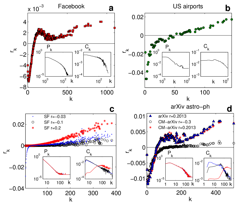
In particular, a wide range of RWNs feature assortativityKunegis (2013), including online socialViswanath et al. (2009), and neuralTeller et al. (2014); de Santos-Sierra et al. (2014) networks. As it reflects a basic birds of a feather flock together property, it is not surprising that it is so ubiquitous. Rather, what is really surprising is that the contributions of different nodes to the graph assortativity level $r$ strongly depend on the degree. Decomposing the assortativity spectrum, one can indeed describe the local assortativity or assortativenessPiraveenan et al. (2008) $r_{k}$ of each set of nodes with a given degree $k$ (see the Methods section). Many RWNs have a pronounced local maximum in $r_{k}$ located near (but above) the average degree $\langle k\rangle$. In social networks such a feature even appears to be generic, while in technological and biological networks the maximum is less pronounced or even entirely absent. In Fig. 1 we show the qualitative difference in the inherent patterns of $r_{k}$ between typical social networks (the friendship structure of Facebook usersViswanath et al. (2009) and the Authors’ collaboration graph from the arXiv’s Astrophysics sectionLeskovec et al. (2007); Whitfield (2008); Eom and Jo (2014)) and a technological one (the flights connecting the 500 busiest commercial airports in the United StatesColizza et al. (2007)).

Figure 1: Local assortativity $r_{k}$ vs. the node degree $k$ for realKunegis (2013) and artificial networks. (a) Data from friendships of Facebook usersViswanath et al. (2009) ($N=63,392$, $L=816,886$, $\langle k\rangle=26$, $r=0.1768$). (b) Network of the 500 busiest commercial airports in the United StatesColizza et al. (2007). A tie exists between two airports if a flight was scheduled in 2002. ($N=500$, $L=2,980$, $\langle k\rangle=11.92$, $r=-0.2678$). (c) Random SF networks ($N=10,000$, $\langle k\rangle=10$) with almost neutral ($r=-0.03$, blue dots), disassortative ($r=-0.1$, black circles) and assortative ($r=0.2$, red stars) mixing. (d) The Authors’ collaboration graph from the arXiv’s Astrophysics sectionLeskovec et al. (2007) ($N=17,903$, $L=196,972$, $\langle k\rangle=22$, $r=0.2013$). Together with the real data (blue triangles), $r_{k}$ is reported for a CM reproducing the real degree sequence, after classical permutation methods have been applied, imposing the same $r$ value observed in the real network (red stars) and a negative ($r=-0.3$) value (black circles). Insets in panels (a-d) show the log-log plots of the degree distributions $P_{k}$ and clustering coefficient $C_{k}$.

Results

Empirical observations.

The way traditional methods imprint assortativity into pre-generated networks is via degree-preserving link permutationsNewman (2003b); Xulvi-Brunet and Sokolov (2004). This approach yet presents a number of problems. On the one hand, generating a graph with an ad-hoc imprinted SF distribution (Fig. 1c) and then rewiring connections does not yield the observed pattern of local assortativity, on the other hand, even starting from a configuration model (CM) retaining the original degree distributionBender and Canfield (1978), this procedure is only able to reproduce the real assortativity pattern at the expense of destroying the other significant features, such as the hierarchical inherent structure of clustering (Fig. 1d and its bottom-right inset). This indicates that the systemic mechanisms leading to the emergence of degree-correlation have a special signature, which is not captured when generating assortativity artificially, i.e., ex post facto.

Further striking evidence comes to light from a deeper analysis of social RWNs: in some cases the final leaders (i.e. the nodes that, at the end of the process, do acquire a leading role in terms of their degree) actually behave anti-preferentially when entering the network. In Fig. 2, the Facebook network of Fig. 1a is examined, and one sees that, plotting the degree of the first linked node as a function of time, those nodes eventually becoming the network’s leaders (i.e. the final hubs, red triangles) tend initially (at the moment at which they start forming part of the network) to link existing nodes with low degree values (Fig. 2a). This is clearer from Fig. 2b where the final degree $k_{f}$ achieved by a given node, labeled as a red triangle ($k_{f}>400$), a black square ($40<k_{f}<400$) or a blue circle ($k_{f}<40$), is compared to the degree of its first neighbor at the time that node entered the network. A straightforward statistical analysis of the data shows in Fig. 2c that indeed the fraction of final hubs forming initial connections with nodes of low-medium degrees is far larger than that of the nodes which ultimately acquire intermediate and low degrees.

Figure 2: Nodes’ selection mechanisms of their initial neighbors in RWNs. The Facebook network analyzed in Fig. 1a. (a) Degree of the nodes chosen as first connections by those nodes whose final (i.e. at the end of the growth process) degree $k_{f}$ is low ($k_{f}<40$, blue circles), high ($k_{f}>400$, red triangles), and intermediate ($40\leq k_{f}\leq 400$, black squares). The reported values are from the largest connected component of the Facebook network of Fig. 1a formed only by those edges that are time-stamped ($N=60,663$, $L=614,541$, $\langle k\rangle=20$, $r=0.1851$). (b) Log-linear plot of of the final degree $k_{f}$ of each node (labeled according to the legend in Fig. 2c) as a function of the degree of its first connection. (c) Log-linear plot of the fraction of high (red triangles), medium (black squares) and low (blue circles) degree nodes establishing their first link with a node of a given degree.

The generative model.

Following the empircal observation in Fig. 2 of a nexus between initial anti-preferential attachments and long-term high degrees, we propose a generative model which creates SF-like networks with tunable global assortativity and realistic local assortativity patterns, while also reproducing the hierarchical structure of the network’s clustering. The model reflects a microscopic mechanism for a struggle for leadership between two competing populations of nodes: type I nodes (acting as followers and selecting connections so that a preferential attachment rule spontaneously emergesBoccaletti et al. (2007)) and type II nodes (acting as potential leaders, i.e. adopting anti-preferential behavior which leads them to prefer lower degree nodes for the establishment of their initial links).

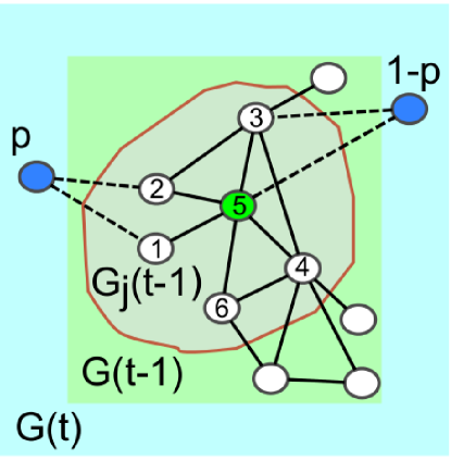
Under such a mechanism, a network of $N$ nodes is created by sequentially adding units to an initial clique of $m\leq N_{0}\lll N$ vertices. The growing process occurs at discrete times: at each time step $1\leq t\leq N-N_{0}$ a new node enters the graph, and forms $m$ links with existing nodes according to an attachment rule that is illustrated schematically in Fig. 3 and summarized as follows:

1. An anchor node $j$ is selected uniformly at random from the nodes existing at time $t-1$.

2. The subgraph $G_{j}$ composed of node $j$ and all other nodes that are at distance less than or equal to $\ell$ from $j$ is examined.

3. With probability $1-p$, the new node behaves as a follower (type I): it selects $m$ nodes from $G_{j}$ uniformly at random, and links to them. With probability $p$, the new node behaves instead as a potential leader (type II): it forms links with the $m$ lowest degree nodes in $G_{j}$.

The parameter $\ell$ is defined as the so called penetration depth, i.e. the extent of local information (around the anchor $j$) accessible to the entering node. In the following, we set $\ell=1$, so that ${G}_{j}$ is the subgraph containing $j$ and all its nearest neighbors. Once $\ell=1$ is set, the model is uniquely determined by two parameters: the average degree $\langle k\rangle=2m$ and $p$, the fraction of type II nodes. In the absence of potential leaders ($p=0$), the growth of the resulting network exhibits emergent preferential attachment and hierarchical clusteringBoccaletti et al. (2007): the $p=0$ case produces a pure SF network with degree distribution Albert and Barabási (2002); Newman (2003a) $P_{k}\sim k^{-3}$, and with additional hierarchical SF clusteringRavasz et al. (2002) $C_{k}\sim k^{-1}$. This is actually due to the so called friendship paradoxFeld (1991), stating that, averaged across the network, the neighbors of a node $i$ will always have a higher average degree than $k_{i}$. Since, indeed, the number of subgraphs $G_{j}$ in which a node $i$ appears is equal to $k_{i}+1$, higher degree nodes will tend to naturally receive more and more links. It is important to note that this preferential behavior is in fact, emergent: the entering nodes do not require global knowledge of the degree levels in the system, nor any explicit preference for high degree nodes. In that sense, preferential attachment can be viewed as a kind of null behavior in which the rate of growth increases with size, as the analogous Yule process is understood in evolutionary dynamicsYule (1925); Simon (1955).

Figure 3: The network growth process. At time $t$, the graph $G(t)$ is updated with a new node (blue circle) which forms $m$ connections (in the example $m=2$, dashed lines) within the subgraph $G_{j}(t-1)$ with a probability $p$ to the lowest degree nodes (nodes 1 and 2) or with probability $1-p$ at random (nodes 3 and 5). The subgraph $G_{j}(t-1)$ is composed of a randomly chosen node $j$ (node 5, green circle) and its nearest neighbors at time $t-1$.

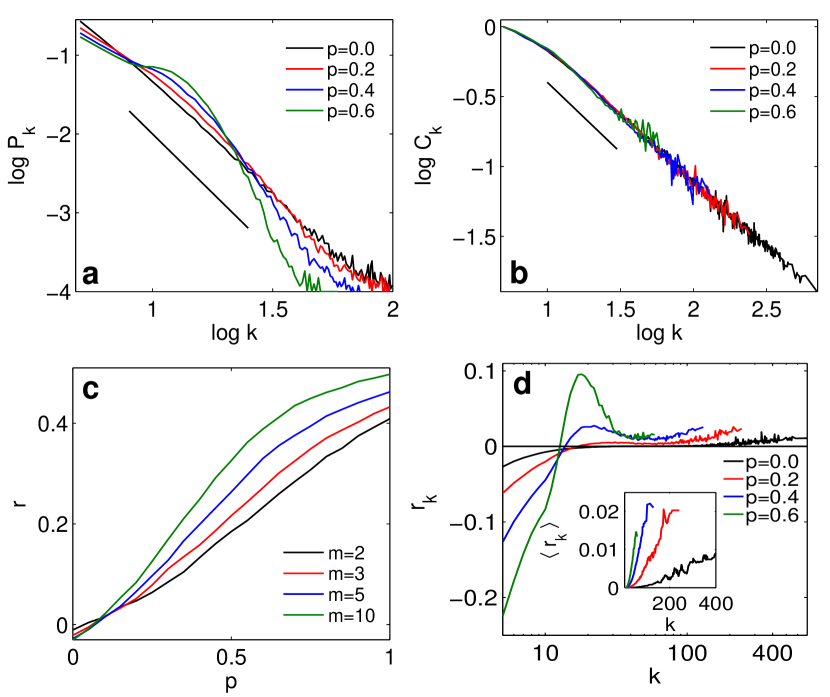
When instead the population is split (with some nodes following the null preferential attachment, and some others linking in an anti-preferential manner), the local assortativity pattern shown in Fig. 1a, characterizing social systems, emerges. Namely, the contribution to assortativity from nodes of degree $k$ i) increases with $k$ from $k=1$ to a local maximum located just above the average degree, ii) decreases to a subsequent local minimum, and then iii) increases again as $k\rightarrow\infty$, i.e. qualitatively reproducing the generic tendency observed in social RWNs, which is only captured in random generated networks with artificially induced assortativity at the expense of obliterating the graph’s clustering traits. The results of the model are summarized in Fig. 4. As $p$ increases, the degree distribution of the resulting network deviates more and more from a pure SF configuration (Fig. 4a), but at the same time the hierarchical clustering traits are entirely preserved (Fig. 4b). The generated network is actually endowed with a fully controllable and tunable level of global assortativity $r$ (as a function of $m$, as shown in Fig. 4c), while, more remarkably, the assortativity local pattern is fully reproduced (Fig. 4d).

Analytical description.

We next move toward giving a more analytic description of the motivations and roots underlying the proposed model and the observed, emergent phenomena. We start by noting that links in this model are undirected, and this leads to a symmetry of interpretations: one can describe the type II nodes as preferring low-degree units (as it is described in our generative model), or one can state that low-degree nodes are more likely to create links with type II newcomers. The second interpretation is actually in line with what arises from recent sociological studies, which indeed indicate that people are limited in the number of relationships they can maintain over time (with the exact number of maximal relationships being an open question). Starting from the seminal works by DunbarDunbar (1992); Hill and Dunbar (2003), the limitations on the number of active social connections have been extensively studied and empirical support from online social networks has also been adducedGonçalves et al. (2011). In the present case, the emergence of positive assortativity is associated with the interplay of two mechanisms: an innate preferential attachment (resulting from nodes that nonhierarchically form connections with a pre-existing growing structure) and a limited ability of human beings to maintain many relationships.

By comparing the average contribution of assortativity per node of degree $k$, $\langle r_{k}\rangle$, and the total contribution of nodes of degree $k$, $r_{k}$, one can actually understand the origin of the peak in the local assortativity. The average contribution for nodes of degree $k$ increases monotonically with $k$ (inset of Fig. 4d). However, the frequency of nodes decreases monotonically with $k$ in pure scale-free networks (Fig. 4a). With the introduction of type II nodes, lower-medium degree nodes become more frequent, as observed in Fig. 4a for $p=0.6$, even though an overall scale-free-like degree distribution is maintained. The combination of more-common than expected medium degree nodes and per-node contribution to assortativity that increases with $k$ leads to the characteristic bump observed in the model and the data.

As the network’s growth proceeds, type II nodes actually tend to develop a higher degree on average. This is because new links are obtained with probability

$$P\sim\frac{1}{N_{t}}\frac{m}{|G_{j}|}$$ (1)

where $N_{t}$ is the number of nodes in the system at time $t$ and $|G_{j}|$ is the size of the neighborhood of the subgraph of a given anchor node $j$. By choosing anchor nodes with small $|G_{j}|$ (low degree), type II nodes actually increase their likelihood of being linked from future, incoming, nodes. Because this increased likelihood can be understood as type II nodes “placing themselves” in smaller neighborhoods so that they are more likely to be linked to than when chosen at random, we understand this advantage as a kind of improved visibility to the linking process.

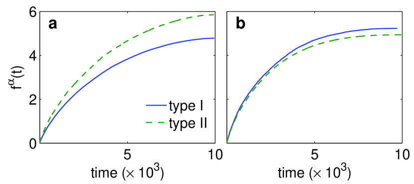
In fact, one can measure the number of neighbors at time $t$ for each node type as described in the Methods section. The results are shown in Fig. 5, and point to the emergence of leadership of type II nodes at low values of $p$ (Fig. 5a). At intermediate values of $p$ (not shown) no significant differences are observed between the two nodes’ populations in the way the average increased degree evolves in time. Only at large $p$ values (Fig. 5b), where anti-preferential nodes are vastly predominant in number the trend is actually reversed and type I nodes (the followers) now seem to be favored in attracting connections. Such a latter situation corresponds however to a rather homogeneous network, where a SF-like distribution is no longer observed (see Fig. 4 for comparing the large deviations in the degree distribution already observed at $p=0.6$).

Discussion

In summary, assortativity, hierarchical structure and fat-tailed degree distributions (well-approximated by power laws) are structural features manifested almost ubiquitously by RWNs, and until now no model had linked their emergence with microscopic growing assumptions. Furthermore, these features have a fundamental role in determining many relevant processes, and/or regulating the network’s dynamics and functioning. Guided by the empirical observation of the growth of the friendship network of Facebook users, we have shown how the combination of preferential and anti-preferential attachment mechanisms acting together in the same generative model (via two distinct node populations), leads to the growth of heterogeneous networks with modified scale-free properties and tunable realistic assortativity, while maintaining the hierarchical clustering. Both our analytical predictions and numerical results indicate that networks constructed in this way match the patterns of local assortativity measured in real-world graphs. By presenting the first generative model with tunable assortativity, this work sheds new light on the structure and evolution of social networks, and counterintuitively suggests that anti-preferential attachment is a mechanism adopted by a fraction of the nodes during the network’s growth, as a strategy for increasing their own leadership.

Figure 4: Emergent topology in the generated network. (a) Normalized degree distribution $P_{k}$ (log₁₀ scale) vs. the logarithm (base 10) of $k$, and (b) $\log_{10}-\log_{10}$ plot of $C_{k}$ vs. $k$, for $m=5$ and different values of the probability $p$ (see legend for color-coding). (c) Assortativity coefficient $r$ vs. $p$, for different values of $m$ (see legend for color-coding). (d) Log-linear plot of the local assortativity $r_{k}$ (main panel) and average local assortativity $\langle r_{k}\rangle$ (inset) vs. $k$, for $m=5$ and several values of $p$ (see legend for color-coding). In all cases, $N=10^{4}$, $N_{0}=10$, and each point refers to an ensemble average over 20 network realizations. As a guide for the eyes, the straight lines in (a) and (b) stay for the functions $P_{k}\propto k^{-3}$ and $C_{k}\propto k^{-1}$, respectively.

Figure 5: Emergence of leadership during the growth process. Average increased degree (the degree acquired after nodes have first appeared in the graph, vertical axes) as a function of time (horizontal axis), for type I (followers) and type II (potential leaders) nodes, and for (a) $p=0.2$, and (b) $p=0.8$. See the Methods section for the explanation on how the reported values are calculated. Panels report the average increased degree $f^{\alpha}(t)$ of the nodes of different types ($\alpha=$type I or II), after having been in the system for $t$ steps. $N=10^{4}$, $N_{0}=5$ and $m=5$. Color and line style codes are defined in the legend of panel (a).

Methods

Local assortativity/assortativeness.

In a network with $N$ nodes, $L$ links and degree distribution $P_{k}$, the local assortativity or assortativeness Piraveenan et al. (2008) $r_{j}$ is defined as the contribution of each node to the network assortativity $r$ and it is calculated as

$$r_{j}={(\alpha_{j}-\beta_{j})}/{\sigma_{q}^{2}},$$

with $r_{k}=\sum_{j|k_{j}=k}r_{j}$ being the total of the local assortativity values of nodes with a given degree $k$ such that $r=\sum_{k}r_{k}$. In the above expression, $\alpha_{j}=\frac{\hat{k}_{j}}{2L}\sum_{i=1}^{k_{j}}\hat{k}_{i},$ and $\beta_{j}=k_{j}\frac{\mu_{q}^{2}}{2L}$, being $\hat{k}_{j}=k_{j}-1$ the remaining degree of node $j$, $\hat{k}_{i}$ the remaining degrees $\hat{k}_{1},\hat{k}_{2},\dots,\hat{k}_{k_{j}}$ of the $k_{j}$ nodes connected to node $j$, and $\mu_{q}$ and $\sigma_{q}$ the first and second moments of the remaining degree distribution $q_{k}=\frac{(k+1)P_{k+1}}{\sum_{j}jP_{j}}$.

Measuring the average degree of each node type.

In order to compare the average degree of the two node populations as the model evolves, we label each node uniquely by the step in which it entered the network. This way, at time $t$, every node $i$ will have $m$ neighbors with indices $j<i$, and $k_{i}(t)-m$ neighbors with indices $j>i$. To compare the degree growth rates of type I and type II nodes, we need to measure the characteristic time for new links to form. To do so, we consider the set of differences in index values, $j-i$, for each neighbor which linked to $i$ at step $j$

$$\tau_{i}^{\alpha}=\{(j-i)\,\,|\,\,{\text{with}}j\in{\cal N}_{i}\land(j>i)\},$$ (2)

with $\alpha=I,II$ designating the node type and ${\cal N}_{i}\land(j>i)$ the neighborhood of $i$. Combining these sets for all nodes of each type, one obtains the non-unique set

$$\tau^{\alpha}=\mathop{\cup}_{i=1}\tau_{i}^{\alpha}.$$ (3)

Using Eq. (3), one can measure the expected number of neighbors (after $t$ steps) for each node type via

$$f^{\alpha}(t)=\frac{1}{N^{\alpha}}\lvert\{i\,\,|\,\,i\in\tau^{\alpha}\land i<t\}\rvert,$$ (4)

where $N^{\alpha}$ is the total number of nodes of type $\alpha$. Thus $f^{\alpha}(t)$ provides the average number of new neighbors ($\langle k\rangle-m$) that a node of type $\alpha$ will acquire after $t$ steps.

References

- Albert et al. (2000) R. Albert, H. Jeong, and A.-L. Barabasi, Nature 406, 378 (2000).
- Albert and Barabási (2002) R. Albert and A.-L. Barabási, Rev. Mod. Phys 74, 47 (2002).
- Wuchty et al. (2003) S. Wuchty, Z. N. Oltvai, and A.-L. Barabasi, Nat. Genet. 35, 176 (2003).
- Newman (2003a) M. E. J. Newman, SIAM Review 45, 167 (2003a).
- Boccaletti et al. (2006) S. Boccaletti, V. Latora, Y. Moreno, M. Chavez, and D. Hwang, Phys. Rep. 424, 175 (2006).
- Boccaletti et al. (2014) S. Boccaletti, G. Bianconi, R. Criado, C. I. del Genio, J. Gómez-Gardeñes, M. Romance, I. Sendiña-Nadal, Z. Wang, and M. Zanin, Phys. Rep. 544, 1 (2014).
- Ravasz et al. (2002) E. Ravasz, A. L. Somera, D. A. Mongru, Z. N. Oltvai, and A. L. Barabási, Science 297, 1551 (2002).
- Newman (2002) M. Newman, Phys. Rev. Lett. 89, 208701 (2002).
- Newman (2003b) M. Newman, Phys. Rev. E 67, 026126 (2003b).
- Boccaletti et al. (2007) S. Boccaletti, D.-U. Hwang, and V. Latora, IJBC 17, 2447 (2007).
- Brede (2011) M. Brede, Artificial Life 17, 281 (2011).
- Barabási and Albert (1999) A.-L. Barabási and R. a. Albert, Science 286, 509 (1999).
- Dorogovtsev et al. (2000) S. N. Dorogovtsev, J. F. Mendes, and a. N. Samukhin, Phys. Rev. Lett. 85, 4633 (2000).
- Vázquez (2003) A. Vázquez, Phys. Rev. E 67, 056104 (2003).
- Chung et al. (2003) F. Chung, L. Lu, T. G. Dewey, and D. J. Galas, J. Comp. Biol. , 677 (2003).
- Krapivsky and Redner (2005) P. L. Krapivsky and S. Redner, Phys. Rev. E 71, 036118 (2005).
- Clauset et al. (2008) A. Clauset, C. Moore, and M. E. J. Newman, Nature 453, 98 (2008).
- Lorimer et al. (2015) T. Lorimer, F. Gomez, and R. Stoop, Sci. Rep. 5, 12353 (2015).
- Bender and Canfield (1978) E. A. Bender and E. Canfield, Journal of Combinatorial Theory, Series A 24, 296 (1978).
- Zhou et al. (2008) J. Zhou, X. Xu, J. Zhang, J. Sun, M. Small, and J.-a. Lu, IJBC 18, 3495 (2008).
- Bassler et al. (2015) K. E. Bassler, C. I. D. Genio, P. L. Erdös, I. Miklós, and Z. Toroczkai, New J. Phys. 17, 083052 (2015).
- Catanzaro et al. (2004) M. Catanzaro, G. Caldarelli, and L. Pietronero, Physica A 338, 119 (2004).
- Quayle et al. (2006) A. Quayle, A. Siddiqui, and S. J. Jones, EPJ B 50, 617 (2006).
- Toivonen et al. (2006) R. Toivonen, J.-P. Onnela, J. Saramäki, J. Hyvönen, and K. Kaski, Physica A 371, 851 (2006).
- Nguyen and Tran (2010) K. Nguyen and D. Tran, in Communications and Electronics (ICCE) (2010) pp. 30–35.
- Shang (2014) Y. Shang, The Scientific World Journal 2014, 759391 (2014).
- Šubelj and Bajec (2013) L. Šubelj and M. Bajec, in 22Nd International Conference on WWW Companion (2013) pp. 527–530.
- Kunegis (2013) J. Kunegis, in Int. Web Observatory Workshop (2013) pp. 1343–1350.
- Viswanath et al. (2009) B. Viswanath, A. Mislove, M. Cha, and K. P. Gummadi, in 2nd ACM Workshop on Online Social Networks, WOSN ’09 (ACM, 2009) pp. 37–42.
- Teller et al. (2014) S. Teller, C. Granell, M. De Domenico, J. Soriano, S. Gomez, and A. Arenas, PLoS Comput. Biol. 10, e1003796 (2014).
- de Santos-Sierra et al. (2014) D. de Santos-Sierra, I. Sendiña Nadal, I. Leyva, J. a. Almendral, S. Anava, A. Ayali, D. Papo, and S. Boccaletti, PLoS ONE 9, e85828 (2014).
- Piraveenan et al. (2008) M. Piraveenan, M. Prokopenko, and a. Y. Zomaya, EPL 84, 28002 (2008).
- Leskovec et al. (2007) J. Leskovec, J. Kleinberg, and C. Faloutsos, ACM Trans. Knowledge Discovery from Data 1, 1 (2007).
- Whitfield (2008) J. Whitfield, Nature 455, 720 (2008).
- Eom and Jo (2014) Y.-H. Eom and H.-H. Jo, Sci. Rep. 4, 4603 (2014).
- Colizza et al. (2007) V. Colizza, R. Pastor-Satorras, and A. Vespignani, Nat. Phys. 3, 276 (2007).
- Xulvi-Brunet and Sokolov (2004) R. Xulvi-Brunet and I. Sokolov, Phys. Rev. E 70, 066102 (2004).
- Feld (1991) S. L. Feld, American Journal of Sociology 96, 1464 (1991).
- Yule (1925) G. U. Yule, Phil. Trans. R. Soc. B 213, 21 (1925).
- Simon (1955) H. A. Simon, Biometrika 42, 425 (1955).
- Dunbar (1992) R. I. Dunbar, Journal of Human Evolution 22, 469 (1992).
- Hill and Dunbar (2003) R. Hill and R. Dunbar, Human Nature 14, 53 (2003).
- Gonçalves et al. (2011) B. Gonçalves, N. Perra, and A. Vespignani, PLoS ONE 6, e22656 (2011).