Sufficient and necessary conditions for Dynamic Programming in Valuation-Based Systems.

Abstract

Valuation algebras abstract a large number of formalisms for automated reasoning and enable the definition of generic inference procedures. Many of these formalisms provide some notion of solution. Typical examples are satisfying assignments in constraint systems, models in logics or solutions to linear equation systems.

Many widely used dynamic programming algorithms for optimization problems rely on low treewidth decompositions and can be understood as particular cases of a single algorithmic scheme for finding solutions in a valuation algebra. The most encompassing description of this algorithmic scheme to date has been proposed by Pouly and Kohlas together with sufficient conditions for its correctness. Unfortunately, the formalization relies on a theorem for which we provide counterexamples. In spite of that, the mainline of Pouly and Kohlas’ theory is correct, although some of the necessary conditions have to be revised. In this paper we analyze the impact that the counter-examples have on the theory, and rebuild the theory providing correct sufficient conditions for the algorithms. Furthermore, we also provide necessary conditions for the algorithms, allowing for a sharper characterization of when the algorithmic scheme can be applied.

1 Introduction

Solving optimization problems is an important and well-studied task in computer science. There are many optimization problems whose solution can be expressed as an assignment of values to a set of variables. Usually, the larger the number of variables involved in the problem, the more complex it is to find a solution. A particular approach to tackle problems whose solution involves a large number of variables is known as dynamic programming [1] and can be found in almost every handbook about algorithms and programming techniques [8, 26].

The initial works of Bellman and Dreyfus [1, 2] studied the problem from a decision making perspective and used the term optimal policy instead of solution and decision instead of variable. They advocated solving the problem by performing a sequence of steps, which they associated with an artificial time-like property, hence the name dynamic. At each step, the values for some of the variables were determined, based on the values determined in the previous steps. These works establish the basis of serial dynamic programming. In order to understand when such a technique could be applied, Bellman enunciated the Principle of Optimality:

An optimal policy has the property that whatever the initial state and initial decision are, the remaining decisions must constitute an optimal policy with regard to the state resulting from the first decision.

Different formalizations of the principle have been proposed. Karp and Held [16] concentrate on the sequential nature of dynamic programming. Non-serial dynamic programming is introduced later, among others, by Bertelè and Brioschi [3, 12]. Helman [14] formalizes a wider view of dynamic programming based on the idea of computationally feasible dominance relations. This formalization is later reformulated in a categorical setting by Bird and de Moor [4] and successfully translated into a generic program [9, 10].

More recently, Lew and Mauch [20] proposed a formalization that takes as central object the dynamic programming functional equation, which can be automatically translated into efficient code. Also, Sniedovich [27, 28] explored the fundations of dynamic programming presenting a “recipe” and formally defining a decomposition scheme as the key concept for dynamic programming. Hovewer, in each of these later works, dynamic programming is presented as an algorithm that can be applied to optimize functions taking values in the real numbers.

Some of the later research [7, 15] is concerned with finding more constrained models for dynamic programming, which enable the finding of limitations for dynamic programming solutions.

In a parallel and more algebraic path of research lies the approach taken by Mitten [21] and further generalized by Shenoy [25], for functions taking values in any ordered set $\Delta$. Shenoy introduces a set of axioms that later on will be known as valuation algebras. In those terms, Shenoy is the first to connect the concept of solution with the projection operation of the valuation algebra.

In a further generalization effort, Pouly and Kohlas [23, 22] drop the assumption that valuations are functions that map tuples into a value set $\Delta.$ They introduce three different algorithms, that we have named Extend-To-Global-Projection, Extend-To-Subtree  and Single-Extend-To-Subtree and provide sufficient conditions for their correctness. Pouly and Kohlas’ algorithms are more general than their predecessors in the literature. This increased generality comes at no computational cost, since when applied in the previously covered scenarios, their particularization coincides exactly with the previously proposed algorithm. Furthermore, by dropping the assumption that valuations are functions, their algorithms can be applied to previously uncovered cases such as the solution of linear equation systems or the algebraic path problem[31].

Against this background, in this paper we establish by means of counterexamples that, unfortunately, one of the fundamental theorems in Pouly and Kohlas’ theory is incorrect. Since the theorem is used in the proofs of several other results in their work, uncertainty spreads over the truth of these now potentially falsable results. In the paper we analyze the impact on the theory and clarify which statements were true but incorrectly proven and which of them were false. For the true ones, we provide a correct proof whilst for the false ones we identify the additional conditions required for their correctness.

The contribution of the paper is not limited to correcting Pouly and Kohlas’ theory. We do introduce two new concepts: projective completability and piecewise completability. We show that projective completability is a sufficient condition for the Extend-To-Global-Projection  algorithm, whereas piecewise completability is a sufficient condition for the Extend-To-Subtree  algorithm. Furthermore, we do also show that they are a necessary condition. To the best of our knowledge, this is the first time in which necessary conditions for dynamic programming algorithms on valuation-based systems are identified.

A particularly relevant subfamily of valuation algebras, known as semiring induced valuation algebras [17], underlie the foundation of many important artificial intelligence formalisms such as constraint systems, probability potentials for Bayesian networks or Spohn potentials. Many optimization problems can be formalized by means of the valuation algebra induced by a selective conmutative semiring. We revise the sufficient conditions (defined in terms of properties of the semiring) proposed by Pouly and Kohlas [23, 22], and provide correct sufficient conditions for each of the algorihtms. Furthermore, where possible we also provide necessary conditions.

The paper is structured as follows. In section 2 we review valuation algebras, covering join trees and the basic algorithms for assessing one projection (Collect) and several projections (Collect+Distribute) of a factorized valuation. After that, in section 3 we present the solution finding problem, the abstract problem underlying optimization problems, and we show by means of counterexamples that one of the results in Pouly and Kohlas’ work is not correct. Later, in section 4 we analyze why disproving the result has a deep impact on the theory. As a consequence, in section 5 we identify new sufficient conditions for the algorithms. Furthermore, we prove that these conditions are also necessary. Since our conditions are weaker, we can use them to provide new proofs for the results in Pouly and Kohlas’ theory affected by the counterexamples. Then, in section 6, we study the specific case of semiring induced valuation algebras and provide sufficient and necessary conditions there in terms of properties of the semiring. Finally, we conclude in section 7.

2 Background

In this section we start by defining valuation algebras. Later on, we introduce the problem of assessing the projection of a factorized valuation and review the Collect algorithm to solve that problem. Finally we review the algorithm used to assess multiple projections of a factorized valuation.

2.1 Valuation algebras

The basic elements of a valuation algebra are so-called valuations, that we subsequently denote by lower-case Greek letters such as $\phi$ or $\psi.$ Let $\Phi$ be a set of valuations and $U=\{u_{1},u_{2},\dots,u_{|U|}\}$ be a finite set of variables. A valuation algebra $(\Phi,U)$ has three operations:

1. Labeling: $\Phi\rightarrow\mathcal{P}(U);\phi\mapsto d(\phi),$

2. Combination: $\Phi\times\Phi\rightarrow\Phi;(\phi,\psi)\mapsto\phi\times\psi,$

3. Projection: $\Phi\times\mathcal{P}(U)\rightarrow\Phi;(\phi,X)\mapsto\phi^{\downarrow X}$ for $X\subseteq d(\phi).$

satisfying the following axioms:

A1

Commutative semigroup: $\Phi$ is associative and commutative under $\times.$

A2

Labeling: For $\psi,\phi\in\Phi,$ $d(\phi\times\psi)=d(\phi)\cup d(\psi).$

A3

Projection: For $\phi\in\Phi,$ and $X\subseteq d(\phi),$ $d(\phi^{\downarrow X})=X.$

A4

Transitivity: For $\phi\in\Phi$ and $X\subseteq Y\subseteq d(\phi),$ $(\phi^{\downarrow Y})^{\downarrow X}=\phi^{\downarrow X}.$

A5

Combination: For $\phi,\psi\in\Phi$ with $d(\phi)=X$, $d(\psi)=Y$, and $Z\in\mathcal{P}(U)$ such that $X\subseteq Z\subseteq X\cup Y,$ $(\psi\times\phi)^{\downarrow Z}=\phi\times\psi^{\downarrow(Z\cap Y)}.$

A6

Domain: For $\phi\in\Phi$ with $d(\phi)=X,$ $\phi^{\downarrow X}=\phi.$

We say that a valuation $e\in\Phi$ is an identity valuation provided that $d(e)=\emptyset$ and $\phi\times e=\phi$ for each $\phi\in\Phi.$ As proven in [19], any valuation algebra that does not have and identity valuation can easily be extended to have one. In the following and without loss of generality we assume that our valuation algebra has an identity valuation $e.$ Let $\Gamma=\{\gamma_{1},\ldots,\gamma_{n}\}$ be a set of valuations. We define $\prod_{\gamma\in\Gamma}\gamma$ as $e\times\gamma_{1}\times\cdots\times\gamma_{n}.$

Definition 1.

Let $U$ be a finite set of variables and let $D_{i}$ denote the domain of variable $u_{i},$ i.e. the set of its possible values. Define further $D=\bigcup_{i=1}^{|U|}D_{i}$. A tuple $\mathbf{x}$ with domain $X\in\mathcal{P}(U)$ is a map $\mathbf{x}:X\rightarrow D$ such that $\mathbf{x}(u_{i})\in D_{i}$ for all $u_{i}\in X.$ Let $\Omega_{X}$ denote the set of all tuples with domain $X$ if $X\neq\emptyset$ and set $\Omega_{\emptyset}=\{\diamond\}$ where $\diamond$ is introduced for convenience and can be understood as the empty tuple. We denote the set of all tuples as $\Omega=\bigcup_{X\in\mathcal{P}(U)}\Omega_{X}.$ A pair $\langle U,\Omega\rangle$ is known as a variable system.

Three basic operations are defined on tuples:

1. Labeling: $\Omega\rightarrow\mathcal{P}(U)$;$\mathbf{x}\mapsto d(\mathbf{x})$ such that $d(\mathbf{x})=X$ if and only if $\mathbf{x}\in\Omega_{X}.$

2. Projection: $\Omega\times\mathcal{P}(U)\rightarrow\Omega$;$(\mathbf{x},Y)\mapsto\mathbf{x}^{\downarrow Y}$, defined when $Y\subseteq d(\mathbf{x})$, where $\mathbf{x}^{\downarrow Y}$ is a tuple with domain $Y$ defined as $\mathbf{x}^{\downarrow Y}(u_{i})=\mathbf{x}(u_{i})$ for any $u_{i}\in Y$ if $Y\neq\emptyset$ and $\mathbf{x}^{\downarrow\emptyset}=\diamond.$

3. Concatenation: $\Omega\times\Omega\rightarrow\Omega$;$(\mathbf{x},\mathbf{y})\mapsto\langle\mathbf{x},\mathbf{y}\rangle,$ defined when $\mathbf{x}^{\downarrow d(\mathbf{x})\cap d(\mathbf{y})}=\mathbf{y}^{\downarrow d(\mathbf{x})\cap d(\mathbf{y})}$, where $\mathbf{z}=\langle\mathbf{x},\mathbf{y}\rangle$ is a tuple with domain $d(\mathbf{x})\cup d(\mathbf{y})$ such that $\mathbf{z}(u_{i})=\begin{cases}\mathbf{x}(u_{i})&\mbox{ if }u_{i}\in d(\mathbf{x})\\ \mathbf{y}(u_{i})&\mbox{ otherwise.}\end{cases}$

Note that, although sharing the same name, the labeling and projection operations on tuples are not connected to the equivalently named operations defined on valuations.

We illustrate the previous concepts with an example of valuation algebra.

Example 1.

Let $U$ be a finite set of binary variables (that is, for each $u_{i}\in U,$ $D_{i}=\{0,1\})$. The set of valuations $\Phi$ is composed of all the functions $\phi:\Omega_{X}\rightarrow\{0,1\}$ , where $X\subseteq U$. The labeling operation is defined by $d(\phi)=X$. The combination of two valuations $\phi,\psi$ is the valuation $(\phi\times\psi)(\mathbf{x})=\phi(\mathbf{x}^{\downarrow d(\phi)})\cdot\psi(\mathbf{x}^{\downarrow d(\psi)}),$ where $\cdot$ is the boolean product. The projection of a valuation $\phi$ with $d(\phi)=X$ to a domain $Y\subseteq X$ is the valuation $\phi^{\downarrow Y}(\mathbf{y})={\displaystyle\max{}_{\mathbf{z}\in\Omega_{X-Y}}\phi(\langle\mathbf{y},\mathbf{z}\rangle).}$ As proven in [18] this valuation algebra of indicator functions satisfies axioms A1-A6.

In this paper we will be interested in valuation algebras with a variable system. Some relevant examples are relational algebra, which is fundamental to databases, the algebra of probability potentials, which underlies many results in probabilistic graphical models and the more abstract class of semiring induced valuation algebras [17, 23].

2.2 Assessing the projection of a factorized valuation

A relevant problem in many valuation algebras is the problem of assessing the projection of a factorized valuation.

Problem 1.

Let $(\Phi,U)$ be a valuation algebra, $\phi_{1},\ldots,\phi_{n}$ be valuations in $\Phi$, and $X\subseteq d(\phi_{1})\cup\dots\cup d(\phi_{n})$. Assess $\left(\phi_{1}\times\dots\times\phi_{n}\right)^{\downarrow X}.$

Note that when our valuations are probability potentials, this is the well studied problem of assessing the marginal of a factorized distribution, also known as Markov Random Field.

The Fusion algorithm [24] (a.k.a. variable elimination) or the Collect algorithm (a.k.a. junction tree or cluster tree algorithm)[23, 22] can be used to assess projections of factorized valuations. Since our results build on top of the Collect algorithm, we provide a more accurate description below.

A necessary condition to run the Collect algorithm is organizing the valuations $\phi_{1},\ldots,\phi_{n}$ into a covering join tree, which we introduce after some basic definitions.

An undirected graph is a pair $(V,E),$ where $V$ is a set of nodes and a $E\subseteq\{\{i,j\}|i\in V,j\in V\}$ is a set of edges. The set of neighbors of a node $i$ is $ne(i)=\{j|\{i,j\}\in E\}.$ A tree is a undirected connected graph without loops. A labeled tree is any tree $(V,E)$ together with a function $\lambda:V\rightarrow\mathcal{P}(U)$ that links each node with a single domain in $\mathcal{P}(U)$. A join tree is a labeled tree $\mathcal{\mathcal{T}}=(V,E,\lambda,U)$ such that for any $i,j\in V$ it holds that $\lambda(i)\cap\lambda(j)\subseteq\lambda(k)$ for all nodes $k$ on the path between $i$ and $j$. In that case, we say that $\mathcal{T}$ satisfies the running intersection property. For each edge $\{i,j\}\in E,$ we define the separator between $i$ and $j$ as $s_{ij}=\lambda(i)\cap\lambda(j).$

Definition 2.

Given a valuation $\phi$ that factorizes as $\phi=\phi_{1}\times\dots\times\phi_{n},$ we say that a join tree $\mathcal{\mathcal{T}}=(V,E,\lambda,U)$ is a covering join tree for this factorization if for all $\phi_{j}$ there is a node $i\in V$ such that $d(\phi_{j})\subseteq\lambda(i)$ . In that case it is always possible to define a valuation assignment, that is a function $a:\{1,\ldots n\}\rightarrow V$, such that for all $j\in\{1,\ldots,n\},$ $d(\phi_{j})\subseteq\lambda(a(j))$, that assigns each valuation to one and only one of the nodes in the tree. Thus, given a node $j,$ $a^{-1}(j)$ stands for the set of valuations which are assigned to node $j.$ For each node $i$ in the covering join tree we define $\psi_{i}=\prod_{j\in a^{-1}(i)}\phi_{j}.$ Note that $\phi$ factorizes as $\phi=\prod_{i\in V}\psi_{i}.$

The complexity of each of the algorithms presented in the paper increases with the cardinality of $\lambda(i).$ Thus we want our sets $\lambda(i)$ to be as small as possible. In this work we will make the assumption that the covering join trees are minimally labelled.

Assumption 1.

The nodes in a covering join tree are minimally labeled, that is for each $i\in V$, and for each $k\in ne(i)$

$$\lambda(i)=d(\psi_{i})\cup\bigcup_{j\in ne(i)-\{k\}}s_{ij}.$$ (1)

Intuitively, the assumption means that the scope of a node does not contain unnecessary variables. Note that given a tree and a valuation assignment $a$, there is an easy way to assess a minimally labelled covering join tree. Since, the so assessed tree leads to smaller costs for the algorithms, the assumption can be considered to be without loss of generality from a practical point of view and simplifies the proofs.

Definition 3.

A rooted join tree is a join tree where one of the nodes has been designated as root. Let $i$ be a node in a rooted join tree whose root is $r$. The parent of a node $i$, $p_{i}$ is the node directly connected to it on the path to the root. Every node except the root has a unique parent. The separator of $i,$ $s_{i}$ is defined as $s_{i}=\begin{cases}\emptyset&\mbox{\ \ if }i=r\\ s_{ip_{i}}&\mbox{\ \ otherwise}\end{cases}.$
We note $ch(i)$, the set containing the children of $i$ (those nodes whose parent is $i$), $de(i)$ the set containing the descendants of $i$ (those nodes that have $i$ in their path to the root), and $nde(i)$ as the set containing those nodes of $\mathcal{T}$ which are not descendants of $i,$ namely $nde(i)=V\setminus(de(i)\cup\{i\}).$

Definition 4.

Let $I=\langle i_{1},\ldots,i_{n}\rangle$ be an ordering of the nodes of the rooted tree $\mathcal{T}.$ We say that $I$ is upward if every node appears after all of its children. We say that $I$ is downward if every node appears before any of its children.

Algorithm 1 provides a description of the Collect algorithm. It is based on sending messages upwards, through the edges of the covering join tree, until the root node is reached. The message $\mu_{i\rightarrow p_{i}}$ sent from node $i$ to its parent summarizes the information in the subtree rooted at $i$ which is relevant to its parent. The running intersection property guarantees that no information is lost.

1:for all nodes $i$ of $\mathcal{T}$ do

2:    $\psi_{i}:=\prod_{j\in a^{-1}(i)}\phi_{j}$

3:    $\psi^{\prime}_{i}:=\psi_{i}$

4:end for

5:for all nodes $i$ of $\mathcal{T}$ except the root in an upward order  do

6:    $\mu_{i\rightarrow p_{i}}:={\psi^{\prime}_{i}}^{\downarrow s_{i}}$

7:    $\psi^{\prime}_{p_{i}}:=\psi^{\prime}_{p_{i}}\times\mu_{i\rightarrow p_{i}}$

8:end for

9:return $\Psi,\Psi^{\prime},\boldsymbol{\mu}$ where $\Psi=\{\psi_{i}|i\in V\},\Psi^{\prime}=\{\psi^{\prime}_{i}|i\in V\},\boldsymbol{\mu}=\{\mu_{i\rightarrow p_{i}}|i\in V-\{r\}\}$

Algorithm 1 Collect algorithm

Theorem 1.

After running Algorithm 1 (Collect) over the nodes of a rooted covering join tree for $\phi=\prod_{k}\phi_{k}$, we have that $\psi^{\prime}_{i}=(\psi_{i}\times\prod_{j\in de(i)}\psi_{j})^{\downarrow\lambda(i)}$. In particular, if $r$ is the root $\psi^{\prime}_{r}=\phi^{\downarrow\lambda(r)}.$

The theorem is an adaptation of Theorem 3.6. in [23] where the proof can be found. As a consequence of this theorem, we can use the Collect algorithm to solve the projection problem provided that we are given a rooted covering join tree for the factorization we would like to project and that the set of variables $X$ which we want to project to is a subset of $\lambda(r)$.

2.3 Assessing several projections of a factorized valuation

Many times we are required to assess the projections of a single factorized valuation to different subsets of variables. The corresponding problem can be defined as follows

Problem 2.

Let $(\Phi,U)$ be a valuation algebra, $\phi_{1},\ldots,\phi_{n}$ be valuations in $\Phi$, and $\mathcal{T}=(V,E,\lambda,U)$ a rooted covering join tree for $\phi=\prod_{k}\phi_{k}$ . For all $i\in V$, assess $\phi^{\downarrow\lambda(i)}.$

The Collect+Distribute algorithm (Algorithm 2) shows how the result of the Collect algorithm can be used to assess the remaining projections by communicating messages down the tree. The next result shows that the Collect+Distribute algorithm can be used to solve problem 2.

Theorem 2.

After running the Collect+Distribute algorithm over the nodes of a rooted covering join tree for $\phi=\prod_{k}\phi_{k}$, we have that $\psi^{\prime}_{i}=\phi^{\downarrow\lambda(i)}.$

The theorem is a rewriting of Theorem 4.1 in [23] where the proof can be found.

1:$\Psi,\Psi^{\prime},\boldsymbol{\mu}\leftarrow$ Collect($\Phi,\mathcal{T}$)

2:for all nodes $i$ of $\mathcal{T}$ except the root in a downward order  do

3:    $\mu_{p_{i}\rightarrow i}:=\big{(}{\psi_{p_{i}}}\times\prod_{j\in ne(p_{i})-\{i\}}\mu_{j\rightarrow p_{i}}\big{)}^{\downarrow s_{i}}$

4:    $\psi^{\prime}_{i}:=\psi^{\prime}_{i}\times\mu_{p_{i}\rightarrow i}$

5:end for

6:return $\Psi^{\prime}$;

Algorithm 2 Collect+Distribute algorithm

3 Finding solutions in valuation algebras: definitions and counterexamples

In the previous section we have shown that the Collect algorithm can be used to assess one projection and that the Collect+Distribute algorithm can be used when many projections are needed. In this section we focus on the solution finding problem (SFP).

The problem is of foremost importance, since it lies at the foundation of dynamic programming [25, 3]. Furthermore, problems such as satisfiability, solving Maximum a Posteriori queries in a probabilistic graphical models, or maximum likelihood decoding are particular instances of the SFP.

We start by formally defining the problem. Then we review the concept of family of configuration extension sets which lies the foundation of the theory of generic solutions described in [22, 23]. Unfortunately, although the inspirational ideas and algorithms underlying Pouly and Kohlas’ work are correct, their formal development is not. Thus, we end up the section providing two counter examples to one of their fundamental theorems.

3.1 The solution finding problem

Up to now, the most general formalization of the SFP is the one provided by [25] and adapted by Pouly and Kohlas to the formal framework of valuation algebras in Chapter 8 of [23]. As in the projection assessment problem, in the SFP we are given a set of valuations $\phi_{1},\ldots,\phi_{n}\in\Phi$ as input. However, instead of a projection of its combination $\phi=\phi_{1}\times\ldots\times\phi_{n}$, we are required to provide a tuple $\mathbf{x}$ with domain $d(\phi)$, such that $\mathbf{x}$ is a solution for $\phi$. To give a proper sense to the previous sentence we need to define the meaning of “being a solution”. The most general way in which we can do this is by defining a family $c=\{c_{\phi}|\phi\in\Phi\}$ of solution sets. For each valuation $\phi\in\Phi$, the solution set $c_{\phi}\subseteq\Omega_{d(\phi)}$. Now, $\mathbf{x}$ is considered a solution for $\phi$ if and only if $\mathbf{x}\in c_{\phi}.$ We say that the family of sets $c$ is a solution concept. Now we can formally define the SFP as follows

Problem 3 (Solution Finding Problem (SFP)).

Given a valuation algebra $(\Phi,U)$, a variable system $\langle U,\Omega\rangle,$ a solution concept $c$, and a set of valuations $\phi_{1},\ldots,\phi_{n}\in\Phi,$ the single SFP requests to find any $\mathbf{x}\in\Omega_{d(\phi)}$ such that $\mathbf{x}$ is a solution for $\phi=\phi_{1}\times\ldots\times\phi_{n}.$ The partial SFP receives the same input and requests to assess a subset of the set of solutions $c_{\phi}$. The complete SFP receives the same input and requests to assess the full set of solutions $c_{\phi}.$

3.2 Solving the solution finding problem by completing partial solutions

Finding a solution to a big problem using dynamic programming amounts to (1) breaking it into smaller problems, (2) start from an empty solution, and (3) progressively complete this partial solution so that it solves each of the smaller problems. Since we assume the existence of a variable system, the empty solution will have no value assigned to any variable. Then, each subproblem solved will complete the partial solution by assigning values to some of the unassigned variables. After the process is finished, all variables have a value assigned and this complete assignment is a solution.

In their works in 2011, Pouly and Kohlas [23, 22] provide a formal foundation to dynamic programming. They present several algorithmic schemas, and characterize the sufficient conditions for their correctness. Their algorithms can be applied to previously uncovered dynamic programming applications, such as solving systems of linear equations. The most exhaustive presentation of Pouly and Kohlas’ theory is done in [23]. We refer to that text as PK. For example we use “Lemma PK8.1” to refer to Lemma 8.1 in [23].

To formalize the process of completing a partial solution, they introduce sets of extensions. Intuitively, given a tuple $\mathbf{x}$ with domain $X$ and a valuation $\phi,$ the set of extensions of $\mathbf{x}$ to $\phi$, $W_{\phi}^{X}(\mathbf{x})$ contains those tuples that we can concatenate to $\mathbf{x}$ to obtain a solution of $\phi.$ We say that $\mathbf{y}$ is an extension of $\mathbf{x}$ to $\phi$ whenever $\mathbf{y\in}W_{\phi}^{X}(\mathbf{x}).$ Following that, the set of extension $W_{\phi}^{\emptyset}(\diamond)$ contains tuples which are solutions of $\phi,$ that is $W_{\phi}^{\emptyset}(\diamond)\subseteq c_{\phi}.$ Although for solving the single and partial SFP it could be useful that $W_{\phi}^{\emptyset}(\diamond)\subsetneq c_{\phi},$ in this work we assume (with no impact on the results presented) that $W_{\phi}^{\emptyset}(\diamond)=c_{\phi}.$ If we define $c_{\phi}^{\downarrow X}=\{\mathbf{y}^{\downarrow X}\mid\mathbf{y}\in c_{\phi}\}$, Lemma PK8.1 proves that $c_{\phi^{\downarrow X}}=c_{\phi}^{\downarrow X}.$ To simplify notation, we will always use $c_{\phi^{\downarrow X}}.$

We can constitute a family $\mathcal{W}$ containing a set of extensions $W_{\phi}^{X}(\mathbf{x}),$ for each $\phi\in\Phi$, each $X\subseteq d(\phi)$ and each $\mathbf{x}\in\Omega_{X}$. In order for their algorithms to work Pouly and Kohlas’ impose a condition on this family, that basically states that every extension can be calculated in two steps. Namely that for each $\phi\in\Phi$, for each $X\subseteq Y\subseteq d(\phi)$ and for each $\mathbf{x}\in c_{\phi^{\downarrow X}}$, we have that

$\mathbf{z}$ is an extension of $\mathbf{x}$ to $\phi$ iff $\begin{array}[]{l}\mbox{$\mathbf{z}^{\downarrow Y-X}$ is an extension of {$\mathbf{x}$} to $\phi^{\downarrow Y}$, }\mbox{and}\\ \mbox{$\mathbf{z}^{\downarrow d(\phi)-Y}$ is an extension of $\langle\mathbf{x},\mathbf{z}^{\downarrow Y-X}\rangle$ to $\phi.$ }\end{array}$

More formally,

Definition 5 (Extension system).

A family of extension sets $\mbox{$\mathcal{W}$}=\{W_{\phi}^{X}(\mathbf{x})\subseteq\Omega_{d(\phi)-X}|\phi\in\Phi,X\subseteq d(\phi),\mathbf{x}\in\Omega_{X}\}$ constitutes an extension system if and only if

$$W_{\phi}^{X}(\mathbf{x})=\{\langle\mathbf{y},\mathbf{z}\rangle|\mathbf{y}\in W_{\phi^{\downarrow Y}}^{X}(\mathbf{x})\mbox{ and }\mathbf{z}\in W_{\phi}^{Y}(\langle\mathbf{x},\mathbf{y}\rangle)\}\ \ \ \ \ \ \ \ \ \ \ \ \ \ \forall\mathbf{x\in}c_{\phi^{\downarrow X}}.$$ (2)

Example 2.

For the valuation algebra of indicator functions introduced in example 1, we can define a family of sets $\mathcal{W}=\{W_{\phi}^{X}(\mathbf{x})|\phi\in\Phi,X\subseteq d(\phi),\mathbf{x}\in\Omega_{X}\}$, with each

$$W_{\phi}^{X}(\mathbf{x}) = \{\mathbf{y}\in\Omega_{d(\phi)-X}\mid\phi(\langle\mathbf{x},\mathbf{y}\rangle)=\phi^{\downarrow X}(\mathbf{x})\}$$ (3)

$$= \{\mathbf{y}\in\Omega_{d(\phi)-X}\mid\phi(\langle\mathbf{x},\mathbf{y}\rangle)=\max_{\mathbf{z}\in\Omega_{d(\phi)-X}}\phi(\langle\mathbf{x,z}\rangle)\}$$ (4)

$$= \operatorname*{arg\,max}{}_{\mathbf{z}\in\Omega_{d(\phi)-X}}\phi(\langle\mathbf{x,z}\rangle).$$ (5)

As proven in [23] $\mathcal{W}$ satisfies equation 2 and thus constitutes an extension system.

Now that we have defined what it means to be an extension, we can now formally define what we mean by a completion.

Definition 6 (Completion).

Given a valuation $\phi,$ a domain $X,$ and a configuration $\mathbf{x}\in\Omega_{X},$ we say that $\mathbf{y}$ is a completion of $\mathbf{x}$ to $\phi$ if, and only if, $d(\mathbf{y})=d(\phi),$ $\mathbf{y}^{\downarrow X}=\mathbf{x}$ and $\mathbf{y}^{\downarrow d(\phi)-X}\in W_{\phi}^{d(\phi)\cap X}(\mathbf{x}^{\downarrow d(\phi)\cap X}).$ We define the set of completions of $A\subseteq\Omega_{X}$ to $\phi$ as $CO(A,\phi)=\{\langle\mathbf{x},\mathbf{z}\rangle\mid\mathbf{x}\in A\mbox{ and }\mathbf{z}\in W_{\phi}^{d(\phi)\cap X}(\mathbf{x}^{\downarrow d(\phi)\cap X})\}\subseteq\Omega_{d(\phi)\cup X}.$

Note that $c_{\phi}=CO(\{\diamond\},\phi).$

3.3 A fundamental theorem and two counterexamples

Based on the former definitions, Pouly and Kohlas state the following theorem

Theorem 3 (Theorem PK8.1).

For any valuation $\phi\in\Phi$ and any $X,Y\subseteq d(\phi)$, we have

$$c_{\phi^{\downarrow X\cup Y}}=CO(c_{\phi^{\downarrow X}},\phi^{\downarrow Y}).$$ (6)

Unfortunately, the theorem is not correct. To understand the theorem and what goes wrong we can concentrate in the simpler particular case in which $X\cup Y=d(\phi).$

Theorem 4 (Simplified version of Theorem PK8.1 in [23]).

For any valuation $\phi\in\Phi$ and any $X,Y$ such that $X\cup Y=d(\phi)$, we have

$$c_{\phi}=CO(c_{\phi^{\downarrow X}},\phi^{\downarrow Y}).$$ (7)

In the theorem, $X$ and $Y$ represent a possible way of breaking the problem in two pieces, namely $\phi^{\downarrow Y}$ and $\phi^{\downarrow X}$. Basically the theorem states that any solution of $\phi$ can be assessed by taking a solution to the smaller problem $\phi^{\downarrow X},$ and then completing it to the other smaller problem $\phi^{\downarrow Y}.$ Furthermore, it states that each of the configurations built following that procedure is in fact a solution of $\phi$.

Next, we will provide a counterexample that disproves the theorem.

3.3.1 First counterexample

The counterexample is based in the valuation algebra of indicator functions introduced in example 1 with the extension system introduced in example 2.

Counterexample 1.

Theorem 4 does not hold.

Proof.

Let $x,y$ be two Boolean variables and $\phi$ the indicator function with $d(\phi)=\{x,y\}$ and

$$\phi(\mathbf{z})=\mathbb{1}_{\mathbf{z}(x)=\mathbf{z}(y)}=\begin{cases}1&\mbox{if $\mathbf{z}(x)=\mathbf{z}(y)$},\\ 0&\mbox{otherwise.}\end{cases}$$

Taking $X=\{x\}$, and $Y=\{y\}$ we will see that Theorem 4 does not hold. To see why, we will first assess the set of solutions for our valuation, namely $c_{\phi}.$ Then, we will assess the set of solutions that can be found by completing a partial solution to $\phi^{\downarrow X},$ as suggested in the right hand side of Equation 7. We will see that those two sets are different, contradicting Theorem 4.

By definition, the set of solutions for our valuation, $c_{\phi}=W_{\phi}^{\emptyset}(\diamond).$ Applying equation 3 we have that

$$c_{\phi}=\{\langle\mathbf{x},\mathbf{y}\rangle\in\Omega_{\{x,y\}}\mid\phi(\langle\mathbf{x},\mathbf{y}\rangle)=\phi^{\downarrow\emptyset}(\diamond)\}.$$ (8)

Now, we can assess $\phi^{\downarrow\emptyset}(\diamond)=\max_{\mathbf{x},\mathbf{y}}\phi(\langle\diamond,\langle\mathbf{x},\mathbf{y}\rangle\rangle)=\max_{\mathbf{x},\mathbf{y}}\phi(\langle\mathbf{x},\mathbf{y}\rangle)=1$, and from the definition of $\phi$ and equation 8 we have that $c_{\phi}=\{\{x\mapsto 0,y\mapsto 0\},\{x\mapsto 1,y\mapsto 1\}\}$, where $\{x\mapsto 0,y\mapsto 0\}$ is the tuple assigning value $0$ to variables $x$ and $y.$

Now we will assess $CO(c_{\phi^{\downarrow X}},\phi^{\downarrow Y}),$ to see that they do not coincide. Since $d(\phi^{\downarrow Y})=Y$, we have that $d(\phi^{\downarrow Y})\cap X=\emptyset$, thus we can use the definition of set of completions to get

$$CO(c_{\phi^{\downarrow X}},\phi^{\downarrow Y}) = \{\langle\mathbf{x,y}\rangle\in\Omega_{X\cup Y}\mid\mathbf{x}\in c_{\phi^{\downarrow X}}\mbox{ and }\mathbf{y}\in W_{\phi^{\downarrow Y}}^{d(\phi^{\downarrow Y})\cap X}(x^{d(\phi^{\downarrow Y})\cap X})\}$$

$$= \{\langle\mathbf{x,y}\rangle\in\Omega_{X\cup Y}\mid\mathbf{x}\in c_{\phi^{\downarrow X}}\mbox{ and }\mathbf{y}\in W_{\phi^{\downarrow Y}}^{\emptyset}(\diamond)\}$$

$$= \{\langle\mathbf{x,y\rangle}\in\Omega_{X\cup Y}\mid\mathbf{x}\in c_{\phi^{\downarrow X}}\mbox{ and }\mathbf{y}\in c_{\phi^{\downarrow Y}}\}.$$

We can now assess $c_{\phi^{\downarrow X}}$ as $c_{\phi^{\downarrow X}}=c_{\phi}^{\downarrow X}=\{\mathbf{z}^{\downarrow X}\mid\mathbf{z}\in c_{\phi}\}=\{\{x\mapsto 0\},\{x\mapsto 1\}\}=\Omega_{X}$ and $c_{\phi^{\downarrow X}}$ as $c_{\phi^{\downarrow Y}}=c_{\phi}^{\downarrow Y}=\{\mathbf{z}^{\downarrow Y}\mid\mathbf{z}\in c_{\phi}\}=\{\{y\mapsto 0\},\{y\mapsto 1\}\}=\Omega_{Y}$. Hence, $CO(c_{\phi^{\downarrow X}},\phi^{\downarrow Y})=\{\langle\mathbf{x,y}\rangle\in\Omega_{X\cup Y}\mid\mathbf{x}\in\Omega_{X}\mbox{ and }\mathbf{y}\in\Omega_{Y}\}=\Omega_{X\cup Y}$, and from here we have that $CO(c_{\phi^{\downarrow X}},\phi^{\downarrow Y})\neq c_{\phi}$ contradicting equation 6. ∎

3.3.2 Second counterexample

One may think that theorem 4 would become true by requiring that $\phi=\phi_{X}\times\phi_{Y}$ for some $\phi_{X},\phi_{Y}\in\Phi$ such that $d(\phi_{X})=X$ and $d(\phi_{Y})=Y$.

Nonetheless, the following counterexample shows that as long as the extension system is not related to operations in the valuation algebra we can create a counterexample that fulfils the above requirement.

Counterexample 2.

Theorem 4 with the additional hypothesis that $\phi=\phi_{X}\times\phi_{Y}$ for some $\phi_{X},\,\phi_{Y}\in\Phi$ such that $X=d(\phi_{X})$ and $Y=d(\phi_{Y})$ still does not hold.

Proof.

Take any $\phi_{X},\phi_{Y}\in\Phi$ such that $d(\phi_{X})=X$ and $d(\phi_{Y})=Y$ and $\phi=\phi_{X}\times\phi_{Y}$. As we did in the first counterexample take $X=\{x\}$, and $Y=\{y\}.$ Now, instead of using the extension system introduced in example 2, we define $\mathcal{\overline{W}}$ as follows: $\overline{W}_{\xi}^{Z}(\alpha)=W_{\eta^{\downarrow d(\phi)}}^{Z}(\alpha)$ where $\eta\in\Phi$ is the indicator function $\eta(\mathbf{z})=\mathbb{1}_{\mathbf{z}(x)=\mathbf{z}(y)}$ which we used for our former counter example and $W$ is the extension system in example 2. It is important to remark that we are defining the sets of extensions in terms of $\eta.$ Thus, for any $\xi,$ the set of extensions $\overline{W}_{\xi}^{Z}(\alpha)$ depends on $\alpha$ and the domain of $\xi,$ but it is the same for any two valuations $\xi$ and $\xi^{\prime}$ with the same domain.

Notice that $\mathcal{\overline{W}}$ is well defined and does satisfy equation 2, thus $\overline{\mathcal{W}}$ is an extension system. We refer to the solutions of this new extension system as $\overline{c}$ and to the completions as $\overline{CO},$ while we keep using $W,$ $c$ and $CO$ for the extension system introduced in example 2.

Now, following exactly the same reasoning as in the previous counterexample, we get $\overline{c}_{\phi}=c_{\eta}=\{\{x\mapsto 0,y\mapsto 0\},\{x\mapsto 1,y\mapsto 1\}\},$ whilst

$$\overline{CO}(\overline{c}_{\phi^{\downarrow X}},\phi^{\downarrow Y}) = \{\langle\mathbf{x,y}\rangle\in\Omega_{X\cup Y}\mid\mathbf{x}\in\overline{c}_{\phi^{\downarrow X}}\mbox{ and }\mathbf{y}\in\overline{W}_{\phi^{\downarrow Y}}^{d(\phi^{\downarrow Y})\cap X}(\mathbf{x}^{d(\phi^{\downarrow Y})\cap X})\}$$

$$= \{\langle\mathbf{x,y}\rangle\in\Omega_{X\cup Y}\mid\mathbf{x}\in c_{\eta^{\downarrow X}}\mbox{ and }\mathbf{y}\in W_{\eta^{\downarrow Y}}^{d(\eta^{\downarrow Y})\cap X}(\mathbf{x}^{d(\eta^{\downarrow Y})\cap X})\}$$

$$= CO(c_{\eta^{\downarrow X}},\eta^{\downarrow Y})=\Omega_{X\times Y}.$$

Therefore we get $\overline{c}_{\phi}\neq\overline{CO}(\overline{c}_{\phi^{\downarrow X}},\phi^{\downarrow Y})$, which contradicts theorem 4 again. ∎

4 Impact of the counterexamples

In this section we consider the overall impact of the disproved theorem on Pouly and Kohlas’ theory. The theory in chapter 8 of [23] has two main parts. In the first one (section 8.2), they propose and give sufficient conditions to some algorithms for computing solutions. In the second one (section 8.4) they analyze which algorithms can be applied in the case of optimization problems (valuation algebras induced by semirings with idempotent addition). In the following we review the main results of each section and how the problem detected with Theorem PK8.1 affects them.

1:The set of projections of $\phi$, $\{\phi^{\downarrow\lambda(i)}|i\in V\}$ (usually a result of Collect + Distribute).

2:$c\leftarrow\{\diamond\}$

3:for all nodes $i$ of $\mathcal{T}$ in a downward order do

4:    $c\leftarrow CO(c,\phi^{\downarrow\lambda(i)})$

5:end for

6:return c;

Algorithm 3 Extend-To-Global-Projection  algorithm

1:The set $\{\psi^{\prime}_{i}|i\in V\}$ that results of Collect.

2:$c\leftarrow\{\diamond\}$

3:for all nodes $i$ of $\mathcal{T}$ in a downward order do

4:    $c\leftarrow CO(c,\psi^{\prime}_{i})$

5:end for

6:return c;

Algorithm 4 Extend-To-Subtree algorithm

1:The set $\{\psi^{\prime}_{i}|i\in V\}$ that results of Collect.

2:$\mathbf{x}\leftarrow\diamond$

3:for all nodes $i$ of $\mathcal{T}$ in a downward order do

4:    $\mathbf{x}\leftarrow$ A completion of $\mathbf{x}$ to $\psi^{\prime}_{i}$

5:end for

6:return $\mathbf{x}$;

Algorithm 5 Single-Extend-To-Subtree  algorithm

4.1 Generic algorithms to compute solutions and their sufficient conditions

In the first part of the theory, three different algorithms are presented. The first algorithm computes a set of solutions by (i) assessing the projections using the Collect+Distribute algorithm, and then (ii) using those projections to assess a set of solutions. Algorithm 3, called Extend-To-Global-Projection, shows the procedure and is equivalent to algorithm PK8.1. The algorithm is proven to solve the complete SFP for any extension system as a byproduct of Lemma PK8.2.

The second algorithm computes some solutions by (i) running Collect to assess the subtree projections and then (ii) using the subtree projections to assess a set of solutions. Algorithm 4, named Extend-To-Subtree, illustrates how the subtree projections are combined to assess a set of solutions and is equivalent to algorithm PK8.2. The sufficient conditions for this algorithm to solve the partial SFP are provided by Theorem PK8.2. They are

• [CPK1] Configuration extension sets need to be always non-empty and

• [CPK2] For each $\xi_{1},\xi_{2}\in\Phi$, with domains $X$ and $Y$ respectively, each $X\subseteq Z\subseteq X\cup Y$ and each $\mathbf{x}\in\Omega_{Z},$ we have

  $$W_{\xi_{2}}^{Z\cap Y}(\mathbf{x}^{\downarrow Z\cap Y})\subseteq W_{\xi_{1}\times\xi_{2}}^{Z}(\mathbf{x}).$$

The conditions for this algorithm to solve the complete SFP is given by Theorem PK8.3 and is

• [CPK3] For each $\xi_{1},\xi_{2}\in\Phi$, with domains $X$ and $Y$ respectively, each $X\subseteq Z\subseteq X\cup Y$ and each $\mathbf{x}\in\Omega_{Z},$ we have

  $$W_{\xi_{2}}^{Z\cap Y}(\mathbf{x}^{\downarrow Z\cap Y})=W_{\xi_{1}\times\xi_{2}}^{Z}(\mathbf{x}).$$

The third algorithm finds one solution by (i) running Collect and then (ii) using the subtree projections to assess a single solution. Algorithm 5, called Single-Extend-To-Subtree  shows how a single solution is assessed and is equivalent to Algorithm PK8.3. The sufficient condition for this algorithm to solve the single SFP are again CPK1 and CPK2 provided by Theorem PK8.2.

The proofs of Lemma PK8.2, Theorem PK8.2 and Theorem PK8.3 relied, either in a direct or indirect way, on Theorem PK8.1. Thus, for each of these results we need to determine whether they still hold (and only a new proof needs to be found) or whether they no longer hold. Later we will show that whilst Theorem PK8.2 and PK8.3 are correct (we will provide an alternative proof), Lemma PK8.2 requires an additional condition. The impact of the counterexamples on the theory is summarized in Table 1.

In this paper we repair the theory by (i) providing corrected proofs for those results that are true but incorrectly proven and (ii) identifying the sufficient condition required for Extend-To-Global-Projection  to work. Furthermore, we show that the sufficient conditions identified for the algorithms are not only sufficient but also necessary.

PK Result	Algorithm	Suff. cond.	Solutions	Impact
Lemma PK8.2	3	None	All	False. Necessary condition required.
Theorem PK8.2	5	CPK1, CPK2	One	True, but a correct proof is required.
Theorem PK8.2	4	CPK1, CPK2	Some	True, but a correct proof is required.
Theorem PK8.3	4	CPK1, CPK3	All	True, but a correct proof is required.

Table 1: Impact of the counterexample on Pouly and Kohlas results about the sufficient conditions of the generic algorithms

4.2 Impact on sufficient conditions on optimization problems

After discussing generic algorithms, Pouly and Kohlas particularize their results to optimization problems in section PK8.4. There it is shown that for any valuation algebra induced by a selective semiring it is possible to define an extension system. They rely on Lemma PK8.2 to prove that no additional condition is needed to guarantee the correctness of Extend-To-Global-Projection. Since we have seen that Lemma PK8.2 is flawn, we need to revise that conclusion.

Furthermore, they show that the extension system fulfills the sufficient condition in Theorem PK8.2, thus enabling the usage of Single-Extend-To-Subtree to solve the single SFP and of Extend-To-Subtree  to solve the partial SFP. Furthermore, if the semiring is also strict monotonic then the extension system satisfies the sufficient conditions of Theorem PK8.3, enabling the usage of Extend-To-Subtree  to solve the complete SFP. Since Theorem PK8.2 and Theorem PK8.3 are correct, only the conclusions arising from Lemma PK8.2 should be revised.

Algorithm	Semiring	Solutions	Impact
3	None	All	Incorrect.
5	None	One	Correct.
4	None	Some	Correct.
4	Strict monotonic	All	Correct but can be weakened

Table 2: Impact of the counterexample on Pouly and Kohlas results about the necessary conditions of the algorithms for optimization problems. On those problems, semirings are commutative and selective.

In this paper we improve the characterization of the algorithms for optimization problems given by Pouly and Kohlas by (i) providing a necessary condition and a sufficient condition on the semiring which guarantees the correctness of algorithm Extend-To-Global-Projection  and (ii) weakening the sufficient condition under which Extend-To-Subtree  is guaranteed to solve the complete SFP and showing that the condition is also necessary.

5 Correcting the theory of generic solutions in valuation algebras

In this section we concentrate on providing sufficient conditions for the three generic algorithms presented above. Furthermore, we also show that for some of the algorithms, these conditions are necessary. We start by proving a lemma that lies at the foundation of the proofs of the results to come. Then, we introduce two different conditions, namely projective completability and piecewise completability, which can be imposed to an extension system and we study the relationship between them. Then, we prove that projective completability is a sufficient and necessary condition for algorithm Extend-To-Global-Projection  to find all solutions. After that we study how piecewise completability determines the correctness of the Extend-To-Subtree  and Single-Extend-To-Subtree  algorithms. We close the section by explaining how those result in [23] which were correct can be proven from the results presented here.

5.1 The covering join tree decomposition lemma

Our first objective is to characterize subsets of valuations which are well behaved with respect of the operations of the valuation algebra.

Definition 7.

A subset of valuations $\Xi\subseteq\Phi$ is projection-closed if for each $\phi\in\Xi,$ and each $X\subseteq d(\phi)$, $\phi^{\downarrow X}\in\Xi$. A subset of valuations $\Xi\subseteq\Phi$ is combination-breakable if for each $\phi\in\Xi$, such that $\phi=\xi_{1}\times\xi_{2},$ we have that both $\xi_{1},\xi_{2}\in\Xi.$

If a subset of valuations is projection-closed we can safely project a valuation in the subset and we know we will get another valuation in the subset. A subset of valuations is combination-breakable if whenever we can factorize a valuation in the subset as a combination of two other valuations we know that each of the components is guaranteed to be in the subset. Note that this does not imply that if we take two valuations from the subset its product will be in the subset. A trivial example of projection-closed and combination-breakable set of valuations is the set of all valuations $\Phi.$

Next, we introduce the main result of this section proving that for any node $i\in V$ in a join tree $(V,E,\lambda,U)$ under reasonable conditions on $X$, we can express the projection $\left(\phi_{1}\times\cdots\times\phi_{n}\right)^{\downarrow(X\cup\lambda(i))}$ as a product of two valuations, one of them with scope $X$ and the other one with scope $\lambda(i).$

Figure 1: Visualizing the decomposition lemma

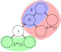
The conditions on $X$ are that it should cover the separator $s_{i}$ and that all its variables should appear in the non-descendants of $i.$ In order to formalize the condition for each node $i\in V,$ we define $\lambda^{de}(i)$ as the set of variables that appear in the scope of the descendants of $i$, namely $\lambda^{de}(i)=\bigcup_{j\in de(i)}\lambda(j)$. Furthermore we define $\lambda^{nde}(i)$ as the set of variables that appear in the scope of the non-descendants of $i,$ namely $\lambda^{nde}(i)=\bigcup_{j\in nde(i)}\lambda(j)$. Figure 1 shows $X$ in blue, $\lambda^{de}(i)$ in green and $\lambda^{nde}(i)$ in red in a simple example to help understanding the notation and the conditions on the lemma.

Lemma 1.

Let $(\Phi,U)$ be a valuation algebra. Let $\Xi\subseteq\Phi$ be a subset of valuations projection-closed and combination-breakable. Let $\phi\in\Xi,$ $\phi=\phi_{1}\times\cdots\times\phi_{n}.$ For any node $i$ of $\mathcal{T},$ and any domain $X\subseteq\lambda^{nde}(i),$ such that $s_{i}\subseteq X,$ we have that $\phi^{\downarrow(X\cup\lambda(i))}$ factorizes as

$$\phi^{\downarrow(X\cup\lambda(i))}=\alpha\times\beta,$$

with $\alpha\in\Xi,$ $d(\alpha)=X$ and $\beta\in\Xi,$ $d(\beta)=\lambda(i).$
Concretely $\alpha=\left(\prod_{j\in nde(i)}\psi_{j}\right)^{\downarrow X}$ and $\beta=\left(\psi_{i}\times\prod_{j\in de(i)}\psi_{j}\right)^{\downarrow\lambda(i)}.$

Proof.

From definition 2, we have that $\phi=\prod_{i\in V}\psi_{i}.$ We can factorize $\phi$ as $\phi=\eta_{1}\times\psi_{i}\times\eta_{2},$ where $\eta_{1}=\prod_{j\in nde(i)}\psi_{j}$ with $d(\eta_{1})=\bigcup_{j\in nde(i)}d(\psi_{j})$ and $\eta_{2}=\prod_{j\in de(i)}\psi_{j}.$ By equation 18 from the appendix, we have that $d(\eta_{2})=\lambda^{de}(i).$

Applying the factorization we have that

$$\phi^{\downarrow(X\cup\lambda(i))} = \left(\eta_{1}\times\psi_{i}\times\eta_{2}\right)^{\downarrow X\cup\lambda(i)}.$$

Since $X\subseteq\lambda^{nde}(i)$, we have that $X\cup\lambda(i)\subseteq\lambda^{nde}(i)\cup\lambda(i)$, and by axiom A4

$$\phi^{\downarrow(X\cup\lambda(i))}=\left(\left(\eta_{1}\times\psi_{i}\times\eta_{2}\right)^{\downarrow\lambda^{nde}(i)\cup\lambda(i)}\right)^{\downarrow X\cup\lambda(i)}.$$

Now $\lambda^{nde}(i)\cup\lambda(i)$ covers both $d(\eta_{1})$ and $d(\psi_{i})$ by the covering property, so we can apply axiom A5 to get

$$\phi^{\downarrow(X\cup\lambda(i))}=\left((\eta_{1}\times\psi_{i})\times\eta_{2}^{\downarrow(\lambda^{nde}(i)\cup\lambda(i))\cap\lambda^{de}(i)}\right)^{\downarrow X\cup\lambda(i)}.$$

Analyzing the domain where $\eta_{2}$ is projected to we find that

$$\left(\lambda^{nde}(i)\cup\lambda(i)\right)\cap\lambda^{de}(i) = \left(\lambda^{nde}(i)\cap\lambda^{de}(i)\right)\cup\left(\lambda(i)\cap\lambda^{de}(i)\right)$$

$$= \left(\lambda(i)\cap\lambda^{de}(i)\right)=\bigcup_{j\in ch(i)}s_{j}$$

where the first equality distributes the intersection, the second one applies that by equation 14 from the appendix we know that $\lambda^{nde}(i)\cap\lambda^{de}(i)\subseteq\lambda(i)\cap\lambda^{de}(i)$ and the third one uses equation 13 also found at the appendix. Replacing in the expression above we get

$$\phi^{\downarrow(X\cup\lambda(i))}=\left(\eta_{1}\times\psi_{i}\times\eta_{2}^{\downarrow\bigcup_{j\in ch(i)}s_{j}}\right)^{\downarrow X\cup\lambda(i)}.$$

Since $\bigcup_{j\in ch(i)}s_{j}\subseteq\lambda(i)$ and $d(\psi_{i})\subseteq\lambda(i)$ we can apply again axiom A5,

$$\phi^{\downarrow(X\cup\lambda(i))}=\eta_{1}^{\downarrow(X\cup\lambda(i))\cap d(\eta_{1})}\times(\psi_{i}\times\eta_{2}^{\downarrow\bigcup_{j\in ch(i)}s_{j}}).$$

From equation 19 from the appendix, we have that $d(\eta_{1})=\lambda^{nde}(i)$ and then

$$\phi^{\downarrow(X\cup\lambda(i))}=\eta_{1}^{\downarrow(X\cup\lambda(i))\cap\lambda^{nde}(i)}\times\psi_{i}\times\eta_{2}^{\downarrow\bigcup_{j\in ch(i)}s_{j}}.$$

Distributing the intersection, we have that $(X\cup\lambda(i))\cap\lambda^{nde}(i)=(X\cap\lambda^{nde}(i))\cup(\lambda(i)\cap\lambda^{nde}(i)).$ In the lemma we required that $X\subseteq\lambda^{nde}(i)$, and from here $X\cap\lambda^{nde}(i)=X$. On the other hand by equation 12, we have that $s_{i}=(\lambda(i)\cap\lambda^{nde}(i))$ and since $s_{i}\subseteq X,$ we get that

$$\phi^{\downarrow(X\cup\lambda(i))}=\eta_{1}^{\downarrow X}\times\psi_{i}\times\eta_{2}^{\downarrow\bigcup_{j\in ch(i)}s_{j}}$$

and applying axiom A5 one last time, this time to join instead of to split, we get

$$\phi^{\downarrow(X\cup\lambda(i))}=\eta_{1}^{\downarrow X}\times\left(\psi_{i}\times\eta_{2}\right)^{\downarrow d(\psi_{i})\cup\bigcup_{j\in ch(i)}s_{j}}.$$

Finally, by equation 1 we have that $\lambda(i)=d(\psi_{i})\cup\bigcup_{j\in ch(i)}s_{j}.$ So, we directly identify that $\phi^{\downarrow X\cup\lambda(i)}$ factorizes as $\alpha\times\beta,$ where $\alpha=\eta_{1}^{\downarrow X}$ and $\beta=\left(\psi_{i}\times\eta_{2}\right)^{\downarrow\lambda(i)},$ with $d(\alpha)=X$ and $d(\beta)=\lambda(i).$

Note that since $\phi\in\Xi$, and $\Xi$ is projection-closed, $\phi^{\downarrow X\cup\lambda(i)}\in\Xi.$ Now, since $\phi^{\downarrow X\cup\lambda(i)}=\alpha\times\beta$, and $\Xi$ is combination-breakable we have that $\alpha\in\Xi,$ and $\beta\in\Xi$. ∎

5.2 Completability properties of extension systems.

In this section we define some properties which will allow us to characterize under which conditions the different algorithms work. Intuitively, these properties impose conditions under which the solution to a “simpler” problem can be completed to obtain a solution to a “more complex” problem.

In this section, let $(\Phi,U)$ be a valuation algebra, $\mathcal{W}$ a extension system and $\Xi\subseteq\Phi$ be a subset of valuations projection-closed and combination-breakable.

Definition 8 (Projective completability).

We say that projective completability (on products) holds on $(\Phi,U),$ $\mathcal{W},$ and $\Xi$ if for each valuation $\phi\in\Xi$ such that $\phi=\xi_{1}\times\xi_{2}$ with domains $d(\xi_{1})=X$ and $d(\xi_{2})=Y$ respectively, for each configuration $\mathbf{x}\in c_{{\phi}^{\downarrow X}}$, we have that each completion of $\mathbf{x}$ to $\phi^{\downarrow Y}$ is a solution of $\phi.$ That is, whenever

$$CO(c_{\phi^{\downarrow X}},\phi^{\downarrow Y})\subseteq c_{\phi}.$$

Corollary 1.

If projective completability holds on $(\Phi,U),$ $\mathcal{W},$ and $\Xi,$ then for each valuation $\phi\in\Xi$ such that $\phi=\xi_{1}\times\xi_{2}$ with domains $d(\xi_{1})=X$ and $d(\xi_{2})=Y$

$$CO(c_{\phi^{\downarrow X}},\phi^{\downarrow Y})=c_{\phi}.$$

Proof.

By definition of projective completability we have that $CO(c_{\phi^{\downarrow X}},\phi^{\downarrow Y})\subseteq c_{\phi}.$

It only remains to prove that $c_{\phi}\subseteq CO(c_{\phi^{\downarrow X}},\phi^{\downarrow Y}).$

Now, for any $\mathbf{s}\in c_{\phi}$ and by applying equation 2 to $c_{\phi}=W_{\phi}^{\emptyset}(\diamond)$ we have that $\mathbf{s}=\langle\mathbf{x},\mathbf{z}\rangle$ where $\mathbf{x}\in c_{\phi^{\downarrow X}}\mbox{ and }\mathbf{z}\in W_{\phi}^{X}(\mathbf{x}).$ Since $c_{\phi^{\downarrow Y}}=c_{\phi}^{\downarrow Y}$ we get $\langle\mathbf{x}^{\downarrow X\cap Y},\mathbf{z}\rangle\in c_{\phi^{\downarrow Y}}.$ Note that $\mathbf{x}\in c_{\phi^{\downarrow X}}$ implies $\mathbf{x}^{\downarrow X\cap Y}\in c_{\phi^{\downarrow X\cap Y}}$ , and applying equation 2 to $c_{\phi^{\downarrow Y}}=W_{\phi^{\downarrow Y}}^{\emptyset}(\diamond),$ we get

$$c_{\phi^{\downarrow Y}}=\{\langle\mathbf{t},\mathbf{z}\rangle|\mathbf{t}\in c_{\phi^{\downarrow X\cap Y}}\mbox{ and }\mathbf{z}\in W_{\phi^{\downarrow Y}}^{X\cap Y}(\mathbf{t})\}$$

we can conclude that $\mathbf{z}\in W_{\phi^{\downarrow Y}}^{X\cap Y}(\mathbf{x}^{\downarrow X\cap Y})$, and hence that $\mathbf{s}\in CO(c_{\phi^{\downarrow X}},\phi^{\downarrow Y})$. ∎

Definition 9 (Piecewise completability).

We say that piecewise completability (on products) holds on $(\Phi,U),$ $\mathcal{W},$ and $\Xi$ if for each valuation $\phi\in\Xi,$ such that $\phi=\xi_{1}\times\xi_{2}$, with domains $X$ and $Y$ respectively, and each $\mathbf{x}\in c_{\phi^{\downarrow X}}$ , each completion of $\mathbf{x}$ to $\xi_{2}$ is a solution of $\phi$ or equivalently

$$CO(c_{\phi^{\downarrow X}},\xi_{2})\subseteq c_{\phi}.$$

We say that piecewise completability is guaranteed non-empty if for each $A$ such that $\emptyset\neq A\subseteq c_{\phi^{\downarrow X}}$, we have that $CO(A,\xi_{2})\neq\emptyset$. Furthermore we say that piecewise completability is total if any solution can be obtained by piecewise completion, that is if $CO(c_{\phi^{\downarrow X}},\xi_{2})=c_{\phi}.$

(a) Projective completion

(b) Piecewise completion

Figure 2: Process of building a solution by completion

5.2.1 Classifying extension systems based on projective and piecewise completability

In this section we investigate the relationship between piecewise and projective completability. Since the proofs for these results rely on valuation algebras on semirings, we only formulate the results here, leaving the proof to the appendix.

Proposition 1.

There are valuation algebras and extension system satisfying:

1. neither projective nor piecewise completability,

2. projective completability but not piecewise completability,

3. piecewise completability but not projective completability,

4. both piecewise and projective completability.

Proof.

See appendix C ∎

5.3 Necessary and sufficient condition for Extend-To-Global-Projection

We start by seeing that the projective completability properties, required only for products of two valuations, can be extended to larger products by virtue of Lemma 1, as long as the conditions imposed by the lemma hold.

Lemma 2.

Assume projective completability holds on $(\Phi,D),$ $\mathcal{W},$ and $\Xi$. Then, given $\phi=\phi_{1}\times\dots\times\phi_{n},$ and any rooted covering join tree $\mathcal{T}=(V,E,\lambda,U)$ for that factorization, for any node $i$ of $V,$ any domain $X\subseteq\lambda^{nde}(i),$ such that $s_{i}\subseteq X,$ we have that $CO(c_{\phi^{\downarrow X}},\phi^{\downarrow\lambda(i)})=c_{\phi^{\downarrow(X\cup\lambda(i))}}.$

Proof.

We can apply Lemma 1 to get that $\phi^{\downarrow(X\cup\lambda(i))}=\alpha\times\beta$, with $d(\alpha)=X$ and $d(\beta)\subseteq\lambda(i).$ Then, we can apply Corollary 1 (with $\phi^{\downarrow(X\cup\lambda(i))}$ in the place of $\phi$ and $\lambda(i)$ in that of $Y$) getting $CO(c_{\phi^{\downarrow X}},\phi^{\downarrow\lambda(i)})=c_{\phi^{\downarrow(X\cup\lambda(i))}}.$

∎

Now, we are ready to establish the sufficient condition for algorithm Extend-To-Global-Projection, which is basically projective completability.

Theorem 5.

Let $(\Phi,U)$ be a valuation algebra, and $\mathcal{W}$ a extension system. Let $\Xi\subseteq\Phi$ be a subset of valuations projection-closed and combination-breakable. Let $\phi\in\Xi,$ and $\mathcal{T}$ a rooted covering join tree for a given factorization $\phi=\phi_{1}\times\dots\times\phi_{n}.$ Let $c$ be the set of configurations assessed by algorithm Extend-To-Global-Projection. If projective completability holds on $\Xi$ then $c=c_{\phi}.$

Proof.

Take as loop invariant $c=c_{\phi^{\downarrow\bigcup_{i\in Visited}\lambda(i)}},$ where $Visited$ is the set of nodes of the join tree that have been visited by the loop up to some point. At the beginning of the first iteration the invariant is satisfied, since $c=\{\diamond\}=c_{\phi^{\downarrow\emptyset}}.$ For the update of $c$ that is made at each interation, the conditions of Lemma 2 are satisfied, and hence, the lemma guarantees that if the invariant is true at the beginning of an iteration, it is true at the end. When the last iteration finishes, we have visited all the nodes and since $d(\phi)=\cup_{i\in V}\lambda(i)$ by Lemma 2, we have that $c=c_{\phi}.$ ∎

In the first counterexample provided in section 3 we had $CO(c_{\phi^{\downarrow X}},\phi^{\downarrow Y})=\Omega_{X\cup Y}$ whereas $c_{\phi}=\{(x\mapsto 0,y\mapsto 0),(x\mapsto 1,y\mapsto 1)\}.$ Thus, projective completability does not hold in that counterexample and hence we do not have any guarantee that the algorithm will work. In the second counterexample as the extension system is derived from this one, projective completability does not hold either. Therefore the misbehaviour of both counterexamples is correctly covered by the new result.

In the next theorem we establish that projective completability is also a necessary condition, in the sense that, if for any product valuation, the algorithm is guaranteed to find a subset of its solutions, then projective completability must hold.

Theorem 6.

Let $(\Phi,U)$ be a valuation algebra, and $\mathcal{W}$ a extension system. Let $\Xi\subseteq\Phi$ be a subset of valuations projection-closed and combination-breakable. If for each valuation $\phi\in\Xi$ which factorizes as $\phi=\xi_{1}\times\xi_{2}$ and for each rooted covering join tree $\mathcal{T}$, Extend-To-Global-Projection  assesses $c$ such that $c\subseteq c_{\phi},$ then projective completability holds on $\Xi$.

Proof.

Assume that Extend-To-Global-Projection  always assesses a subset of $c_{\phi}.$ For any $\phi\in\Xi,$ $\phi=\xi_{1}\times\xi_{2},$ with domains $X$ and $Y$ respectively, we define a covering join tree with two nodes: $v_{1},$ with label $\lambda(v_{1})=X$ covering $\xi_{1},$ and its single child $v_{2},$ with label $\lambda(v_{2})=Y$ covering $\xi_{2}.$ We can run Extend-To-Global-Projection  on $\mathcal{T}$, assessing $c$ which by our assumption will be a subset of $c_{\phi}.$ By manual expansion of the expressions in the algorithm, we see that, for this small tree the solution set assessed is $c=CO(CO(\{\diamond\},\phi^{\downarrow X}),\phi^{\downarrow Y})$. Now, since $c_{\phi^{\downarrow X}}=CO(\{\diamond\},\phi^{\downarrow X})$, we have that $c=CO(c_{\phi^{\downarrow X}},\phi^{\downarrow Y})$ and since we had that $c\subseteq c_{\phi},$ we have that $CO(c_{\phi^{\downarrow X}},\phi^{\downarrow Y})\subseteq c_{\phi}.$ Since this holds for any $\phi\in\Xi,$ $\phi=\xi_{1}\times\xi_{2},$ projective completability must hold. ∎

As noticed by the counterexamples provided in section 3 the necessary and sufficient conditions for the Extend-To-Global-Projection algorithms were not correctly understood in the former literature. We have provided a characterization of the subsets of a valuation algebra where the Extend-To-Global-Projection  algorithm works by means of identifying a sufficient and necessary condition, namely projective completability.

5.4 Necessary and sufficient condition for Extend-To-Subtree

As we did in the previous section, we start by seeing that piecewise completability properties, required only for products of two valuations, can be extended to larger products by virtue of Lemma 1, as long as the conditions imposed by the lemma hold.

Lemma 3.

Let $(\Phi,U)$ be a valuation algebra, and $\mathcal{W}$ a extension system. Let $\Xi\subseteq\Phi$ be a subset of valuations projection-closed and combination-breakable. Then, for any $\phi\in\Xi,$ any rooted covering join tree $\mathcal{T}$ for a given factorization $\phi=\phi_{1}\times\dots\times\phi_{n},$ any node $i$ of $\mathcal{T},$ any domain $X\subseteq\lambda^{nde}(i),$ such that $s_{i}\subseteq X,$ and any set $A\subseteq c_{\phi^{\downarrow X}}$, we define $\beta=\left(\psi_{i}\times\prod_{j\in de(i)}\psi_{j}\right)^{\downarrow\lambda(i)}$ and we have that

1. If piecewise completability holds, then $CO(A,\beta)\subseteq c_{\phi^{\downarrow(X\cup\lambda(i))}},$

2. If piecewise completability is guaranteed non-empty, then whenever $A\neq\emptyset$ we have that $CO(A,\beta)\neq\emptyset.$

3. If piecewise completability is complete we have that $CO(c_{\phi^{\downarrow X}},\beta)=c_{\phi^{\downarrow(X\cup\lambda(i))}}.$

Proof.

We can apply Lemma 1 to get that $\phi^{\downarrow(X\cup\lambda(i))}=\alpha\times\beta$, with $d(\alpha)=X$, $d(\beta)=\lambda(i),$ and $\beta=\left(\psi_{i}\times\prod_{j\in de(i)}\psi_{j}\right)^{\downarrow\lambda(i)}.$ The conditions to apply piecewise completability hold (with $\phi^{\downarrow(X\cup\lambda(i))}$ in place of $\phi$ and $\lambda(i)$ in that of $Y$) getting that $CO(A,\beta)\subseteq c_{\phi^{\downarrow(X\cup\lambda(i))}}.$ The second and third statements can be proven the same way. ∎

Following what we did with Extend-To-Global-Projection, now we are ready to establish the sufficient contitions for the Extend-To-Subtree  algorithm, namely piecewise completability in its different flavors.

Theorem 7.

Let $(\Phi,U)$ be a valuation algebra, and $\mathcal{W}$ a extension system. Let $\Xi\subseteq\Phi$ be a subset of valuations projection-closed and combination-breakable. Let $\phi\in\Xi,$ and $\mathcal{T}$ be a rooted covering join tree for a given factorization $\phi=\phi_{1}\times\dots\times\phi_{n}.$ Let $c$ be the set of configurations assessed by algorithm Extend-To-Subtree. We have that

1. If piecewise completability holds on $\Xi$, then $c$ is a subset of $c_{\phi}.$

2. If piecewise completability is guaranteed non-empty on $\Xi$ then also $c\neq\emptyset$.

3. If piecewise completability is total on $\Xi$, then $c=c_{\phi}.$

Proof.

To prove statement 1, take as loop invariant $c\subseteq c_{\phi^{\downarrow\bigcup_{i\in Visited}\lambda(i)}},$ where $Visited$ is the set of nodes of the join tree that have been visited by the loop up to some point. At the beginning of the first iteration the invariant is satisfied, since $c=\{\diamond\}\subseteq c_{\phi^{\downarrow\emptyset}}.$ For the update of $c$ that is made at each interation, the conditions of Lemma 3 are satisfied, and hence, the lemma guarantees that if the invariant is true at the beginning of an iteration, it is true at the end. When the last iteration finishes, we have visited all the nodes and since Lemma 2 shows that $d(\phi)=\cup_{i\in V}\lambda(i),$ we have that $c\subseteq c_{\phi}.$ Statements 2 and 3 can be proven the same way. ∎

Again, piecewise completability is not only a sufficient condition, but also necessary if the Extend-To-Subtree  algorithm works in a consistent manner, as proven by the following theorem.

Theorem 8.

Let $(\Phi,U)$ be a valuation algebra, and $\mathcal{W}$ a extension system. Let $\Xi\subseteq\Phi$ be a subset of valuations projection-closed and combination-breakable. If for each valuation $\phi\in\Xi,$ $\phi=\xi_{1}\times\xi_{2}$ and for each rooted covering join tree $\mathcal{T}$, Extend-To-Subtree assesses $c$ such that

1. $c\subseteq c_{\phi},$ then piecewise completability holds on $\Xi$.

2. $\emptyset\neq c\subseteq c_{\phi},$ then piecewise completability is guaranteed non-empty on $\Xi$.

3. $c=c_{\phi},$ then piecewise completability is total on $\Xi$.

Proof.

We start proving statement 1. Assume that Extend-To-Subtree  always assesses a subset of $c_{\phi}.$ Given $\phi\in\Xi,$ $\phi=\xi_{1}\times\xi_{2},$ with domains $X$ and $Y$ respectivelty, we define a join tree with two nodes: $v_{1},$ with label $\lambda(v_{1})=X$ covering $\xi_{1},$ and its single child $v_{2},$ with label $\lambda(v_{2})=Y$ covering $\xi_{2}.$ We can run Extend-To-Subtree-Projections on $\mathcal{T}$, getting $c\subseteq c_{\phi}.$ However in this particular case we can see that $c=CO(CO(\{\diamond\},\phi^{\downarrow X}),\xi_{2})$. Now, since $c_{\phi^{\downarrow X}}=CO(\{\diamond\},\phi^{\downarrow X})$, we have that $c=CO(c_{\phi^{\downarrow X}},\xi_{2})$. Since the algorithm is guaranteed to return $c\subseteq c_{\phi},$ piecewise completability must hold. Statements 2 and 3 can be proven the same way. ∎

5.5 Sufficient conditions for Single-Extend-To-Subtree

Finally, we show that the Single-Extend-To-Subtree  algorithm can be applied if guaranteed non-empty piecewise completability holds.

Theorem 9.

Let $(\Phi,U)$ be a valuation algebra, and $\mathcal{W}$ a extension system. Let $\Xi\subseteq\Phi$ be a subset of valuations projection-closed and combination-breakable. Let $\phi\in\Xi,$ and $\mathcal{T}$ be a rooted covering join tree for a given factorization $\phi=\phi_{1}\times\dots\times\phi_{n}.$ If guaranteed non-empty piecewise completability holds on $\Xi$, then Single-Extend-To-Subtree  assesses a configuration $\mathbf{x}$ which is a solution to $\phi.$

Proof.

Take as loop invariant $\mathbf{x}\in c_{\phi^{\downarrow\bigcup_{i\in Visited}\lambda(i)}},$ where $Visited$ is the set of nodes of the join tree that have been visited by the loop up to some point. At the beginning of the first iteration the invariant is satisfied, since $\diamond\in c_{\phi^{\downarrow\emptyset}}.$ The update of $\mathbf{x}$ that made at each interation, is possible because the conditions of Lemma 3 (including guaranteed non-emptyness) are satisfied, and hence, there is a completion that we can select, store in $\mathbf{x},$ and it is guaranteed to maintain the invariant. When the last iteration finishes, we have visited all the nodes and since $d(\phi)=\cup_{i\in V}\lambda(i)$ due to Lemma 2, we have that $\mathbf{x}\in c_{\phi}.$ ∎

In the last three sections we have characterized under which circumstances can we apply each algorithm. In the next section we compare with the sufficient conditions provided by Pouly and Kohlas.

5.6 Alternative proofs for the PK results

As we argued before, Pouly and Kohlas stated that Extend-To-Global-Projection  always assessed $c_{\phi},$ and we disproved by means of counterexamples. However, we have proven that projective completability is a sufficient and necessary condition for the algorithm. They did also provide sufficient conditions for the algorithms Extend-To-Subtree  and Single-Extend-To-Subtree. We will see that, although the proofs relied on a disproved theorem, the results provided were correct. We do that by proving that the sufficient conditions established by them and described in section 4.1 imply our sufficient conditions.

As can be seen in Table 1, CPK1 and CPK2 were proposed as sufficient condition for Extend-To-Subtree  to assess some solutions and for Single-Extend-To-Subtree  to assess a solution. The following lemma allows us to use theorems 7 and 9 to prove that their conditions were indeed sufficient.

Lemma 4.

Assume that conditions CPK1 and CPK2 hold. Then, guaranteed non-empty piecewise completability holds on $\Phi$.

Proof.

Take $\xi_{1},\xi_{2}\in\Phi$, with domains $X$ and $Y$ respectively, and let $\phi=\xi_{1}\times\xi_{2}.$ To prove piecewise completability,we have to prove that $CO(c_{\phi^{\downarrow X}},\xi_{2})\subseteq c_{\phi}.$ Now by definition $CO(c_{\phi^{\downarrow X}},\xi_{2})=\{(\mathbf{x},\mathbf{z})\mid\mathbf{x}\in c_{\phi^{\downarrow X}}\mbox{ and }\mathbf{z}\in W_{\xi_{2}}^{X\cap Y}(\mathbf{x}^{\downarrow X\cap Y})\}.$ We can apply CPK2 to get $CO(c_{\phi^{\downarrow X}},\xi_{2})\subseteq\{(\mathbf{x},\mathbf{z})\mid\mathbf{x}\in c_{\phi^{\downarrow X}}\mbox{ and }\mathbf{z}\in W_{\phi}^{X}(\mathbf{x})\}.$ Now, by the second condition in the definition of extension system we get $CO(c_{\phi^{\downarrow X}},\xi_{2})\subseteq\{(\mathbf{x},\mathbf{z})\mid\mathbf{x}\in c_{\phi^{\downarrow X}}\mbox{ and }\mathbf{z}\in W_{\phi}^{X}(\mathbf{x})\}=W_{\phi}^{\emptyset}(\diamond)=c_{\phi}$ and piecewise completability is proven. Now we need to see that non-emptyness is guaranteed. Take $A$ such that $\emptyset\neq A\subseteq c_{{\phi}^{\downarrow X}}$, we have to prove that $CO(A,\xi_{2})\neq\emptyset.$ Again by definition $CO(A,\xi_{2})=\{(\mathbf{x},\mathbf{z})\mid\mathbf{x}\in A\mbox{ and }\mathbf{z}\in W_{\xi_{2}}^{X\cap Y}(\mathbf{x}^{\downarrow X\cap Y})\}$. By CPK1 we have that $W_{\xi_{2}}^{X\cap Y}(\mathbf{x}^{\downarrow X\cap Y})\neq\emptyset$ and so $CO(A,\xi_{2})$ is guaranteed to be non-empty. ∎

Furthermore, CPK1 and CPK3 were identified as a sufficient condition for Extend-To-Subtree  to assess $c_{\phi}.$ The following lemma allows us to use theorems 7 and 9 to prove that their conditions were indeed sufficient.

Lemma 5.

Assume that conditions CPK1 and CPK3 hold. Then, total piecewise completability holds on $\Phi$.

Proof.

Take $\xi_{1},\xi_{2}\in\Phi$, with domains $X$ and $Y$ respectively, and let $\phi=\xi_{1}\times\xi_{2}.$ To prove piecewise total completability, we have to prove that $CO(c_{\phi^{\downarrow X}},\xi_{2})=c_{\phi}.$ Now by definition $CO(c_{\phi^{\downarrow X}},\xi_{2})=\{(\mathbf{x},\mathbf{z})\mid\mathbf{x}\in c_{\phi^{\downarrow X}}\mbox{ and }\mathbf{z}\in W_{\xi_{2}}^{X\cap Y}(\mathbf{x}^{\downarrow X\cap Y})\}.$ We can apply CPK3 to get $CO(c_{\phi^{\downarrow X}},\xi_{2})=\{(\mathbf{x},\mathbf{z})\mid\mathbf{x}\in c_{\phi^{\downarrow X}}\mbox{ and }\mathbf{z}\in W_{\phi}^{X}(\mathbf{x})\}.$ Now, by the second condition in the definition of extension system we get $CO(c_{\phi^{\downarrow X}},\xi_{2})=\{(\mathbf{x},\mathbf{z})\mid\mathbf{x}\in c_{\phi^{\downarrow X}}\mbox{ and }\mathbf{z}\in W_{\phi}^{X}(\mathbf{x})\}=W_{\phi}^{\emptyset}(\diamond)=c_{\phi}$ and total piecewise completability is proven. ∎

On the other hand, we point out that in both cases the sufficient conditions we require, while similar to the ones required by Pouly and Kohlas are strictly weaker than those. In particular, their conditions need to hold on any configuration $\mathbf{x}\in\Omega_{X},$ whilst we only require them to hold for those $\mathbf{x}\in c_{\phi^{\downarrow X}}.$ That is, while they impose conditions on the extension of tuples which are not solutions, we restrict ourselves to solutions. Table 3 summarizes the results in this section, providing the sufficient conditions for each algorithm, whether the condition has also been proven to be also necessary and whether the condition we require is weaker than the one previously required.

Algorithm	Suff. cond.	Nec. cond.	Weaker	Solutions
3	Projective completability	Yes	-	All
5	Guaranteed non-empty piecewise completability	No	Yes	One
4	Guaranteed non-empty piecewise completability	Yes	Yes	Some
4	Total piecewise completability	Yes	Yes	All

Table 3: Sufficient and necessary conditions of the generic algorithms.

6 Optimization problems in semiring induced valuation algebras

Many problems in Artificial Intelligence can be expressed in terms of a particular type of valuations, namely semiring induced valuation algebras, that emerge from a mapping from tuples to the values of a commutative semiring [6, 5, 17, 30]. Particularly interesting are optimization problems, where the semiring is selective. We start by reviewing optimization problems and the result that an extension system can be defined when the semiring is selective. Then, by means of a counterexample, we show that the sufficient condition imposed by Pouly and Kohlas for the correctness of Extend-To-Global-Projection  is not correct and propose a sufficient condition and a necessary condition for projective completability to hold on valuation algebras imposed by a selective semiring, and thus, for Extend-To-Global-Projection  to work. Later, for Single-Extend-To-Subtree  and Extend-To-Subtree  we provide correct proofs for the sufficient conditions introduced by Pouly and Kohlas to solve the single and partial SFP. Finally we show that we can weaken the sufficient condition proposed by Pouly and Kohlas for Extend-To-Subtree to solve the complete SFP from strict monotonicity to weak cancellativity. Furthermore we show that weak cancellativity is also a necessary condition.

6.1 Optimization problems.

We start by defining some basic abstract algebra structures needed to specify the problem and then we formally state the problem, which is a particular case of the SFP.

Definition 10.

A semiring is a set $R$ equipped with two binary operations $+$ and $\cdot$, called addition and multiplication, such that (i) $+$ is an associative and commutative operation with identity element $0$, (ii) $\cdot$ is an associative operation with identity element $1$, (iii) multiplication left and right distributes over addition, that is $a\cdot(b+c)=(a\cdot b)+(a\text{$\cdot$}c)$ and $(a+b)\cdot c=(a\cdot c)+(b\cdot c)$, and (iv) multiplication by 0 annihilates $R$, that is $a\cdot 0=0\cdot a=0$.

If $\cdot$ is commutative then $(R,+,\cdot)$ is a commutative semiring.

Theorem 10.

Let $\langle U,\Omega\rangle$ be a variable system, and $(R,+,.)$ a commutative semiring. A semiring valuation $\phi$ with domain $X\subseteq U$ is a function $\phi:\Omega_{X}\rightarrow R.$ The set of all semiring valuations with domain $X$ is noted $\Phi_{X}$, and $\Phi=\bigcup_{X\subseteq U}\Phi_{X}.$ Now we define $d(\phi)=X$ if $\phi\in\Phi_{X}.$ Furthermore $(\phi\times\psi)(\mathbf{x})=\phi(\mathbf{x}^{\downarrow d(\phi)})\cdot\psi(\mathbf{x}^{\downarrow d(\psi)}).$ And finally $\phi^{\downarrow Y}(\mathbf{y})=\sum_{\mathbf{z}\in\Omega_{d(\phi)-Y}}\phi(\langle\mathbf{y},\mathbf{z}\rangle)$ for $Y\subseteq d(\phi)$. With these operations, $(\Phi,U)$ satisfies the axioms of a valuation algebra and is called the valuation algebra induced by $(R,+,.)$ in $\langle U,\Omega\rangle$.

Proof.

See Theorem PK5.2. ∎

Thus, in the following we are only interested in commutative semirings. Note that Example 1 is indeed a semiring induced valuation algebra.

Definition 11.

For any semiring induced valuation algebra, the optimization solution concept assigns at each $\phi\in\Phi_{X},$ the set of solutions $c_{\phi}=\{\mathbf{x}\in\Omega_{X}|\phi(\mathbf{x})=\phi^{\downarrow\emptyset}(\diamond)\}.$ Thus we define the single (resp. partial, complete) optimization solution finding problem as the single (resp. partial, complete) solution finding problem with this solution concept on the valuation algebra induced by that semiring.

The former definition of optimization problem covers several common optimization formalisms, such as Classical Optimization, Satisfiability, Maximum Satisfability, Most & Least Probable Values, Bayesian and Maximum Likelihood decoding and Linear decoding. Details can be found in [23].

6.2 A extension system for optimization.

We are interested in determining whether we can use the algorithms presented in section 3.2. The first requirement for those algorithms was the existence of an extension system, which we will prove in this section. In order to define an extension system, we need to impose a condition on the semiring, namely being selective.

Definition 12.

A semiring is $(R,+,\cdot)$ is selective if for all $a,b\in R,$ either $a+b=a$ or $a+b=b$.

In a selective semiring, we can define a relation

$$a\leq b\Longleftrightarrow a+b=b.$$

As a consequence of Proposition 3.4.7 in [13], in any selective semiring $\leq$ is a total order relation. It is immediate to see that in any selective semiring $a+b=\max\{a,b\}$, where the maximum is taken with respect to the total order $\leq.$ Note that, since $0$ is the sum’s identity, we have that $0\leq a$ for all $a.$

Definition 13.

Given the valuation algebra induced by a selective semiring, we define the optimization extension system as the family of sets obtained by defining the set of extensions of $\mathbf{x}$ to $\phi,$ where $\mathbf{x\in\Omega}_{X}$ and $X\subseteq d(\phi)$, as

$$W_{\phi}^{X}(\mathbf{x})=\{\mathbf{z}\in\Omega_{d(\phi)-X}|\phi(\langle\mathbf{x},\mathbf{z}\rangle)=\phi^{\downarrow X}(\mathbf{x})\}.$$ (9)

Notice that $W_{\phi}^{\emptyset}(\diamond)$ is equal to $c_{\phi}$ as defined by the optimization solution concept.

Lemma 6.

The optimization extension system satisfies the condition in equation 2 and hence, it is an extension system.

Proof.

We want to prove $W_{\phi}^{X}(\mathbf{x})=\{\langle\mathbf{y},\mathbf{z}\rangle|\mathbf{y}\in W_{\phi^{\downarrow Y}}^{X}(\mathbf{x})\mbox{ and }\mathbf{z}\in W_{\phi}^{Y}(\langle\mathbf{x},\mathbf{y}\rangle)\}$ for $X\subseteq Y\subseteq d(\phi).$ In order to simplify the notation take $A=\{\langle\mathbf{y},\mathbf{z}\rangle|\mathbf{y}\in W_{\phi^{\downarrow Y}}^{X}(\mathbf{x})\mbox{ and }\mathbf{z}\in W_{\phi}^{Y}(\mathbf{x},\mathbf{y})\}.$

It follows from equation 9 that

$$A = \{\langle\mathbf{y},\mathbf{z}\rangle\mid\phi^{\downarrow X}(\mathbf{x})=\phi^{\downarrow Y}(\langle\mathbf{x},\mathbf{y}\rangle)\mbox{ and $\phi^{\downarrow Y}$($\langle\mathbf{x}$,$\mathbf{y}\rangle$=}\phi(\langle\langle\mathbf{x},\mathbf{y}\rangle,\mathbf{z}\rangle)\}$$ (10)

$$= \{\langle\mathbf{y},\mathbf{z}\rangle\mid\phi^{\downarrow X}(\mathbf{x})=\phi^{\downarrow Y}(\langle\mathbf{x},\mathbf{y}\rangle)=\phi(\langle\langle\mathbf{x},\mathbf{y}\rangle,\mathbf{z}\rangle)\}.$$

For any $\mathbf{t}\in A$ we have that $\mathbf{t}=\langle\mathbf{y},\mathbf{z}\rangle$ with $\mathbf{y}\in\Omega_{Y-X}$ and $\mathbf{z}\in\Omega_{d(\phi)-(X\cup Y)}$, therefore $\mathbf{t}\in\Omega_{d(\phi)-X}$. Hence, the domain of the tuples in $A$ and $W_{\phi}^{X}(\mathbf{x})$ are actually the same.

• We prove that $A\subseteq W_{\phi}^{X}(\mathbf{x}).$ Take $\mathbf{t}\in A$. We have that $\mathbf{t}=\langle\mathbf{y},\mathbf{z}\rangle,$ and by equation 10 that $\phi^{\downarrow X}(\mathbf{x})=\phi(\langle\langle\mathbf{x},\mathbf{y}\rangle,\mathbf{z}\rangle).$ Now, by the associativity of the concatenation of tuples we have that $\phi^{\downarrow X}(\mathbf{x})=\phi(\langle\langle\mathbf{x},\langle\mathbf{y},\mathbf{z}\rangle\rangle)=\phi(\langle\mathbf{x},\mathbf{t}\rangle),$ proving that $\mathbf{t}\in W_{\phi}^{X}(\mathbf{x}).$

• We prove that $W_{\phi}^{X}(\mathbf{x})\subseteq A.$ Take $\mathbf{t}\in W_{\phi}^{X}(\mathbf{x})$. From the definition of $W_{\phi}^{X}(\mathbf{x}),$ we have

  $$\begin{array}[]{c}\phi(\langle\mathbf{x},\mathbf{t}\rangle)=\phi^{\downarrow X}(\mathbf{x})=\sum_{\mathbf{z}\in\Omega_{d(\phi)-X}}\phi(\langle\mathbf{x},\mathbf{z}\rangle)\mbox{, and }\\ \phi^{\downarrow Y}(\langle\mathbf{x},\mathbf{t}^{\downarrow Y-X}\rangle)=\sum_{\mathbf{z^{\prime}}\in\Omega_{d(\phi)-Y}}\phi(\langle\langle\mathbf{x},\mathbf{t}^{\downarrow Y-X}\rangle,\mathbf{z^{\prime}}\rangle).\end{array}$$

  Since our semiring is selective, we can apply that $a+b=\max\{a,b\}$, to obtain

  $$\begin{array}[]{c}\begin{array}[]{ccc}\phi(\langle\mathbf{x},\mathbf{t}\rangle)&=&\max_{\mathbf{z}\in\Omega_{d(\phi)-X}}\phi(\langle\mathbf{x},\mathbf{z}\rangle)\mbox{, and }\\ \phi^{\downarrow Y}(\langle\mathbf{x},\mathbf{t}^{\downarrow Y-X}\rangle)&=&\max_{\mathbf{z}\in\Omega_{d(\phi)-Y}}\phi(\langle\langle\mathbf{x},\mathbf{t}^{\downarrow Y-X}\rangle,\mathbf{z}\rangle)\\ &=&\max_{\mathbf{z}\in\Omega_{d(\phi)-Y}}\phi(\langle\mathbf{x},\langle\mathbf{t}^{\downarrow Y-X},\mathbf{z}\rangle\rangle).\end{array}\end{array}$$

  Then $\phi(\langle\mathbf{x},\mathbf{t}\rangle)\leq\max_{\mathbf{z}\in\Omega_{d(\phi)-Y}}\phi(\langle\mathbf{x},\langle\mathbf{t}^{\downarrow Y-X},\mathbf{z}\rangle\rangle)=\phi^{\downarrow Y}(\langle\mathbf{x},\mathbf{t}^{\downarrow Y-X}\rangle).$ On the other hand

  $$\phi^{\downarrow Y}(\langle\mathbf{x},\mathbf{t}^{\downarrow Y-X}\rangle) = \max_{\mathbf{z}\in\Omega_{d(\phi)-Y}}\phi(\langle\mathbf{x},\langle\mathbf{t}^{\downarrow Y-X},\mathbf{z}\rangle\rangle)$$

  $$\leq \max_{\mathbf{z}\in\Omega_{d(\phi)-X}}\phi(\langle\mathbf{x},\mathbf{z}\rangle)=\phi^{\downarrow X}(\mathbf{x})=\phi(\langle\mathbf{x},\mathbf{t}\rangle),$$

  which, since the order is total, proves $\phi^{\downarrow Y}(\langle\mathbf{x},\mathbf{t}^{\downarrow Y-X}\rangle)=\phi(\langle\mathbf{x},\mathbf{t}\rangle)=\phi^{\downarrow X}(\mathbf{x})$ and hence $\mathbf{t}\in A.$

∎

The extension system defined in Example 2 is an optimization extension system.

6.3 Necessary and sufficient conditions for Extend-To-Global-Projection on optimization problems

Pouly and Kohlas claimed that Extend-To-Global-Projection  solves the complete optimization SFP on any valuation algebra induced by a commutative selective semiring. The following counterexample shows that this is not correct.

Counterexample 3.

There are valuation algebras induced by selective semirings where Extend-To-Global-Projection  does not solve the optimization complete SFP.

Proof.

We start by defining a commutative selective semiring over the subset of integers $R=\{0,1,2,3\}$. The sum is defined as the maximum of the two integers, that is $a+b=$$\max(a,b).$ The product is defined by the following table

$\cdot$	0	1	2	3
0	0	0	0	0
1	0	1	2	3
2	0	2	2	3
3	0	3	3	3

It is easy to check directly that $(R,\max,\cdot)$ is a commutative selective semiring.

Now, we take two boolean variables $x$ and $y$ and define the valuations:

$$\phi_{1}(x)=\begin{cases}2&\mbox{, if }x=0\\ 3&\mbox{, if }x=1\end{cases} \phi_{2}(y)=\begin{cases}2&\mbox{, if }y=0\\ 3&\mbox{, if }y=1.\end{cases}$$

The product $\phi=\phi_{1}\times\phi_{2},$ is $\phi(x,y)=\begin{cases}2&\mbox{, if }x=y=0\\ 3&\mbox{, otherwise.}\end{cases}$

The solutions of $\phi$ are the assignments $\{\{x\mapsto 0,y\mapsto 1\},\{x\mapsto 1,y\mapsto 0\},\{x\mapsto 1,y\mapsto 1\}\}.$ However, the result of running algorithm Extend-To-Global-Projection  will include the assignment $\{x\mapsto 0,y\mapsto 0\}$ which is not a solution.

∎

The need to identify a sufficient condition where the algorithm solves the complete optimization SFP arises as a consequence of the counterexample. Note that we have already identified a sufficient and necessary condition in section 5.3, namely projective completability. What we would like to see is whether we can transform this condition into a condition of the semiring. We will start by defining two conditions on a semiring and seeing that for commutative semirings, one implies the other. Then, we will prove that the stronger condition is sufficient and that the weaker condition is necessary.

Definition 14.

A selective semiring $(R,+,\cdot)$ is square multiplicatively cancellative on image if for each $a,b\in Im(\cdot),$ $a\neq 0,$ having $a\cdot a=b\cdot a$ implies $a=b.$

A selective semiring $(R,+,\cdot)$ is square ordered if for each $a,b\in R,$ having $a\cdot a=b\cdot a$ implies that $b\cdot b\geq a\cdot a.$

Proposition 2.

If a selective semiring is commutative and square multiplicatively cancellative on image then it is square ordered.

Proof.

By reductio ad absurdum. Let’s assume that $(R,+,\cdot)$ is not square ordered. This means that there are $a,b\in R$ such that $a\cdot a=b\cdot a$ and $b\cdot b<a\cdot a.$ Now, take $c=a\cdot a$ and $d=b\cdot b$. These are two elements in $Im(\cdot)$ and since $b\cdot b<a\cdot a,$ we have that $c=a\cdot a>b\cdot b\geq 0.$ Also, notice that $c\cdot c=a\cdot a\cdot a\cdot a$. Since $a\cdot a=b\cdot a$, we get that $c\cdot c=b\cdot a\cdot b\cdot a$ and since the semiring is commutative, we have that $c\cdot c=b\cdot b\cdot a\cdot a=d\cdot c$. So, applying that R is square multiplicatively cancellative on image, we get that $c=d$, that is $a\cdot a=b\cdot b,$ which contradicts that $b\cdot b<a\cdot a.$ ∎

Theorem 11.

Let $(\Phi,U)$ be a valuation algebra induced by a selective commutative semiring $(R,+,\cdot)$. If $(R,+,\cdot)$ is square multiplicatively cancellative on image, then projective extensibility holds on $\Phi.$

Proof.

We start by assuming that the semiring is square multiplicatively cancellative on image and we see that projective completability holds. We have to prove that for any valuation $\phi=\phi_{1}\times\phi_{2}$ with $d(\phi_{1})=X$ and $d(\phi_{2})=Y$ we have that $CO(c_{\phi^{\downarrow X}},\phi^{\downarrow Y})\subseteq c_{\phi}$. To make the notation simpler the value of the solution, namely $\phi^{\downarrow\emptyset}(\diamond),$ will be written as $M.$

If $M=\phi^{\downarrow\emptyset}(\diamond)=0$ then $\phi(\mathbf{t})=0$ for all $\mathbf{t}\in\Omega_{d(\phi)}$, since $\phi^{\downarrow\emptyset}(\diamond)=\sum_{\mathbf{t}\in\Omega_{d(\phi)}}\phi(\mathbf{t})=\max_{\mathbf{t}\in\Omega_{d(\phi)}}\phi(\mathbf{t})$, and $0$ is the minimal element. Hence, all the configurations are solutions, and $CO(c_{\phi^{\downarrow X}},\phi^{\downarrow Y})\subseteq\Omega_{d(\phi)}=c_{\phi},$ and projective completability is guaranteed.

So we only need study the case when $M\neq 0.$ In that case, take $\langle\mathbf{x},\mathbf{z}\rangle\in CO(c_{\phi^{\downarrow X}},\phi^{\downarrow Y}).$ By definition of completion we have that $\mathbf{x}\in c_{\phi^{\downarrow X}}$ and $\mathbf{z}\in W_{\phi^{\downarrow Y}}^{X\cap Y}(\mathbf{x}^{\downarrow X\cap Y}).$ By definition of $c_{\phi^{\downarrow X}}$, for any $\mathbf{x}\in c_{\phi^{\downarrow X}}$ we have $\phi^{\downarrow X}(\mathbf{x})=\phi^{\downarrow\emptyset}(\diamond)=M,$ and hence we have that $\phi^{\downarrow X\cap Y}(\mathbf{x}^{\downarrow X\cap Y})=M.$

Furthermore, if $\mathbf{z}\in W_{\phi^{\downarrow Y}}^{X\cap Y}(\mathbf{x}^{\downarrow X\cap Y}),$ by equation 9, we have $\phi^{\downarrow Y}(\mathbf{\langle x}^{\downarrow X\cap Y},\mathbf{z\rangle})=\phi^{\downarrow X\cap Y}(\mathbf{x}^{\downarrow X\cap Y}),$ and since from the previous paragraph we have that $\phi^{\downarrow X\cap Y}(\mathbf{x}^{\downarrow X\cap Y})=M,$ we can conclude that $\phi^{\downarrow Y}(\mathbf{\langle x}^{\downarrow X\cap Y},\mathbf{z\rangle})=M.$ In order to finish the proof we need to see that $\langle\mathbf{x},\mathbf{z}\rangle\in c_{\phi}.$

By using the combination axiom we have

$$M=\phi^{\downarrow\emptyset}(\diamond)=\phi^{\downarrow X}(\mathbf{x})=(\phi_{1}\times\phi_{2})^{\downarrow X}(\mathbf{x})=\phi_{1}(\mathbf{x})\cdot\phi_{2}^{\downarrow X\cap Y}(\mathbf{x}{}^{\downarrow X\cap Y})$$

and

$$M = \phi^{\downarrow\emptyset}(\diamond)=\phi^{\downarrow Y}(\langle\mathbf{x}{}^{\downarrow X\cap Y},\mathbf{z\rangle})=(\phi_{1}\times\phi_{2})^{\downarrow Y}(\langle\mathbf{x}{}^{\downarrow X\cap Y},\mathbf{z}\rangle)=$$

$$= \phi_{1}^{\downarrow X\cap Y}(\mathbf{x}^{\downarrow X\cap Y})\cdot\phi_{2}(\langle\mathbf{x}^{\downarrow X\cap Y},\mathbf{z}\rangle)$$

Hence

$$M\cdot M = \phi_{1}(\mathbf{x})\cdot\phi_{2}^{\downarrow X\cap Y}(\mathbf{x}^{\downarrow X\cap Y})\cdot\phi_{1}^{\downarrow X\cap Y}(\mathbf{x}^{\downarrow X\cap Y})\cdot\phi_{2}(\langle\mathbf{x}^{\downarrow X\cap Y},\mathbf{z\rangle})$$

$$= \phi_{1}(\mathbf{x})\cdot\phi_{2}(\langle\mathbf{x}^{\downarrow X\cap Y},\mathbf{z}\rangle)\cdot\phi_{2}^{\downarrow X\cap Y}(\mathbf{x}^{\downarrow X\cap Y})\cdot\phi_{1}^{\downarrow X\cap Y}(\mathbf{x}^{\downarrow X\cap Y})$$

$$= \phi(\langle\mathbf{x},\mathbf{z}\rangle)\ \ \ \ \ \ \ \ \ \ \ \ \ \ \ \ \ \ \cdot\phi(\mathbf{x}^{\downarrow X\cap Y})$$

$$= \phi(\langle\mathbf{x},\mathbf{z}\rangle)\cdot M$$

Now, we have that $M\neq 0$ and that both $M$ and $\phi(\langle\mathbf{x},\mathbf{z}\rangle)$ are in $Im(\cdot),$ since by definition $\phi=\phi_{1}\times\phi_{2}.$ By applying that $(R,+,\cdot)$ is square multiplicatively cancellative on image we have that $\phi(\langle\mathbf{x},\mathbf{z}\rangle)=M,$ which proves $\langle\mathbf{x},\mathbf{z}\rangle\in c_{\phi}.$∎

Theorem 12.

Let $(\Phi,U)$ be a valuation algebra induced by a selective commutative semiring $(R,+,\cdot)$. If the valuation algebra has two variables that can take two or more values, and projective extensibility holds on $\Phi$, then $(R,+,\cdot)$ is square ordered.

Proof.

To prove it we will generalize counterexample 3. Assume the semiring is not square ordered. This means that there are $a,b\in R$ such that $a\cdot a=b\cdot a$ and $b\cdot b<a\cdot a.$ Let $x,y$ be two variables with two or more variables.
Define $\phi_{X}(x)=\begin{cases}b&\mbox{ if }x=0\\ a&\mbox{ if }x=1\\ 0&\mbox{ otherwise.}\end{cases}$ and $\phi_{Y}(y)=\begin{cases}b&\mbox{ if }y=0\\ a&\mbox{ if }y=1\\ 0&\mbox{ otherwise.}\end{cases}$
Let $\phi=\phi_{X}\times\phi_{Y}.$ We have that $\phi(x,y)=\begin{cases}b\cdot b&\mbox{ if }x=y=0\\ a\cdot a&\mbox{ if }(x,y)\in\{(1,1),(0,1),(1,0)\}\\ 0&\mbox{ otherwise.}\end{cases}$

Now, from the definition of projection, $\phi^{\downarrow X}(x)=\begin{cases}a\cdot a&\mbox{ if }x=0\mbox{ or }x=1\\ 0&\mbox{ otherwise.}\end{cases}$ and $\phi^{\downarrow Y}(y)=\begin{cases}a\cdot a&\mbox{ if }y=0\mbox{ or }y=1\\ 0&\mbox{ otherwise.}\end{cases}$

Clearly projective completability does not hold in this example, since the solutions are $\{\{x\mapsto 0,y\mapsto 1\},\{x\mapsto 1,y\mapsto 0\},\{x\mapsto 1,y\mapsto 1\}\}$ and by projective completability we also find $\{x\mapsto 0,y\mapsto 0\}$. ∎

6.4 Piecewise completability on optimization problems

In Theorem 7 we have shown that piecewise completability is the sufficient condition for Extend-To-Subtree solving the partial optimization SFP. Furthermore, non-empty piecewise completability is the necessary condition for Single-Extend-To-Subtree  solving the single SFP. In this section we show that the optimization extension system guarantees non-empty piecewise completability. As a consequence, we can use Single-Extend-To-Subtree  to find a solution and Extend-To-Subtree  to find some solutions in any optimization SFP.

Theorem 13.

The optimization extension system satisfies non-empty piecewise completability on $\Phi$.

Proof.

Take a valuation $\phi=\xi_{1}\times\xi_{2}$ where $\xi_{1},\xi_{2}\in\Phi$, with domains $X$ and $Y$ respectively. We have to prove that $CO(c_{\phi^{\downarrow X}},\xi_{2})\subseteq c_{\phi}.$

By definition of set of completions, we have that

$$CO(c_{\phi^{\downarrow X}},\xi_{2})=\{\langle\mathbf{x},\mathbf{z}\rangle|\mathbf{x}\in c_{\phi^{\downarrow X}}\text{ and }\mathbf{z}\in W_{\xi_{2}}^{X\cap Y}(\mathbf{x}^{\downarrow X\cap Y})\}.$$

Now, from the definition of $c_{\phi},$ we have that

$$c_{\phi}=W_{\phi}^{\emptyset}(\diamond)=\{\langle\mathbf{x},\mathbf{z\rangle})|\mathbf{x}\in c_{\phi^{\downarrow X}}\text{ and }\mathbf{z}\in W_{\xi_{1}\times\xi_{2}}^{X}(\mathbf{x})\}.$$

So, piecewise completability is satisfied if, and only if, for each $\mathbf{x}\in c_{\phi^{\downarrow X}},$ we have that $W_{\xi_{2}}^{X\cap Y}(\mathbf{x}^{\downarrow X\cap Y})\subseteq W_{\xi_{1}\times\xi_{2}}^{X}(\mathbf{x}).$

Now take $\mathbf{z}\in W_{\xi_{2}}^{X\cap Y}(\mathbf{x}^{\downarrow X\cap Y}).$ From the definition we have that $\xi_{2}(\langle\mathbf{x}^{\downarrow X\cap Y},\mathbf{z}\rangle)=\xi_{2}^{\downarrow X\cap Y}(\mathbf{x}^{\downarrow X\cap Y}).$ Multiplying by $\xi_{1}(\mathbf{x})$ we get that

$$\xi_{1}(\mathbf{x})\cdot\xi_{2}(\langle\mathbf{x}^{\downarrow X\cap Y},\mathbf{z}\rangle)=\xi_{1}(\mathbf{x})\cdot\xi_{2}^{\downarrow X\cap Y}(\mathbf{x}^{\downarrow X\cap Y}).$$ (11)

Next, we have that

$$(\xi_{1}\times\xi_{2})(\mathbf{x},\mathbf{z}) = \xi_{1}(\mathbf{x})\cdot\xi_{2}(\langle\mathbf{x}^{\downarrow X\cap Y},\mathbf{z}\rangle)=\xi_{1}(\mathbf{x})\cdot\xi_{2}^{\downarrow X\cap Y}(\mathbf{x}^{\downarrow X\cap Y})$$

$$= (\xi_{1}\times\xi_{2}^{\downarrow X\cap Y})(\mathbf{x})=(\xi_{1}\times\xi_{2})^{\downarrow X}(\mathbf{x}).$$

where the first equality is the definition of combination, the second is equation 11, and the remaining are basic valuation algebra manipulations

But now, since $W_{\xi_{1}\times\xi_{2}}^{X}(\mathbf{x})=$$\{\mathbf{z}\in\Omega_{d(\phi)-X}|(\xi_{1}\times\xi_{2})(\mathbf{x},\mathbf{z})=(\xi_{1}\times\xi_{2})^{\downarrow X}(\mathbf{x})\}$, it is clear that $\mathbf{z}\in W_{\xi_{1}\times\xi_{2}}^{X}(\mathbf{x}).$ Hence , $W_{\xi_{2}}^{X\cap Y}(\mathbf{x}^{\downarrow X\cap Y})\subseteq W_{\xi_{1}\times\xi_{2}}^{X}(\mathbf{x}).$

Since the optimization extension system is a total implementation of a solution concept which is guaranteed non-empty, $c_{\phi^{\downarrow X}}$ is non-empty and by the definition of extension set in equation 9, the set of extensions cannot be empty, hence $CO(c_{\phi^{\downarrow X}},\xi_{2})$ is non-empty. This provides guaranteed non-empty piecewise completability. ∎

As a result of Theorem 13, non-empty piecewise completability is guaranteed on any optimization extension system. In Theorem 8 we have seen that total piecewise completability is a necessary and sufficient condition for Extend-To-Subtree  to solve the complete SFP. We are interested in characterizing for which semirings does the optimization extension system satisfy total piecewise completability. Theorem 13 proved non-empty piecewise completability on $\text{$\Phi$}.$ It turns out that it is not possible to extend this result to total piecewise completability. However, sometimes the completability conditions only hold for a subset of the valuations and this is the case here. We will see that total piecewise completability does only hold if the valuation $\phi$ for which we try to find a solution has at least one configuration whose value is not zero. However to do that first we take a detour to talk about valuation algebras with null elements.

Definition 15.

An element $0_{X}\in\Phi_{X}$ is a null element if

1. For each $\phi\in\Phi_{X},$ we have $\phi\times 0_{X}=0_{X}\times\phi=0_{X}.$

2. For $X\subseteq Y\subseteq U$ and $\phi\in\Phi_{Y},$ we have that $\phi^{\downarrow X}=0_{X}$ if and only if $\phi=0_{Y}.$

Lemma 7.

In a valuation algebra, the set $NN\subseteq\Phi$ of non-null elements is projection-closed and combination-breakable.

Proof.

From the second condition in Definition 15, we have that the set of non-null elements is projection-closed. To prove that it is combination breakable pick any $\phi$ that is non-null and such that $\phi=\xi_{1}\times\xi_{2}.$ Now assume that either $\xi_{1}$ or $\xi_{2}$ is null. Then by the first condition in Definition 15 we have that $\phi$ is null which is a contradiction. Hence, both $\xi_{1}$ and $\xi_{2}$ must be non-null. ∎

In selective semiring induced valuation algebras, a valuation $\phi$ is null if and only if $\phi^{\downarrow\emptyset}(\diamond)=0.$ Thus, all possible configurations in $\mbox{$\Omega$}_{d(\phi)}$ are solutions. Since Extend-To-Subtree  runs the Collect algorithm as a previous step, it is easy to determine whether $\phi$ is constant $0$ by assessing $\phi^{\downarrow\emptyset}(\diamond)=\left(\psi_{r}^{\prime}\right)^{\downarrow\emptyset}(\diamond)$ and checking whether it is equal to $0.$ In that case we can directly return $\Omega_{d(\phi)}$. Thus, we can easily identify and solve null valuations. So, we have to concentrate on when does total piecewise completability hold on $NN.$ Next, we define weak multiplicative cancellativity and prove that it is the sufficient and necessary condition on a semiring for Extend-To-Subtree to solve the complete optimization SFP.

Definition 16.

A commutative semiring $R$ is weakly multiplicatively cancellative if for any $a,b,c\in R,$ we have that

$$a\cdot c\neq 0\mbox{, and }a\cdot c=b\cdot c\,\,\,\,\,\,\,\,\,\,\,\,\,\,\,\,\,\,\,\mbox{ implies that \,\,\,\,\,\,\,\,\,\,\,\,\,\,\,\,\,\,\,\,$a=b$.}$$

Theorem 14.

Let $R$ be a commutative selective semiring. If $R$ is weakly multiplicatively cancellative then its induced valuation algebra satisfies total piecewise completability on $NN$. On the other hand, if the valuation algebra has one variable that can take two or more values, and total piecewise completability on $NN$ is satisfied, then $R$ is weakly multiplicatively cancellative.

Proof.

We start proving that, if the semiring is weakly multiplicatively cancellative, we have total piecewise completability on $NN.$ Take a valuation $\phi=\xi_{1}\times\xi_{2}$ where $\xi_{1},\xi_{2}\in\Phi$, with domains $X$ and $Y$ respectively. We have to prove that $CO(c_{\phi^{\downarrow X}},\xi_{2})=c_{\phi}.$

By definition of set of completions, we have that

$$CO(c_{\phi^{\downarrow X}},\xi_{2})=\{(\mathbf{x},\mathbf{z})|\mathbf{x}\in c_{\phi^{\downarrow X}}\text{ and }\mathbf{z}\in W_{\xi_{2}}^{X\cap Y}(\mathbf{x}^{\downarrow X\cap Y})\}.$$

Now, from the definition of $c_{\phi},$ we have that

$$c_{\phi}=W_{\phi}^{\emptyset}(\diamond)=\{(\mathbf{x},\mathbf{z})|\mathbf{x}\in c_{\phi^{\downarrow X}}\text{ and }\mathbf{z}\in W_{\xi_{1}\times\xi_{2}}^{X}(\mathbf{x})\}.$$

So, total piecewise completability is satisfied if, and only if, for each $\mathbf{x}\in c_{\phi^{\downarrow X}},$ we have that $W_{\xi_{2}}^{X\cap Y}(\mathbf{x}^{\downarrow X\cap Y})=W_{\xi_{1}\times\xi_{2}}^{X}(\mathbf{x}).$

In Theorem 13, we proved that $W_{\xi_{2}}^{X\cap Y}(\mathbf{x}^{\downarrow X\cap Y})\subseteq W_{\xi_{1}\times\xi_{2}}^{X}(\mathbf{x}).$ Thus, it remains to prove that $W_{\xi_{1}\times\xi_{2}}^{X}(\mathbf{x})\subseteq W_{\xi_{2}}^{X\cap Y}(\mathbf{x}^{\downarrow X\cap Y}).$

Now take $\mathbf{z}\in W_{\xi_{1}\times\xi_{2}}^{X}(\mathbf{x}).$ From the definition we have that $(\xi_{1}\times\xi_{2})(\mathbf{x},\mathbf{z})=(\xi_{1}\times\xi_{2})^{\downarrow X}(\mathbf{x}).$ From here,

$$(\xi_{1}\times\xi_{2})(\mathbf{x},\mathbf{z})=(\xi_{1}\times\xi_{2}^{\downarrow X\cap Y})(\mathbf{x})$$

and by definition of combination

$$\xi_{1}(\mathbf{x})\cdot\xi_{2}((\mathbf{x}^{\downarrow X\cap Y},\mathbf{z}))=\xi_{1}(\mathbf{x})\cdot\xi_{2}^{\downarrow X\cap Y}(\mathbf{x}).$$

We have that $\xi_{1}(\mathbf{x})\cdot\xi_{2}^{\downarrow X\cap Y}(\mathbf{x})=\phi^{\downarrow X}(\mathbf{x})=\phi^{\downarrow\emptyset}(\diamond)\neq 0,$ where the second equality follows because $\mathbf{x}\in c_{\phi^{\downarrow X}},$ and the third one since $\phi\in NN,$ and hence $\phi^{\downarrow\emptyset}(\diamond)\neq 0.$ So we can apply weak cancellation to $\xi_{1}(\mathbf{x})$ getting

$$\xi_{2}((\mathbf{x}^{\downarrow X\cap Y},\mathbf{z}))=\xi_{2}^{\downarrow X\cap Y}(\mathbf{x}^{\downarrow X\cap Y}).$$

But this is exactly the condition that $\mathbf{z}$ has to satisfy in order to be in $W_{\xi_{2}}^{X\cap Y}(\mathbf{x}^{\downarrow X\cap Y}).$ We have proven that $W_{\xi_{1}\times\xi_{2}}^{X}(\mathbf{x})\subseteq W_{\xi_{2}}^{X\cap Y}(\mathbf{x}^{\downarrow X\cap Y})$ and in Theorem 13, we proved that $W_{\xi_{2}}^{X\cap Y}(\mathbf{x}^{\downarrow X\cap Y})\subseteq W_{\xi_{1}\times\xi_{2}}^{X}(\mathbf{x}).$ Thus, $W_{\xi_{2}}^{X\cap Y}(\mathbf{x}^{\downarrow X\cap Y})=W_{\xi_{1}\times\xi_{2}}^{X}(\mathbf{x}).$

The second part of the proof assumes total piecewise completability on $NN$ and concludes that the semiring must be weakly multiplicatively cancellative. To prove it, we assume that it is not and will reach a contradiction. Let $a,b,c\in R,$ such that $a\cdot c\neq 0,$ $a\cdot c=b\cdot c$ and $a\neq b.$ Now, we build a valuation which has as domain a single variable $\mathbf{x}$ with at least two values, namely $x_{0}$ and $x_{1}.$

$$\phi(\mathbf{x})=(\xi_{1}\times\xi_{2})(\mathbf{x})$$

with

$$\xi_{1}(\diamond)=c,$$

and

$$\xi_{2}(\mathbf{x})=\begin{cases}a&\mbox{\ if $\mathbf{x}=x_{0}$,}\\ b&\ \mbox{if $\mathbf{x}=x_{1},$}\\ 0&\ \mbox{otherwise.}\end{cases}$$

Note that $\phi$ is non-null and that the set of solutions of $\phi$ is $\{x_{0},x_{1}\}.$ Now, if $a>b,$ then $W_{\xi_{2}}^{\emptyset}(\diamond)=\{x_{0}\},$ and the only solution found by piecewise completing will be $\{x_{0}\}.$ On the other hand, if $b>a$, then then $W_{\xi_{2}}^{\emptyset}(\diamond)=\{x_{1}\},$ and the only solution found by piecewise completing will be $\{x_{1}\}.$ Thus, in both cases we get to a contradiction. ∎

Table 4 summarizes the results in this section, providing the sufficient and necessary conditions for each algorithm. We have proven a sufficient condition to Extend-To-Global-Projection, which correctly deals with counterexample 3. For Extend-To-Subtree to solve the complete optimization SFP, Pouly and Kohlas required strict monotonicity which, for selective semirings, is equivalent to multiplicative cancellativity (see Proposition 3). We have proven that weakly multiplicative cancellativity suffices. Furthermore, where possible, we have provided also necessary conditions.

Algorithm	Problem	Semiring suff. cond.	Semiring nec. cond.
3	Complete optimization SFP	Square multiplicatively cancellative on image	Square ordered
5	Single optimization SFP	None	None
4	Partial optimization SFP	None	None
4	Complete optimization SFP	Weakly multiplicatively cancellative	Weakly multiplicatively cancellative

Table 4: Sufficient and necessary conditions on optimization problems (semirings considered are always commutative and selective).

7 Conclusions

The theory for the generic construction of solutions in valuation based systems [22, 23] studies three widely used dynamic programming algorithms from the most general perspective and provides necessary conditions for those algorithms to be correct. We have presented counterexamples to the results presented there and we have shown that the counterexamples have a deep impact in the theory. This has opened the way for identifying two properties of extension systems: projective completability and piecewise completability. We have proven that such properties constitute sufficient and necessary conditions for those generic algorithms to be correct, allowing for a sharper characterization of when each algorithmic scheme can be applied. To the best of our knowledge, up to know no necessary conditions for these generic algorithms had been presented in the literature.

A particularly interesting case where these algorithms can be applied is valuation algebras induced by a commutative selective semiring, where they constitute the base of well known optimization algorithms. For that case, we have also corrected a result in [22, 23]. Furthermore, we have been able to translate the sufficient and necessary conditions for the algorithms into conditions for the semiring, identifying three new semiring properties: square multiplicatively cancellative on image, square ordered and weakly multiplicatively cancellative. Although we have started scratching the relationships between these semiring properties, a deeper study of their interactions remains as future work.

As a result, our corrected theory provides the more general description of these generic algorithms and the sharpest characterization to date of their necessary and sufficient conditions.

A Properties of rooted covering join trees

We prove some poperties of rooted covering join trees which are needed to ease the proofs of the results presented in the paper. In any rooted join tree, for each node $i\in V,$ we define $\lambda^{de}(i)$ as the set of variables that appear in the scope of the descendants of $i$, namely $\lambda^{de}(i)=\bigcup_{j\in de(i)}\lambda(j)$. Furthermore we define $\lambda^{nde}(i)$ as the set of variables that appear in the scope of the non-descendants of $i,$ namely $\lambda^{nde}(i)=\bigcup_{j\in nde(i)}\lambda(j)$.

Lemma 8.

For any node $i$ of $V$

$$s_{i}=\lambda(i)\cap\lambda^{nde}(i)$$ (12)

$$\bigcup_{j\in ch(i)}s_{j}=\lambda(i)\cap\lambda^{de}(i)$$ (13)

$$\lambda^{nde}(i)\cap\lambda^{de}(i)\subseteq\lambda(i)\cap\lambda^{de}(i)$$ (14)

Proof.

We start proving equation 12. If $i$ is the root, then $s_{i}=\emptyset$ and the equation is trivially satisfied. Assume that $i$ is not the root. By definition of $\lambda^{nde}(i)$, we have that $\lambda(i)\cap\lambda^{nde}(i)=\lambda(i)\cap\bigcup_{j\in nde(i)}\lambda(j)=\bigcup_{j\in nde(i)}(\lambda(i)\cap\lambda(j))=s_{i}\cup\bigcup_{j\in nde(i)-\{p_{i}\}}(\lambda(i)\cap\lambda(j)).$ For any $j\in nde(i)-\{p_{i}\},$ we have that $p_{i}$ lies in the path between $j$ and $i$, and by the running intersection property, $\lambda(i)\cap\lambda(j)\subseteq\lambda(p_{i})$. Since $\lambda(i)\cap\lambda(j)\subseteq\lambda(i),$ we have that $\lambda(i)\cap\lambda(j)\subseteq\lambda(i)\cap\lambda(p_{i})=s_{i}.$ Thus, $\bigcup_{j\in nde(i)-\{p_{i}\}}\lambda(i)\cap\lambda(j)\subseteq s_{i},$ and $\lambda(i)\cap\lambda^{nde}(i)=s_{i}.$

Next, we will prove equation 13

$$\lambda(i)\cap\lambda^{de}(i) = \lambda(i)\cap\bigcup_{j\in de(i)}\lambda(j)=\lambda(i)\cap\bigcup_{j\in ch(i)}[\lambda(j)\cup\bigcup_{k\in de(j)}\lambda(k)]$$

$$= \bigcup_{j\in ch(i)}[(\lambda(i)\cap\lambda(j))\cup\bigcup_{k\in de(j)}(\lambda(i)\cap\lambda(k))].$$

Now, by the running intersection property, $\lambda(i)\cap\lambda(k)\subseteq\lambda(i)\cap\lambda(j),$ so we can remove the union $\bigcup_{k\in de(j)}(\lambda(i)\cap\lambda(k))$ leaving

$$\lambda(i)\cap\lambda^{de}(i)=\bigcup_{j\in ch(i)}[\lambda(i)\cap\lambda(j)]=\bigcup_{j\in ch(i)}s_{j}.$$

Finally, we will conclude by proving equation 14. Applying the definitions we have that $\lambda^{nde}(i)\cap\lambda^{de}(i)=\left(\bigcup_{j\in nde(i)}\lambda(j)\right)\cap\left(\bigcup_{k\in de(i)}\lambda(k)\right)=\bigcup_{j\in nde(i)}\bigcup_{k\in de(i)}\lambda(j)\cap\lambda(k).$ But now node $i$ lies in the path between any node $j$ which is non-descedant of $i$ and any other node $k$ which is descendant of $i.$ Thus, by the running intersection property we have that $\lambda(j)\cap\lambda(k)\subseteq\lambda(i),$ and that $\bigcup_{j\in nde(i)}\bigcup_{k\in de(i)}\lambda(j)\cap\lambda(k)\subseteq\lambda(i).$ From here we have that $\lambda^{nde}(i)\cap\lambda^{de}(i)\subseteq\lambda(i)\cap\lambda^{de}(i).$ ∎

B Minimally labeled covering join trees

In the paper we make the assumption that covering join trees are minimally labeled (see Assumption 1). In this appendix we start by checking that, for a fixed tree, there is no covering join tree whose labels are smaller that those of a minimally labeled join tree. Afterwards, we prove that it is easy to build a minimally labeled covering join tree provided a tree and a valuation assignment function. Finally we prove some properties of minimally labeled covering join trees which are used in the proofs in the paper.

We start by proving that there can be no labelling smaller than that of a minimally labeled covering join tree.

Lemma 9.

Let ($V,E)$ be a tree. Given a valuation $\phi=\phi_{1}\times\cdots\times\phi_{n},$ there is no covering join tree $\mathcal{T}=(V,E,\lambda,U)$, valuation assignment $a$, $i\in V,$ and $k\in ne(i),$ such that $\lambda(i)\nsupseteq d(\psi_{i})\cup\bigcup_{j\in ne(i)\setminus\{k\}}s_{ij}.$

Proof.

The proof is immediate since $s_{ij}=\lambda(i)\cap\lambda(j)\subseteq\lambda(i)$ and $d(\psi_{i})\subseteq\lambda(i)$ is required for $a$ to be a valuation assignment. ∎

Now, Algorithm 6 provides a procedure to assess a minimally labeled covering join tree provided a covering join tree and a valuation assignment $a.$

1:for all nodes $i$ of $\mathcal{T}$ do

2:    $\alpha(i):=\bigcup_{j\in a^{-1}(i)}d(\phi_{j})$

3:    $\beta(i):=\alpha(i)$

4:    $\gamma(i):=\emptyset$

5:end for

6:for all nodes $i$ of $\mathcal{T}$ except the root in an upward order  do

7:    $\alpha(p_{i}):=\alpha(p_{i})\cup\alpha(i)$

8:    $\beta(p_{i}):=\beta(p_{i})\cup(\gamma(p_{i})\cap\alpha(i))$

9:    $\gamma(p_{i}):=\gamma(i)\cup\alpha(i)$

10:end for

11:$\lambda(r):=\beta(r)$

12:for all nodes $i$ of $\mathcal{T}$ except the root in an downward order  do

13:    $\lambda(i):=\beta(i)\cup(\lambda(p_{i})\cap\alpha(i))$

14:end for

15:return $\boldsymbol{\lambda}$;

Algorithm 6 MinimalLambdas algorithm

Lemma 10.

MinimalLambdas asseses a minimally labeled covering join tree. Furthermore MinimalLambdas only requires time and space $O(|V||U|),$ where $V$ is the set of nodes of the join tree and $U$ is the set of variables of the problem.

Proof.

We will start proving that MinimalLambdas asseses a covering join tree. Let $\phi=\phi_{1},\dots,\phi_{n}$ be a valuation and let $\mathcal{\mathcal{T}}=(V,E,\lambda,U)$ be a tree where the MinimalLambdas algorithm has been run. After the second loop we have

$$\begin{array}[]{c}\alpha(i)=d(\psi_{i})\cup\left(\bigcup_{j\in de(i)}d(\psi_{j})\right)\end{array} \beta(i)=d(\psi_{i})\cup\left(\bigcup_{\begin{subarray}{c}{j,k\in ch(i)}\\ j\neq k\end{subarray}}\alpha(j)\cap\alpha(k)\right).$$ and (16)

Notice that $\beta(i)\subseteq\alpha(i)$ and as a consequence $\lambda(i)=\beta(i)\cup\left(\lambda(p_{i})\cap\alpha(i)\right)\subseteq\alpha(i)\cup\left(\lambda(p_{i})\cap\alpha(i)\right)\subseteq\alpha(i).$ Also notice that for any $i\in de(j)$, $\alpha(i)\subseteq\alpha(j).$ After the third loop we get $\lambda(i)=\beta(i)\cup(\lambda(p_{i})\cap\alpha(i)).$ Thus, $\lambda(p_{i})\cap\alpha(i)\subseteq\lambda(i).$

Next we will prove that the runing intersection property is satisfied. Let $n_{1},n_{2},\dots,n_{m}$ be the unique path between two given nodes $n_{1},n_{m}\in V$. We want to see that $\lambda(n_{1})\cap\lambda(n_{m})\subseteq\lambda(n_{i}),$ for $1<i<m$. Notice that if $m\leq 2$ it is trivially true. Therefore we will suppose $m\geq 3$. As long as $\mathcal{T}$ is a tree, the previous path can be seen as the composition of two different paths, one ascending path which grows up from $n_{1}$ up to $n_{i}$ with $1\leq i\leq m$, and one descending path from $n_{i}$ to $n_{m}$. That is $n_{j+1}=p_{n_{j}}$ for $1\leq j\leq i-1$ and $n_{j+1}\in ch(n_{j})$ for $i\leq j\leq m-1.$ Notice that if $n_{1}\neq n_{m}$ at most one of these subpaths may be empty. Hence there are three possible configurations for the paths either the descending path is empty, or the ascending path is empty or no subpath is empty. Equivalently, either $i=m$ or $i=1$ or $1\lneq i\lneq m$.

1. Assume that the descending path is empty, so $i=m$. We have that $\lambda(n_{1})\cap\lambda(n_{m})\subseteq\lambda(n_{1})\subseteq\alpha(n_{1})\subseteq\alpha(n_{m-1})$ and $\lambda(n_{1})\cap\lambda(n_{m})\subseteq\lambda(n_{m})=\lambda(p_{n_{m-1}}).$ In conclusion we obtain $\lambda(n_{1})\cap\lambda(n_{m})\subseteq\alpha(n_{m-1})\cap\lambda(p_{n_{m-1}})\subseteq\lambda(n_{m-1})$, and we have verificed that $n_{m-1}$ fulfills the condition. Now since, by induction we have that $\lambda(n_{1})\cap\lambda(n_{m})\subseteq\lambda(n_{j}),$ for $1<j<m.$

2. In case the ascending path is empty we can consider the path from $n_{m}$ to $n_{1}$ and use the previous argument, since $n_{m},n_{m-1},\dots,n_{1}$ is an ascending path.

3. Finally, if no subpath is empty it holds that $1\lneq i\lneq m.$ In this case, we have that $\lambda(n_{1})\subseteq\alpha(n_{1})\subseteq\alpha(n_{i-1})$ and $\lambda(n_{m})\subseteq\alpha(n_{m})\subseteq\alpha(n_{i+1})$. Since $n_{i-1},n_{i+1}\in ch(n_{i})$ we obtain: $\lambda(n_{1})\cap\lambda(n_{m})\subseteq\alpha(n_{i-1})\cap\alpha(n_{i+1})\subseteq{\displaystyle\bigcup_{\begin{subarray}{c}{j,k\in ch(i)}\\ j\neq k\end{subarray}}\alpha(j)\cap\alpha(k)\subseteq\beta(i)\subseteq\lambda(i)},$ and thus the condition is fulfilled for $i.$ As long as $n_{1},\dots,n_{i}$ is an ascending path and $n_{i},\dots,n_{m}$ is a descending path, we can use the previous cases to check that $\lambda(n_{1})\cap\lambda(n_{i})\subseteq\lambda(n_{j})$ for $1\leq j\leq m,$ which concludes the proof since $\lambda(n_{1})\cap\lambda(n_{m})=\lambda(n_{1})\cap\lambda(n_{m})\cap\lambda(n_{i})\subseteq\lambda(n_{1})\cap\lambda(n_{i})\subseteq\lambda(n_{j}).$

We have just shown that $\mathcal{T}$ is a join tree, but as long as for all $\psi(i)$ it is satisfied $d(\psi_{i})\subseteq\lambda(i)$ we also have that $\mathcal{T}$ is actually a covering join tree.

Next, we will prove that $\mathcal{T}$ is minimally labeled. By lemma 9 we already know that $\lambda(i)\supseteq d(\psi_{i})\cup\bigcup_{j\in ne(i)\setminus\{k\}}s_{ij}$ for all $i\in V$. We will prove by contradiction that $\lambda(i)=d(\psi_{i})\cup\bigcup_{j\in ne(i)\setminus\{k\}}s_{ij}.$ Assume that for some $i\in V$ there is a variable $x\in\lambda(i)$ and a $k^{\prime}\in ne(i)$ such that $x\notin d(\psi_{i})\cup\bigcup_{j\in ne(i)\setminus\{k^{\prime}\}}s_{ij}.$ Since $\lambda(i)=\beta(i)\cup(\lambda(p_{i})\cap\alpha(i))$, we have that $x\in\beta(i)$ or $x\in\lambda(p_{i})\cap\alpha(i).$

1. If $x\in\beta(i),$ since by assumption $x\notin d(\psi_{i}),$ we can conclude from equation 16 that $x\in\bigcup_{\begin{subarray}{c}{j,k\in ch(i)}\\ j\neq k\end{subarray}}\alpha(j)\cap\alpha(k)$. Nonetheless, if there are $j,k\in ch(i)$ such that $x\in\lambda(j)$ and $x\in\lambda(k)$, then by the running intersection property $x\in\lambda(i)$ and as a consequence $x\in s_{i,j}$ and $x\in s_{ik}.$ For any possible value of $k^{\prime},$ either $s_{ij}$ or $s_{ik}$ will be part of $\bigcup_{j\in ne(i)\setminus\{k^{\prime}\}}s_{ij}.$, and thus, we have a contradiction.

2. If $x\in\lambda(p_{i})\cap\alpha(i)$. We have $x\in\alpha(i)=d(\psi_{i})\cup\left(\bigcup_{j\in de(i)}d(\psi_{j})\right)$ and $x\in\lambda(p_{i})$. Since by assumption $x\notin d(\psi_{i}),$ then $x\in\bigcup_{j\in de(i)}d(\psi_{j}).$ Nevertheless, $x\in\bigcup_{j\in de(i)}d(\psi_{j})$ implies $x\in\bigcup_{j\in de(i)}\lambda(j)$, and by the running intersection property, there must exist at least one $j\in ch(i)$ such that $x\in\lambda(j)$, in particular $x\in s_{i,j}$, which also contradicts our hypothesis since $x\in\lambda(p_{i})$ implies $x\in s_{i,p_{i}}$.

∎

B.1 Basic properties of minimally labeled covering join trees

In the following, let $\mathcal{\mathcal{T}}=(V,E,\lambda,U)$ be a minimally labeled covering join tree.

Removing any edge $\{i,j$} on the $\mathcal{T}$, breaks it into two different trees: $\mathcal{T}_{i}^{-j},$ the one containing $i$ and $\mathcal{T}_{j}^{-i},$the one containing $j.$

Lemma 11.

For any edge $\{i,j\}$ of $\mathcal{T}$,

$$\bigcup_{k\in\mathcal{T}_{i}^{-j}}\lambda(k)=d(\prod_{k\in\mathcal{T}_{i}^{-j}}\psi_{k})$$ (17)

Proof.

We can place $i$ at the root and use induction on the height of the tree.

If $i$ is a leaf, then it is trivially true, since both sides are $d(\psi_{i})$.

Let $i$ be a node with height $n$ and assume it is true whenever the height is smaller than $n.$ Each node in $\mathcal{T}_{i}$ lies in a subtree rooted at one of the children of $i,$ so $\bigcup_{k\in\mathcal{T}_{i}^{-j}}\lambda(k)=\lambda(i)\cup\left(\bigcup_{j^{\prime}\in ne(i)-\{j\}}\bigcup_{k^{\prime}\in\mathcal{T}_{j^{\prime}}^{-i}}\lambda(k^{\prime})\right)$ Now applying the minimally labeled assumption to $\lambda(i)$ with $k=j$ we get $\lambda(i)=d(\psi_{i})\cup\bigcup_{j^{\prime}\in ne(i)-\{j\}}s_{ij^{\prime}}.$ Thus,$\bigcup_{k\in\mathcal{T}_{i}^{-j}}\lambda(k)=d(\psi_{i})\cup\left(\bigcup_{j^{\prime}\in ne(i)-\{j\}}s_{ij^{\prime}}\cup\bigcup_{k^{\prime}\in\mathcal{T}_{j^{\prime}}^{-i}}\lambda(k^{\prime})\right).$ By definition each separator $s_{ij^{\prime}}\subseteq\lambda(j^{\prime}),$ and hence $s_{ij^{\prime}}\subseteq\bigcup_{k^{\prime}\in\mathcal{T}_{j^{\prime}}^{-i}}\lambda(k^{\prime}),$ so we can remove the $s_{ij^{\prime}}$ from the previous expression, getting $\bigcup_{k\in\mathcal{T}_{i}^{-j}}\lambda(k)=d(\psi_{i})\cup\left(\bigcup_{j^{\prime}\in ne(i)-\{j\}}\bigcup_{k^{\prime}\in\mathcal{T}_{j^{\prime}}^{-i}}\lambda(k^{\prime})\right).$ Now we can apply the induction hypothesis on each children $j$, getting $\bigcup_{k^{\prime}\in\mathcal{T}_{j^{\prime}}^{-i}}\lambda(k^{\prime})=d(\prod_{k^{\prime}\in\mathcal{T}_{j^{\prime}}^{-i}}\psi_{k^{\prime}})$ and the proof is finished.∎

Corollary 2.

Let $\phi=\phi_{1}\times\dots\times\phi_{n}$ be a valuation and let $\mathcal{\mathcal{T}}=(V,E,\lambda,U)$ a minimally labeled covering join tree for this factorization. Then, $d(\phi)=\bigcup_{i\in V}\lambda(i)$.

Proof.

By induction on the height of the tree, parallel to the one of the previous Lemma. ∎

Lemma 12.

For any node $i$ of $V,$

$$\lambda^{de}(i)=d(\prod_{j\in de(i)}\psi_{j})$$ (18)

Proof.

Every descendant of $i$ lies on the subtree of one of its childs. Thus, $\lambda^{de}(i)=\bigcup_{j\in ch(i)}\bigcup_{k\in\mathcal{T}_{j}^{-i}}\lambda(k)$ and by direct application of Lemma 11 we get $\lambda^{de}(i)=\bigcup_{j\in ch(i)}d(\prod_{k\in\mathcal{T}_{j}^{-i}}\psi_{k}))=d(\prod_{j\in ch(i)}\prod_{k\in\mathcal{T}_{j}^{-i}}\psi_{k}))=d(\prod_{j\in de(i)}\psi_{j}).$ ∎

Lemma 13.

For any node $i$ of $V,$

$$\lambda^{nde}(i)=d(\prod_{j\in nde(i)}\psi_{j})$$ (19)

Proof.

Directly applying Lemma 11 to the link $\{p_{i},j\},$ since the set of nodes in $\mathcal{T}_{p_{i}}^{-i}$ is exactly $nde(i).$ ∎

C Piecewise and projective extensibility

In this section we concentrate on proving proposition 1. Let us start by recalling it. See 1

We will provide an example of valuation algebras and extension system in each of the four categories.

A simple example of valuation algebra and extension system such that none of the completabilities are satisfied is the one provided in counterexample 2. As for the fourth category, any valuation algebra induced by the semiring $(\mathbb{R},\max,\cdot)$ satisfies both piecewise and projective extensibility. The valuation algebra presented in counterexample 3 satisfies piecewise completability but does not satisfy projective completability. Next, we provide an example of valuation algebra satisfying projective completability but not piecewise completability.

Let $U=\{x,y\}$ be a set with two variables. Let $D_{x}=D_{y}=\{0,1\}$ and $\Omega$ the set of all tuples. We have that $\langle U,\Omega\rangle$ are a variable system. Consider the valuation algebra induced by the semiring $(\mathbb{R},\max,+)$. Let $\phi_{1}:\Omega_{X}\rightarrow\mathbb{R}$, and $\phi_{2}:\Omega_{Y}\rightarrow\mathbb{R},$ be two valuations defined as

$$\begin{array}[]{ccc}\phi_{1}((x\mapsto 0))=2&&\phi_{2}((y\mapsto 0))=2\\ \phi_{1}((x\mapsto 1))=1&&\phi_{2}((y\mapsto 1))=1\end{array}$$

Taking $\Psi=\{\phi_{1}^{a}\times\phi_{2}^{b}\times(\phi_{1}^{\downarrow\emptyset})^{c}\times(\phi_{2}^{\downarrow\emptyset})^{d}\}$, it is easy to prove that $(\Psi,U)$ fulfils the axioms of a valuation algebra.

Next, we have to define the extension sets in $(\Psi,U^{\prime})$. We will build a new extension system $\mathcal{\overline{W}}$ in the following way:

• For $\phi_{1}$ we define its extensible solutions $\overline{W}_{\phi_{1}}^{\emptyset}(\diamond)=\overline{c}_{\phi_{1}}=\{(x\mapsto 0),(x\mapsto 1)\}$

• For $\phi_{2}$ we define $\overline{W}_{\phi_{1}}^{\emptyset}(\diamond)=\overline{c}_{\phi_{2}}=\{(y\mapsto 0),(y\mapsto 1)\}.$

• For any other valuation $\psi\in\Psi$, with $d(\psi)=X$ we define $\overline{W}_{\psi}^{\emptyset}(\diamond)=\overline{c}_{\psi}=\{(x\mapsto 0)\}.$

• For any other valuation $\psi\in\Psi$, with $d(\psi)=Y$ we define $\overline{W}_{\psi}^{\emptyset}(\diamond)=\overline{c}_{\psi}=\{(y\mapsto 0)\}.$

• For any other valuation $\psi\in\Psi$, with $d(\psi)=X\cup Y$ we define $\overline{W}_{\psi}^{\emptyset}(\diamond)=\overline{c}_{\psi}=\{((x,y)\mapsto(0,0))\}.$

This definition guarantees that $\overline{\mathcal{W}}$ is an extension system on $(\Psi,U).$

We will now see that the valuation algebra $(\Psi,U)$ with extension system $\overline{\mathcal{W}}$ satisfies projectitve extensibility but does not satisfy piecewise extensibility.

For any valuation with domain $X$ it is immediate to prove that it is projective extensible since there is no domain $\emptyset\subsetneq D\subsetneq X$. Same holds for any valuation with domain $Y.$

For any valuation $\psi$, such that $d(\psi)=X\cup Y$ we have $\overline{c}_{\psi}=\{((x,y)\mapsto(0,0))\}.$ Additionaly it holds $\overline{c}_{\psi^{\downarrow X}}=\{(x\mapsto 0)\}$ and $\overline{c}_{\psi^{\downarrow Y}}=\{(y\mapsto 0)\}$. In particular we have that$\psi$ is projective extenible.

We have just shown that all the valuations in $(\Psi,U)$ are projective extensible. Hence we only have to find a valuation which is not piecewise extensible. Let $\phi=\phi_{1}\times\phi_{2}$. Since $\overline{c}_{\phi^{\downarrow X}}=\{(x\mapsto 0)\}$ and $\overline{c}_{\phi_{2}}=\{(y\mapsto 0),(y\mapsto 1)\}$ we have

$$CO(c_{\phi^{\downarrow X}},\phi_{2})=\{(x,y)\rightarrow(0,0),(x,y)\rightarrow(0,1)\}\not\subseteq\bar{c}_{\phi}=\{((x,y)\mapsto(0,0))\}$$

Hence $\phi$ is not piecewise extensible. In particular, all the valuations in $(\Psi,U)$ with extension system $\overline{\mathcal{W}}$ are projective extensible but not all of them are projective extensible. Indeed, it can be seen that the only piecewise extensible valuations are $\phi_{1}$ and $\phi_{2}.$

D Some selective semirings properties

Definition 17.

Let $(R,+,\cdot)$ be a semiring. If for each $a\in R,$ $a+a=a,$ the semiring is idempotent.

Corollary 3.

Let $(R,+,\cdot)$ be a commutative semiring. Then $(R,+,\cdot)$ is selective if, and only if, $(R,+,\cdot)$ is totally ordered and idempotent.

Proof.

Assume now that $(R,+,\cdot)$ is idempotent and totally ordered and take $a,b\in R$. Without loss of generality we can assume $a\leq b$, i.e. there is $c\in R$ such that $a+c=b$. Therefore $a+b=a+(a+c)=(a+a)+c=a+c=b.$ This proves the if part.

To prove the only if part, note that any selective semiring is idempotent. Moreover, we have already seen that as a consequence of Proposition 3.4.7 in [13], any selective semiring is totally ordered. ∎

Definition 18.

A selective semiring is strict monotonic if whenever $c\neq 0,$ $a<b$ implies that $a\cdot c<b\cdot c.$

A selective semiring is multiplicatively cancellative if whenever $c\neq 0,$ $a\cdot c=b\cdot c$ if and only if $a=b.$

Proposition 3.

Let $(R,+,\cdot)$ be a selective semiring. Then $(R,+,\cdot)$ is strict monotonic if and only if $(R,+,\cdot)$ is multiplicatively cancellative.

Proof.

Assume that $(R,+,\cdot)$ is multiplicatively cancellative. Given $a,b,c\in R$ with $c\neq 0$ we want to see that $a<b\Rightarrow a\cdot c<b\cdot c$. Since $a<b$ we have that $b=a+b$. By multiplying by $c$ at both sides of the equality we get $b\cdot c=(a+b)\cdot c=a\cdot c+b\cdot c$. Hence, there exist $d=b\cdot c\in R$ such that $a\cdot c+d=b\cdot c$. By definition of the canonical order induced by $+$ we have $a\cdot c\leq b\cdot c.$ Since we have multiplicative cancellativity $a\cdot c=b\cdot c$ implies $a=b$ which is a contractiction. Hence $a\cdot c\neq b\cdot c$. In particular $a\cdot c<b\cdot c.$

Assume that $(R,+,\cdot)$ is strict monotonic. Given $a,b,c\in R$ with $a\cdot c\neq 0$we want to see that $a=b\Leftrightarrow a\cdot c=b\cdot c$. Notice that $a=b$ always implies $a\cdot c=b\cdot c,$so we only have to prove the inverse implication. Assume $a\cdot c=b\cdot c$ holds. Since the semiring is totally ordered we have either $a\leq b$ or $b\leq a.$ Since $b\cdot c=a\cdot c\neq 0$ we can assume without loss of generality that $a\leq b.$ If $a\lneq b$ then by strict monotonicity we have $a\cdot c\lneq b\cdot c$ which is a contradiction. Hence $a=b.$ ∎

References

- [1] R.E. Bellman. Dynamic Programming. Princeton University Press, 1957.
- [2] Richard Ernest Bellman and Stuart E. Dreyfus. Applied Dynamic Programming. Princeton University Press, 1962.
- [3] Umberto Bertelè and Francesco Brioschi. Nonserial Dynamic Programming, volume 91 of Mathematics in Science and Engineering. Academic Press, 1972.
- [4] Richard Bird and Oege de Moor. Algebra of programming. Prentice-Hall International Series in Computer Science, 1997.
- [5] S Bistarelli. Semirings for soft constraint solving and programming. Springer, 2004.
- [6] Stefano Bistarelli, Ugo Montanari, and Francesca Rossi. Semiring-based constraint satisfaction and optimization. Journal of the ACM, 44(2):201–236, March 1997.
- [7] Joshua Buresh-Oppenheim, Sashka Davis, and Russell Impagliazzo. A Stronger Model of Dynamic Programming Algorithms. Algorithmica, 60:938–968, 2011.
- [8] Thomas H. Cormen, Charles E. Leiserson, Ronald L. Rivest, and Clifford Stein. Introduction to Algorithms. MIT Press, third edition, November 2009.
- [9] Oege de Moor. A Generic Program for Sequential Decision Processes. Proceedings of the 7th International Symposium on Programming Languages: Implementations, Logics and Programs, 982:1–23, 1995.
- [10] Oege de Moor. Dynamic programming as a software component. In Proceedings of the 3rd IEEE/IMACS Multiconference on Circuits, Systems, Communications and Computers, 1999.
- [11] James Dehnert and Alexander a. Stepanov. Fundamentals of Generic Programming. In Generic Programming, volume 1766, pages 1–11. Springer LNCS, 2000.
- [12] Augustine O. Esogbue and Barry Randall Marks. Non-serial Dynamic Programming – A Survey. Operational Research Quarterly, 25(2), 1974.
- [13] Michel Gondran and Michel Minoux. Graphs, Dioids and Semirings. New Models and Algorithms. Springer, 2008.
- [14] Paul Helman. A common schema for dynamic programming and branch and bound algorithms. Journal of the ACM, 36(I):97–128, 1989.
- [15] Stasys Jukna. Limitations of incremental dynamic programming. Algorithmica, 69(January 2013):461–492, 2014.
- [16] Richard M. Karp and Michael Held. Finite-State Processes and Dynamic Programming. SIAM Journal on Applied Mathematics,, 15(3):693–718, 1967.
- [17] J Kohlas and N Wilson. Semiring induced valuation algebras: Exact and approximate local computation algorithms. Artificial Intelligence, 172(11):1360–1399, July 2008.
- [18] Jürg Kohlas. Information Algebras: Generic Structures for Inference. Springer-Verlag, 2003.
- [19] Jürg Kohlas, Marc Pouly, and Cesar Schneuwly. Generic Local Computation. Journal of Computer and System Sciences, 78(1):348 – 369, 2012.
- [20] Art Lew and Holger Mauch. Dynamic Programming: A computational tool. Springer, 2006.
- [21] L. G. Mitten. Composition Principles for Synthesis of Optimal Multistage Processes. Operations Research, 12(4):610–619, 1964.
- [22] Marc Pouly. Generic solution construction in valuation-based systems. Advances in Artificial Intelligence, pages 335–346, 2011.
- [23] Marc Pouly and Jürg Kohlas. Generic Inference. John Wiley & Sons, Hoboken, NJ, USA, May 2011.
- [24] Prakash Shenoy. A fusion algorithm for solving bayesian decision problems. In Proceedings of the Seventh Conference Annual Conference on Uncertainty in Artificial Intelligence (UAI-91), pages 361–369, San Mateo, CA, 1991. Morgan Kaufmann.
- [25] Prakash P Shenoy. Axioms for Dynamic Programming. In A. Gammerman, editor, Computational Learning and Probabilistic Reasoning, pages 259–275. John Wiley & Sons, Ltd., 1996.
- [26] Steven S. Skiena. The Algorithm Design Manual, volume 1. Springer Verlag, 2008.
- [27] Moshe Sniedovich. Dynamic programming: Foundations and principles. CRC Press, 2010.
- [28] Moshe Sniedovich and Art Lew. Dynamic programming: An overview. Control and Cybernetics, 35(3):513–533, 2006.
- [29] Alexander Stepanov and Daniel E. Rose. From Mathematics to Generic Programming. Addison-Wesley, 2014.
- [30] Tomas Werner. Marginal Consistency: Upper-Bounding Partition Functions over Commutative Semirings. IEEE Transactions on Pattern Analysis and Machine Intelligence, 8828(1):1–1, 2014.
- [31] U. Zimmermann. Linear and Combinatorial Optimization in Ordered Algebraic Structures. North Holland, 1981.