An Explorative Approach for Inspecting Kepler Data

Abstract

The Kepler survey has provided a wealth of astrophysical knowledge by continuously monitoring over 150,000 stars. The resulting database contains thousands of examples of known variability types and at least as many that cannot be classified yet. In order to reveal the knowledge hidden in the database, we introduce a new visualisation method that allows us to inspect regularly sampled time series in an explorative fashion. To that end, we propose dimensionality reduction on the parameters of a model capable of representing time series as fixed-length vector representation. We show that a more refined objective function can be chosen by minimising the reconstruction error, that is the deviation between prediction and observation, of the observed time series instead of reconstructing model parameters. The proposed visualisation exhibits a strong correlation between the variability behaviour of the light curves and their physical properties. As a consequence, temperature and surface gravity can, for some stars, be directly inferred from non- (or quasi-) periodic light curves.

1 Introduction

The launch of the Corot and Kepler spacecrafts (Auvergne et al., 2009 and Borucki et al., 2010) initiated a new era in the study of stellar variability. The unobstructed view to the light of astronomical sources enabled the continuous monitoring of stellar sources with short cadence and very low photometric error. While the primary goal of both missions was the detection of solid exoplanets, the continuous monitoring of $150,000$ variable main sequence stars allowed a very detailed study of their variability behaviour. While astroseismology (Gilliland et al., 2010) and exoplanet detection (Lissauer et al., 2012) greatly benefit from those observations, many objects remain unlabelled. The labelling of (quasi-) periodic sources is quite reliable (e.g., Benko et al., 2010; Slawson et al., 2011), however, a large fraction of the objects that show no periodic behaviour remains unclassified.

In order to investigate the nature of the objects that cannot be explained by known variability mechanisms, alternative approaches have to be found. Visualisation (i.e. dimensionality reduction) and clustering are the most prominent representative algorithms from the camp of unsupervised learning. Visualisation in particular allows an intuitive inspection of the properties of the observed data by projecting them in a lower dimensional space (Kramer et al., 2013). Data analysts can interpret the visualisation plot and look for structures and similarities that could not be detected in the original data space. However, it is not possible to directly apply dimensionality reduction to raw sequential data as the individual measurements are not independent and therefore the time series cannot be treated like vectorial data. To circumvent this problem, Matijevič et al. (2012) apply local linear embedding to light curves of binary stars that have been previously phase-folded and pre-aligned. Alignment is only possible if the light curve is periodic and a uniquely identifiable point exists (e.g. point of deepest eclipse for binaries), with respect to which each light curve of a given class can be aligned. However, besides phase-folding and alignment, the main issue still persists namely that the sequential nature of the data has been ignored. This implies that the dynamical behaviour of the physical systems will not be (adequately) captured in the visualisation plots.

In this work, we use the echo state network (ESN, Lukosevicius & Jaeger, 2009) to describe time series as sequences. The ESN is a discrete time recurrent neural network that is used to forecast the behaviour of time series. The ESN, as other neural networks, is parametrised by a vector of weights. Training the ESN on a time-series yields an optimised vector of weights which in this work we use as a fixed-length vector representation for regularly sampled time series. The advantage of this new representation is that it is invariant to the variable length of time series as well as to the presence of time shifts. Instead of performing the visualisation on the original data items, we perform visualisation on this new representation. This amounts to coupling the visualisation algorithm to the ESN model and thereby obtaining a more meaningful visualisation that does take into account the time behaviour of the time series data. With this tool at hand, we visualise a dataset of light curves from the Kepler survey and highlight the meaning of this visualisation in the context of the physical properties of these stars.

In Section 2, the proposed methodology is explained in more detail, while Section 3 describes the Kepler survey. The results of the visualisation are presented in Section 4 followed by a discussion with respect to physical properties in Section 5. Finally, the prospects of the presented methodology in the analysis of time series and other astronomical data are discussed in Section 6

2 Methodology

In the following, we provide a brief description of the ESN-based visualisation method. A more detailed account of the adopted methodology in this work has previously appeared in Gianniotis et al. (2015). The terms time-series and sequence are used interchangeably.

2.1 Encoding sequences as readouts

It is evident that dimensionality reduction designed for vectorial data cannot be directly applied on time series as this would not correctly take into account their sequential nature. Therefore, prior to dimensionality reduction, an appropriate vectorial representation of time-series needs to be found that is able to deal with variable lengths and shifts along the time axis. To that purpose, we employ the ESN architecture (Lukosevicius & Jaeger, 2009). An ESN is a discrete time recurrent neural network that learns to predict on regularly sampled time series: given an observation $y_{t}$ at time $t$, it makes a prediction for $y_{t+1}$. ESNs have the great advantage that, in contrast to other neural network architectures, the hidden non-linear part (known as reservoir) is fixed and only the output weights need to be trained. The output weights, the so called readouts, interact linearly with the reservoir and are the only free parameters in the model. Hence, the ESN may be viewed as a linear model written as $y_{t+1}=\mbox{\boldmath$\phi$}(y_{t})\mbox{\boldmath$w$}$, where $\mbox{\boldmath$w$}\in\mathbb{R}^{h\times 1}$ are the readouts and $\mbox{\boldmath$\phi$}(y_{t})\in\mathbb{R}^{1\times h}$ are the activations of the hidden non-linear part induced by input $y_{t}$. $\phi$ encodes various aspects of the neural network architecture of the ESN (number of neurons $h$, connectivity, weight structure, etc.) which we do not discuss here; instead we refer the interested reader to Gianniotis et al. (2015) and references therein.

We use the ESN to encode regularly sampled time series as a fixed-length vector representation. We use the notation $y$ to denote an entire light curve $\mbox{\boldmath$y$}=(y_{1},\dots,y_{T})\in\mathbb{R}^{T\times 1}$ composed of individual observations $y_{t}\in\mathbb{R}$. Also, we use $\mbox{\boldmath$\Phi$}\in\mathbb{R}^{T\times h}$ as the matrix that accumulates row-wise all activations $\mbox{\boldmath$\phi$}(y_{t})$. Hence, given a sequence $y$, the optimised readouts are found by solving the least squares problem $\|\mbox{\boldmath$y$}-\mbox{\boldmath$\Phi$}\mbox{\boldmath$w$}\|^{2}$. The obtained readout $w$ is taken as the new representation for a light curve $y$. Given a dataset of $N$ number of light curves $\{\mbox{\boldmath$y$}^{(1)},\dots,\mbox{\boldmath$y$}^{(N)}\}$ the first step in our approach is to encode each light curve as a readout vector. This results to a new dataset of $N$ readout vectors $\{\mbox{\boldmath$w$}^{(1)},\dots,\mbox{\boldmath$w$}^{(N)}\}$.

2.2 Dimensionality reduction

Dimensionality reduction algorithms seek to find low-dimensional representations $\mbox{\boldmath$x$}\in\mathbb{R}^{q}$ of high-dimensional data items $\mbox{\boldmath$w$}\in\mathbb{R}^{d}$, where $q<d$, so that they can be visually inspected, i.e. $q=2$ or $q=3$. In this case, $w$ stands for the readout weights returned by the ESN. A typical criterion that drives the training of visualisation algorithms is the reconstruction error: one attempts to reconstruct from the low-dimensional representations $x$ the original vector $w$. Of course, due to the information loss incurred during the dimensionality reduction, the reconstruction is only approximate and we obtain reconstructed readouts $\tilde{\mbox{\boldmath$w$}}$. A typical choice for the reconstruction error is the squared $L_{2}$ norm, $\|\mbox{\boldmath$w$}-\tilde{\mbox{\boldmath$w$}}\|^{2}$.

For instance, principal component analysis (PCA, Hotelling, 1933) projects $w$ linearly to a low-dimensional space spanned by the top two eigenvectors $\mbox{\boldmath$u$}_{1}$,$\mbox{\boldmath$u$}_{2}$ of the sample covariance matrix. In this case, the linear projection is given by matrix $\mbox{\boldmath$U$}=[\mbox{\boldmath$u$}_{1}\ \mbox{\boldmath$u$}_{2}]\in\mathbb{R}^{d\times 2}$, the lower dimensional representation reads $\mbox{\boldmath$x$}=(\mbox{\boldmath$w$}\mbox{\boldmath$U$})^{T}$, and the reconstruction reads $\tilde{\mbox{\boldmath$w$}}=(\mbox{\boldmath$Ux$})^{T}$. Hence, the reconstruction error of PCA is given by $\|\mbox{\boldmath$w$}-\mbox{\boldmath$U$}\mbox{\boldmath$U$}^{T}\mbox{\boldmath$w$}\|^{2}$.

Another dimensionality reduction algorithm, often viewed as a kind of non-linear PCA, is the autoencoder (Kramer, 1991). The autoencoder may be viewed as the composition of two functions, the projection to low-dimensions denoted by $f_{enc}(\mbox{\boldmath$w$})=\mbox{\boldmath$x$}$ (the non-linear analogue of $U$), and the reconstruction to the high-dimensional space denoted by $f_{dec}(\mbox{\boldmath$x$})=\tilde{\mbox{\boldmath$w$}}$ (the non-linear analogue of $\mbox{\boldmath$U$}^{T}$). Hence, the complete mapping is a function $f(\mbox{\boldmath$w$};\mbox{\boldmath$\theta$})=f_{dec}(f_{enc}(\mbox{\boldmath$w$}))=\tilde{\mbox{\boldmath$w$}}$, where $\theta$ are the free parameters, the weights of the autoencoder. The autoencoder’s reconstruction error is given by $\|\mbox{\boldmath$w$}-f(\mbox{\boldmath$w$};\mbox{\boldmath$\theta$})\|^{2}\$ which is the analogue to the PCA objective $\|\mbox{\boldmath$w$}-\mbox{\boldmath$U$}\mbox{\boldmath$U$}^{T}\mbox{\boldmath$w$}\|^{2}$.

2.3 ESN-coupled autoencoder

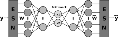
Figure 1: Schematic plot of the ESN-coupled autoencoder.

So far, the presented algorithms measure how good the reconstruction between the original weight $w$ and the reconstructed weights $\tilde{\mbox{\boldmath$w$}}$ is in terms of their $L_{2}$ distance. A better measure would be to check how well the reconstruction $\tilde{\mbox{\boldmath$w$}}$ still represents its corresponding sequence $y$. This can be simply checked by looking at the reconstruction error $\|\mbox{\boldmath$y$}-\mbox{\boldmath$\Phi$}\tilde{\mbox{\boldmath$w$}}\|^{2}$ measured with respect to the sequence $y$, as proposed in Gianniotis et al. (2015). This measure is much more meaningful as it measures reconstruction in terms of the prediction quality of the underlying ESN model. This suggests modifying the reconstruction error of the autoencoder so that it now reads:

$$\|\mbox{\boldmath$y$}-\mbox{\boldmath$\Phi$}f(\mbox{\boldmath$w$};\mbox{\boldmath$\theta$})\|^{2}=\|\mbox{\boldmath$y$}-\mbox{\boldmath$\Phi$}\tilde{\mbox{\boldmath$w$}}\|^{2}=\|\mbox{\boldmath$y$}-\tilde{\mbox{\boldmath$y$}}\|^{2}$$

Essentially, the above reconstruction error entails an autoencoder that is coupled to an ESN as illustrated in Fig. 1: the echo state network is used to encode light curves $y$ as readouts $w$. Next, the readouts are compressed to a low dimensional representation $x$. Out of the low dimensional representation we then reconstruct a readout $\tilde{\mbox{\boldmath$w$}}$ which when plugged back to the ESN should give a reconstruction $\tilde{\mbox{\boldmath$y$}}$ for the input sequence $y$. Optimisation of the autoencoder follows by gradient optimisation via the backpropagation algorithm (Bishop, 1996) as typically done for neural networks. We term the proposed visualisation approach as the ESN-coupled autoencoder which we abbreviate here as ESN-AE.

2.4 Summary of employed models

We briefly summarise the concepts presented in the preceding sections. The basic idea of the presented approach is to find a suitable vector representation of the time series data. Therefore, an ESN is trained on each light curve $y$ and the resulting readout $w$ is used as a fixed-length vector representation.

The standard way of reducing the dimensionality of vectors is to find representations that minimise the $L_{2}$ norm between the original vectors and their reconstructions. This can be done either in a linear (PCA) or non-linear (autoencoder) fashion. However, minimising $\|\mbox{\boldmath$w$}-\tilde{\mbox{\boldmath$w$}}\|^{2}$ is problematic as it does not capture in any way how well the reconstructed readout $\tilde{\mbox{\boldmath$w$}}$ still represents the corresponding light curve $y$. On the other hand, in the proposed ESN-AE model we put forward an alternative reconstruction that measures how well a reconstructed readout weight $\tilde{\mbox{\boldmath$w$}}$ can still predict the original light curves $y$ it represents. In order to distinguish the ESN-AE model from the autoencoder, we henceforth call the later one “plain autoencoder”. We summarise these concepts in Tab. 1.

Visualisation	Linear	Objective
PCA	Yes	$\|\mbox{\boldmath$w$}-\tilde{\mbox{\boldmath$w$}}\|^{2}=\|\mbox{\boldmath$w$}-\mbox{\boldmath$U$}\mbox{\boldmath$U$}^{T}\mbox{\boldmath$w$}\|^{2}$
Plain autoencoder	No	$\|\mbox{\boldmath$w$}-\tilde{\mbox{\boldmath$w$}}\|^{2}=\|\mbox{\boldmath$w$}-f(\mbox{\boldmath$w$};\mbox{\boldmath$\theta$})\|^{2}\$
ESN-AE	No	$\|\mbox{\boldmath$y$}\,-\,\,\tilde{\mbox{\boldmath$y$}}\|^{2}=\|\mbox{\boldmath$y$}\,-\mbox{\boldmath$\Phi$}f(\mbox{\boldmath$w$};\mbox{\boldmath$\theta$})\|^{2}$

Table 1: Summary of proposed visualisation algorithms.

3 Data

The data used in this work come from the Kepler satellite mission described in detail in Borucki et al. (2010). The Kepler mission aims for the detection of Earth-like planets and therefore continuously monitors $150,000$ main sequence stars in a fixed $115$ square degrees field of view located between Cygnus and Lyrae. Besides the detection of exoplanets, the mission opened the window to a detailed study of the dynamical behaviour of variable stars (e.g., RR Lyrae stars). Sources were observed with different cadences over several quarters. In this work, we focus only on data from the first quarter with long exposures of 29.4 min each (33.16 days in total). The available data volume, even in the chosen subset, is quite large as the first quarter comprises already $240$ million photometric measurements. In order to save computing time and focus on objects that have not been classified before, we limit ourselves to objects that are unlikely to be periodic by choosing only objects with $Pf1>0.5$ from the catalogue in Debosscher et al. (2011). In order to include only objects that show considerable variability we select objects with

$$std(F)>3\langle\Delta F\rangle$$

where $F$ is the pre-search data conditioning simple aperture photometry (PDCSAP, Smith et al., 2012) flux of the object and $\langle\Delta F\rangle$ is the average photometric error. The light curves were then preprocessed by taking the logarithm (base 10) of the flux and subtracting the median of it. In order to get rid of individual spikes, caused by cosmic ray hits, we go through the values $y_{t}$ of each light curve and replace them, using a rather conservative constraint, according to:

$$y_{t}=\left\{\begin{array}[]{ll}y_{t}^{repl},\!\!\!\!\!&\mbox{if $(|y_{t-1}-y_{t}|>MAD)\mathrm{\land}(|y_{t+1}-y_{t}|>MAD)$}\\ y_{t},&\mbox{otherwise}\end{array}\right.$$

where

$$y_{t}^{repl}=median(\{y_{t+j}|j\in[-10,10]\})$$

and $MAD$ is the median absolute deviation for the entire light curve $y$. On average, 150 of the 1624 observations have been replaced per time series. After the replacement of spikes, three further light curves had to be excluded: KIC4902072 appears to exceed the numerical range and therefore its amplitude is occasionally swapping signs; KIC4346303 shows dramatically higher amplitude and was removed in order to avoid introducing a bias in the visualisation; KIC6117602 still shows some heavy spikes after the spike removal which are probably of an instrumental origin (damaged pixel) as well. Hence, the final dataset was composed of 6,206 Kepler light curves.

4 Results

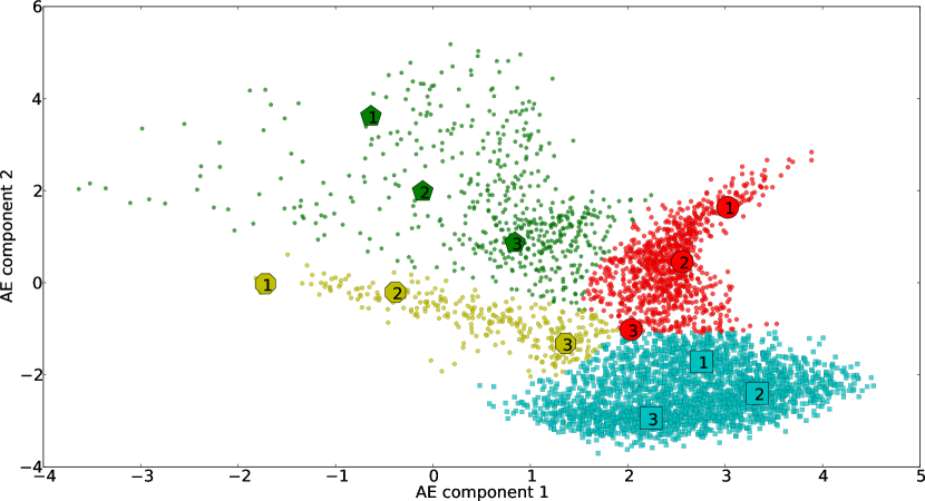
(a) ESN-AE.

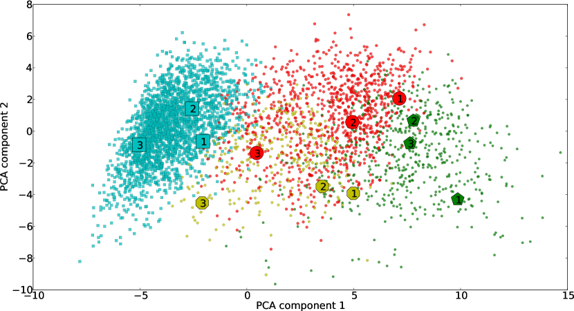
(b) PCA on ESN weights.

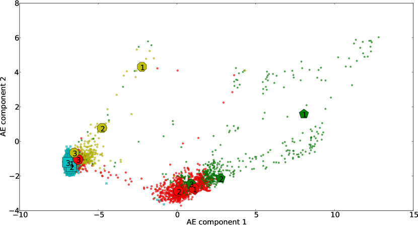
(c) Plain autoencoder on ESN weights.

Figure 2: Visualisation of Kepler light curves using a coupled autoencoder (a), a principal components analysis (b) and a plain autoencoder (c). The visualisations are performed on the weights originating from the ESN. The division into the classes is based on the ESN-AE visualisation. For the sake of clarity, only 60% of the points are plotted.

In Fig. 2, we display the visualisations obtained by the ESN-AE, PCA and a plain autoencoder. We mention in passing that the parameter configuration used for the proposed method was an ESN with a hidden reservoir of $50$ neurons using the cycle architecture (Rodan & Tiňo, 2012) coupled to an autoencoder with a hidden layer of $10$ neurons. More information on the parameters, can be found in Gianniotis et al. (2015). For the plain autoencoder, we also used a hidden layer of $10$ neurons.

The visualisations in Figs. 2(b), 2(c) are driven by optimising the $L_{2}$ norm on the readout representations which means that what they display is a two-dimensional projection of the readouts $w$. On the other hand, the ESN-AE in Fig. 2(a) is driven by optimising reconstruction on the sequences $y$, and hence what we obtain is a two-dimensional projection of the sequences. Though the readout parameters $w$ do capture important information about their respective sequences, we do not expect in general that their visualisation will impart a meaningful result. In other words, PCA and the plain autoencoder judge two light curves to be similar, if their respective readouts are similar in the $L_{2}$ sense. The ESN, however, judges two sequences to be similar if their corresponding readouts result in similar sequences.

We begin our analysis with the ESN-AE in Fig. 2(a). After inspecting this visualisation we noticed that there are, roughly speaking, four regions of particular patterns which we highlight with four different colours. In every coloured region, we have marked three randomly chosen light curves, which we display in Fig. 3. It turns out that the four regions show distinct variability behaviour. The yellow branch shows periodic, dip-like variability, fairly common for rotating stars, while the cyan curves show a prominent variability on time scales of roughly ten days. The red curves are noisy with small-amplitude and short-term variability, while the green curves show a low-amplitude variability as well but on longer time scales. We note that the red and green class are rather similar in their appearance. We also show how the behaviour of sequences smoothly changes variability regimes as we cross the borders of these four regions. For instance, we note how the yellow sequence (1-2-3) transits from short to long term behaviour as we traverse from the edge of the yellow region towards the border with the blue region. A similar behaviour is observed for the red sequences, as we again traverse this region from sequence (1) towards sequence (3) close to the blue and yellow border. This is of course not accidental, but rather by construction, as the ESN-AE is placing similar dynamical behaviour in similar locations.

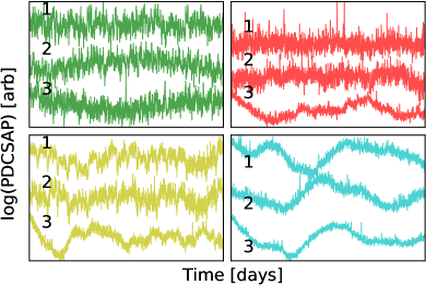
Figure 3: Example light curves drawn from Fig. 2. The x-axis corresponds to 33.16 days for each of the images, ticks have been removed for clarity. The y-axis denotes the logarithm of the PDCSAP flux with an arbitrary offset and scaling for better visibility.

We use the same colours in the other two visualisations, in order to show where each coloured region in Fig. 2(a) is mapped in the PCA visualisation of Fig. 2(b) and in the plain-autoencoder visualisation of Fig. 2(c). We stress at this point that we are aware that our interpretation of the map is subjective, and that other ways of highlighting the visualisation are possible. However, compared to the other visualisations, we find it easier in Fig. 2(a) to discern some structure. For instance, in Fig. 2(b) we see that the readouts $w$ look all rather similar to PCA as no distinct structure stands out. This could be perhaps attributed to the linear and inflexible nature of PCA, as the plain-autoencoder in Fig. 2(c) shows projections organised in certain subgroups.

With the selected example light curves at hand, we are able to reinvestigate the meaning of the visualisations. The transition from short to long term behaviour in the yellow sequence (1-2-3) to the cyan sequences is fairly clear and apparent in all visualisations, even though, the distances are judged quite differently between PCA, ESN-AE on one side and plain autoencoder on the other. Strong support for the ESN-AE and the plain autoencoder comes from the relative distance between red-3 and yellow-3 which is, compared to other distances, quite large in the PCA visualisation. However, when inspecting the light curves we note a strong similarity between these two and attribute the high distance in the PCA to the inflexibility of the visualisation. Two light curves of the green sequence (2,3) show quite significant long-term variability as opposed to the noise-dominated light curves in the red sequence (1,2). In the plain autoencoder, the distances between those are judged significantly different to the PCA and ESN-AE visualisations. While this alone is not a strong argument, it is interesting to see that the noise-dominated light curve from the green sequence (1) is projected very far away from the noisy red ones, in terms of relative distances.

Additionally, the visualisation of the plain autoencoder shows a significant overlap between the yellow, cyan and red light curves, even though, the variability behaviour of these three classes is inherently quite distinct. We also note that the plain autoencoder, does not enjoy the same smooth change in behaviour observed in the ESN-AE visualisation. This is very likely due to the missing link between reconstruction of weights and reconstruction of sequences; this hinders the plain autoencoder in correctly interpreting the weights $w$ leading to a visualisation that cannot be easily comprehended.

Given the above considerations and the principled objective function, we argue that the ESN-AE model provides a better visualisation of the Kepler light curves. Of course, the evaluation of the visualisation is thereby not conclusive. In order to gain further insight as to how meaningful it is, we investigate in the next section how certain physical properties relate to the ESN-AE visualisation.

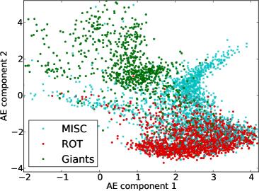
Figure 4: Autoencoder visualisation with overplotted known rotational stars from McQuillan et al. (2014). Additionally, giant stars as obtained by the temperature-$\log g$-criterion in Hekker et al. (2011) are shown. For the sake of clarity, only 60% of the points are plotted.

5 Discussion

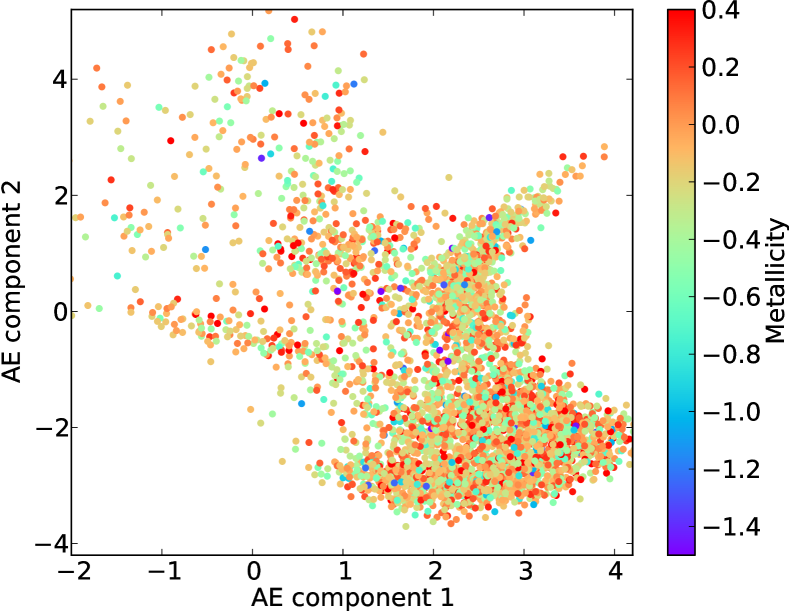
(a) Metallicity

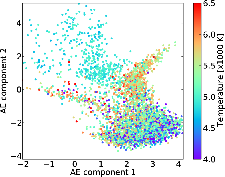
(b) Temperature

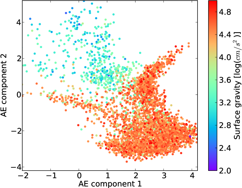
(c) Surface gravity

Figure 5: Visualisation of the coupled autoencoder with overplotted properties from the KIC. A strong correlation between the visualisation and the temperature as well as the surface gravity is apparent. For the sake of clarity, only 60% of the points are plotted. Due to the presence of a few extreme values, we also limit the colour scale to its present range to avoid colour saturation.

The central point of this work is the visualisation of time series with respect to a given model, an ESN in this case. By design, the ESN-AE delivers lower reconstruction errors on time series of all models investigated in the previous section. The other algorithms were only used in order to highlight and discuss the impact of the coupling in the visualisation. Therefore, the discussion focuses solely on the visualisation results of this model.

The periodic variability with dip-like occurrences (yellow region) as well as the long quasi-periodic behaviour of the cyan region are rather typical signs of rotational stars. Fortunately, McQuillan et al. (2014) have scanned the Kepler database for rotationally variable stars. In Fig. 4, the location of the rotational stars found by them and being part of our sample are highlighted in red. One can see that nearly exclusively the cyan and the yellow regions are covered with rotationally variable stars, indicating that many of the stars in these two regions are rotationally variables as well. Therefore, the objects in these classes present high-fidelity candidates for rotational variability as well. It appears that especially the yellow branch contains many formerly undetected objects which show similar dynamical behaviour to the rotating stars. We note that such a clear dependence between the visualisation and the location of the rotational stars is only visible in the ESN-AE visualisation.

While the origin of most of the sources in the cyan and yellow region seems to be resolved, the red and the green regions do not exhibit variability behaviour which could uniquely identify their origin. Therefore, we inspected the data provided by Brown et al. (2011) in the Kepler Input Catalog (KIC). There, stellar model atmospheres (Castelli & Kurucz, 2004) were employed to photometric measurements of the Kepler sources in a probabilistic way. The obtained temperature is uncertain to $\pm 200$ K and the estimate of the logarithm of the surface gravity is uncertain to $0.4\,dex$. With those properties at hand, we highlight the giant stars in our sample, using the temperature-$\log g$-criterion by Hekker et al. (2011). 5969 of the visualised stars have a valid temperature and a valid $\log g$, of which 13% (777) are giants. The giant stars are overplotted in green in Fig. 4 as well. We note that they nearly exclusively populate the green region and are well separated from the remaining main sequence stars.

In Fig. 5, the individual properties from the KIC catalogue are overplotted for the visualised light curves. It is apparent (Fig. 5(a)) that our visualisation does not correlate with metallicity. On the other hand, it has been noted in Brown et al. (2011) that the uncertainty of this estimate is rather high. In contrast to that, a clear correlation between our visualisation and the temperature exists. Nearly all stars have temperatures between 4,000 and 6,000 K (F- and G-type), but in Fig. 5(b) a clear absence of hot or cold stars in the green region is apparent. Additionally, it seems that the hot stars are mainly located in the red and yellow branch, while cold stars can nearly exclusively be found in the bottom part of the cyan region. It should be noted, that the uncertainty in the temperature estimation is not sufficient to explain this separate behaviour. Further support for the visualisation comes from the distribution of surface gravities in Fig. 5(c) which reflects that nearly all giants are located in the green region. The correlation between variability behaviour and stellar properties, such as the surface gravity, has also been studied in Bastien et al. (2013). There, a correlation between the variability - that remains after subtracting the average brightness in 8 hour bins - and the surface gravity was discovered. In Huber et al. (2010), red giant variability was detected by investigating the correlation between frequency separation and the frequency of maximum power. In both publications, the goal was to detect giant stars based on their variability behaviour. To that end, explicit physical knowledge was invoked. It is therefore very pleasing to see that the proposed unsupervised method can also separate the giants based on their variability alone, without any knowledge about periodicity or other physical properties.

So far, this work considered only the unsupervised task of dimensionality reduction of astronomical time series. However, it is possible to extend it to supervised tasks such as classification or regression. We briefly make an example on classifying the giants previously identified in the visualisation. We trained two classifiers. The first one is a random forest trained on all $29$ features in the catalogue by Debosscher et al. (2011) yielding an accuracy of $96.0\pm 0.4\%$. The second one is also a random forest trained on the two visualisation components as inputs yielding a higher classification accuracy of $96.6\pm 0.2\%$. While we emphasise that this is not a conclusive statement on its own, it is remarkable to see that the classification on just the two visualised components performs as well as the one on the $29$ (physically motivated) features. The two visualisation components describe similarity in terms of the dynamical behaviour and appear to be highly informative. In addition, one can consider utilising the ESN readout weights $w$ as features. These can then be used as inputs to a classifier with an objective (cross entropy) function that quantifies classification accuracy rather than reconstruction error.

6 Conclusions

In this work, a new approach to visualise regularly sampled time series was presented. As opposed to visualisation algorithms in astronomy, the presented one does not require any pre-alignment of the data and respects the sequential nature of the time series. Besides that, it is capable to deliver a shift invariant vector representation for sequential data of variable length. Compared to the common use of visualisation algorithms in astronomy, we do not employ the dimensionality reduction directly on the data, but on model parameters instead. We strongly advocate the use of sequential models to describe time series in astronomy and highlight the advantages of those using an ESN. The proposed ESN model returns a fixed-length vector representation for a given sequence. This in turn can then be fed to a visualisation algorithm. In order to enhance the meaning of the visualisation, we measure the reconstruction error not in terms of reconstructing the model parameters but by measuring the direct implications on the reconstruction of the original light curves. This approach provides a powerful objective function which also leads to a more meaningful visualisation.

The proposed visualisation was demonstrated on a selected subset of $6,206$ light curves of variable stars. We studied the quality of the plain and ESN-AE algorithms empirically and concluded that the proposed coupled visualisation algorithm returns results that are easier to interpret. Further support for the proposed visualisation comes from the physical properties of the stars that have been derived from the time series data. With those, we can clearly see that the green cluster is mainly made up from giants with surface temperatures of $5,000-5,500$ K and a significantly lower surface gravity than the main sequence stars in the sample. Besides that, it appears that also separate regions are populated by hot ($>5,500$ K) and cold stars ($<5,500$ K). It is interesting that these physical properties (surface gravity, temperature) show up in the visualisation the way they do, as the underlying model is not aware of them. The correlation between physical properties and variability has been identified in other works by explicitly looking for it using tailored features. The proposed visualisation confirms this correlation thus showing that these physical properties are inherent in the light curve dynamics. We speculate that the ESN readout representation could be further used in regression (e.g. predict surface gravity) and classification (e.g. main sequence versus giant stars) tasks.

The presented approach is modular in the sense that parts of it can be simply replaced. The autoencoder is merely a convenient candidate but other visualisation algorithms could be used instead, perhaps with more favourable computational properties. Additionally, the underlying dynamical ESN model, could be replaced by other models capable of describing sequential data, such as auto-regressive models (ARMA). Finally, the approach is not limited to sequences and in principle other types of astronomical data, given a suitable model, can be visualised in the same fashion. Currently, the visualisation of SDSS spectra using a blackbody model is investigated.

References

- Auvergne et al. (2009) Auvergne M., Bodin P., Boisnard L., et al., 2009, A&A, 506, 411
- Bastien et al. (2013) Bastien F. A., Stassun K. G., Basri G., Pepper J., 2013, Nature, 500, 427
- Benko et al. (2010) Benko J. M., Kolenberg K., Szabó R., et al., 2010, MNRAS, 409, 1585
- Bishop (1996) Bishop C. M., 1996, Neural Networks for Pattern Recognition. Oxford University Press
- Borucki et al. (2010) Borucki W. J., Koch D., Basri G., et al., 2010, Science, 327, 977
- Brown et al. (2011) Brown T. M., Latham D. W., Everett M. E., Esquerdo G. A., 2011, AJ, 142, 112
- Castelli & Kurucz (2004) Castelli F., Kurucz R. L., 2004, ArXiv Astrophysics e-prints
- Debosscher et al. (2011) Debosscher J., Blomme J., Aerts C., De Ridder J., 2011, A&A, 529, A89
- Gianniotis et al. (2015) Gianniotis N., Kügler D., Tino P., Polsterer K., Misra R., 2015, in ESANN Proceedings ’Autoencoding Time Series for Visualisation’. pp 495–500
- Gilliland et al. (2010) Gilliland R. L., Brown T. M., Christensen-Dalsgaard J., et al., 2010, PASP, 122, 131
- Hekker et al. (2011) Hekker S., Gilliland R. L., Elsworth Y., Chaplin W. J., De Ridder J., Stello D., Kallinger T., Ibrahim K. A., Klaus T. C., Li J., 2011, MNRAS, 414, 2594
- Hotelling (1933) Hotelling H., 1933, Journal of Educational Psychology, 24, 417
- Huber et al. (2010) Huber D., Bedding T. R., Stello D., et al., 2010, ApJ, 723, 1607
- Kramer (1991) Kramer M. A., 1991, AICHE Journal, 37, 233
- Kramer et al. (2013) Kramer O., Gieseke F., Polsterer K. L., 2013, Expert Syst. Appl., 40, 2841
- Lissauer et al. (2012) Lissauer J. J., Marcy G. W., Rowe J. F., et al., 2012, ApJ, 750, 112
- Lukosevicius & Jaeger (2009) Lukosevicius M., Jaeger H., 2009, Computer Science Review, 3, 127
- Matijevič et al. (2012) Matijevič G., Prša A., Orosz J. A., et al., 2012, AJ, 143, 123
- McQuillan et al. (2014) McQuillan A., Mazeh T., Aigrain S., 2014, ApJS, 211, 24
- Rodan & Tiňo (2012) Rodan A., Tiňo P., 2012, Neural Computation, 24, 1822
- Slawson et al. (2011) Slawson R. W., Prša A., Welsh W. F., et al., 2011, AJ, 142, 160
- Smith et al. (2012) Smith J. C., Stumpe M. C., Van Cleve J. E., Jenkins J. M., Barclay T. S., Fanelli M. N., Girouard F. R., Kolodziejczak J. J., McCauliff S. D., Morris R. L., Twicken J. D., 2012, PASP, 124, 1000