A globally convergent and locally quadratically
convergent modified B-semismooth Newton method for $\ell_{1}$-penalized minimization

Abstract

We consider the efficient minimization of a nonlinear, strictly convex functional with $\ell_{1}$-penalty term. Such minimization problems appear in a wide range of applications like Tikhonov regularization of (non)linear inverse problems with sparsity constraints. In (2015 Inverse Problems 31 025005), a globalized Bouligand-semismooth Newton method was presented for $\ell_{1}$-Tikhonov regularization of linear inverse problems. Nevertheless, a technical assumption on the accumulation point of the sequence of iterates was necessary to prove global convergence. Here, we generalize this method to general nonlinear problems and present a modified semismooth Newton method for which global convergence is proven without any additional requirements. Moreover, under a technical assumption, full Newton steps are eventually accepted and locally quadratic convergence is achieved. Numerical examples from image deblurring and robust regression demonstrate the performance of the method.
Keywords: global convergence, semismooth Newton method, $\ell_{1}$-Tikhonov regularization, inverse problems, sparsity constraints, quadratic convergence
Mathematics Subject Classification: 49M15, 49N45, 90C56

1 Introduction

We are concerned with the efficient minimization of

$$\min_{\mathbf{u}\in\ell_{2}}g(\mathbf{u})+\sum\limits_{k=1}^{\infty}w_{k}|u_{k}|,$$ (1)

where $g\colon\ell_{2}\to\mathbb{R}$ is a twice Lipschitz-continuously differentiable and strictly convex functional, $\ell_{2}=\ell_{2}(\mathbb{N})$ and $\mathbf{w}=(w_{k})_{k}$ is a positive weight sequence with $w_{k}\geq w_{0}>0$. Minimization problems of the form (1) appear in various applications from engineering and natural sciences. A well-known example is Tikhonov regularization for inverse problems with sparsity constraints, e.g. medical imaging, geophysics, nondestructive testing or compressed sensing, see e.g. [16, 20, 26, 55]. Here, one aims to solve a possibly nonlinear ill-posed operator equation $K(\mathbf{u})=\mathbf{f}$, $K\colon\ell_{2}\to\ell_{2}$. In practice, one has to reconstruct $\mathbf{u}\in\ell_{2}$ from noisy measurement data $\mathbf{f}^{\delta}\approx\mathbf{f}$. In the presence of perturbed data, regularization strategies are required for the stable computation of a numerical solution to an inverse problem [16, 49]. Applying Tikhonov regularization with sparsity constraints, one minimizes a functional consisting of a suitable discrepancy term $g\colon\ell_{2}\to\mathbb{R}$ and a sparsity promoting penalty term, see e.g. [13] and the references therein. Sparsity here means the a priori assumption that the unknown solution is sparse, i.e. $\mathbf{u}$ has only few nonzero entries. As an example, in the special case of a linear discrete ill-posed operator equation $K\mathbf{u}=\mathbf{f}$, $K\colon\ell_{2}\to\ell_{2}$ linear, bounded and injective, $\mathbf{f}\in\ell_{2}$, one may choose the discrepancy term $g(\mathbf{u}):=\frac{1}{2}\|K\mathbf{u}-\mathbf{f}\|_{\ell_{2}}^{2}$ [16]. For nonlinear inverse problems like parameter identification problems, convex discrepancy terms from energy functional approaches may be considered, see e.g. [31, 35, 38, 40]. Sparsity of the Tikhonov minimizer with respect to a given basis can be enforced by using the penalty term in (1), where the weights $w_{k}$ act as regularization parameters, see e.g. [25, 26, 34] and the references therein.

In current research, sparsity-promoting regularization techniques are widely used, see e.g. [6, 13, 24, 26, 33, 34, 38, 39, 40] and the references therein. Such recovery schemes usually outperform classical Tikhonov regularization with $\ell_{2}$ coefficient penalties in terms of reconstruction quality if the unknown solution is sparse w.r.t. some basis. This is the case in many parameter identification problems for partial differential equations with piecewise smooth solutions, like electrical impedance tomography [24, 33] or inverse heat conduction scenarios [7].

There exists a variety of approaches for the numerical minimization of (1) in the literature. In the special case of a quadratic functional $g$, iterative soft-thresholding [13] as well as related approaches for general functionals $g$ are well-studied, see e.g. [6, 8, 48]. Accelerated methods and gradient-based methods introduced in [4, 20, 38, 41, 54] often gain from clever stepsize choices. Homotopy-type solvers [42] and alternating direction methods of multipliers [55] besides many others are also state-of-the-art.

Other popular approaches for the solution of (1) are semismooth Newton methods [9, 52]. A semismooth Newton method and a quasi-Newton method for the minimization of (1) were proposed by Muoi et al. in the infinite-dimensional setting [40], inspired by previous work of Herzog and Lorenz [26]. If $g$ is convex and smooth, it was shown e.g. in [11, 26, 39], that $\mathbf{u}^{*}\in\ell_{2}$ is a minimizer of (1) if and only if $\mathbf{u}^{*}$ is a solution to the zero-finding problem $\mathbf{F}\colon\mathbb{\ell}_{2}\to\ell_{2}$,

$$\mathbf{F}(\mathbf{u}):=\mathbf{u}-\mathbf{S}_{\gamma\mathbf{w}}(\mathbf{u}-\gamma\nabla g(\mathbf{u}))=\mathbf{0}$$ (2)

for any fixed $\gamma>0$, where $\mathbf{S}_{\boldsymbol{\beta}}(\mathbf{u}):=(\operatorname{sgn}(u_{k})(|u_{k}|-\beta_{k})_{+})_{k}$ denotes the componentwise soft thresholding of $\mathbf{u}$ with respect to a positive weight sequence $\boldsymbol{\beta}=(\beta_{k})_{k}$, $\nabla g$ denotes the gradient of $g$ and $x_{+}=\max\{x,0\}$. In [40], $\mathbf{F}$ from (2) was shown to be Newton differentiable, i.e. under a suitable assumption on $g$ there exists a family of slanting functions $\mathbf{G}\colon\ell_{2}\to L(\ell_{2},\ell_{2})$ with

$$\lim\limits_{\mathbf{h}\to\mathbf{0}}\frac{\|\mathbf{F}(\mathbf{u}+\mathbf{h})-\mathbf{F}(\mathbf{u})-\mathbf{G}(\mathbf{u}+\mathbf{h})\mathbf{h}\|_{\ell_{2}}}{\|\mathbf{h}\|_{\ell_{2}}}=0,$$ (3)

see also [9, 26, 52] for the definition of Newton derivatives. A local semismooth Newton method was defined in [40] by

$$\mathbf{G}(\mathbf{u}^{(j)})\mathbf{d}^{(j)} =-\mathbf{F}(\mathbf{u}^{(j)}),$$ (4)

$$\mathbf{u}^{(j+1)} =\mathbf{u}^{(j)}+\mathbf{d}^{(j)},\quad j=0,1,\ldots.$$ (5)

with a specially chosen $\mathbf{G}$, cf. [9, 52]. In [40], locally superlinear convergence was proven under suitable assumptions on the functional $g$.

Nevertheless, the above mentioned semismooth Newton methods are only locally convergent in general. In [39], a semismooth Newton method with filter globalization was presented where semismooth Newton steps are combined with damped shrinkage steps. Another globalized semismooth Newton method was developed in [28]. In loc. cit., inspired by [27, 32, 43, 45], the method from [26] was globalized in a finite-dimensional setting for the special case of a quadratic discrepancy term

$$\min\limits_{\mathbf{u}\in\mathbb{R}^{n}}\frac{1}{2}\|\mathbf{K}\mathbf{u}-\mathbf{f}\|_{2}^{2}+\sum\limits_{k=1}^{n}w_{k}|u_{k}|,$$ (6)

where $\mathbf{K}\in\mathbb{R}^{m\times n}$ is injective and $\mathbf{f}\in\mathbb{R}^{m}$. In [28], $\mathbf{F}$ was shown to be Lipschitz continuous and directionally differentiable, i.e. Bouligand differentiable [17, 43, 50]. For such nonlinearities a B(ouligand)-Newton method can be defined [43], replacing (4) by the generalized Newton equation

$$\mathbf{F}^{\prime}(\mathbf{u}^{(j)},\mathbf{d}^{(j)})=-\mathbf{F}(\mathbf{u}^{(j)}).$$ (7)

In [28], the system (7) was shown to be equivalent to a uniquely solvable mixed linear complementarity problem [12]. By the choice (7), $\mathbf{d}^{(j)}$ automatically is a descent direction with respect to the merit functional $\Theta\colon\mathbb{R}^{n}\to\mathbb{R}$,

$$\Theta(\mathbf{u}):=\|\mathbf{F}(\mathbf{u})\|_{2}^{2},$$ (8)

cf. [43]. Additionally, this Bouligand-Newton method can be interpreted as a semismooth Newton method with a specially chosen slanting function and is therefore called a B-semismooth Newton method, cf. [46]. By introducing suitable damping parameters, the method can be shown to be globally convergent under a technical assumption on the in practice unknown accumulation point $\mathbf{u}^{*}$ of the sequence of iterates, see also [27, 32, 43, 45]. Indeed, if the chosen Armijo stepsizes tend to zero, the merit functional $\Theta$ has to fulfill the condition

$$\lim\limits_{(\mathbf{u},\mathbf{v})\to(\mathbf{u}^{*},\mathbf{u}^{*})}\frac{\Theta(\mathbf{u})-\Theta(\mathbf{v})-\Theta^{\prime}(\mathbf{u}^{*},\mathbf{u}-\mathbf{v})}{\|\mathbf{u}-\mathbf{v}\|_{2}}=0$$ (9)

at $\mathbf{u}^{*}$ to ensure global convergence.

In this work, we present a modified, globally convergent semismooth Newton method for the minimization problem (1) in the finite-dimensional setting

$$\min\limits_{\mathbf{u}\in\mathbb{R}^{n}}g(\mathbf{u})+\sum\limits_{k=1}^{n}w_{k}|u_{k}|$$ (10)

for general (not necessarily quadratic) strictly convex functionals $g\colon\mathbb{R}^{n}\to\mathbb{R}$. Our work is inspired by Pang [44], where a globally and locally quadratically convergent modified Bouligand-Newton method was presented for the solution of variational inequalities, nonlinear complementarity problems and nonlinear programs. We take advantage of similarities of nonlinear complementarity problems and the zero-finding problem (2) to propose a modified method similar to [44]. Starting out from [28, 40], we develop a globalized B-semismooth Newton method for general possibly nonquadratic discrepancy functionals $g$. In order to achieve global convergence without any requirements on the a priori unknown accumulation point of the iterates, inspired by [44], we propose a special modification of the Newton directions $\mathbf{d}^{(j)}$ from (7), retaining the descent property w.r.t. $\Theta$. The resulting generalized Newton equation is again shown to be equivalent to a uniquely solvable mixed linear complementarity problem. Fortunately, in our proposed scheme, under a technical assumption, full Newton steps are accepted in the vicinity of the zero of $\mathbf{F}$. As a consequence, under an additional regularity assumption, locally quadratic convergence is achieved. Additionally, the resulting modified method can be interpreted as a generalized Newton method proposed by Han, Pang and Rangaraj [27]. In a neighborhood of the zero of $\mathbf{F}$, the modified method, under a technical assumption, coincides with the B-semismooth Newton method from [28] reformulated for nonquadratic $g$. If $g$ is a quadratic functional, it was shown in [28] that in a neighborhood of the zero, the B-semismooth Newton method finds the exact zero of $\mathbf{F}$ within finitely many iterations.

Alternatively, one may consider other globalization strategies as trust region methods or path-search methods instead of the considered line-search damping strategy, see e.g. [52, 18] and the references therein. The path-search globalization strategy proposed by the authors of [47, 14] could be a promising, albeit conceptually different, alternative. These approaches go beyond the scope of this paper and are part of future work.

For the rest of the paper, we require the following assumption on the smoothness of $g$, similar to [40, Assumption 3.1, Example 3.4]. In Section 3, we will need a further assumption regarding the locally quadratic convergence of the method.

Assumption 1.

1. The function $g$ is twice Lipschitz-continuously differentiable and the Hessian $\nabla^{2}g(\mathbf{u})$ is positive definite for all $\mathbf{u}\in\mathbb{R}^{n}$. Moreover, there exist constants $0<c_{1},c_{2}<\infty$ with

   $$c_{1}\|\mathbf{h}\|_{2}^{2}\leq\langle\nabla^{2}g(\mathbf{u})\mathbf{h},\mathbf{h}\rangle\leq c_{2}\|\mathbf{h}\|_{2}^{2},\qquad\text{for all }\mathbf{h}\in\mathbb{R}^{n},$$

   uniformly for all $\mathbf{u}\in\mathbb{R}^{n}$.

2. The level sets $L_{\Theta}(\mathbf{u}^{(0)}):=\{\mathbf{u}\in\mathbb{R}^{n}:\Theta(\mathbf{u})\leq\Theta(\mathbf{u}^{(0)})\}$ of $\Theta$ are compact.

The compactness of the level sets in the case of a quadratic functional $g(\mathbf{u})=\frac{1}{2}\|\mathbf{K}\mathbf{u}-\mathbf{f}\|_{2}^{2}$, $\mathbf{K}\in\mathbb{R}^{m\times n}$ injective, $n\leq m$, $\mathbf{f}\in\mathbb{R}^{m}$ was shown in [28]. Note that the positive definiteness of the Hessian $\nabla^{2}g(\mathbf{u})$ implies strict convexity of the functional $g$ and ensures unique solvability of (10).

The paper is organized as follows. Section 2 treats the proposed B-semismooth Newton method and its modification as well as their feasibility. Section 3 addresses the global convergence and the local convergence speed of the methods. Numerical examples demonstrate the performance of the proposed algorithms in Section 4.

2 A B-semismooth Newton method and its modification

In this section, we present the algorithm of the B-semismooth Newton method from [28] generalized to the minimization problem (10) as well as a modified version and discuss their feasibility. Additionally, we suggest a hybrid method. We start with the modified algorithm because the generalized B-semismooth Newton method can immediately be deduced from the modified method.

2.1 A modified B-semismooth Newton method and its feasibility

In the following, we introduce a modified B-semismooth Newton method for the solution of (10). We denote the active set by $\mathcal{A}(\mathbf{u}):=\mathcal{A}^{+}(\mathbf{u})\cup\mathcal{A}^{-}(\mathbf{u})$, where

$$\mathcal{A}^{+}(\mathbf{u}) :=\{k:\gamma(\nabla g(\mathbf{u}))_{k}+\gamma w_{k}<u_{k}\},$$ (11)

$$\mathcal{A}^{-}(\mathbf{u}) :=\{k:u_{k}<\gamma(\nabla g(\mathbf{u}))_{k}-\gamma w_{k}\},$$ (12)

and the inactive set by $\mathcal{I}(\mathbf{u}):=\mathcal{I}^{\circ}(\mathbf{u})\cup\mathcal{I}^{+}(\mathbf{u})\cup\mathcal{I}^{-}(\mathbf{u})$, where

$$\mathcal{I}^{\circ}(\mathbf{u}) :=\{k:\gamma(\nabla g(\mathbf{u}))_{k}-\gamma w_{k}<u_{k}<\gamma(\nabla g(\mathbf{u}))_{k}+\gamma w_{k}\},$$ (13)

$$\mathcal{I}^{+}(\mathbf{u}) :=\{k:u_{k}=\gamma(\nabla g(\mathbf{u}))_{k}+\gamma w_{k}\},$$ (14)

$$\mathcal{I}^{-}(\mathbf{u}) :=\{k:u_{k}=\gamma(\nabla g(\mathbf{u}))_{k}-\gamma w_{k}\}.$$ (15)

Below, we drop the argument $\mathbf{u}$ if there is no risk of confusion.

For $\mathbf{F}\colon\mathbb{R}^{n}\to\mathbb{R}^{n}$ defined by (2), we then have

$$F_{k}(\mathbf{u}) =\min\{\gamma(\nabla g(\mathbf{u}))_{k}+\gamma w_{k},u_{k}\}, k\in\mathcal{A}^{+}(\mathbf{u})\cup\mathcal{I}^{\circ}(\mathbf{u})\cup\mathcal{I}^{+}(\mathbf{u}),$$ (16)

$$F_{k}(\mathbf{u}) =\max\{\gamma(\nabla g(\mathbf{u}))_{k}-\gamma w_{k},u_{k}\}, k\in\mathcal{A}^{-}(\mathbf{u})\cup\mathcal{I}^{\circ}(\mathbf{u})\cup\mathcal{I}^{-}(\mathbf{u}).$$ (17)

By Assumption 1, $\mathbf{F}$ is Lipschitz continuous and directionally differentiable. The directional derivative of $\mathbf{F}$ can be easily deduced.

Lemma 2.

The directional derivative of $\mathbf{F}$ at $\mathbf{u}\in\mathbb{R}^{n}$ in the direction $\mathbf{d}\in\mathbb{R}^{n}$ is given elementwise by

$$F^{\prime}_{k}(\mathbf{u},\mathbf{d})=\begin{cases}\gamma(\nabla^{2}g(\mathbf{u})\mathbf{d})_{k},&k\in\mathcal{A}(\mathbf{u}),\\ d_{k},&k\in\mathcal{I}^{\circ}(\mathbf{u}),\\ \min\{\gamma(\nabla^{2}g(\mathbf{u})\mathbf{d})_{k},d_{k}\},&k\in\mathcal{I}^{+}(\mathbf{u}),\\ \max\{\gamma(\nabla^{2}g(\mathbf{u})\mathbf{d})_{k},d_{k}\},&k\in\mathcal{I}^{-}(\mathbf{u}).\end{cases}$$ (18)

Proof.

The claim is trivially true for $k\in\mathcal{A}(\mathbf{u})$ and $k\in\mathcal{I}^{\circ}(\mathbf{u})$. For $k\in\mathcal{I}^{+}(\mathbf{u})$ we have with (14) and (16)

$$\lim\limits_{t\searrow 0}\frac{\min\{\gamma(\nabla g(\mathbf{u}+t\mathbf{d}))_{k}+\gamma w_{k},u_{k}+td_{k}\}-\min\{\gamma(\nabla g(\mathbf{u}))_{k}+\gamma w_{k},u_{k}\}}{t}$$

$$= \lim\limits_{t\searrow 0}\frac{\min\{\gamma(\nabla g(\mathbf{u}+t\mathbf{d}))_{k}-\gamma(\nabla g(\mathbf{u}))_{k},td_{k}\}}{t}$$

$$= \min\Big{\{}\lim\limits_{t\searrow 0}\frac{\gamma(\nabla g(\mathbf{u}+t\mathbf{d}))_{k}-\gamma(\nabla g(\mathbf{u}))_{k}}{t},d_{k}\Big{\}}$$

$$= \min\{\gamma(\nabla^{2}g(\mathbf{u})\mathbf{d})_{k},d_{k}\}.$$

The claim for $k\in\mathcal{I}^{-}(\mathbf{u})$ results analogously. ∎

The directional derivative of the merit functional $\Theta$ from (8) at $\mathbf{u}\in\mathbb{R}^{n}$ in the direction $\mathbf{d}\in\mathbb{R}^{n}$ is given by $\Theta^{\prime}(\mathbf{u},\mathbf{d})=2\langle\mathbf{F}^{\prime}(\mathbf{u},\mathbf{d}),\mathbf{F}(\mathbf{u})\rangle$, where $\langle\cdot,\cdot\rangle$ denotes the Euclidean scalar product, see e.g. [28, Lemma 3.2].

To introduce the modified semismooth Newton method, we define the subsets

$$\mathcal{A}^{+}_{+}(\mathbf{u}) :=\{k:\gamma(\nabla g(\mathbf{u}))_{k}+\gamma w_{k}<u_{k}<0\},$$ (19)

$$\mathcal{A}^{-}_{-}(\mathbf{u}) :=\{k:0<u_{k}<\gamma(\nabla g(\mathbf{u}))_{k}-\gamma w_{k}\},$$ (20)

$$\mathcal{I}^{\circ}_{+}(\mathbf{u}) :=\{k:\gamma(\nabla g(\mathbf{u}))_{k}-\gamma w_{k}<u_{k}<\gamma(\nabla g(\mathbf{u}))_{k}+\gamma w_{k}<0\},$$ (21)

$$\mathcal{I}^{\circ}_{-}(\mathbf{u}) :=\{k:0<\gamma(\nabla g(\mathbf{u}))_{k}-\gamma w_{k}<u_{k}<\gamma(\nabla g(\mathbf{u}))_{k}+\gamma w_{k}\}.$$ (22)

Inspired by [44], we define the modified index sets

$$\overline{\mathcal{A}^{+}}(\mathbf{u}) :=\mathcal{A}^{+}(\mathbf{u})\setminus\mathcal{A}^{+}_{+}(\mathbf{u}),$$ (23)

$$\overline{\mathcal{A}^{-}}(\mathbf{u}) :=\mathcal{A}^{-}(\mathbf{u})\setminus\mathcal{A}^{-}_{-}(\mathbf{u}),$$ (24)

$$\overline{\mathcal{I}^{\circ}}(\mathbf{u}) :=\mathcal{I}^{\circ}(\mathbf{u})\setminus\big{(}\mathcal{I}^{\circ}_{+}(\mathbf{u})\cup\mathcal{I}^{\circ}_{-}(\mathbf{u})\big{)},$$ (25)

$$\overline{\mathcal{I}^{+}}(\mathbf{u}) :=\mathcal{I}^{+}(\mathbf{u})\cup\mathcal{A}^{+}_{+}(\mathbf{u})\cup\mathcal{I}^{\circ}_{+}(\mathbf{u}),$$ (26)

$$\overline{\mathcal{I}^{-}}(\mathbf{u}) :=\mathcal{I}^{-}(\mathbf{u})\cup\mathcal{A}^{-}_{-}(\mathbf{u})\cup\mathcal{I}^{\circ}_{-}(\mathbf{u}).$$ (27)

We denote $\overline{\mathcal{A}}(\mathbf{u}):=\overline{\mathcal{A}^{+}}(\mathbf{u})\cup\overline{\mathcal{A}^{-}}(\mathbf{u})$ and $\overline{\mathcal{I}}(\mathbf{u}):=\overline{\mathcal{I}^{\circ}}(\mathbf{u})\cup\overline{\mathcal{I}^{+}}(\mathbf{u})\cup\overline{\mathcal{I}^{-}}(\mathbf{u})$ respectively. The subsets (19)–(22) fulfill $\mathcal{A}^{+}_{+}(\mathbf{u})=\emptyset$, $\mathcal{A}^{-}_{-}(\mathbf{u})=\emptyset$, $\mathcal{I}^{\circ}_{+}(\mathbf{u})=\emptyset$ and $\mathcal{I}^{\circ}_{-}(\mathbf{u})=\emptyset$ if $\mathbf{F}(\mathbf{u})=\mathbf{0}$.

In the following lemma, we consider a linear complementarity problem which is important for all further discussions, cf. [28].

Lemma 3.

Let $\mathbf{u}\in\mathbb{R}^{n}$ and $\mathbf{M}:=\nabla^{2}g(\mathbf{u})$. The linear complementarity problem

$$\mathbf{x}\geq\mathbf{0},\quad\mathbf{N}\mathbf{x}+\mathbf{z}\geq\mathbf{0},\quad\langle\mathbf{x},\mathbf{N}\mathbf{x}+\mathbf{z}\rangle=0,$$ (28)

with

$$\mathbf{N}= \mathbf{N}(\mathbf{u})$$

$$:= \gamma\begin{pmatrix}\mathbf{M}_{\overline{\mathcal{I}^{+}},\overline{\mathcal{I}^{+}}}-\mathbf{M}_{\overline{\mathcal{I}^{+}},\overline{\mathcal{A}}}\mathbf{M}_{\overline{\mathcal{A}},\overline{\mathcal{A}}}^{-1}\mathbf{M}_{\overline{\mathcal{A}},\overline{\mathcal{I}^{+}}}&\mathbf{M}_{\overline{\mathcal{I}^{+}},\overline{\mathcal{A}}}\mathbf{M}_{\overline{\mathcal{A}},\overline{\mathcal{A}}}^{-1}\mathbf{M}_{\overline{\mathcal{A}},\overline{\mathcal{I}^{-}}}-\mathbf{M}_{\overline{\mathcal{I}^{+}},\overline{\mathcal{I}^{-}}}\\ \mathbf{M}_{\overline{\mathcal{I}^{-}},\overline{\mathcal{A}}}\mathbf{M}_{\overline{\mathcal{A}},\overline{\mathcal{A}}}^{-1}\mathbf{M}_{\overline{\mathcal{A}},\overline{\mathcal{I}^{+}}}-\mathbf{M}_{\overline{\mathcal{I}^{-}},\overline{\mathcal{I}^{+}}}&\mathbf{M}_{\overline{\mathcal{I}^{-}},\overline{\mathcal{I}^{-}}}-\mathbf{M}_{\overline{\mathcal{I}^{-}},\overline{\mathcal{A}}}\mathbf{M}_{\overline{\mathcal{A}},\overline{\mathcal{A}}}^{-1}\mathbf{M}_{\overline{\mathcal{A}},\overline{\mathcal{I}^{-}}}\end{pmatrix}$$ (29)

and

$$\begin{split}&\mathbf{z}=\mathbf{z}(\mathbf{u})\\ &:=\begin{pmatrix}\gamma(\mathbf{M}_{\overline{\mathcal{I}^{+}},\overline{\mathcal{A}}}\mathbf{M}_{\overline{\mathcal{A}},\overline{\mathcal{A}}}^{-1}\mathbf{M}_{\overline{\mathcal{A}},\overline{\mathcal{I}^{\circ}}}-\mathbf{M}_{\overline{\mathcal{I}^{+}},\overline{\mathcal{I}^{\circ}}})\mathbf{u}_{\overline{\mathcal{I}^{\circ}}}-\mathbf{M}_{\overline{\mathcal{I}^{+}},\overline{\mathcal{A}}}\mathbf{M}_{\overline{\mathcal{A}},\overline{\mathcal{A}}}^{-1}\mathbf{F}(\mathbf{u})_{\overline{\mathcal{A}}}+\mathbf{F}(\mathbf{u})_{\overline{\mathcal{I}^{+}}}\\ \gamma(\mathbf{M}_{\overline{\mathcal{I}^{-}},\overline{\mathcal{I}^{\circ}}}-\mathbf{M}_{\overline{\mathcal{I}^{-}},\overline{\mathcal{A}}}\mathbf{M}_{\overline{\mathcal{A}},\overline{\mathcal{A}}}^{-1}\mathbf{M}_{\overline{\mathcal{A}},\overline{\mathcal{I}^{\circ}}})\mathbf{u}_{\overline{\mathcal{I}^{\circ}}}+\mathbf{M}_{\overline{\mathcal{I}^{-}},\overline{\mathcal{A}}}\mathbf{M}_{\overline{\mathcal{A}},\overline{\mathcal{A}}}^{-1}\mathbf{F}(\mathbf{u})_{\overline{\mathcal{A}}}-\mathbf{F}(\mathbf{u})_{\overline{\mathcal{I}^{-}}}\end{pmatrix}\\ &\phantom{:=}\ -\mathbf{N}(\mathbf{u})\begin{pmatrix}\mathbf{u}_{\overline{\mathcal{I}^{+}}}\\ -\mathbf{u}_{\overline{\mathcal{I}^{-}}}\end{pmatrix}\end{split}$$ (30)

has a unique solution.

Proof.

By Assumption 1, $\mathbf{M}=\nabla^{2}g(\mathbf{u})$ is symmetric and positive definite. Therefore, $\mathbf{N}$ from (3) is symmetric and positive definite, see [28, Lemma 3.3]. Hence (28) is uniquely solvable, see [12, Theorem 3.3.7] and [28, Theorem 3.5]. ∎

Now we can define the generalized Newton equation for $\mathbf{F}$, cf. [28]. Let $\mathbf{u}\in\mathbb{R}^{n}$ and

$$\begin{split}\mathcal{B}&=\mathcal{B}(\mathbf{u}):=\overline{\mathcal{A}}(\mathbf{u})\cup\{k\in\overline{\mathcal{I}^{+}}(\mathbf{u})\cup\overline{\mathcal{I}^{-}}(\mathbf{u}):x_{k}>0\},\\ \mathcal{C}&=\mathcal{C}(\mathbf{u}):=\overline{\mathcal{I}^{\circ}}(\mathbf{u})\cup\{k\in\overline{\mathcal{I}^{+}}(\mathbf{u})\cup\overline{\mathcal{I}^{-}}(\mathbf{u}):x_{k}=0\},\end{split}$$ (31)

where $\mathbf{x}=(x_{k})_{k}$ is the unique solution to the linear complementarity problem (28). Then, by defining the generalized derivative blockwise

$$\begin{pmatrix}\mathbf{G}(\mathbf{u})_{\mathcal{B},\mathcal{B}}&\mathbf{G}(\mathbf{u})_{\mathcal{B},\mathcal{C}}\\ \mathbf{G}(\mathbf{u})_{\mathcal{C},\mathcal{B}}&\mathbf{G}(\mathbf{u})_{\mathcal{C},\mathcal{C}}\end{pmatrix}:=\begin{pmatrix}\gamma(\nabla^{2}g(\mathbf{u}))_{\mathcal{B},\mathcal{B}}&\gamma(\nabla^{2}g(\mathbf{u}))_{\mathcal{B},\mathcal{C}}\\ \mathbf{0}_{\mathcal{C},\mathcal{B}}&\mathbf{I}_{\mathcal{C},\mathcal{C}}\end{pmatrix}\in\mathbb{R}^{n\times n},$$ (32)

the modified semismooth Newton method is given by

$$\mathbf{G}(\mathbf{u}^{(j)})\mathbf{d}^{(j)} =-\mathbf{F}(\mathbf{u}^{(j)}),$$ (33)

$$\mathbf{u}^{(j+1)} =\mathbf{u}^{(j)}+t_{j}\mathbf{d}^{(j)},\quad j=0,1,\ldots$$ (34)

with suitably chosen damping parameters $t_{j}\in(0,1]$.

Remark 4.

In [40], Muoi et al. chose the slanting function

$$\begin{pmatrix}\mathbf{G}(\mathbf{u})_{\mathcal{A},\mathcal{A}}&\mathbf{G}(\mathbf{u})_{\mathcal{A},\mathcal{I}}\\ \mathbf{G}(\mathbf{u})_{\mathcal{I},\mathcal{A}}&\mathbf{G}(\mathbf{u})_{\mathcal{I},\mathcal{I}}\end{pmatrix}=\begin{pmatrix}\gamma(\nabla^{2}g(\mathbf{u}))_{\mathcal{A},\mathcal{A}}&\gamma(\nabla^{2}g(\mathbf{u}))_{\mathcal{A},\mathcal{I}}\\ \mathbf{0}_{\mathcal{I},\mathcal{A}}&\mathbf{I}_{\mathcal{I},\mathcal{I}}\end{pmatrix},$$ (35)

blocked according to the active and inactive sets, to define the local semismooth Newton method (4),(5). The key difference of (32) compared to (35) is the modification of the index sets. Note that $\mathbf{G}$ from (32) is not a slanting function in general because in regions where $\mathbf{F}$ is smooth, $\mathbf{G}$ does not coincide with the Fréchet-derivative of $\mathbf{F}$.

Let $\mathbf{u}^{(j)}\in\mathbb{R}^{n}$ and $\mathbf{M}:=\nabla^{2}g(\mathbf{u}^{(j)})$. Then $\mathbf{d}^{(j)}\in\mathbb{R}^{n}$ solves (33) if and only if

$$\gamma(\mathbf{M}\mathbf{d}^{(j)})_{\overline{\mathcal{A}}} =-\mathbf{F}(\mathbf{u}^{(j)})_{\overline{\mathcal{A}}},$$ (36)

$$\mathbf{d}_{\overline{\mathcal{I}^{\circ}}}^{(j)} =-\mathbf{u}_{\overline{\mathcal{I}^{\circ}}}^{(j)},$$ (37)

and

$$\mathbf{x} :=\begin{pmatrix}\mathbf{d}_{\overline{\mathcal{I}^{+}}}^{(j)}+\mathbf{u}_{\overline{\mathcal{I}^{+}}}^{(j)}\\ -\mathbf{d}_{\overline{\mathcal{I}^{-}}}^{(j)}-\mathbf{u}_{\overline{\mathcal{I}^{-}}}^{(j)}\end{pmatrix}$$ (38)

$$\mathbf{y} :=\mathbf{N}(\mathbf{u}^{(j)})\mathbf{x}+\mathbf{z}(\mathbf{u}^{(j)})=\begin{pmatrix}\gamma(\mathbf{M}\mathbf{d}^{(j)})_{\overline{\mathcal{I}^{+}}}+(\mathbf{F}(\mathbf{u}^{(j)}))_{\overline{\mathcal{I}^{+}}}\\ -\gamma(\mathbf{M}\mathbf{d}^{(j)})_{\overline{\mathcal{I}^{-}}}-(\mathbf{F}(\mathbf{u}^{(j)}))_{\overline{\mathcal{I}^{-}}}\end{pmatrix},$$

where $\mathbf{x}$, $\mathbf{y}$ solve the linear complementarity problem (28), cf. [28, Lemma 3.4].

We summarize the above observations in the following lemma, cf. [28, Theorem 3.5].

Lemma 5.

Let $\mathbf{x}$ be the unique solution to (28) for an iterate $\mathbf{u}^{(j)}\in\mathbb{R}^{n}$ and $\mathbf{M}:=\nabla^{2}g(\mathbf{u}^{(j)})$. Then, the Newton update $\mathbf{d}^{(j)}$ from (33) is given by

$$\mathbf{d}^{(j)}_{\overline{\mathcal{I}^{\circ}}} =-\mathbf{u}^{(j)}_{\overline{\mathcal{I}^{\circ}}},$$ (39)

$$\mathbf{d}^{(j)}_{\overline{\mathcal{I}^{+}}} =\mathbf{x}_{\overline{\mathcal{I}^{+}}}-\mathbf{u}^{(j)}_{\overline{\mathcal{I}^{+}}},$$

$$\mathbf{d}^{(j)}_{\overline{\mathcal{I}^{-}}} =-\mathbf{x}_{\overline{\mathcal{I}^{-}}}-\mathbf{u}^{(j)}_{\overline{\mathcal{I}^{-}}},$$

$$\mathbf{d}^{(j)}_{\overline{\mathcal{A}}} =\frac{1}{\gamma}\mathbf{M}_{\overline{\mathcal{A}},\overline{\mathcal{A}}}^{-1}\big{(}-\gamma\mathbf{M}_{\overline{\mathcal{A}},\overline{\mathcal{I}}}\mathbf{d}^{(j)}_{\overline{\mathcal{I}}}-\mathbf{F}(\mathbf{u}^{(j)})_{\overline{\mathcal{A}}}\big{)}.$$

Before proceeding, we prove some useful identities similar to [44, Lemma 2].

Lemma 6.

Let $\mathbf{u}\in\mathbb{R}^{n}$, $\mathbf{d}=\mathbf{d}(\mathbf{u})$ the unique solution to (39) and $\mathbf{M}=\nabla^{2}g(\mathbf{u})$. For $k\in\{1,\ldots,n\}$, we have the following identities

$$(\gamma(\nabla g(\mathbf{u}))_{k}+\gamma w_{k})\gamma(\mathbf{M}\mathbf{d})_{k} =-(\gamma(\nabla g(\mathbf{u}))_{k}+\gamma w_{k})^{2}, k\in\overline{\mathcal{A}^{+}}(\mathbf{u}),$$ (40)

$$(\gamma(\nabla g(\mathbf{u}))_{k}-\gamma w_{k})\gamma(\mathbf{M}\mathbf{d})_{k} =-(\gamma(\nabla g(\mathbf{u}))_{k}-\gamma w_{k})^{2}, k\in\overline{\mathcal{A}^{-}}(\mathbf{u}),$$ (41)

$$u_{k}d_{k} =-u_{k}^{2}, k\in\overline{\mathcal{I}^{\circ}}(\mathbf{u}).$$ (42)

Additionally, for $k\in\mathcal{A}^{+}_{+}(\mathbf{u})\cup\mathcal{I}^{\circ}_{+}(\mathbf{u})\cup\{k\in\mathcal{I}^{+}(\mathbf{u}):F_{k}(\mathbf{u})<0)\}$ the inequality

$$(\gamma(\nabla g(\mathbf{u}))_{k}+\gamma w_{k})\gamma(\mathbf{M}\mathbf{d})_{k} \leq-(\gamma(\nabla g(\mathbf{u}))_{k}+\gamma w_{k})^{2}$$ (43)

holds, for $k\in\mathcal{A}^{-}_{-}(\mathbf{u})\cup\mathcal{I}^{\circ}_{-}(\mathbf{u})\cup\{k\in\mathcal{I}^{-}(\mathbf{u}):F_{k}(\mathbf{u})>0)\}$ we have

$$(\gamma(\nabla g(\mathbf{u}))_{k}-\gamma w_{k})\gamma(\mathbf{M}\mathbf{d})_{k} \leq-(\gamma(\nabla g(\mathbf{u}))_{k}-\gamma w_{k})^{2}$$ (44)

and for $k\in\mathcal{A}^{+}_{+}(\mathbf{u})\cup\mathcal{A}^{-}_{-}(\mathbf{u})\cup\mathcal{I}^{\circ}_{+}(\mathbf{u})\cup\mathcal{I}^{\circ}_{-}(\mathbf{u})\cup\{k\in\mathcal{I}^{+}(\mathbf{u}):F_{k}(\mathbf{u})<0)\}\cup\{k\in\mathcal{I}^{-}(\mathbf{u}):F_{k}(\mathbf{u})>0)\}$ we have

$$u_{k}d_{k} \leq-u_{k}^{2}.$$ (45)

Proof.

Equations (40), (41) and (42) immediately follow from (36) and (37). For $k\in\mathcal{A}^{+}_{+}(\mathbf{u})\cup\mathcal{I}^{\circ}_{+}(\mathbf{u})\cup\{k\in\mathcal{I}^{+}(\mathbf{u}):F_{k}(\mathbf{u})<0)\}$, we have by definition $\gamma(\nabla g(\mathbf{u}))_{k}+\gamma w_{k}<0$ and with (28) and (38) we have $\gamma(\mathbf{M}\mathbf{d})_{k}\geq-F_{k}(\mathbf{u})\geq-(\gamma(\nabla g(\mathbf{u}))_{k}+\gamma w_{k})$ implying (43). For $k\in\mathcal{A}^{-}_{-}(\mathbf{u})\cup\mathcal{I}^{\circ}_{-}(\mathbf{u})\cup\{k\in\mathcal{I}^{-}(\mathbf{u}):F_{k}(\mathbf{u})>0)\}$, we have by definition $\gamma(\nabla g(\mathbf{u}))_{k}-\gamma w_{k}>0$ and with (28) and (38) we have $\gamma(\mathbf{M}\mathbf{d})_{k}\leq-F_{k}(\mathbf{u})\leq-(\gamma(\nabla g(\mathbf{u}))_{k}-\gamma w_{k})$, implying (44).

For $k\in\mathcal{A}^{+}_{+}(\mathbf{u})\cup\mathcal{I}^{\circ}_{+}(\mathbf{u})\cup\{k\in\mathcal{I}^{+}(\mathbf{u}):F_{k}(\mathbf{u})<0\}$, we have $u_{k}<0$ and $d_{k}\geq-u_{k}$ because of (28) and (38). If $k\in\mathcal{A}^{-}_{-}(\mathbf{u})\cup\mathcal{I}^{\circ}_{-}(\mathbf{u})\cup\{k\in\mathcal{I}^{-}(\mathbf{u}):F_{k}(\mathbf{u})>0\}$, we have $u_{k}>0$ and $d_{k}\leq-u_{k}$ because of (28) and (38). In both cases (45) follows. ∎

Now we verify that $\mathbf{d}=\mathbf{d}(\mathbf{u})$ from (39) is a descent direction of the merit functional $\Theta$ from (8) at $\mathbf{u}$.

Lemma 7.

Let $\mathbf{u}\in\mathbb{R}^{n}$ with $\Theta(\mathbf{u})>0$ and $\mathbf{M}:=\nabla^{2}g(\mathbf{u})$. Let $\mathbf{d}=\mathbf{d}(\mathbf{u})\in\mathbb{R}^{n}$ be the solution to (39). Then, we have

$$\Theta^{\prime}(\mathbf{u},\mathbf{d})\leq-2\Theta(\mathbf{u})<0,$$ (46)

i.e. $\mathbf{d}$ is a true descent direction of $\Theta$ at $\mathbf{u}$ in the direction $\mathbf{d}$.

Proof.

The proof follows the idea of [44, Proof of Proposition 5]. We have

$$\Theta^{\prime}(\mathbf{u},\mathbf{d})=2\langle\mathbf{F}(\mathbf{u}),\mathbf{F}^{\prime}(\mathbf{u},\mathbf{d})\rangle=2\sum\limits_{i=1}^{8}T_{i},$$

where we have with Lemma 2

$$\begin{split}T_{1}&:=\sum\limits_{k\in\overline{\mathcal{A}}(\mathbf{u})}F_{k}(\mathbf{u})\gamma(\mathbf{M}\mathbf{d})_{k},\\ T_{3}&:=\sum\limits_{k\in\mathcal{I}^{+}(\mathbf{u})}F_{k}(\mathbf{u})\min\{d_{k},\gamma(\mathbf{M}\mathbf{d})_{k}\},\\ T_{5}&:=\sum\limits_{k\in\mathcal{A}^{+}_{+}(\mathbf{u})}F_{k}(\mathbf{u})\gamma(\mathbf{M}\mathbf{d})_{k},\\ T_{7}&:=\sum\limits_{k\in\mathcal{I}^{\circ}_{+}(\mathbf{u})}u_{k}d_{k},\\ \end{split}\begin{split}T_{2}&:=\sum\limits_{k\in\overline{\mathcal{I}^{\circ}}(\mathbf{u})}u_{k}d_{k},\\ T_{4}&:=\sum\limits_{k\in\mathcal{I}^{-}(\mathbf{u})}F_{k}(\mathbf{u})\max\{d_{k},\gamma(\mathbf{M}\mathbf{d})_{k}\},\\ T_{6}&:=\sum\limits_{k\in\mathcal{A}^{-}_{-}(\mathbf{u})}F_{k}(\mathbf{u})\gamma(\mathbf{M}\mathbf{d})_{k},\\ T_{8}&:=\sum\limits_{k\in\mathcal{I}^{\circ}_{-}(\mathbf{u})}u_{k}d_{k}.\end{split}$$

For $k\in\mathcal{I}^{+}(\mathbf{u})$, we have

$$\min\{d_{k},\gamma(\mathbf{M}\mathbf{d})_{k}\}=\min\{d_{k}+F_{k}(\mathbf{u}),\gamma(\mathbf{M}\mathbf{d})_{k}+F_{k}(\mathbf{u})\}-F_{k}(\mathbf{u})=-F_{k}(\mathbf{u})$$

because of (28) and (38). Similarly, for $k\in\mathcal{I}^{-}(\mathbf{u})$ we have

$$\max\{d_{k},\gamma(\mathbf{M}\mathbf{d})_{k}\}=\max\{d_{k}+F_{k}(\mathbf{u}),\gamma(\mathbf{M}\mathbf{d})_{k}+F_{k}(\mathbf{u})\}-F_{k}(\mathbf{u})=-F_{k}(\mathbf{u}).$$

With (40)–(45), we obtain

$$\Theta^{\prime}(\mathbf{u},\mathbf{d})=2\sum\limits_{i=1}^{8}T_{i}\leq-2\sum\limits_{k=1}^{n}F_{k}(\mathbf{u})^{2}=-2\Theta(\mathbf{u}),$$

finishing the proof. ∎

We choose the stepsizes $t_{j}\in(0,1]$ in (34) by the well-known Armijo rule

$$t_{j}:=\max\{\beta^{l}:\Theta(\mathbf{u}^{(j)}+\beta^{l}\mathbf{d}^{(j)})\leq(1-2\sigma\beta^{l})\Theta(\mathbf{u}^{(j)}),\quad l=0,1,\ldots\},$$

where $\beta\in(0,1)$ and $\sigma\in(0,\frac{1}{2})$, see also [27, 28, 32, 43, 44, 45]. These stepsizes can be computed in finitely many iterations. We cite the following lemma from [28, Proposition 4.1].

Lemma 8.

Let $\beta\in(0,1)$, $\sigma\in(0,\frac{1}{2})$. Let $\mathbf{u}^{(j)}\in\mathbb{R}^{n}$ with $\Theta(\mathbf{u}^{(j)})>0$ and let $\mathbf{d}^{(j)}=\mathbf{d}(\mathbf{u}^{(j)})$ be computed by (39). Then, there exists a finite index $l\in\mathbb{N}$ with

$$\Theta(\mathbf{u}^{(j)}+\beta^{l}\mathbf{d}^{(j)})\leq(1-2\sigma\beta^{l})\Theta(\mathbf{u}^{(j)}).$$ (47)

Proof.

According to Lemma 7, it holds $\Theta^{\prime}(\mathbf{u}^{(j)},\mathbf{d}^{(j)})\leq-2\Theta(\mathbf{u}^{(j)})<0.$ The remainder of the proof follows [28, Proof of Proposition 4.1]. ∎

  Choose a starting vector $\mathbf{u}^{(0)}\in\mathbb{R}^{n}$, parameters $\beta\in(0,1)$, $\sigma\in(0,\frac{1}{2})$ and a tolerance $tol>0$ and set $j:=0$. In case of hybridBSSN, additionally choose $j_{max}\in\mathbb{N}$ and $t_{min}>0$.

  if  BSSN is used or hybridSSN is used then

     Replace the modified index sets (23)–(27) by the index sets (11)–(15) in (28)–(30) and (39).

  end if

  while $\|\mathbf{F}(\mathbf{u}^{(j)})\|_{2}\geq tol$ do

     Compute the Newton direction $\mathbf{d}^{(j)}$ from (39).

     $t_{j}:=1$

     while $\Theta(\mathbf{u}^{(j)}+t_{j}\mathbf{d}^{(j)})>(1-2\sigma t_{j})\Theta(\mathbf{u}^{(j)})$ do

        $t_{j}:=t_{j}\beta$

     end while

     $\mathbf{u}^{(j+1)}:=\mathbf{u}^{(j)}+t_{j}\mathbf{d}^{(j)}$

     $j:=j+1$

     if hybridSSN is used and $j>j_{max}$ and $t_{j}<t_{min}$ then

        Use the modified index sets (23)–(27) in (28)–(30) and (39) for all following iterations.

     end if

  end while

Algorithm 1 The B-semismooth Newton methods BSSN, modBSSN and hybridBSSN

The algorithm of the modified B-semismooth Newton method, in the following denoted by modBSSN, is stated in Algorithm 1. The feasibility of Algorithm modBSSN is guaranteed because of the lemmata stated above.

Remark 9.

Pang [44] introduced a modified B-Newton method for a nonlinear complementarity problem. Han, Pang and Rangaraj [27] interpreted this iteration as a generalized Newton method

$$\mathbf{F}(\mathbf{u}^{(j)})+\tilde{\mathbf{G}}(\mathbf{u}^{(j)},\mathbf{d}^{(j)})=\mathbf{0},\qquad\mathbf{u}^{(j+1)}=\mathbf{u}^{(j)}+t_{j}\mathbf{d}^{(j)},\qquad j=0,1,\ldots,$$

where $\tilde{\mathbf{G}}\colon\mathbb{R}^{n}\times\mathbb{R}^{n}\to\mathbb{R}^{n}$ fulfills the assumption that $\tilde{\mathbf{G}}(\mathbf{u},\cdot)$ is surjective for each fixed $\mathbf{u}\in\mathbb{R}^{n}$, and

$$2\big{\langle}\mathbf{F}(\mathbf{u}),\tilde{\mathbf{G}}(\mathbf{u},\mathbf{d})\big{\rangle}\geq\Theta^{\prime}(\mathbf{u},\mathbf{d})$$

for all $\mathbf{u}$, $\mathbf{d}\in\mathbb{R}^{n}$, see [27, Section 2.3]. In the very same way, our Algorithm modBSSN can be interpreted as a generalized Newton method with $\tilde{\mathbf{G}}(\mathbf{u}^{(j)},\mathbf{d}^{(j)})=\mathbf{G}(\mathbf{u}^{(j)})\mathbf{d}^{(j)}$ and $\mathbf{G}$ from (32), cf. Lemma 7.

2.2 A B-semismooth Newton method and its feasibility

The generalized formulation of the B-semismooth Newton method (5), (7) from [28] for the setting (10), in the following denoted by BSSN, is identical to Algorithm modBSSN replacing the modified index sets (23)–(27) by the original index sets (11)–(15) in (28)–(30) and (39), cf. Algorithm 1 and [28]. Analogously to the proofs in Section 2.1, the Newton directions $\mathbf{d}^{(j)}$ can be shown to be uniquely determined and the Armijo stepsizes are well-defined because the Newton directions are descent directions w.r.t. the merit functional $\Theta$. Thus, the feasibility of the Algorithm BSSN is guaranteed.

Remark 10.

The modification of the index sets in Algorithm modBSSN is needed to prove global convergence without any additional requirements, see Section 3. Let $\mathbf{u}^{*}$ be the unique zero of $\mathbf{F}$ and let $\mathcal{I}^{+}(\mathbf{u}^{*})\cup\mathcal{I}^{-}(\mathbf{u}^{*})=\emptyset$, i.e. $\mathbf{F}$ is smooth at $\mathbf{u}^{*}$. Then, there exists a neighborhood $U$ of $\mathbf{u}^{*}$ where the index subsets (19)–(22) are empty for all $\mathbf{u}\in U$, i.e. the modified index sets (23)–(27) match the original index sets (11)–(15). Therefore, Algorithm modBSSN locally coincides with $\mathtt{BSSN}$ in a neighborhood of the zero $\mathbf{u}^{*}$ of $\mathbf{F}$ if $\mathcal{I}^{+}(\mathbf{u}^{*})\cup\mathcal{I}^{-}(\mathbf{u}^{*})=\emptyset$ and hence is a semismooth Newton method there.

2.3 A globally convergent hybrid method

The B-semismooth Newton method (Algorithm BSSN) from Section 2.2 is efficient in practice because the index sets $\mathcal{I}^{\pm}(\mathbf{u}^{(j)})$ in step $j$ are usually empty so that the generalized Newton equation simplifies to a system of linear equations of the size $|\mathcal{A}(\mathbf{u}^{(j)})|$. The size of the system of linear equations usually decreases in the course of the iteration. Nevertheless, the method may fail to converge, see Remark 10 and Theorem 15. However, the global convergence of Algorithm modBSSN from Section 2.1 is ensured by Theorem 12 but here a mixed linear complementarity problem has to be solved in each iteration, see (39). Additionally, in order to set up the matrix $\mathbf{N}$ and the vector $\mathbf{z}$ from (3) and (30), $|\overline{\mathcal{I}}(\mathbf{u}^{(j)})|+1$ systems of linear equations of the size $|\overline{\mathcal{A}}(\mathbf{u}^{(j)}|$ with the same matrix have to be solved if $\overline{\mathcal{I}^{\pm}}(\mathbf{u}^{(j)})\neq\emptyset$. Note that in (36) resp. (39) no additional system of linear equations has to be solved for the computation of $\mathbf{d}^{(j)}_{\overline{\mathcal{A}}}$. Nevertheless, Algorithm modBSSN is usually less efficient than Algorithm BSSN.

We suggest a hybrid method by starting with Algorithm BSSN and switching to Algorithm modBSSN when Algorithm BSSN begins to stagnate, by replacing the modified index sets (23)–(27) by the index sets (11)–(15) in (28)–(30) and (39). In our numerical experiments, we switch to Algorithm modBSSN if the number of Newton steps exceeds a limit $j_{max}\in\mathbb{N}$ and if the chosen stepsize is smaller than a threshold $t_{min}>0$, i.e. if $j>j_{max}$ and $t_{j}<t_{min}$. In the sequel, this hybrid method is called hybridBSSN. An overview of the proposed methods is given in Algorithm 1. Similar hybrid methods, combining the fast local convergence properties of a local semismooth Newton method with the globally convergent generalized Newton method from [27] were proposed by Qi [45] and Ito and Kunisch [32].

3 Global convergence and local convergence speed

In this section, we consider the convergence properties of the algorithms from Section 2.

3.1 Convergence of the modified B-semismooth Newton method

In the following, we address the global convergence of Algorithm modBSSN and its convergence speed in a neighborhood of the zero of $\mathbf{F}$. Concerning the boundedness of the sequence of Newton directions $\{\mathbf{d}^{(j)}\}_{j}$, we cite [28, Proposition 4.6].

Lemma 11.

Let $\mathbf{u}\in\mathbb{R}^{n}$ and $\mathbf{d}=\mathbf{d}(\mathbf{u})$ be the solution to (39). Then, there exists a constant $C=C(n)>0$ independent of $\mathbf{u}$, with

$$\|\mathbf{d}\|_{2}\leq C\|\mathbf{F}(\mathbf{u})\|_{2}.$$ (48)

Proof.

The proof follows [28, Proof of Proposition 4.6] by substituting the index sets $\mathcal{A}^{\pm}$, $\mathcal{I}^{\circ}$ and $\mathcal{I}^{\pm}$ by the modified index sets $\overline{\mathcal{A}^{\pm}}$, $\overline{\mathcal{I}^{\circ}}$ and $\overline{\mathcal{I}^{\pm}}$ respectively. An inspection of the proof of Lemma 3.3 from [28] and Assumption 1 shows that the Rayleigh quotient of $\mathbf{N}=\mathbf{N}(\mathbf{u})$ from (3) is bounded from below. ∎

In the following theorem, we present our main result on the global convergence of Algorithm modBSSN.

Theorem 12.

Let $\mathbf{u}^{*}\in\mathbb{R}^{n}$ be an accumulation point of the sequence of iterates $\{\mathbf{u}^{(j)}\}_{j}$ produced by Algorithm $\mathtt{modBSSN}$. Then, we have $\Theta(\mathbf{u}^{*})=0$.

Proof.

We proceed analogously to the proof of [44, Theorem 1] and we also use the proof of [44, Proposition 1]. We suppose $\Theta(\mathbf{u}^{(j)})>0$ for all $j$, because otherwise the claim is proven. Because of the Armijo rule (47), the sequence $\{\Theta(\mathbf{u}^{(j)})\}_{j}$ strictly decreases and is bounded from below by $0$, i.e. convergent. Let $t_{j}=\beta^{l_{j}}$ be the computed Armijo stepsize in step $j$. From the Armijo rule (47), it follows

$$0<2\sigma t_{j}\Theta(\mathbf{u}^{(j)})\leq\Theta(\mathbf{u}^{(j)})-\Theta(\mathbf{u}^{(j+1)})\to 0,\quad j\to\infty.$$

Therefore, we have

$$\lim\limits_{j\to\infty}t_{j}\Theta(\mathbf{u}^{(j)})=0.$$

The level set $L_{\Theta}(\mathbf{u}^{(0)})=\{\mathbf{u}\in\mathbb{R}^{n}:\Theta(\mathbf{u})\leq\Theta(\mathbf{u}^{(0)})\}$ is bounded by Assumption 1, implying that the sequence $\{\mathbf{u}^{(j)}\}_{j}$ is bounded and has an accumulation point $\mathbf{u}^{*}$. Let $\{\mathbf{u}^{(j)}\}_{j\in J}$ be a subsequence converging to $\mathbf{u}^{*}$. If the stepsizes $t_{j}$ are bounded away from zero, i.e. we have $\limsup_{j\to\infty,j\in J}t_{j}>0$, it directly follows $\Theta(\mathbf{u}^{*})=0$.

Let us now consider the case $\limsup_{j\to\infty,j\in J}t_{j}=0$. Without loss of generality, we suppose $\lim_{j\to\infty,j\in J}t_{j}=0$. By the Armijo rule (47), we have for all $j\in J$

$$\Theta(\mathbf{u}^{(j)})-\Theta(\mathbf{u}^{(j)}+\beta^{l_{j}-1}\mathbf{d}^{(j)})<2\sigma\beta^{l_{j}-1}\Theta(\mathbf{u}^{(j)}).$$ (49)

We define $\hat{\mathbf{u}}^{(j)}:=\mathbf{u}^{(j)}+\beta^{l_{j}-1}\mathbf{d}^{(j)}$. The sequence $\{\mathbf{d}^{(j)}\}_{j}$ of Newton directions is bounded because of Lemma 11, implying that $\mathbf{u}^{*}$ is the limit of the subsequence $\{\hat{\mathbf{u}}^{(j)}\}_{j\in J}$. Therefore, without loss of generality we have

$$\mathcal{A}^{+}_{+}(\mathbf{u}^{*}) \subset\mathcal{A}^{+}_{+}(\mathbf{u}^{(j)})\cap\mathcal{A}_{+}^{+}(\hat{\mathbf{u}}^{(j)}),$$

$$\mathcal{A}^{-}_{-}(\mathbf{u}^{*}) \subset\mathcal{A}^{-}_{-}(\mathbf{u}^{(j)})\cap\mathcal{A}_{-}^{-}(\hat{\mathbf{u}}^{(j)}),$$

$$\mathcal{I}^{\circ}_{+}(\mathbf{u}^{*}) \subset\mathcal{I}^{\circ}_{+}(\mathbf{u}^{(j)})\cap\mathcal{I}_{+}^{\circ}(\hat{\mathbf{u}}^{(j)}),$$

$$\mathcal{I}^{\circ}_{-}(\mathbf{u}^{*}) \subset\mathcal{I}^{\circ}_{-}(\mathbf{u}^{(j)})\cap\mathcal{I}_{-}^{\circ}(\hat{\mathbf{u}}^{(j)}),$$

for all $j\in J$ large enough. Now we consider

$$\Theta(\mathbf{u}^{(j)})-\Theta(\hat{\mathbf{u}}^{(j)})=\sum\limits_{i=1}^{8}\tilde{T}_{i},$$ (50)

where

$$\begin{split}\tilde{T}_{1}&:=\sum\limits_{k\in\overline{\mathcal{A}}(\mathbf{u}^{*})}\big{(}F_{k}(\mathbf{u}^{(j)})^{2}-F_{k}(\hat{\mathbf{u}}^{(j)})^{2}\big{)},\\ \tilde{T}_{3}&:=\sum\limits_{k\in\mathcal{I}^{+}(\mathbf{u}^{*})}\big{(}F_{k}(\mathbf{u}^{(j)})^{2}-F_{k}(\hat{\mathbf{u}}^{(j)})^{2}\big{)},\\ \tilde{T}_{5}&:=\sum\limits_{k\in\mathcal{A}^{+}_{+}(\mathbf{u}^{*})}\big{(}F_{k}(\mathbf{u}^{(j)})^{2}-F_{k}(\hat{\mathbf{u}}^{(j)})^{2}\big{)},\\ \tilde{T}_{7}&:=\sum\limits_{k\in\mathcal{I}^{\circ}_{+}(\mathbf{u}^{*})}\big{(}F_{k}(\mathbf{u}^{(j)})^{2}-F_{k}(\hat{\mathbf{u}}^{(j)})^{2}\big{)},\\ \end{split}\begin{split}&\tilde{T}_{2}:=\sum\limits_{k\in\overline{\mathcal{I}^{\circ}}(\mathbf{u}^{*})}\big{(}F_{k}(\mathbf{u}^{(j)})^{2}-F_{k}(\hat{\mathbf{u}}^{(j)})^{2}\big{)},\\ &\tilde{T}_{4}:=\sum\limits_{k\in\mathcal{I}^{-}(\mathbf{u}^{*})}\big{(}F_{k}(\mathbf{u}^{(j)})^{2}-F_{k}(\hat{\mathbf{u}}^{(j)})^{2}\big{)},\\ &\tilde{T}_{6}:=\sum\limits_{k\in\mathcal{A}^{-}_{-}(\mathbf{u}^{*})}\big{(}F_{k}(\mathbf{u}^{(j)})^{2}-F_{k}(\hat{\mathbf{u}}^{(j)})^{2}\big{)},\\ &\tilde{T}_{8}:=\sum\limits_{k\in\mathcal{I}^{\circ}_{-}(\mathbf{u}^{*})}\big{(}F_{k}(\mathbf{u}^{(j)})^{2}-F_{k}(\hat{\mathbf{u}}^{(j)})^{2}\big{)}.\end{split}$$

In the following, we estimate each sum from below. Finally, we prove the claim by using (49) and by taking the limit $j\to\infty$, $j\in J$.

If $k\in\overline{\mathcal{A}}(\mathbf{u}^{*})$, we have for $j\in J$ large enough $k\in\overline{\mathcal{A}}(\mathbf{u}^{(j)})$, $k\in\mathcal{A}^{+}_{+}(\mathbf{u}^{(j)})$ or $k\in\mathcal{A}^{-}_{-}(\mathbf{u}^{(j)})$. Using (40), (41), (43) and (44), we obtain

$$\tilde{T}_{1} =\sum\limits_{k\in\overline{\mathcal{A}}(\mathbf{u}^{*})}\big{(}(\gamma(\nabla g(\mathbf{u}^{(j)}))_{k}\pm\gamma w_{k})^{2}-(\gamma(\nabla g(\hat{\mathbf{u}}^{(j)}))_{k}\pm\gamma w_{k})^{2}\big{)}$$

$$=\sum\limits_{k\in\overline{\mathcal{A}}(\mathbf{u}^{*})}-2\beta^{l_{j}-1}(\gamma(\nabla g(\mathbf{u}^{(j)}))_{k}\pm\gamma w_{k})\gamma(\nabla^{2}g(\mathbf{u}^{(j)})\mathbf{d}^{(j)})_{k}$$

$$\phantom{=}+o(\|\hat{\mathbf{u}}^{(j)}-\mathbf{u}^{(j)}\|_{2})$$

$$\geq 2\beta^{l_{j}-1}\sum\limits_{k\in\overline{\mathcal{A}}(\mathbf{u}^{*})}F_{k}(\mathbf{u}^{(j)})^{2}+o(\beta^{l_{j}-1}\|\mathbf{d}^{(j)}\|_{2}),\quad j\to\infty,j\in J.$$

Analogously it follows with (43) and (44)

$$\tilde{T}_{5}\geq 2\beta^{l_{j}-1}\sum\limits_{k\in\mathcal{A}^{+}_{+}(\mathbf{u}^{*})}F_{k}(\mathbf{u}^{(j)})^{2}+o(\beta^{l_{j}-1}\|\mathbf{d}^{(j)}\|_{2}),\quad j\to\infty,j\in J,$$

and

$$\tilde{T}_{6}\geq 2\beta^{l_{j}-1}\sum\limits_{k\in\mathcal{A}^{-}_{-}(\mathbf{u}^{*})}F_{k}(\mathbf{u}^{(j)})^{2}+o(\beta^{l_{j}-1}\|\mathbf{d}^{(j)}\|_{2}),\quad j\to\infty,j\in J.$$

For $k\in\overline{I^{\circ}}(\mathbf{u}^{*})$, we have to consider the cases $k\in\overline{\mathcal{I}^{\circ}}(\mathbf{u}^{(j)})$, $k\in\mathcal{I}^{\circ}_{+}(\mathbf{u}^{(j)})$ and $k\in\mathcal{I}^{\circ}_{-}(\mathbf{u}^{(j)})$. With (42) and (45), we have

$$\tilde{T}_{2} =\sum\limits_{k\in\overline{\mathcal{I}^{\circ}}(\mathbf{u}^{*})}\big{(}(u_{k}^{(j)})^{2}-(\hat{u}_{k}^{(j)})^{2}\big{)}=\sum\limits_{k\in\overline{\mathcal{I}^{\circ}}(\mathbf{u}^{*})}\Big{(}-2\beta^{l_{j}-1}u_{k}^{(j)}d_{k}^{(j)}-(\beta^{l_{j}-1}d_{k}^{(j)})^{2}\Big{)}$$

$$\geq 2\beta^{l_{j}-1}\sum\limits_{k\in\overline{\mathcal{I}^{\circ}}(\mathbf{u}^{*})}(u_{k}^{(j)})^{2}-\sum\limits_{k\in\overline{\mathcal{I}^{\circ}}(\mathbf{u}^{*})}(\beta^{l_{j}-1}d_{k}^{(j)})^{2}$$

$$=2\beta^{l_{j}-1}\sum\limits_{k\in\overline{\mathcal{I}^{\circ}}(\mathbf{u}^{*})}F_{k}(\mathbf{u}^{(j)})^{2}-\sum\limits_{k\in\overline{\mathcal{I}^{\circ}}(\mathbf{u}^{*})}(\beta^{l_{j}-1}d_{k}^{(j)})^{2}.$$

Accordingly, it follows with (45)

$$\tilde{T}_{7}\geq 2\beta^{l_{j}-1}\sum\limits_{k\in\mathcal{I}^{\circ}_{+}(\mathbf{u}^{*})}F_{k}(\mathbf{u}^{(j)})^{2}-\sum\limits_{k\in\mathcal{I}^{\circ}_{+}(\mathbf{u}^{*})}(\beta^{l_{j}-1}d_{k}^{(j)})^{2}$$

and

$$\tilde{T}_{8}\geq 2\beta^{l_{j}-1}\sum\limits_{k\in\mathcal{I}^{\circ}_{-}(\mathbf{u}^{*})}F_{k}(\mathbf{u}^{(j)})^{2}-\sum\limits_{k\in\mathcal{I}^{\circ}_{-}(\mathbf{u}^{*})}(\beta^{l_{j}-1}d_{k}^{(j)})^{2}.$$

In the following, we treat the sum $\tilde{T}_{3}$. For $k\in\mathcal{I}^{+}(\mathbf{u}^{*})$, we may assume without loss of generality

$$k\in\Big{(}\mathcal{I}^{+}(\mathbf{u}^{(j)})\cup\mathcal{I}^{\circ}(\mathbf{u}^{(j)})\cup\mathcal{A}^{+}(\mathbf{u}^{(j)})\Big{)}\cap\Big{(}\mathcal{I}^{+}(\hat{\mathbf{u}}^{(j)})\cup\mathcal{I}^{\circ}(\hat{\mathbf{u}}^{(j)})\cup\mathcal{A}^{+}(\hat{\mathbf{u}}^{(j)})\Big{)}.$$

We split $\mathcal{I}^{+}(\mathbf{u}^{*})=S_{1}(\mathbf{u}^{*})\cap S_{2}(\mathbf{u}^{*})\cap S_{3}(\mathbf{u}^{*})$, where

$$S_{1}(\mathbf{u}^{*}) :=\{k:u_{k}^{*}=\gamma(\nabla g(\mathbf{u}^{*}))_{k}+\gamma w_{k}>0\},$$

$$S_{2}(\mathbf{u}^{*}) :=\{k:u_{k}^{*}=\gamma(\nabla g(\mathbf{u}^{*}))_{k}+\gamma w_{k}=0\},$$

$$S_{3}(\mathbf{u}^{*}) :=\{k:u_{k}^{*}=\gamma(\nabla g(\mathbf{u}^{*}))_{k}+\gamma w_{k}<0\}.$$

For $k\in S_{1}(\mathbf{u}^{*})$, we may assume with (16)

$$F_{k}(\mathbf{u}^{(j)}) =\min\{u_{k}^{(j)},\gamma(\nabla g(\mathbf{u}^{(j)}))_{k}+\gamma w_{k}\}>0,$$

$$F_{k}(\hat{\mathbf{u}}^{(j)}) =\min\{\hat{u}_{k}^{(j)},\gamma(\nabla g(\hat{\mathbf{u}}^{(j)}))_{k}+\gamma w_{k}\}>0.$$

Therefore, we have

$$F_{k}(\mathbf{u}^{(j)})^{2}-F_{k}(\hat{\mathbf{u}}^{(j)})^{2}= \min\{(u_{k}^{(j)})^{2},(\gamma(\nabla g(\mathbf{u}^{(j)}))_{k}+\gamma w_{k})^{2}\}$$

$$-\min\{(\hat{u}_{k}^{(j)})^{2},(\gamma(\nabla g(\hat{\mathbf{u}}^{(j)}))_{k}+\gamma w_{k})^{2}\}.$$

In the case $k\in\mathcal{I}^{\circ}(\mathbf{u}^{(j)})$, we have $k\in\overline{\mathcal{I}^{\circ}}(\mathbf{u}^{(j)})$ or $k\in\mathcal{I}_{-}^{\circ}(\mathbf{u}^{(j)})$ because $F_{k}(\mathbf{u}^{(j)})>0$. With (42) and (45), we have

$$F_{k}(\mathbf{u}^{(j)})^{2}-F_{k}(\hat{\mathbf{u}}^{(j)})^{2} \geq(u_{k}^{(j)})^{2}-(\hat{u}_{k}^{(j)})^{2}=-2\beta^{l_{j}-1}u_{k}^{(j)}d_{k}^{(j)}-(\beta^{l_{j}-1}d_{k}^{(j)})^{2}$$

$$\geq 2\beta^{l_{j}-1}(u_{k}^{(j)})^{2}-(\beta^{l_{j}-1}d_{k}^{(j)})^{2}.$$

For $k\in\mathcal{A}^{+}(\mathbf{u}^{(j)})$, it follows $k\in\overline{\mathcal{A}^{+}}(\mathbf{u}^{(j)})$ because $F_{k}(\mathbf{u}^{(j)})>0$. Hence, one has with (40)

$$F_{k}(\mathbf{u}^{(j)})^{2}-F_{k}(\hat{\mathbf{u}}^{(j)})^{2}$$

$$\geq \ (\gamma(\nabla g(\mathbf{u}^{(j)}))_{k}+\gamma w_{k})^{2}-(\gamma(\nabla g(\hat{\mathbf{u}}^{(j)}))_{k}+\gamma w_{k})^{2}$$

$$= -2\beta^{l_{j}-1}(\gamma(\nabla g(\mathbf{u}^{(j)}))_{k}+\gamma w_{k})\gamma(\nabla^{2}g(\mathbf{u}^{(j)})\mathbf{d}^{(j)})_{k}+o(\|\beta^{l_{j}-1}\mathbf{d}^{(j)}\|_{2})$$

$$= \ 2\beta^{l_{j}-1}F_{k}(\mathbf{u}^{(j)})^{2}+o(\beta^{l_{j}-1}\|\mathbf{d}^{(j)}\|_{2}),\quad j\to\infty,j\in J.$$

If $k\in\mathcal{I}^{+}(\mathbf{u}^{(j)})$, we have $F_{k}(\mathbf{u}^{(j)})=u_{k}^{(j)}=\gamma(\nabla g(\mathbf{u}^{(j)}))_{k}+\gamma w_{k}$ and we have either $d_{k}^{(j)}=-u_{k}^{(j)}$ or $\gamma(\nabla^{2}g(\mathbf{u}^{(j)})\mathbf{d}^{(j)})_{k}=-(\gamma(\nabla g(\mathbf{u}^{(j)}))_{k}+\gamma w_{k})$, see (28) and (38). As in the cases $k\in\mathcal{I}^{\circ}(\mathbf{u}^{(j)})$ and $k\in\mathcal{A}^{+}(\mathbf{u}^{(j)})$, we conclude

$$F_{k}(\mathbf{u}^{(j)})^{2}-F_{k}(\hat{\mathbf{u}}^{(j)})^{2}\geq 2\beta^{l_{j}-1}F_{k}(\mathbf{u}^{(j)})^{2}+o(\beta^{l_{j}-1}\|\mathbf{d}^{(k)}\|_{2}),\quad j\to\infty,j\in J.$$

Altogether, we get

$$\sum\limits_{k\in S_{1}(\mathbf{u}^{*})}\big{(}F_{k}(\mathbf{u}^{(j)})^{2}-F_{k}(\hat{\mathbf{u}}^{(j)})^{2}\big{)}$$

$$\geq \ 2\beta^{l_{j}-1}\sum\limits_{k\in S_{1}(\mathbf{u}^{*})}F_{k}(\mathbf{u}^{(j)})^{2}+o(\beta^{l_{j}-1}\|\mathbf{d}^{(j)}\|_{2}),\quad j\to\infty,j\in J.$$

For $k\in S_{2}(\mathbf{u}^{*})$, we have with Lipschitz-constant $L$ of $F_{k}$

$$F_{k}(\mathbf{u}^{(j)})^{2}-F_{k}(\hat{\mathbf{u}}^{(j)})^{2} =\big{(}F_{k}(\mathbf{u}^{(j)})-F_{k}(\hat{\mathbf{u}}^{(j)})\big{)}\big{(}F_{k}(\mathbf{u}^{(j)})+F_{k}(\hat{\mathbf{u}}^{(j)})\big{)}$$

$$\leq L\|\hat{\mathbf{u}}^{(j)}-\mathbf{u}^{(j)}\|_{2}\big{|}F_{k}(\mathbf{u}^{(j)})+F_{k}(\hat{\mathbf{u}}^{(j)})\big{|}$$

$$=L\beta^{l_{j}-1}\|\mathbf{d}^{(j)}\|_{2}\big{|}F_{k}(\mathbf{u}^{(j)})+F_{k}(\hat{\mathbf{u}}^{(j)})\big{|}.$$

It follows

$$\lim\limits_{j\to\infty,j\in J}\sum\limits_{k\in S_{2}(\mathbf{u}^{*})}\frac{F_{k}(\mathbf{u}^{(j)})^{2}-F_{k}(\hat{\mathbf{u}}^{(j)})^{2}}{\beta^{l_{j}-1}}=0.$$

Let now $k\in S_{3}(\mathbf{u}^{*})$. We may assume $u_{k}^{(j)}<0$, $\hat{u}_{k}^{(j)}<0$, $\gamma(\nabla g(\mathbf{u}^{(j)}))_{k}+\gamma w_{k}<0$ and $\gamma(\nabla g(\hat{\mathbf{u}}^{(j)}))_{k}+\gamma w_{k}<0$. With (16), one has

$$F_{k}(\mathbf{u}^{(j)})^{2}-F_{k}(\hat{\mathbf{u}}^{(j)})^{2}= \max\{(u_{k}^{(j)})^{2},(\gamma(\nabla g(\mathbf{u}^{(j)}))_{k}+\gamma w_{k})^{2}\}$$

$$-\max\{(\hat{u}_{k}^{(j)})^{2},(\gamma(\nabla g(\hat{\mathbf{u}}^{(j)}))_{k}+\gamma w_{k})^{2}\}.$$

First, we treat the case $(\hat{u}_{k}^{(j)})^{2}<(\gamma(\nabla g(\hat{\mathbf{u}}^{(j)}))_{k}+\gamma w_{k})^{2}$. We have to consider the cases $k\in\mathcal{I}^{\circ}_{+}(\mathbf{u}^{(j)})$, $k\in\mathcal{A}_{+}^{+}(\mathbf{u}^{(j)})$ and $k\in\{k\in\mathcal{I}^{+}(\mathbf{u}^{(j)}):F_{k}(\mathbf{u}^{(j)})<0)\}$. With (43), we have

$$F_{k}(\mathbf{u}^{(j)})^{2}-F_{k}(\hat{\mathbf{u}}^{(j)})^{2}$$

$$\geq \ (\gamma(\nabla g(\mathbf{u}^{(j)}))_{k}+\gamma w_{k})^{2}-(\gamma(\nabla g(\hat{\mathbf{u}}^{(j)}))_{k}+\gamma w_{k})^{2}$$

$$= \ -2\beta^{l_{j}-1}(\gamma(\nabla g(\mathbf{u}^{(j)}))_{k}+\gamma w_{k})\gamma(\nabla^{2}g(\mathbf{u}^{(j)})\mathbf{d}^{(j)})_{k}+o(\beta^{l_{j}-1}\|\mathbf{d}^{(j)}\|_{2})$$

$$\geq \ 2\beta^{l_{j}-1}(\gamma(\nabla g(\mathbf{u}^{(j)}))_{k}+\gamma w_{k})^{2}+o(\beta^{l_{j}-1}\|\mathbf{d}^{(j)}\|_{2}),\quad j\to\infty,j\in J.$$

Second, we consider the case $(\hat{u}_{k}^{(j)})^{2}\geq(\gamma(\nabla g(\hat{\mathbf{u}}^{(j)}))_{k}+\gamma w_{k})^{2}$. With (45), we have analogously

$$F_{k}(\mathbf{u}^{(j)})^{2}-F_{k}(\hat{\mathbf{u}}^{(j)})^{2} \geq(u_{k}^{(j)})^{2}-(\hat{u}_{k}^{(j)})^{2}=-2\beta^{l_{j}-1}u_{k}^{(j)}d_{k}^{(j)}-(\beta^{l_{j}-1}d_{k}^{(j)})^{2}$$

$$\geq 2\beta^{l_{j}-1}(u_{k}^{(j)})^{2}-(\beta^{l_{j}-1}d_{k}^{(j)})^{2}.$$

Altogether, we obtain

$$\sum\limits_{k\in S_{3}(\mathbf{u}^{*})}\big{(}F_{k}(\mathbf{u}^{(j)})^{2}-F_{k}(\hat{\mathbf{u}}^{(j)})^{2}\big{)}$$

$$\geq \ 2\beta^{l_{j}-1}\sum\limits_{k\in S_{3}(\mathbf{u}^{*})}\min\{(u_{k}^{(j)})^{2},(\gamma(\nabla g(\mathbf{u}^{(j)}))_{k}+\gamma w_{k})^{2}\}$$

$$+o(\beta^{l_{j}-1}\|\mathbf{d}^{(j)}\|_{2}),j\to\infty,j\in J.$$

By symmetry, we can treat the sum $\tilde{T}_{4}$ similarly. For $j\to\infty,j\in J$, we get

$$\sum\limits_{\{k\in\mathcal{I}^{-}(\mathbf{u}^{*}):u_{k}^{*}\neq 0\}}\big{(}F_{k}(\mathbf{u}^{(j)})^{2}-F_{k}(\hat{\mathbf{u}}^{(j)})^{2}\big{)}$$

$$\geq \ 2\beta^{l_{j}-1}\sum\limits_{\{k\in\mathcal{I}^{-}(\mathbf{u}^{*}):u_{k}^{*}\neq 0\}}\min\{(u_{k}^{(j)})^{2},(\gamma(\nabla g(\mathbf{u}^{(j)}))_{k}-\gamma w_{k})^{2}\}$$

$$+o(\beta^{l_{j}-1}\|\mathbf{d}^{(j)}\|_{2}),$$

and

$$\lim\limits_{j\to\infty,j\in J}\sum\limits_{\{k\in\mathcal{I}^{+}(\mathbf{u}^{*}):u_{k}^{*}=0\}}\frac{F_{k}(\mathbf{u}^{(j)})^{2}-F_{k}(\hat{\mathbf{u}}^{(j)})^{2}}{\beta^{l_{j}-1}}=0.$$

Finally, we divide both sides of the inequality (49) by $\beta^{l_{j}-1}$ and take the limit $j\to\infty$, $j\in J$, obtaining with (50) and the previous estimates

$$2\Theta(\mathbf{u}^{*})\leq 2\sigma\Theta(\mathbf{u}^{*}).$$

Here, we use the fact that the sequence $\{\mathbf{d}^{(j)}\}_{j}$ is bounded, implying

$$\lim\limits_{j\to\infty,j\in J}\frac{o(\beta^{l_{j}-1}\|\mathbf{d}^{(j)}\|_{2})}{\beta^{l_{j}-1}}=\lim\limits_{j\to\infty,j\in J}\frac{o(\beta^{l_{j}-1}\|\mathbf{d}^{(j)}\|_{2})}{\beta^{l_{j}-1}\|\mathbf{d}^{(j)}\|_{2}}\|\mathbf{d}^{(j)}\|_{2}=0.$$

The choice $\sigma<1/2$ implies $\Theta(\mathbf{u}^{*})=0$, finishing the proof. ∎

As a consequence of the last theorem, we can argue that the stepsizes in Algorithm modBSSN are eventually chosen equal to $1$. In the following theorem, we additionally assume that $g$ is more regular and that $\mathbf{F}$ is smooth at the unique zero $\mathbf{u}^{*}$, i.e. $\mathcal{I}^{+}(\mathbf{u}^{*})\cup\mathcal{I}^{-}(\mathbf{u}^{*})=\emptyset$.

Theorem 13.

Let $g$ be three times continuously differentiable. Let $\{\mathbf{u}^{(j)}\}_{j}$ be a sequence produced by Algorithm $\mathtt{modBSSN}$ converging to a limit point $\mathbf{u}^{*}$ with $\mathcal{I}^{+}(\mathbf{u}^{*})\cup\mathcal{I}^{-}(\mathbf{u}^{*})=\emptyset$. Then, there exists an index $j_{0}\in\mathbb{N}$ such that $t_{j}=1$ for all $j\geq j_{0}$.

Proof.

We proceed as in the proof of [44, Theorem 2]. Inspired by loc. cit., we show that for all $j$ large enough, we have

$$\Theta(\mathbf{u}^{(j)})-\Theta(\mathbf{u}^{(j)}+\mathbf{d}^{(j)})\geq 2\sigma\Theta(\mathbf{u}^{(j)}).$$ (51)

We show the claim by contradiction. Let the subsequence $\{\mathbf{u}^{(j)}\}_{j\in J}$ fulfill

$$\Theta(\mathbf{u}^{(j)})-\Theta(\mathbf{u}^{(j)}+\mathbf{d}^{(j)})<2\sigma\Theta(\mathbf{u}^{(j)})$$ (52)

for all $j\in J$ large enough. Because of Lemma 11, we have $\|\mathbf{d}^{(j)}\|_{2}\leq C\|\mathbf{F}(\mathbf{u}^{(j)})\|_{2}$ with a constant $C>0$. Therefore, with $\hat{\mathbf{u}}^{(j)}:=\mathbf{u}^{(j)}+\mathbf{d}^{(j)}$, the sequence $\{\hat{\mathbf{u}}^{(j)}\}_{j\in J}$ has the limit $\mathbf{u}^{*}$. We consider

$$\Theta(\mathbf{u}^{(j)})-\Theta(\hat{\mathbf{u}}^{(j)})=\sum\limits_{i=1}^{2}\hat{T}_{i},$$ (53)

where

$$\hat{T}_{1} :=\sum\limits_{k\in\mathcal{A}(\mathbf{u}^{*})}\big{(}F_{k}(\mathbf{u}^{(j)})^{2}-F_{k}(\hat{\mathbf{u}}^{(j)})^{2}\big{)},$$

$$\hat{T}_{2} :=\sum\limits_{k\in\mathcal{I}^{\circ}(\mathbf{u}^{*})}\big{(}F_{k}(\mathbf{u}^{(j)})^{2}-F_{k}(\hat{\mathbf{u}}^{(j)})^{2}\big{)}.$$

Because of Theorem 12, we have

$$\mathcal{A}^{+}(\mathbf{u}^{*}) =\{k:0=\gamma(\nabla g(\mathbf{u}^{*}))_{k}+\gamma w_{k}<u_{k}^{*}\},$$

$$\mathcal{A}^{-}(\mathbf{u}^{*}) =\{k:0=\gamma(\nabla g(\mathbf{u}^{*}))_{k}-\gamma w_{k}>u_{k}^{*}\},$$

$$\mathcal{I}^{\circ}(\mathbf{u}^{*}) =\{k:\gamma(\nabla g(\mathbf{u}^{*}))_{k}-\gamma w_{k}<u_{k}^{*}=0<\gamma(\nabla g(\mathbf{u}^{*}))_{k}+\gamma w_{k}\}.$$

For all $j\in J$ large enough, we have

$$\mathcal{A}^{+}(\mathbf{u}^{*}) \subset\overline{\mathcal{A}^{+}}(\mathbf{u}^{(j)})\cap\overline{\mathcal{A}^{+}}(\hat{\mathbf{u}}^{(j)}),$$

$$\mathcal{A}^{-}(\mathbf{u}^{*}) \subset\overline{\mathcal{A}^{-}}(\mathbf{u}^{(j)})\cap\overline{\mathcal{A}^{-}}(\hat{\mathbf{u}}^{(j)}),$$

$$\mathcal{I}^{\circ}(\mathbf{u}^{*}) \subset\overline{\mathcal{I}^{\circ}}(\mathbf{u}^{(j)})\cap\overline{\mathcal{I}^{\circ}}(\hat{\mathbf{u}}^{(j)}).$$

Lemma 11 implies the boundedness of the subsequence $\{\mathbf{d}^{(j)}/\|\mathbf{F}(\mathbf{u}^{(j)})\|_{2}\}_{j\in J}$ of quotients and without loss of generality, this subsequence has a limit $\tilde{\mathbf{d}}\in\mathbb{R}^{n}$ and the subsequence $\{\mathbf{F}(\mathbf{u}^{(j)})/\|\mathbf{F}(\mathbf{u}^{(j)})\|_{2}\}_{j\in J}$ of unit vectors tends to a unit vector $\tilde{\mathbf{F}}\in\mathbb{R}^{n}$.

Similar to the proof of Theorem 12, we estimate the sums $\hat{T}_{1}$ and $\hat{T}_{2}$. First, we treat the sum $\hat{T}_{1}$. Because $k\in\mathcal{A}(\mathbf{u}^{*})\subset\overline{\mathcal{A}}(\mathbf{u}^{(j)})\cap\overline{\mathcal{A}}(\hat{\mathbf{u}}^{(j)})$, we have $F_{k}(\mathbf{u}^{(j)})+\gamma(\nabla^{2}g(\mathbf{u}^{(j)})\mathbf{d}^{(j)})_{k}=0$. Dividing by $\|\mathbf{F}(\mathbf{u}^{(j)})\|_{2}$ and taking the limit $j\to\infty,j\in J$, it follows

$$\tilde{\mathbf{F}}_{k}+\gamma(\nabla^{2}g(\mathbf{u}^{*})\tilde{\mathbf{d}})_{k}=0.$$

There exists a vector $\mathbf{v}$ on the line segment between $\mathbf{u}^{(j)}$ and $\hat{\mathbf{u}}^{(j)}$ with

$$\hat{T}_{1}=\sum\limits_{k\in\mathcal{A}(\mathbf{u}^{*})}\big{(}F_{k}(\mathbf{u}^{(j)})^{2}-F_{k}(\hat{\mathbf{u}}^{(j)})^{2}\big{)}$$

$$= \sum\limits_{k\in\mathcal{A}(\mathbf{u}^{*})}\Big{(}-2F_{k}(\mathbf{u}^{(j)})(\gamma\nabla^{2}g(\mathbf{u}^{(j)})\mathbf{d}^{(j)})_{k}-(\gamma\nabla^{2}g(\mathbf{v})\mathbf{d}^{(j)})_{k}^{2}$$

$$\phantom{=\sum\sum}-F_{k}(\mathbf{v})\gamma\sum\limits_{l,m=1}^{n}\frac{\partial^{3}g(\mathbf{v})}{\partial u_{l}\partial u_{m}\partial u_{k}}d_{l}^{(j)}d_{m}^{(j)}\Big{)}$$

$$= \sum\limits_{k\in\mathcal{A}(\mathbf{u}^{*})}\Big{(}2F_{k}(\mathbf{u}^{(j)})^{2}-(\gamma\nabla^{2}g(\mathbf{v})\mathbf{d}^{(j)})_{k}^{2}-F_{k}(\mathbf{v})\gamma\sum\limits_{l,m=1}^{n}\frac{\partial^{3}g(\mathbf{v})}{\partial u_{l}\partial u_{m}\partial u_{k}}d_{l}^{(j)}d_{m}^{(j)}\Big{)}.$$

Dividing by $\|\mathbf{F}(\mathbf{u}^{(j)})\|_{2}^{2}$ and taking the limit $j\to\infty$, $j\in J$, it follows

$$\lim\limits_{j\to\infty,j\in J}\frac{\hat{T}_{1}}{\|\mathbf{F}(\mathbf{u}^{(j)})\|_{2}^{2}}=\sum\limits_{k\in\mathcal{A}(\mathbf{u}^{*})}\tilde{F}_{k}^{2}.$$

Now we consider the sum $\hat{T}_{2}$. We have $k\in\mathcal{I}^{\circ}(\mathbf{u}^{*})\subset\overline{\mathcal{I}^{\circ}}(\mathbf{u}^{(j)})\cap\overline{\mathcal{I}^{\circ}}(\hat{\mathbf{u}}^{(j)})$ and

$$\hat{T}_{2} =\sum\limits_{k\in\mathcal{I}^{\circ}(\mathbf{u}^{*})}\big{(}F_{k}(\mathbf{u}^{(j)})^{2}-F_{k}(\hat{\mathbf{u}}^{(j)})^{2}\big{)}=\sum\limits_{k\in\mathcal{I}^{\circ}(\mathbf{u}^{*})}\big{(}(u_{k}^{(j)})^{2}-(\hat{u}_{k}^{(j)})^{2}\big{)}$$

$$=\sum\limits_{k\in\mathcal{I}^{\circ}(\mathbf{u}^{*})}F_{k}(\mathbf{u}^{(j)})^{2}.$$

Therefore, we have

$$\lim\limits_{j\to\infty,j\in J}\frac{\hat{T}_{2}}{\|\mathbf{F}(\mathbf{u}^{(j)})\|_{2}^{2}}=\sum\limits_{k\in\mathcal{I}^{\circ}(\mathbf{u}^{*})}\tilde{F}_{k}^{2}.$$

Finally, we divide both sides of the inequality (52) by $\|\mathbf{F}(\mathbf{u}^{(j)})\|_{2}^{2}$ and take the limit $j\to\infty$, $j\in J$, obtaining

$$\|\tilde{\mathbf{F}}\|_{2}^{2}\leq 2\sigma\|\tilde{\mathbf{F}}\|_{2}^{2}$$

which is a contradiction to $\|\tilde{\mathbf{F}}\|_{2}=1$ and the choice $\sigma<1/2$ in the Armijo rule (47), finishing the proof. ∎

Now we consider the locally quadratic convergence of Algorithm modBSSN in the case that the stepsizes $t_{j}$ are eventually chosen equal to $1$, i.e. according to Theorem 13 especially in the case $\mathcal{I}^{+}(\mathbf{u}^{*})\cup\mathcal{I}^{-}(\mathbf{u}^{*})=\emptyset$. In the following theorem, we need the bounded invertibility of $\mathbf{G}(\mathbf{u})$ from (32) in a neighborhood of the zero $\mathbf{u}^{*}$ of $\mathbf{F}$. Because $\mathbf{M}:=\nabla^{2}g(\mathbf{u})$ is symmetric and positive definite, the inverse of $\mathbf{G}$ at $\mathbf{u}$ is bounded by a constant $\tilde{C}>0$

$$\|\mathbf{G}(\mathbf{u})^{-1}\|_{2}\leq\|\mathbf{M}_{\mathcal{B},\mathcal{B}}^{-1}\|_{2}\Big{(}\frac{1}{\gamma}+\|\mathbf{M}_{\mathcal{B},\mathcal{C}}\|_{2}\Big{)}+1\leq\|\mathbf{M}^{-1}\|_{2}\Big{(}\frac{1}{\gamma}+\|\mathbf{M}\|_{2}\Big{)}+1\leq\tilde{C},$$ (54)

see [26, Proposition 3.11] and [40, Lemma 3.6]. The boundedness follows from Assumption 1. For the following theorem, we need again the additional assumption that $g$ is three times continuously differentiable.

Theorem 14.

Let $g$ be three times continuously differentiable and let the stepsizes $t_{j}$ be chosen equal to $1$ for all $j$ large enough. Let $\{\mathbf{u}^{(j)}\}_{j}$ be a sequence produced by Algorithm $\mathtt{modBSSN}$ converging to $\mathbf{u}^{*}$. Then, there exists a constant $C>0$ so that locally quadratic convergence is achieved, i.e. for all $j$ large enough, we have

$$\|\mathbf{u}^{(j+1)}-\mathbf{u}^{*}\|_{2}\leq C\|\mathbf{u}^{(j)}-\mathbf{u}^{*}\|_{2}^{2}.$$

Proof.

We follow the proof of [44, Theorem 3]. By assumption, we have $t_{j}=1$, i.e. $\mathbf{u}^{(j+1)}=\mathbf{u}^{(j)}+\mathbf{d}^{(j)}$, for all $j$ large enough. With $\mathcal{B}(\mathbf{u}^{(j)})$, $\mathcal{C}(\mathbf{u}^{(j)})$ from (31), we have

$$F_{k}(\mathbf{u}^{(j)})+\gamma(\nabla^{2}g(\mathbf{u}^{(j)})\mathbf{d}^{(j)})_{k}=0,\qquad \text{for}\ k\in\mathcal{B}(\mathbf{u}^{(j)}),$$

$$u_{k}^{(j+1)}=0,\qquad \text{for}\ k\in\mathcal{C}(\mathbf{u}^{(j)}).$$

Because $\mathbf{u}^{*}$ is the limit of $\{\mathbf{u}^{(j)}\}_{j}$, we have for $j$ large enough

$$\mathcal{A}(\mathbf{u}^{*}) \subset\big{(}\{k:u_{k}^{(j)}>\gamma(\nabla g(\mathbf{u}^{(j)}))_{k}+\gamma w_{k}\wedge u_{k}^{(j)}>0\}$$

$$\phantom{\subset}\ \cup\{k:u_{k}^{(j)}<\gamma(\nabla g(\mathbf{u}^{(j)}))_{k}-\gamma w_{k}\wedge u_{k}^{(j)}<0\}\big{)}$$

$$\subset\mathcal{B}(\mathbf{u}^{(j)}).$$

This yields the inclusion $\mathcal{C}(\mathbf{u}^{(j)})\subset\mathcal{I}^{+}(\mathbf{u}^{*})\cup\mathcal{I}^{-}(\mathbf{u}^{*})\cup\mathcal{I}^{\circ}(\mathbf{u}^{*})$, implying $\mathbf{u}^{*}_{\mathcal{C}(\mathbf{u}^{(j)})}=\mathbf{0}$. Analogously, we have for $j$ large enough

$$\mathcal{I}^{\circ}(\mathbf{u}^{*})$$

$$\subset\ \{k:|\mathbf{u}_{k}^{(j)}-\gamma(\nabla g(\mathbf{u}^{(j)}))_{k}|<\gamma w_{k}\wedge\gamma(\nabla g(\mathbf{u}^{(j)}))_{k}+\gamma w_{k}>0\}$$

$$\cup\ \{k:|\mathbf{u}_{k}^{(j)}-\gamma(\nabla g(\mathbf{u}^{(j)}))_{k}|<\gamma w_{k}\wedge\gamma(\nabla g(\mathbf{u}^{(j)}))_{k}-\gamma w_{k}<0\}$$

$$\subset\ \mathcal{C}(\mathbf{u}^{(j)}).$$

Consequently, we have $\mathcal{B}(\mathbf{u}^{(j)})\subset\mathcal{I}^{+}(\mathbf{u}^{*})\cup\mathcal{I}^{-}(\mathbf{u}^{*})\cup\mathcal{A}(\mathbf{u}^{*})$, implying $0=F_{k}(\mathbf{u}^{*})=\gamma\nabla g(\mathbf{u}^{*})_{k}\pm\gamma w_{k}$, respectively, for all $k\in\mathcal{B}(\mathbf{u}^{(j)})$.

Skipping the arguments $\mathcal{B}=\mathcal{B}(\mathbf{u}^{(j)})$, $\mathcal{C}=\mathcal{C}(\mathbf{u}^{(j)})$, we obtain with $\mathbf{u}^{*}_{\mathcal{C}}=\mathbf{0}$, $\mathbf{F}(\mathbf{u}^{*})_{\mathcal{B}}=\mathbf{0}$ and the mean value theorem

$$\begin{pmatrix}\big{(}\mathbf{G}(\mathbf{u}^{(j)})(\mathbf{u}^{(j+1)}-\mathbf{u}^{*})\big{)}_{\mathcal{B}}\\ \big{(}\mathbf{G}(\mathbf{u}^{(j)})(\mathbf{u}^{(j+1)}-\mathbf{u}^{*})\big{)}_{\mathcal{C}}\end{pmatrix}$$

$$= \begin{pmatrix}(\nabla^{2}g(\mathbf{u}^{(j)}))_{\mathcal{B},\mathcal{B}}&(\nabla^{2}g(\mathbf{u}^{(j)}))_{\mathcal{B},\mathcal{C}}\\ \mathbf{0}_{\mathcal{C},\mathcal{B}}&\mathbf{I}_{\mathcal{C},\mathcal{C}}\end{pmatrix}\begin{pmatrix}(\mathbf{u}^{(j+1)}-\mathbf{u}^{(j)}+\mathbf{u}^{(j)}-\mathbf{u}^{*})_{\mathcal{B}}\\ (\mathbf{u}^{(j+1)}-\mathbf{u}^{(j)}+\mathbf{u}^{(j)}-\mathbf{u}^{*})_{\mathcal{C}}\end{pmatrix}$$

$$= \begin{pmatrix}-\mathbf{F}(\mathbf{u}^{(j)})_{\mathcal{B}}+\gamma\nabla^{2}g(\mathbf{u}^{(j)})_{\mathcal{B},\mathcal{B}}(\mathbf{u}^{(j)}-\mathbf{u}^{*})_{\mathcal{B}}+\gamma\nabla^{2}g(\mathbf{u}^{(j)})_{\mathcal{B},\mathcal{C}}(\mathbf{u}^{(j)}-\mathbf{u}^{*})_{\mathcal{C}}\\ -\mathbf{u}^{(j)}_{\mathcal{C}}+(\mathbf{u}^{(j)}-\mathbf{u}^{*})_{\mathcal{C}}\end{pmatrix}$$

$$+\begin{pmatrix}\mathbf{F}(\mathbf{u}^{*})_{\mathcal{B}}\\ {\mathbf{u}}^{*}_{\mathcal{C}}\end{pmatrix}$$

$$= \begin{pmatrix}\Big{(}\sum\limits_{l,m=1}^{n}\gamma\frac{\partial^{3}g(\mathbf{v})}{\partial u_{l}\partial u_{m}\partial u_{k}}(u_{l}^{*}-u_{l}^{(j)})(u_{m}^{*}-u_{m}^{(j)})\Big{)}_{k\in\mathcal{B}}\\ \mathbf{0}_{\mathcal{C}}\end{pmatrix},$$

where $\mathbf{v}$ is a vector on the line segment between $\mathbf{u}^{(j)}$ and $\mathbf{u}^{*}$. For $j$ large enough, the matrix $\mathbf{G}(\mathbf{u}^{(j)})$ is boundedly invertible by Assumption 1, cf. (54). Therefore, there exists a constant $C>0$, depending only on $\mathbf{u}^{*}$, with

$$\|\mathbf{u}^{(j+1)}-\mathbf{u}^{*}\|_{2}\leq C\|\mathbf{u}^{(j)}-\mathbf{u}^{*}\|_{2}^{2},$$

for all $j$ large enough, proving the claim. ∎

Note that in case of a quadratic functional $g(\mathbf{u})=\frac{1}{2}\|\mathbf{K}\mathbf{u}-\mathbf{f}\|_{2}^{2}$ with $\mathbf{K}$ injective, $\mathbf{G}(\mathbf{u})^{-1}$ was shown to be uniformly bounded in a neighborhood of the zero $\mathbf{u}^{*}$ of $\mathbf{F}$ [26]. Hence, in case of a quadratic functional $g$ with $\mathcal{I}^{+}(\mathbf{u}^{*})\cup\mathcal{I}^{-}(\mathbf{u}^{*})=\emptyset$, the stepsizes in Algorithm modBSSN are eventually chosen equal to $1$, locally quadratic convergence is achieved and $\mathbf{u}^{*}$ is found within finitely many steps, see also Remark 10 and [28]. For other functionals $g$, these conditions need to be verified.

3.2 Convergence of the B-semismooth Newton method

In this section, we consider Algorithm BSSN, i.e. the B-semismooth Newton method from [28] generalized to the minimization problem (10), see Section 2.2. We cite the convergence theorem from [28, Theorem 4.8], see also [27, Theorem 1].

Theorem 15.

Let Assumption 1 be fulfilled and let $\{\mathbf{u}^{(j)}\}_{j}$ be a sequence of iterates produced by Algorithm $\mathtt{BSSN}$ from Section 2.2. Let $\{t_{j}\}_{j}$ be the chosen stepsizes.

• If $\lim\sup_{j\to\infty}t_{j}>0$, then $\mathbf{u}^{(j)}\to\mathbf{u}^{*}$, $j\to\infty$ with $\Theta(\mathbf{u}^{*})=0$.

• If $\lim\sup_{j\to\infty}t_{j}=0$ and if $\mathbf{u}^{*}$ is an accumulation point of $\{\mathbf{u}^{(j)}\}_{j}$, where condition (9) holds at $\mathbf{u}^{*}$, then $\mathbf{u}^{(j)}\to\mathbf{u}^{*}$, $j\to\infty$ with $\Theta(\mathbf{u}^{*})=0$.

Proof.

The proof follows [28, Proof of Theorem 4.8] using Assumption 1, Lemma 5, Lemma 8 and Lemma 11. ∎

Analogously to [28, Corollary 4.10], we can deduce from [45, Theorem 4.3, Corollary 4.4] that if the zero $\mathbf{u}^{*}$ of $\mathbf{F}$ is an accumulation point of a sequence $\{\mathbf{u}^{(j)}\}_{j}$ of iterates produced by Algorithm BSSN, the sequence $\{\mathbf{u}^{(j)}\}_{j}$ converges locally superlinearly to $\mathbf{u}^{*}$ and the stepsizes $t_{k}$ are eventually chosen equal to $1$. Nevertheless, the modification of the index sets is essential for the modified B-semismooth Newton method (Algorithm modBSSN) to overcome the theoretical drawback of the technical assumption (9) in Theorem 15, see Section 3.1.

3.3 Convergence of the hybrid method

The global convergence and the local convergence speed of Algorithm hybridBSSN from Section 2.3 directly follow from Theorem 12 and Theorem 14 resp. Section 3.2. The method combines the efficiency of Algorithm BSSN and the stronger convergence properties of Algorithm modBSSN.

4 Numerical results

In this section, we present numerical experiments demonstrating our theoretical results. We first consider image deblurring for gray-scale images degraded by motion blur. This is a linear inverse problem and in the presence of noisy measurement data regularization is essential. Assuming that the image is sparse, i.e. it has only few nonzero pixels, we apply $\ell_{1}$-penalized Tikhonov regularization, compare (6). Here, Assumption 1 is fulfilled. Second, we consider a nonquadratic functional $g$ arising in robust linear regression. If data is degraded by outliers, instead of minimizing the ordinary least squares functional one may choose a more robust objective function, see e.g. [2, 10, 23]. Giving preference to simple models, we add a sparsity promoting penalty term as proposed in current research effecting that irrelevant coefficients are set equal to zero, see e.g. [1, 37, 51] and the references therein. For the arising minimization problem (10), it is not ensured that all prior assumptions are fulfilled. Nevertheless, convincing numerical results are achieved.

For our numerical experiments, we use MATLAB^® 2015a and the computations are run on a desktop PC with Intel^® Xeon^® CPU (W3530, 2.80 GHz). In Algorithm modBSSN, Algorithm BSSN and Algorithm hybridBSSN, see Algorithm 1, we choose the Armijo parameters $\sigma=0.01$ and $\beta=0.5$. The stopping criterion is a residual norm $\|\mathbf{F}(\mathbf{u}^{(j)})\|_{2}$ smaller than $10^{-7}$ in all computations. If not otherwise stated, the zero vector is chosen as starting vector. In Algorithm hybridSSN, we choose $j_{max}=250$ and $t_{min}=10^{-5}$.

The performance of Algorithm modBSSN, Algorithm BSSN and Algorithm hybridBSSN depends on the choice of the parameter $\gamma$ as well as, at least concerning Algorithm modBSSN, the particular solver for the linear complementarity problem (28). In our numerical experiments, the linear complementarity problem is solved with the modified damped Newton method from [30]. This algorithm is a specialization of the method from [43] to linear complementarity problems. It was shown in [22] that the method finds the true solution to the linear complementarity problem within finitely many iterations. The stopping criterion for an iterate $\tilde{\mathbf{x}}$ is here chosen as $\|\min\{\tilde{\mathbf{x}},\mathbf{z}+\mathbf{N}\tilde{\mathbf{x}}\}\|_{2}<10^{-7}$. If the starting vector $\mathbf{x}^{(0)}\in\mathbb{R}^{|\overline{\mathcal{I}^{\pm}}|}$ fulfills $(\mathbf{z}+\mathbf{N}\mathbf{x}^{(0)})_{k}\neq x_{k}^{(0)}$ for all $k$ where $\mathbf{N}$, $\mathbf{z}$ from (3) resp. (30), which is the case if e.g. $\mathbf{x}^{(0)}:=\mathbf{0}$ and if $z_{k}\neq 0$ for all $k$, the Newton method only poses one linear system per iteration [30]. We choose $\mathbf{x}^{(0)}:=\mathbf{0}$. If this condition is violated by the starting vector or if more than $50$ Newton steps are needed, we switch to an implementation of Lemke’s algorithm [12, 53]. The damped Newton method from [30] is often faster than Lemke’s method in terms of computational time, see also the numerical results in [30]. We also tested an interior point method using the MATLAB function quadprog and an implementation of the semismooth Newton-type method [21] based on a Fischer-Burmeister reformulation of the linear complementarity problem as well as the PATH solver from [14, 19]. We decided to solve the linear complementarity problem up to machine precision because its inexact solution may cause an increased number of Newton steps. The arising systems of linear equations are solved with a direct solver (MATLAB backslash subroutine).

4.1 Image deblurring

We consider the deblurring of images which are degraded by horizontal motion blur caused by either motion of the camera or the photographed object while taking a photo. Here, we proceed as in [29]. Our aim is the reconstruction of the original square image $\mathbf{u}$ from noisy measurements of the blurred image $\mathbf{f}$. As proposed in [29], we consider the discrete problem $\mathbf{K}\mathbf{u}=\mathbf{f}$, where $\mathbf{u},\mathbf{f}\in\mathbb{R}^{N^{2}}$ and the Toeplitz matrix

$$\mathbf{K}=\frac{1}{2\lfloor NL\rfloor+1}\begin{pmatrix}1&\cdots&1&0&\cdots&0\\ \vdots&\ddots&&\ddots&\ddots&\vdots\\ 1&&\ddots&&\ddots&0\\ 0&\ddots&&\ddots&&1\\ \vdots&&\ddots&&\ddots&\vdots\\ 0&\cdots&0&1&\cdots&1\end{pmatrix}\otimes\mathbf{I}\in\mathbb{R}^{N^{2}\times N^{2}},$$ (55)

where the matrix on the left-hand side of the Kronecker product has bandwidth $2\lfloor NL\rfloor+1$ and where $\mathbf{I}\in\mathbb{R}^{N\times N}$ denotes the identity matrix. The blurring parameter $L$ characterizes the motion blurring of the image and we choose $L=0.1$. To avoid inverse crime, we discretize the problem with the Simpson rule to compute the blurred image $\mathbf{f}$ and use the discretization (55) to solve the inverse problem. The noise is computed with the MATLAB function randn and the noisy blurred image $\mathbf{f}^{\delta}$ contains $5\%$ relative noise, i.e. we have $\|\mathbf{f}-\mathbf{f}^{\delta}\|_{2}=5\%\|\mathbf{f}\|_{2}$.

The regularization parameters $w_{k}=w$, $k=1,\ldots,N^{2}$ are chosen equal and $w$ is computed by the discrepancy principle, see e.g. [3, 5, 16, 49]. More precisely, we choose $w=0.9^{10}$, $q=0.9$ and $\tau=2$ and set $w:=wq$ until the inequality $\|\mathbf{K}\mathbf{u}_{w}-\mathbf{f}^{\delta}\|_{2}\leq\tau\|\mathbf{f}-\mathbf{f}^{\delta}\|_{2}$ is fulfilled, where $\mathbf{u}_{w}$ denotes the solution to (10) with $w_{k}=w$ for all $k$, $n=N^{2}$ and $g(\mathbf{u})=\frac{1}{2}\|\mathbf{K}\mathbf{u}-\mathbf{f}^{\delta}\|_{2}^{2}$. For each computation of $\mathbf{u}_{w}$, we choose the minimizer $\mathbf{u}_{\tilde{w}}$ of the Tikhonov functional with $\tilde{w}=w/0.9$ as starting vector. In this subsection, we mainly consider Algorithm modBSSN because the performance of BSSN from Section 2.2 for quadratic functionals $g$ was discussed in [28].

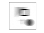
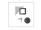
Figure 1: Reconstruction of a blurred test image with $N^{2}=128^{2}$ pixels containing $5\%$ of noise using Algorithm modBSSN with regularization parameter $w=0.9^{33}\approx 0.0309$, $\gamma=10^{5}$ and blurring parameter $L=0.1$. From left to right: original image, blurred noisy image, reconstruction.

We consider an artificially created sparse image with about $15\%$ nonzero entries, the sparseness depends on the number $N^{2}$ of pixels, see Figure 1. Here, the original image of the size $128\times 128$ pixels, the blurred image containing $5\%$ of noise and the reconstruction are presented. The blurring parameter is chosen as $L=0.1$, the regularization parameter is chosen as $w=0.9^{33}\approx 0.0309$ and the parameter $\gamma$ in Algorithm modBSSN is set equal to $10^{5}$.

Table 1: Performance of Algorithm $\mathtt{modBSSN}$ depending on the choice of $\gamma$. The reconstructions are computed for the image from Figure 1 with $128^{2}=16384$ pixels containing $5\%$ of noise, regularization parameter $w=0.9^{33}\approx 0.0309$ and blurring parameter $L=0.1$.

$\gamma$	number of steps	$\#\{j:t_{j}=1\}$
$\texttt{10}^{\texttt{1}}$	113	3
$\texttt{10}^{\texttt{2}}$	23	5
$\texttt{10}^{\texttt{3}}$	12	9
$\texttt{10}^{\texttt{4}}$	12	10
$\texttt{10}^{\texttt{5}}$	11	8
$\texttt{10}^{\texttt{6}}$	11	8
$\texttt{10}^{\texttt{7}}$	13	7

Table 1 demonstrates the performance of Algorithm modBSSN for the image from Figure 1 depending on the choice of $\gamma>0$. The parameter $\gamma$ should not be chosen too small, because the number of Newton steps increases and the amount of steps with stepsize $t_{k}=1$ decreases for smaller $\gamma$. For $\gamma=10^{4}$, the stepsizes are chosen equal to $1$ in $10$ out of $12$ steps.

Table 2: History of the residual norms, the Tikhonov functional values, the stepsizes, the system sizes of the linear complementarity problems (LCP) and of the systems of linear equations (SLE) and the number of linear systems for the image from Figure 1 with $128^{2}=16384$ pixels containing $5\%$ of noise, reconstructed with Algorithm modBSSN with regularization parameter $w=0.9^{33}\approx 0.0309$, the parameter $\gamma=10^{5}$ and $L=0.1$.

$j$	$\|\mathbf{F}(\mathbf{u}^{(j)})\|_{2}$	$J(\mathbf{u}^{(j)})$	$t_{j}$	size of LCP	size of SLE	$\#$ SLE
0	2.3200e+06	357.1522	-	-	-	-
1	8.8461e+02	105.8198	1	0	6043	1
2	7.9131e+02	76.3797	1	616	3944	12441
3	5.7716e+02	66.8937	0.5	441	3161	13224
4	4.2644e+02	59.0065	0.5	321	2769	13616
5	2.3887e+02	51.8326	1	220	2574	13811
6	2.0991e+02	49.7913	0.5	90	2452	13933
7	1.8523e+02	47.4883	1	67	2376	14009
8	4.8111e+01	46.7994	1	22	2357	14028
9	4.1728e-01	46.4408	1	13	2330	14055
10	2.4710e-01	46.4212	1	0	2326	1
11	4.5635e-10	46.4061	1	0	2325	1

The strict decrease of the residual norm in Algorithm modBSSN for the image from Figure 1 with $128^{2}=16384$ pixels is demonstrated in Table 2. Here, the Tikhonov functional values

$$J(\mathbf{u}^{(j)}):=\frac{1}{2}\|\mathbf{K}\mathbf{u}^{(j)}-\mathbf{f}^{\delta}\|_{2}^{2}+w\|\mathbf{u}^{(j)}\|_{1},\quad j=0,1,\ldots$$

are strictly decreasing as well, but this is not guaranteed in general. The stepsizes are eventually chosen equal to $1$ ensuring the locally quadratic convergence of Algorithm modBSSN. The sizes of the linear complementarity problem (LCP), see (28), and of the systems of linear equations (SLE), solved in each step of Algorithm modBSSN to compute the matrix $\mathbf{N}$ from (3), the vector $\mathbf{z}$ from (30) and the Newton direction (39), are usually decreasing in the course of the iteration. Regarding the number $128^{2}=16384$ of pixels, these systems are small. This is due to the structure of Algorithm modBSSN. Because of the starting vector $\mathbf{u}^{(0)}=\mathbf{0}$, the set $\overline{\mathcal{I}^{\pm}}(\mathbf{u}^{(0)})$ is usually empty so that there is usually no LCP to solve in the first step. For other starting vectors $\mathbf{u}^{(0)}$, the size of the LCP in the first step may be larger. If a linear complementarity problem is set up in step $j$, additionally $|\overline{\mathcal{I}}(\mathbf{u}^{(j)})|$ linear systems with the same matrix have to be solved, cf. Section 2.3.

In Table 3, five algorithms for the deblurring of the noisy image from Figure 1 are compared: Algorithm modBSSN and Algorithm hybridBSSN with the choice $\gamma=10^{5}$, the globalized semismooth Newton method (BSSN) from [28] with the choice $\gamma=10^{5}$, sparse reconstruction by separable approximation (SpaRSA) from [54] and Barzilai-Borwein gradient projection for sparse reconstruction (GPSR$\_$BB) from [20]. Note that runtime is implementation-dependent. Note also that BSSN differs from modBSSN only in the choice of the index sets (11)–(15) resp. the modified index sets (23)–(27). By the modification of the index sets, the theoretical drawback that BSSN may fail to converge was eliminated. Therefore, one has to solve mixed linear complementarity problems instead of solving only systems of linear equations. In practice, applying BSSN, complementarity problems usually do not appear. The stopping criterion of Algorithm modBSSN, Algorithm hybridBSSN and Algorithm BSSN is a residual norm $\|\mathbf{F}(\mathbf{u}^{(j)})\|_{2}<10^{-7}$. The other three algorithms are terminated if the Tikhonov functional value falls below the threshold $J^{*}+10^{-7}$, where $J^{*}$ denotes the Tikhonov functional value of hybridBSSN at convergence. The average runtime (clock time) of five runs with starting vector $\mathbf{u}^{(0)}=\mathbf{0}$, the Tikhonov functional value $J_{end}$ at termination, the difference of $J_{end}$ to $J^{*}$, the number of iterations and the number of zeros of the computed solution are listed for the different algorithms. All algorithms produce sparse solutions with $14059$ resp. $14057$ zero components, i.e. about $14.2\%$ nonzero entries. The semismooth Newton methods need only few iterations compared to the other methods. The fastest algorithms are BSSN and hybridBSSN followed by SpaRSA, modBSSN and GPSR$\_$BB. The runtime of Algorithm modBSSN may be improved by using another solver for the linear complementarity problems. In Table 3 and in the following runtime measurements, the computation of the regularization parameter by the discrepancy principle is not included in the listed runtimes. The runtimes are measured with the MATLAB command tic toc.

Table 3: Comparison of different algorithms for the deblurring of the image from Figure 1 with $N=128^{2}$ pixels, $5\%$ of noise, blurring parameter $L=0.1$ and regularization parameter $w=0.9^{33}\approx 0.0309$. The starting vector $\mathbf{u}^{(0)}=\mathbf{0}$ is chosen for all algorithms.

algorithm	average runtime(s)	$J_{end}$	$J_{end}-J^{*}$	$\#$ iterations	$\#$ zeros
modBSSN	8.54	46.4061	1.4211e-14	11	14059
BSSN	0.32	46.4061	0	13	14059
hybridBSSN	0.32	46.4061	0	13	14059
SpaRSA	1.96	46.4061	9.6221e-08	1057	14057
GPSR$\_$BB	15.21	46.4061	9.9948e-08	6352	14059

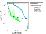
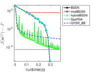
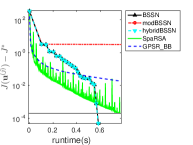
Figure 2: Runtime history of the difference of the Tikhonov functional values and $J^{*}$ for different noise levels $\delta$. From left to right: $\delta=10\%$, $5\%$, $1\%$. The gray line marks the target $2\delta^{2}$ in each case.

The runtime history of the difference $J(\mathbf{u}^{(j)})-J^{*}$ of the Tikhonov functional values $J(\mathbf{u}^{(j)})$ of the algorithms considered in Table 3 to the Tikhonov functional value $J^{*}$ of Algorithm hybridBSSN at convergence is shown in Figure 2 for different noise levels $\delta=10\%$, $5\%$, $1\%$. The parameter $\gamma$ in the algorithms BSSN, modBSSN and hybridBSSN is chosen equal to $10^{5}$ and we set $L=0.1$ and $N^{2}=128^{2}$. Depending on the noise level, it may be adequate to solve the minimization problem only up to an expected accuracy. $\ell_{1}$-Tikhonov regularization with a posteriori parameter choice by the discrepancy principle has a linear convergence rate, see [25], i.e. $\|\mathbf{u}^{\dagger}-\mathbf{u}^{*}_{w,\delta}\|\leq c\delta\|\mathbf{f}\|$, where $c>0$ is a constant, $\mathbf{u}^{\dagger}$ denotes the true solution to $\mathbf{K}\mathbf{u}=\mathbf{f}$ with unperturbed right-hand side $\mathbf{f}$ and $\mathbf{u}^{*}_{w.\delta}$ denotes the solution to (6) with perturbed data $\mathbf{f}^{\delta}$, regularization parameter $w$ and noiselevel $\delta$. Therefore, we decided to minimize the Tikhonov functional up to an accuracy of $2\delta^{2}$. For high noise levels and $N^{2}=128^{2}$, Algorithm SpaRSA outperforms BSSN and hybridBSSN because it reaches the target first. If the minimization problem is solved more accurately in case of smaller noise levels or if the number $N^{2}$ of pixels increases, BSSN and hybridBSSN are advantageous in terms of runtime in this example, cf. Figure 3.

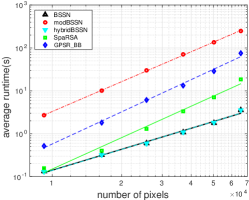
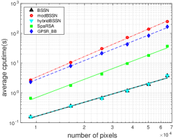
Figure 3: Average runtime and average cputime of $5$ runs depending on the number $N^{2}=(32k)^{2}$, $k=3,\ldots,8$ of pixels for images containing $5\%$ of noise.

Figure 3 presents a clock time and a cputime comparison of the considered algorithms for increasing image sizes $N^{2}=(32k)^{2}$, $k=3,\ldots,8$. The cputime is measured with the MATLAB subroutine cputime. Once again, the blurring parameter is $L=0.1$ and the images contain $5\%$ of noise. The starting vector is $\mathbf{u}^{(0)}=\mathbf{0}$ for all methods, the stopping criterion $J(\mathbf{u}^{(j)})\leq J^{*}+2\delta^{2}$ for GPSR$\_$BB and SpaRSA is chosen as in Figure 2 and we choose $\gamma=10^{4}$ and the stopping criterion $\|\mathbf{F}(\mathbf{u}^{(j)})\|_{2}<10^{-7}$ for BSSN, hybridBSSN and modBSSN. Again, the average runtimes resp. cputimes of $5$ runs are shown. Algorithms BSSN and hybridBSSN outperform the other algorithms regarding cputime in this example, followed by SpaRSA, GPSR$\_$BB and modBSSN. However, SpaRSA and GPSR$\_$BB are better parallelizable than the B-semismooth Newton methods.

4.2 Robust regression

Given data $\mathbf{a}_{1},\ldots,\mathbf{a}_{m}\in\mathbb{R}^{n}$ and $\mathbf{y}\in\mathbb{R}^{m}$, $m\geq n$, our aim is to fit a linear model $\mathbf{A}\mathbf{u}=\mathbf{y}$ with $\mathbf{u}\in\mathbb{R}^{n}$ and $\mathbf{A}=(\mathbf{a}_{1}\cdots\mathbf{a}_{m})^{\top}\in\mathbb{R}^{m\times n}$ to the given data. Errors in data collection may cause outliers, and robust M-estimators give less influence to outliers than the ordinary least squares approach [23]. Here, we choose the well-known $L_{1}$-$L_{2}$ estimator, see e.g. [10]. For a parameter $\rho>0$, the measure function $\varphi_{\rho}\colon\mathbb{R}\to\mathbb{R}^{+}_{0}$, $\varphi_{\rho}(x):=2(\sqrt{\rho+x^{2}/2}-\sqrt{\rho})$ fulfills the conditions $\varphi_{\rho}(x)=\varphi_{\rho}(-x)$ and $\varphi_{\rho}$ is strictly convex [2, 10]. We choose $\rho=1$ and the discrepancy term $g\colon\mathbb{R}^{n}\to\mathbb{R}$,

$$g(\mathbf{u}):=\frac{1}{m}\sum\limits_{k=1}^{m}\varphi_{1}(\mathbf{a}_{k}^{\top}\mathbf{u}-y_{k})=\frac{2}{m}\sum\limits_{k=1}^{m}\Big{(}\sqrt{1+(\mathbf{a}_{k}^{\top}\mathbf{u}-y_{k})^{2}/2}-1\Big{)}.$$

To additionally obtain a sparse regression model, we add an $\ell_{1}$-penalty term

$$\min\limits_{\mathbf{u}\in\mathbb{R}^{n}}g(\mathbf{u})+w\|\mathbf{u}\|_{1},$$ (56)

cf. (10), where the parameter $w>0$ acts as regularization parameter, see e.g. [1, 37]. In the following, we assume that $\mathbf{A}=(\mathbf{a}_{1}\cdots\mathbf{a}_{m})^{\top}\in\mathbb{R}^{m\times n}$ is injective. Then, the Hessian $\nabla^{2}g(\mathbf{u})$ is positive definite for all $\mathbf{u}\in\mathbb{R}^{n}$. However, it is not ensured that the level sets of $\Theta$ stay bounded. The data $\mathbf{a}_{1},\ldots,\mathbf{a}_{m}\in\mathbb{R}^{n}$ are chosen normally distributed with standard deviation $1$ and mean $0$. We compute $\mathbf{y}^{\delta}=\mathbf{A}\mathbf{u}+\mathbf{e}$, where $\mathbf{e}\sim\mathcal{N}(0,1)$ and for a portion of the entries of $\mathbf{y}^{\delta}$ we choose $\mathbf{e}\sim\mathcal{N}(0,50)$, i.e. we construct outliers.

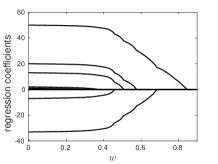
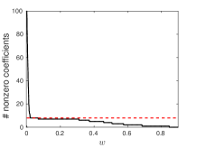
Figure 4: Sparsity of the regression model depending on the choice of the regularization parameter $w$. Left: path of the computed regression coefficients. Right: number of nonzero regression coefficients (red dashed line: number of nonzero coefficients of the true regression model).

If the underlying model is unknown, there are several possibilities to select the regularization parameter $w$. For example, cross-validation may be used as proposed in [1, 51]. Here, we assume that the true model is known. Similar to the parameter choice strategy proposed in [36], we choose the regularization parameter $w$ so that $\#\{k:(\mathbf{u}_{w})_{k}\neq 0\}$ is equal to the number of nonzero elements of the true solution and $\mathbf{u}_{w}$ has minimal standard error

$$\sigma=\sqrt{\frac{1}{m-n-1}\sum_{k=1}^{m}(\mathbf{a}_{k}^{\top}\mathbf{u}_{w}-y_{k})^{2}},$$ (57)

respectively maximal $R^{2}$-value

$$R^{2}=1-\frac{\frac{1}{m-n-1}\sum\limits_{k=1}^{m}(\mathbf{a}_{k}^{\top}\mathbf{u}_{w}-y_{k})^{2}}{\frac{1}{m-1}\sum\limits_{k=1}^{m}(\overline{y}-y_{k})^{2}},$$ (58)

where $\mathbf{u}_{w}$ denotes the vector of computed regression coefficients for the regularization parameter $w$. Therefore, we minimize (56) for $w=\nu/10000$, $\nu=1,\ldots,9000$ and choose the starting vector $\mathbf{u}^{(0)}$ for $\nu>1$ as the solution to (56) of the last computation with $w=(\nu-1)/10000$. The true model is of the size $m=10000$, $n=100$ and has $8$ nonzero coefficients with weights $-33$, $-7$, $-0.1$, $1$, $2$, $13$, $20$ and $50$. The noisy vector $\mathbf{y}^{\delta}$ contains $10\%$ outliers. Figure 4 demonstrates the influence of the regularization parameter $w>0$ on the sparsity of the regression model. For the computations, we set $\gamma=10$ and the tolerance equal to $10^{-7}$ in Algorithm modBSSN. For very small $w$, all coefficients are chosen nonzero. If $w$ is chosen larger than $0.8474$, all coefficients are chosen equal to zero.

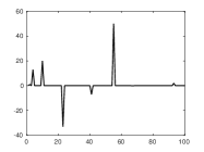
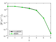
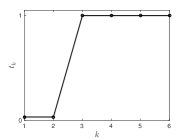
Figure 5: Illustration of the performance of Algorithm $\mathtt{modBSSN}$ and Algorithm $\mathtt{BSSN}$ with $w=0.0201$ and $\gamma=10$ for the robust regression example. From left to right: true regression coefficients, residual norms, chosen stepsizes (identical for both algorithms).

Figure 5 shows the convergence properties of Algorithm modBSSN and the B-semismooth Newton method (BSSN) from Section 2.2 for the example from Figure 4. We choose $w=0.0201$ and $\gamma=10$. Both algorithms converge within $6$ steps and the chosen stepsizes of the two algorithms coincide in this example. The stepsizes are four times chosen equal to $1$. For other values of $\gamma$, more Newton steps need to be computed.

5 Conclusion

In the present paper, we are concerned with the efficient minimization of functionals of the type (1). In [28], a globalized B-semismooth Newton method was presented for quadratic discrepancy terms. Here, we generalized the method from [28] to nonquadratic discrepancy terms. Additionally, by modifying index subsets, a modified algorithm was shown to be globally convergent without any additional requirements on the a priori unknown accumulation point of the sequence of iterates. Thus, we have overcome a theoretical drawback of [28] concerning global convergence. Another advantage of the presented modified method is its local convergence speed. If an additional assumption is fulfilled, we have shown that the stepsizes are chosen eventually equal to $1$ and locally quadratic convergence is achieved.

By design, the proposed modified B-semismooth Newton method requires the solution of one linear complementarity problem per iteration, instead of one linear system as in other generalized Newton schemes. However, we have demonstrated that these systems stay small relative to the number of unknowns and therefore do not spoil the overall complexity. A hybrid version combines the efficiency of the B-semismooth Newton method and the convergence properties of the modified method.

In further research, one may focus on the development of globally convergent inexact Newton methods as proposed in [15] for the smooth case enabling the design of matrix-free variants. Moreover, the globalization of quasi-Newton methods like [40] could be considered.

References

- [1] A. Alfons, C. Croux, and S. Gelper. Sparse least trimmed squares regression for analyzing high-dimensional large data sets. Ann. Appl. Stat., 7(1):226–248, 2013.
- [2] Ö. G. Alma. Comparison of robust regression methods in linear regression. Int. J. Contemp. Math. Sciences, 6(9):409–421, 2011.
- [3] S. W. Anzengruber and R. Ramlau. Morozov’s discrepancy principle for Tikhonov-type functionals with nonlinear operators. Inverse Problems, 26(2):025001, 2010.
- [4] A. Beck and M. Teboulle. A fast iterative shrinkage-thresholding algorithm for linear inverse problems. SIAM J. Imaging Sci., 2(1):183–202, 2009.
- [5] T. Bonesky. Morozov’s discrepancy principle and Tikhonov-type functionals. Inverse Problems, 25(1):015015, 2009.
- [6] T. Bonesky, K. Bredies, D. A. Lorenz, and P. Maass. A generalized conditional gradient method for nonlinear operator equations with sparsity constraints. Inverse Problems, 23(5):2041–2058, 2007.
- [7] T. Bonesky, S. Dahlke, P. Maass, and T. Raasch. Adaptive wavelet methods and sparsity reconstruction for inverse heat conduction problems. Adv. Comput. Math., 33(4):385–411, 2010.
- [8] K. Bredies, D. A. Lorenz, and P. Maass. A generalized conditional gradient method and its connection to an iterative shrinkage method. Comput. Optim. Appl., 42(2):173–193, 2009.
- [9] X. Chen, Z. Nashed, and L. Qi. Smoothing methods and semismooth methods for nondifferentiable operator equations. SIAM J. Numer. Anal., 38(4):1200–1216, 2000.
- [10] K. L. Clarkson and D. P. Woodruff. Sketching for M-estimators: a unified approach to robust regression. In P. Indyk, editor, Proceedings of the Twenty-Sixth Annual ACM-SIAM Symposium on Discrete Algorithms, pages 921–939. SIAM, 2015.
- [11] P. L. Combettes and V. R. Wajs. Signal recovery by proximal forward-backward splitting. Multiscale Model. Simul., 4(4):1168–1200, 2005.
- [12] R. W. Cottle, J.-S. Pang, and R. E. Stone. The linear complementarity problem. Philadelphia, SIAM, 2009.
- [13] I. Daubechies, M. Defrise, and C. De Mol. An iterative thresholding algorithm for linear inverse problems with a sparsity constraint. Comm. Pure Appl. Math., 57(11):1413–1457, 2004.
- [14] S. P. Dirkse and M. C. Ferris. The path solver: a nonmonotone stabilization scheme for mixed complementarity problems. Optim. Methods Softw., 5(2):123–156, 1995.
- [15] S. C. Eisenstat and H. F. Walker. Globally convergent inexact Newton methods. SIAM J. Optim., 4(2):393–422, 1994.
- [16] H. W. Engl, M. Hanke, and A. Neubauer. Regularization of inverse problems, volume 375 of Mathematics and its Applications. Dordrecht, Kluwer Academic Publishers, 1996.
- [17] F. Facchinei and J.-S. Pang. Finite-dimensional variational inequalities and complementarity problems, volume 1. New York, Springer, 2003.
- [18] F. Facchinei and J.-S. Pang. Finite-dimensional variational inequalities and complementarity problems, volume 2. New York, Springer, 2003.
- [19] M. C. Ferris and T. S. Munson. Interfaces to PATH 3.0: design, implementation and usage. Comput. Optim. Appl., 12(1):207–227, 1999.
- [20] M. A. T. Figueiredo, R. D. Nowak, and S. J. Wright. Gradient projection for sparse reconstruction: application to compressed sensing and other inverse problems. IEEE J. Sel. Topics Signal Process., 1(4):586 – 597, 2007.
- [21] A. Fischer. A Newton-type method for positive-semidefinite linear complementarity problems. J. Optim. Theory Appl., 86(3):585–608, 1995.
- [22] A. Fischer and C. Kanzow. On finite termination of an iterative method for linear complementarity problems. Math. Program., 74(3):279–292, 1996.
- [23] J.-J. Fuchs. An inverse problem approach to robust regression. In Proceedings of the IEEE International Conference on Acoustics, Speech, and Signal Processing, Phoenix, volume 4, pages 1809–1812. IEEE, 1999.
- [24] M. Gehre, T. Kluth, A. Lipponen, B. Jin, A. Seppänen, J. P. Kaipio, and P. Maass. Sparsity reconstruction in electrical impedance tomography: An experimental evaluation. J. Comput. Appl. Math., 236(8):2126–2136, 2012.
- [25] M. Grasmair, O. Scherzer, and M. Haltmeier. Necessary and sufficient conditions for linear convergence of -regularization. Comm. Pure Appl. Math., 64(2):161–182, 2011.
- [26] R. Griesse and D. A. Lorenz. A semismooth Newton method for Tikhonov functionals with sparsity constraints. Inverse Problems, 24(3):035007, 2008.
- [27] S.-P. Han, J.-S. Pang, and N. Rangaraj. Globally convergent Newton methods for nonsmooth equations. Math. Oper. Res., 17(3):586–607, 1992.
- [28] E. Hans and T. Raasch. Global convergence of damped semismooth Newton methods for Tikhonov regularization. Inverse Problems, 31(2):025005, 2015.
- [29] P. C. Hansen. Deconvolution and regularization with Toeplitz matrices. Numer. Algorithms, 29(4):323–378, 2002.
- [30] P. T. Harker and J.-S. Pang. A damped-Newton method for the linear complementarity problem. In E. L. Allgower and K. Georg, editors, Computational solution of nonlinear systems of equations, volume 26 of Lectures in Appl. Math., pages 265–284. Providence, Amer. Math. Soc., 1990.
- [31] D. N. Hào and T. N. T. Quyen. Convergence rates for Tikhonov regularization of coefficient identification problems in Laplace-type equations. Inverse Problems, 26(12):125014, 2010.
- [32] K. Ito and K. Kunisch. On a semi-smooth Newton method and its globalization. Math. Program., Ser. A, 118(2):347–370, 2009.
- [33] B. Jin, T. Khan, and P. Maass. A reconstruction algorithm for electrical impedance tomography based on sparsity regularization. Int. J. Numer. Methods Eng., 89(3):337–353, 2012.
- [34] B. Jin and P. Maass. Sparsity regularization for parameter identification problems. Inverse Problems, 28(12):123001, 2012.
- [35] I. Knowles. Parameter identification for elliptic problems. J. Comput. Appl. Math., 131:175 – 194, 2001.
- [36] V. Kolehmainen, M. Lassas, K. Niinimäki, and S. Siltanen. Sparsity-promoting Bayesian inversion. Inverse Problems, 28(2):025005, 2012.
- [37] Y.-H. Li, J. Scarlett, P. Ravikumar, and V. Cevher. Sparsistency of -regularized M-estimators. In G. Lebanon and S. V. N. Vishwanathan, editors, Proceedings of the Eighteenth International Conference on Artificial Intelligence and Statistics, San Diego, volume 38, pages 644–652. JMLR Workshop and Conference Proceedings, 2015.
- [38] D. A. Lorenz, P. Maass, and P. Q. Muoi. Gradient descent for Tikhonov functionals with sparsity constraints: theory and numerical comparison of step size rules. Electron. Trans. Numer. Anal., 39:437–463, 2012.
- [39] A. Milzarek and M. Ulbrich. A semismooth Newton method with multidimensional filter globalization for -optimization. SIAM J. Optim., 24(1):298–333, 2014.
- [40] P. Q. Muoi, D. N. Hào, P. Maass, and M. Pidcock. Semismooth Newton and quasi-Newton methods in weighted -regularization. J. Inverse Ill-Posed Probl., 21(5):665–693, 2013.
- [41] Y. Nesterov. Gradient methods for minimizing composite functions. Math. Program., Ser. B, 140(1):125–161, 2013.
- [42] M. R. Osborne, B. Presnell, and B. A. Turlach. A new approach to variable selection in least squares problems. IMA J. Numer. Anal., 20(3):389–404, 2000.
- [43] J.-S. Pang. Newton’s method for B-differentiable equations. Math. Oper. Res., 15(2):pp. 311–341, 1990.
- [44] J.-S. Pang. A B-differentiable equation-based, globally and locally quadratically convergent algorithm for nonlinear programs, complementarity and variational inequality problems. Math. Program., 51(1):101–131, 1991.
- [45] L. Qi. Convergence analysis of some algorithms for solving nonsmooth equations. Math. Oper. Res., 18(1):227–244, 1993.
- [46] L. Qi and J. Sun. A nonsmooth version of Newton’s method. Math. Program., 58(3):353–367, 1993.
- [47] D. Ralph. Global convergence of damped Newton’s method for nonsmooth equations via the path search. Math. Oper. Res., 19(2):352–389, 1994.
- [48] R. Ramlau and G. Teschke. A Tikhonov-based projection iteration for nonlinear ill-posed problems with sparsity constraints. Numer. Math., 104(2):177–203, 2006.
- [49] T. Schuster, B. Kaltenbacher, B. Hofmann, and K. S. Kazimierski. Regularization methods in Banach spaces, volume 10 of Radon Series on Computational and Applied Mathematics. Berlin, de Gruyter, 2012.
- [50] A. Shapiro. On concepts of directional differentiability. J. Optim. Theory Appl., 66(3):477–487, 1990.
- [51] R. Tibshirani. Regression shrinkage and selection via the Lasso. J. R. Statist. Soc. Ser. B Met., 58(1):267–288, 1996.
- [52] M. Ulbrich. Nonsmooth Newton-like methods for variational inequalities and constrained optimization problems in function spaces. Habilitation thesis, Technical University Munich, Munich, 2002.
- [53] J. Williams, Y. Lu, S. Niebe, M. Andersen, K. Erleben, and J. C. Trinkle. RPI-MATLAB-Simulator: A Tool for Efficient Research and Practical Teaching in Multibody Dynamics. In J. Bender, J. Dequidt, C. Duriez, and G. Zachmann, editors, Workshop on Virtual Reality Interaction and Physical Simulation, pages 71–80. The Eurographics Association, 2013.
- [54] S. J. Wright, R. D. Nowak, and M. A. T. Figueiredo. Sparse reconstruction by separable approximation. IEEE Trans. Signal Process., 57(7):2479–2493, 2009.
- [55] J. Yang and Y. Zhang. Alternating direction algorithms for -problems in compressive sensing. SIAM J. Sci. Comput., 33(1):250–278, 2011.