Regularized integral formulation of mixed Dirichlet-Neumann problems
Abstract
This paper presents a theoretical discussion as well as novel solution algorithms for problems of scattering on smooth two-dimensional domains under Zaremba boundary conditions—for which Dirichlet and Neumann conditions are specified on various portions of the domain boundary. The theoretical basis of the proposed numerical methods, which is provided for the first time in the present contribution, concerns detailed information about the singularity structure of solutions of the Helmholtz operator under boundary conditions of Zaremba type. The new numerical method is based on use of Green functions and integral equations, and it relies on the Fourier Continuation method for regularization of all smooth-domain Zaremba singularities as well as newly derived quadrature rules which give rise to high-order convergence even around Zaremba singular points. As demonstrated in this paper, the resulting algorithms enjoy high-order convergence, and they can be used to efficiently solve challenging Helmholtz boundary value problems and Laplace eigenvalue problems with high-order accuracy.
1 Introduction
This paper concerns problems of scattering on smooth two-dimensional domains under Zaremba boundary conditions, and, in particular, it presents a theoretical discussion as well as novel solution algorithms for this problem. The theoretical basis of the proposed numerical methods concerns detailed information, put forth in Section 4, about the singularity structure of the solutions of the Helmholtz operator under boundary conditions of Zaremba type. The new numerical method, which is based on use of Green functions and integral equations, incorporates use of the Fourier Continuation method for regularization of all smooth-domain Zaremba singularities as well as newly derived quadrature rules which give rise to high-order convergence even around Zaremba singular points. As demonstrated in this paper, the resulting algorithms enjoy high-order convergence, and they can used to efficiently solve challenging Helmholtz boundary value problems and Laplace eigenvalue problems with high-order accuracy.
We thus consider the classical Zaremba boundary value problem
| (1.1) |
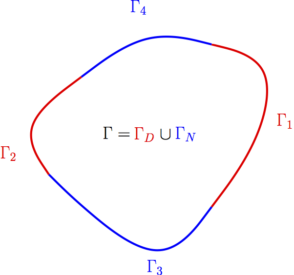
for the Helmholtz equation, where is a 2-dimensional domain with boundary consisting of two disjoint portions and upon which Dirichlet and Neumann values are prescribed, respectively; see Figure 1.
Significant challenges arise in connection with Zaremba boundary value problems in view of the singular character of its solutions: as first established by Fichera [14], Zaremba solutions are generally non-smooth even for infinitely differentiable boundary data and , and smoothness of solutions can only be ensured provided and obey certain relations which generically are not satisfied. Wigley [29, 30] provides a detailed description of the singularity structure around Zaremba points—which includes singularities of both square-root and logarithmic type. In Section 4 of the present paper it is shown, however, that a tighter result holds in the case the domain boundary is itself smooth.
Problems with mixed Dirichlet-Neumann boundary conditions were first considered in Zaremba’s 1910 contribution [32], which established existence and uniqueness of solution in the particular case of the Laplace equation (). Boundary conditions of Zaremba type arise in a number of important areas, including elasticity theory (were it appears as a model in the contexts of contact mechanics [28] and crack theory [12]); homogenization theory (as it applies to problems of steady state diffusion through perforated membranes [12]), etc. One of the main motivations for our consideration of this problem concerns computational electromagnetism: the Zaremba problem serves as a valuable stepping stone to the closely related but more complex problem of electromagnetic propagation and scattering at and around structures such as printed circuit-boards. (As in the Zaremba problem, where the boundary conditions change type at the Dirichlet-Neumann boundary, the boundary conditions for the Maxwell equations at and around circuit-boards change type—not from Dirichlet to Neumann but from dielectric transmission conditions to perfect-conductor conditions—at the edges of the perfectly conducting circuit elements.)
After the initial contribution by Zaremba, early works concerning the Zaremba boundary value problem include results by Signorini [25] (1916: solution of the Zaremba problem in the upper half plane using complex variable methods); Giraud [17] (1934: existence of solution of Zaremba problems for general elliptic operators); Fichera [13, 14] (1949, 1952: regularity studies at Zaremba points, Zaremba-type problem for the elasticity equations in two spatial dimensions); Magenes [22] (1955: proof of existence and uniqueness, single layer potential representation); Lorenzi [21] (1975: Sobolev regularity around a corner which is also a Dirichlet-Neumann junction); and Wigley [29, 30] (1964, 1970: explicit asymptotic expansions around Dirichlet-Neumann junctions), amongst others. More recent contributions in this area include reference [28], which provides a valuable review in addition to a study of Zaremba singularities and theoretical results concerning Galerkin-based computational approaches; reference [7], which considers the Zaremba problem for the biharmonic equation; references [10, 11], which study Zaremba boundary value problems for Helmholtz and Laplace-Beltrami equations; reference [8], which discusses the solvability of the Zaremba problem from the point of view of pseudo-differential calculus and Sobolev regularity theory; reference [18] which introduces a certain inverse preconditioning technique to reduce the number of linear algebra iterations for the iterative numerical solution of this problem and which gives rise to high-order convergence; and finally, reference [4], which successfully applies the method of difference potentials to the variable-coefficient Zaremba problem, with convergence order approximately equal to one.
The rest of this paper is organized as follows: after some necessary preliminaries presented in Section 2, Section 3 lays down the integral equation system we use, and it studies the equivalence between the integral equation system and the original Zaremba problem (1.1). Detailed asymptotics for the Zaremba singularities at Dirichlet-Neumann junction are presented in Section 4. Building upon these results, further, and exploiting an interesting connection of this problem with the Fourier-Continuation method [6, 3], Fourier expansions for the integral densities are obtained in Section 5 which regularize all Zaremba singularities. Section 6 then introduces a numerical algorithm that incorporates the aforementioned Fourier Continuation series on the basis of certain closed form integral expressions, and which thus produces numerical solutions with high-order accuracy. A variety of results in Section 7 demonstrates the quality of the solutions and Zaremba eigenfunctions produced by the proposed numerical approach, and Section 8, finally, presents a few concluding remarks.
2 Preliminaries
We consider interior and exterior boundary value problems of the form given in equation (1.1) for (with a Sommerfeld radiation condition in case of exterior problems), where denotes either a bounded, open and simply-connected domain with a smooth boundary (which we will generically call an “interior” domain) or the complement of the closure of such a domain (an “exterior” domain), where the Dirichlet and Neumann boundary portions and () are disjoint relatively-open subsets of of positive measure relative to . Here, calling the ball of radius centered at the origin, we have denoted by
| (2.1) |
the local Sobolev space of order one; of course for bounded sets . The Dirichlet and Neumann data and in (1.1), in turn, are elements of certain Sobolev spaces (cf. Remark 2.1 item ii) which we define in what follows. To do this we follow [23] and we first define, for a given relatively open subset , the space
The spaces associated with the Dirichlet and Neumann data and are then defined by
and, using the prime notation to denote the dual space of a given Hilbert space ,
respectively.
Remark 2.1.
Throughout this paper …
-
(i)
…the term “smooth” is equated to “infinitely differentiable ” and, as indicated above, it is assumed that the boundary of the domain is smooth.
- (ii)
The boundary can be expressed in the form
| (2.2) |
where and denote the numbers of smooth connected Dirichlet and Neumann boundary portions, and where for (resp. for ), denotes a Dirichlet (resp. Neumann) portion of the boundary curve (see e.g. Figure 1). Clearly, letting
we have that
are the subsets of upon which Dirichlet and Neumann boundary conditions are enforced, respectively. Note that consecutive values of the index do not necessarily correspond to consecutive boundary segments. Throughout this paper it is assumed, however, that no Dirichlet-Dirichlet or Neumann-Neumann junctions occur, and, thus, that every endpoint of a segment coincides with a Dirichlet-Neumann junction. Clearly this is not a restriction: consecutive Dirichlet (resp. Neumann) segments can be combined to produce a partition which verifies the assumptions above.
Remark 2.2.
In case is an exterior domain, problem (1.1) admits unique solutions in . On the other hand, if is an interior domain, this problem is not well posed for a discrete set of real values , —the squares of which are the Zaremba eigenvalues, that is to say, the eigenvalues of the Laplace operator under the corresponding homogeneous mixed Dirichlet-Neumann (Zaremba) boundary conditions (see [23, Th. 4.10], [1]).
3 Boundary integral equation formulation
In what follows we seek solutions of problem (1.1) on the basis of the single-layer potential representation
| (3.1) |
where is the Helmholtz Green function in two-dimensional space. Taking into account well known expressions [9, p. 40] for the jump of the single layer potential and its normal derivative across , the boundary conditions for the exterior (resp. interior) boundary value problem (1.1) give rise to the integral equations
| (3.2) |
with (resp. ).
Important properties of both the interior and exterior integral equation problems (3.2) relate to existence of eigenvalues of certain interior problems for the Laplace operator under either Dirichlet or Zaremba boundary conditions. As shown in what follows, for example,
-
1.
In case is an exterior domain the integral equation system (3.2) admits unique solutions if and only if is not a Dirichlet eigenvalue of the Laplace operator in .
- 2.
-
3.
In case is an interior domain, in turn, the integral equation system is uniquely solvable provided is not a Zaremba eigenvalue of the Laplace operator in .
-
4.
The PDE problem (1.1) in such an interior domain does not admit unique solutions, of course, for values of for which is a Zaremba eigenvalue in . In this case the eigenfunctions of the Zaremba Laplace operator can be expressed in terms of the representation formula (3.1) for a certain density which satisfies (3.2) with and .
A detailed treatment concerning points 1, 3 and 4 above is presented in the remainder of this section (Theorems 3.3, 3.4 and Definition 3.1). A corresponding discussion concerning point 2, in turn, is put forth in Appendix A.
Definition 3.1.
Given an interior (resp. exterior) domain and a solution of (1.1) in , a function is said to be a solution “conjugate” to if it satisfies
| (3.3) |
as well as, in case is an exterior domain, Sommerfeld’s condition of radiation at infinity. Throughout this paper the conjugate solution in case is an exterior (resp. interior) domain will be denoted by (resp. ).
Lemma 3.2.
The conjugate solutions mentioned in Definition 3.1 exist and are uniquely determined in each one of the following two cases:
-
1.
is an exterior domain; and
-
2.
is an interior domain and is not a Dirichlet eigenvalue of the Laplace operator in .
Proof.
For both point 1 and point 2 we rely on the fact that the solution of the problem (1.1) is in (see Remark 2.2), and, therefore, by the trace theorem (e.g. [23, Th 3.37]), its boundary values lie in . For point 1 we then invoke [23, Th 9.11] to conclude that a uniquely determined conjugate solution exists, as needed. Point 2 follows similarly using [23, Th 4.10] under the assumption that is not a Dirichlet eigenvalue in the interior domain . ∎
Theorem 3.3.
Let be an exterior domain, and let be such that is not a Dirichlet eigenvalue of the Laplace operator in the interior domain . Then the exterior integral equation system (3.2) (, see also Remark 2.1 item ii) admits a unique solution given by
| (3.4) |
where is the solution of the exterior mixed problem (1.1), and where is the (uniquely determined) corresponding conjugate solution (Definition 3.1 and Lemma 3.2).
Proof.
To obtain (3.4) we first consider the Green representation formula for the functions and ,
| (3.5) |
which, in view of the jump relations for the single and double layer potential operators, in the limit leads to the relations
| (3.6) |
Since for we have , the sum of the two equations in (3.6) yields
| (3.7) |
and, thus, in view of (3.4),
| (3.8) |
Similarly, in the limit the normal derivatives of the integrals in (3.5) give rise to the relations
| (3.9) |
The sum of the equations in (3.9) results in the identity
| (3.10) |
or, equivalently,
| (3.11) |
But for we have , and, thus, equation (3.11) can be made to read
| (3.12) |
Equations (3.8) and (3.12) tell us that the density is a solution of the exterior integral equation system (3.2), as claimed.
In order to establish the solution uniqueness let be a solution of equation (3.2) with and . Since as mentioned above the exterior mixed problem is uniquely solvable, the corresponding single layer potential
| (3.13) |
is equal to zero everywhere in . It then follows from the continuity of the single layer potential that satisfies the Dirichlet problem in the interior domain with zero boundary values. Since by assumption is not a Dirichlet eigenvalue of the Laplacian in it follows that in that region as well. Thus, both the interior and exterior normal derivatives vanish, and therefore so does their difference . The proof is now complete. ∎
Theorem 3.4.
Let be an interior domain. Then we have:
-
1.
If is not a Zaremba eigenvalue (see Remark 2.2), then the interior integral equation system (3.2) (=1, see also Remark 2.1 item ii) admits a unique solution, which is given by
(3.14) Here is the solution of the interior mixed problem (1.1), and is the solution conjugate to (Definition 3.1 and Lemma 3.2).
- 2.
Proof.
We first consider properties that are common to Zaremba solutions and eigenfunctions, and which therefore relate to both points 1 and 2 in the statement of the theorem. For any given solution of the interior mixed problem (1.1) ( can be either the unique solution of the interior mixed problem in the case is not an eigenvalue, or any eigenfunction satisfying (1.1) with and ) the conjugate solution is uniquely defined (Lemma 3.2). Letting
| (3.16) |
using the Green representation formula for and ,
| (3.17) |
and taking into account the jump relations for the double layer potential as well as the fact that for we obtain
| (3.18) |
Similarly, taking normal derivatives of both sides of each equation in (3.17) at a point we obtain the equations
| (3.19) |
whose sum yields
| (3.20) |
We now conclude the proof by applying these concepts to points 1 and 2 in the statement of the theorem.
- 1.
- 2.
The proof is now complete. ∎
4 Singularities of the solutions of equations (1.1) and (3.2)
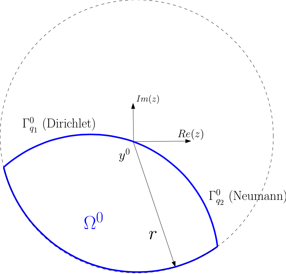
With reference to equation (2.2), let be a point which separates Dirichlet and Neumann regions and ( and ) within . In order to express the singular character around of both the solution of problem (1.1) () and the corresponding integral equation density in equation (3.2) () we consider the neighborhoods
| (4.1) |
of the singular point relative to , and , respectively. Here for a set , denotes the topological closure of in , denotes the circle centered at of radius , and is sufficiently small that only has nonempty intersections with for the Dirichlet index and the Neumann index . Additionally, we use certain functions , and where the Dirichlet (resp. Neumann) function (resp ) is the density as a function of the distance to the point in (resp. ), and where is a complex variable (see Figure 2). The functions , and are given by
| (4.2) |
where, as mentioned above
| (4.3) |
It is known [29, 30] that, under our assumption that the curve is globally smooth, for any given integer the function can be expressed in the form
| (4.4) |
for all in a neighborhood of the origin, where and are -dependent polynomial functions of , , , , , .
Remark 4.1.
In the asymptotic expansion (4.4), and, indeed, in all similar asymptotic expansions in this paper, it is assumed that none of the right hand side polynomials contain terms that, multiplied by the relevant factors, could be included in the error term.
Under our standing assumption of smoothness of the domain boundary the following two theorems provide 1) Finer details on the asymptotics (4.4) as well as 2) A corresponding asymptotic expression around for the solutions and of the integral-equation system (3.2).
Theorem 4.2.
Let be a Dirichlet-Neumann point as described above in this section. Then, given an arbitrary integer , the function can be expressed in the form
| (4.5) |
around , where is an -dependent polynomial function of its arguments; see Remark 4.1.
Theorem 4.3.
Let be a Dirichlet-Neumann point. Then given an arbitrary integer the functions and can be expressed in the forms
| (4.6) |
around , where and are -dependent polynomial functions of their arguments; see Remark 4.1.
Note in particular that Theorem 4.2 shows that, under our assumptions of boundary smoothness, all logarithmic terms in equation (4.4) actually drop out. The proofs of these theorems (which are given in Sections 4.2 and 4.3, respectively) utilize a certain conformal map introduced in Section 4.1 that transforms into a semicircular region.
4.1 Conformal mapping
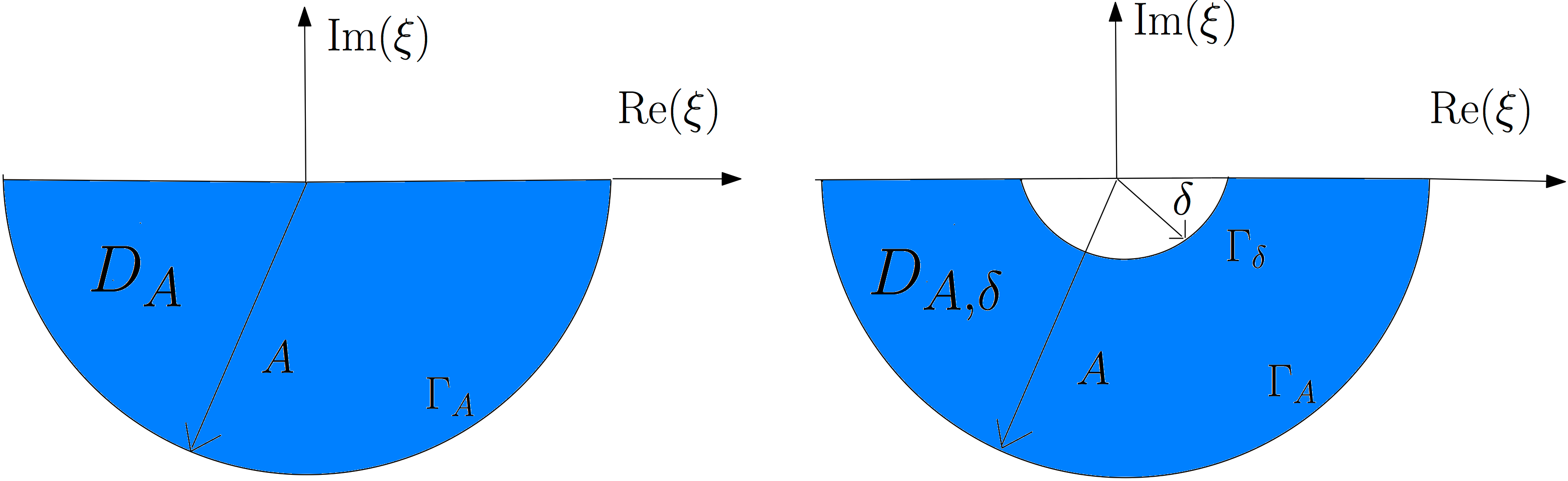
Following [29], in order to establish Theorem 4.2 we identify with the complex plane via the aforementioned relationship , and we utilize a conformal map which maps the semi-circular region ) in the complex -plane (Figure 3) onto the domain (equation (4.1)) in the complex plane. We assume, as we may, that maps the origin to itself and that the intervals and are mapped onto the boundary segments and , respectively.
Letting
| (4.7) |
we note that, in view of the relation satisfied by a complex analytic function (see [15, eq. 5.4.17]), satisfies the second order elliptic equation
| (4.8) | ||||||
| (4.9) | ||||||
| (4.10) | ||||||
| (4.11) |
Here , and . (The function is thus obtained from the restriction of the solution to the set ; see equation (4.1) and Figure 2).
4.2 Proof of theorem 4.2
The proof of this theorem, which, under the present scope of smooth-domain problems establishes a result stronger than [29, Th. 3.2], does incorporate some of the lines of the proof provided in that reference. In what follows we use the Laplace-Zaremba Green function
| (4.12) |
for the lower half plane with homogeneous Dirichlet (resp. Neumann) boundary conditions on the positive (resp.negative) real axis in terms of the complex variables and . The branches of the square roots in (4.12) are given by and where and denote polar coordinates in the complex - and -plane respectively (). Note that, with these conventions the domain in the variables is given by and . The following Lemma establishes certain important properties of the aforementioned Green function.
Lemma 4.4.
The function (equation (4.12)) is indeed a Laplace-Zaremba Green function for the lower half plane with a Dirichlet-Neumann junction at the origin, that is we have and satisfies
| (4.13) |
In addition, for a certain constant we have
| (4.14) |
for all .
Proof.
The function can be re-expressed in the form
| (4.15) |
The first statement in equation (4.13) follows from the relations and , which hold for () since, in view of our selection of branch cuts we have
| (4.16) |
In order to establish the second statement in (4.13) and equation (4.14) we consider the relations
| (4.17) |
which are valid for all complex numbers , and we note that, on the axis we have . Thus, the second statement in (4.13) follows from application of the first equation in (4.17) to each one of the four logarithmic terms that result from expansion of equation (4.15). In order to establish a bound of the form (4.14), finally, we use the second equation in (4.17) to obtain the expression
| (4.18) |
for the absolute value of the derivative of (4.15) with respect to . It is then easy to check that
| (4.19) |
for all . Since the right-hand side of equation (4.19) is uniformly bounded for and since for the integrand in (4.14) vanishes (in view of the second expression in (4.17)), we see that there exists a constant such that equation (4.14) holds for all , as needed, and the proof is thus complete. ∎
The proof of the theorem 4.2 is based on a bootstrapping argument which is initiated by the simple but suboptimal asymptotic relation put forth in the following lemma
Lemma 4.5.
Proof.
To establish this relation we consider the Green formula
| (4.21) |
Since satisfies (4.13) as it befits a Green function for (4.8)–(4.11), denoting by the radius- part of it follows that
| (4.22) |
For the integral over the outer arc in (4.22) we have
| (4.23) |
as it can be checked easily in view of the boundedness of the integrands for near the origin. Taking into account that (see Remark 2.2), on the other hand, it easily follows that , and thus, bounding the absolute value of the first integral in (4.22) by means of the Cauchy-Schwarz inequality, for near we obtain the uniform estimate
| (4.24) |
In order to estimate the second and third integrals in (4.22) we note that the integrals of the absolute values of and are uniformly bounded, as can be checked easily for the former, and as it is established in Lemma 4.4 of the latter. The boundedness of and (which are smooth functions in view of Remark 2.1) thus implies the uniform boundedness of the function near the origin. The relation (4.20) therefore follows for all , and the proof is complete. ∎
Corollary 4.6.
Proof.
See [29, Section 4]. ∎
A key element in the bootstrapping algorithm mentioned at the beginning of this section is a representation formula for the function that is presented in the following Lemma.
Lemma 4.7.
Proof.
Applying the Green formula on the set
| (4.28) |
(right portion of Figure 3) we obtain the expression
| (4.29) |
Further, for fixed we have
| (4.30) |
and therefore, in view of Lemma 4.5 and (4.25),
| (4.31) |
Letting denote the radius- arc within the boundary of (Figure 3), and noting that for we have , in view of (4.31) we obtain
| (4.32) |
Further, exploiting the fact that the Green function (4.12) is a jointly analytic function of and for and around , we obtain
| (4.33) |
where and denote power series with positive radii of convergence.
In order to determine the singular character of around (and therefore that of around ) we study the corresponding asymptotic behavior of each one of the -terms in equation (4.26). An important part of this discussion is the following Lemma, which presents certain regularity properties of the operators , and .
Lemma 4.8.
Let , and , and let or . Then
| (4.35) |
| (4.36) |
| (4.37) |
For general functions and satisfying and as , further, we have
| (4.38) |
| (4.39) |
| (4.40) |
(see Remark 4.1). Here (resp. ), , are power series with positive radii of convergence (resp. polynomials), , are complex constants, and the expansions are -times differentiable as —in the sense of Wigley: the derivatives of the left hand sides in (4.38) through (4.40) are equal to the corresponding derivatives of the first two term of the right hand sides, with error terms given by the “formal” derivatives of the corresponding error terms—e.g. .
We are now ready to provide the main proof of this section.
Proof of Theorem 4.2.
Since the solutions and are related by equation (4.7), using the classical result [27, Th. IV] (which establishes, in particular, that the conformal mapping is smooth up to and including the boundary for any smooth segment of the domain boundary; see also [26]) and expanding in Taylor series around , we see that it suffices to prove that for an arbitrary integer we have the asymptotic relation
| (4.41) |
for the solution of the problem (4.8)–(4.11), where is a polynomial function of the independent variables and .
The proof now proceeds inductively. The induction basis is given by the asymptotics (4.20) of the function . To complete the proof we thus need to establish the following inductive step: provided that for some integer the function can be expressed in the form
| (4.42) |
for some , where is a polynomial function of the independent variables and , then a similar relation holds for with an error of order and for a certain polynomial :
| (4.43) |
To do this we apply Lemma (4.8) to each term on the right hand side of equation (4.26). For the terms including the operator , for example, such an asymptotic representation with error of the order can be obtained by using the assumption (4.42) and the -th order Taylor expansion of the smooth function around , and by applying equations (4.35) with , and equation (4.38) with to the resulting polynomial and error terms for the product . The terms that contain the operators and can be treated similarly on the basis of Taylor expansions of the functions and around and application of equations (4.36), (4.37) with , , and equations (4.39), (4.40) with and . The inductive step and therefore the proof of Theorem 4.2 are thus complete. ∎
4.3 Proof of theorem 4.3
The relationship between the density and the PDE solution is given by equation (3.4) if is an exterior domain and by equation (3.14) if is an interior domain. Throughout this section we assume that is an interior domain, and, thus, that is given by equation (3.14); the proof for exterior domains is analogous.
In order to establish the singular character of the density we first seek an asymptotic expression for the conjugate solution near (see Definition 3.1). Using a conformal mapping approach for similar to the one used in Section 4.1 for the solution of the problem (1.1), in this case we employ a conformal map which maps the semi-circular region depicted in Figure 3 in the complex -plane onto the domain in the complex plane (see Figure 2). We assume, as we may, that maps the origin to itself and that the intervals and are mapped onto the boundary segments and , respectively (see equation (4.1)). Following Section 4.1 in this case we introduce the function and we note that satisfies the second order elliptic problem (cf. [15, eq. 5.4.17])
| (4.44) | ||||||
| (4.45) | ||||||
| (4.46) |
where is given by .
The following Lemma parallels Lemma 4.5.
Lemma 4.9.
Proof.
Employing the Laplace Green function
| (4.48) |
for the Dirichlet problem (4.44)–(4.46) and applying the Green formula to the functions and on the domain we obtain
| (4.49) |
Since for and since , the triangle inequality yields
| (4.50) |
For the integral over the outer arc in (4.50) we have
| (4.51) |
where is a nonnegative constant, as it can be checked easily in view of the boundedness of the integrands for near the origin. From Lemma 3.2, further, it easily follows that , and thus, bounding the absolute value of the first integral in equation (4.50) by means of the Cauchy-Schwarz inequality we obtain the bound
| (4.52) |
for all . As is well known, finally, double layer potentials for bounded densities are uniformly bounded in all of space (see e.g. [16, Lemma 3.20]). It follows that the second integral in equation (4.50) is uniformly bounded for since, in view of (4.45), Definition 3.1 and Theorem 4.2, is a bounded function for . The relation (4.47) thus follows for all and the proof is complete. ∎
Corollary 4.10.
Proof.
See [29, Section 4] ∎
We now proceed with the main proof of this section, which is based on an inductive argument similar to the one used in the proof of Theorem 4.2.
Proof of Theorem 4.3.
Applying the Green formula on the set (equation (4.28)) and letting we obtain
| (4.54) |
where and denote power series with positive radii of convergence. In view of equation (4.45), Definition 3.1 and Theorem 4.2, on the other hand, we see that, for any given integer , the boundary values of at satisfy
| (4.55) |
(see (4.5)). Relying on equations (4.54) and (4.55) as well as Lemma 4.8, an inductive argument similar to the one used in the proof of Theorem 4.2 shows that for any integer the function satisfies an asymptotic relation of the form
| (4.56) |
where is an dependent polynomial. In view of corollaries 4.6 and 4.10, substitution of the normal derivatives of equations (4.56) and (4.5) for into equation (3.14) yields
| (4.57) |
where are dependent polynomials. The desired asymptotic relations (4.6) now follow by re-expressing (4.57) in terms of the distance function , and the proof is thus complete. ∎
5 Singularity resolution via Fourier Continuation
Theorem 4.2 tells us that the solutions of Zaremba problem (1.1) possess a very specific singularity structure near the Dirichlet-Neumann junctions—which, as shown in Theorem 4.3, are inherited by the solutions of the corresponding integral equation system (3.2). In particular, equation (4.6) shows that the integral equation solutions can be expressed as a product of the function and a smooth function of , where denotes the distance to the Dirichlet-Neumann junction.
The question thus arises as to how to incorporate the singular characteristics of the integral equation solutions in order to design a numerical integration method of high order of accuracy for the numerical discretization of the integral equation system (3.2). A relevant reference in these regards is provided by the contribution [5] (see also [31]), which provides a high-order solver for the problem of scattering by open arcs. As is known, the open-arc integral equation solutions possess singularities around the end-points: they can be expressed as a product of the function and a smooth function of —or, in other words, the asymptotics of the integral solutions are functions which only contain powers of with exponents equal to for . In particular [5] a change of variables of the form , in parameter space completely regularizes the problem, and it thus gives rise to spectrally accurate numerical approximations of the form
| (5.1) |
for the integral-equation solutions .
As shown in Theorem (4.3), on the other hand, the asymptotic expansions of the integral-equation solutions considered in this paper contain all integer powers of , and therefore, as established in [1], a cosine change of variables such as the one considered above leads to a full Fourier series—containing all -periodic cosines and sines,
| (5.2) |
even though values for can only be determined for . The key element that allows such expansions in the extended interval is the Fourier Continuation (FC) method introduced in [6, 3] and first suitably generalized to the present context in [1]. This leads to a Fourier series that converges with high-order accuracy to the integral density in the interval .
Exploiting such rapidly convergent Fourier expansions, a numerical method for Zaremba boundary value problems is presented in the following section.
6 Numerical algorithms
Closed form expressions are presented in [2] for the integrals of products trigonometric functions and logarithms that appear in equation (3.2) upon substitution of the expansion (5.2); as shown in [1], use of such expressions leads to highly accurate approximations of the integral operators in equation (3.2). In particular, these algorithms rely on Nyström discretization of the solution ; in view of the structure of the integrand, the discretization points used are given as the image of a uniform mesh in variable under the change of variables . The Fourier series (5.2) is obtained via application of the Fourier Continuation method in the variable, and a discrete version of the integral equation system is thus obtained on the basis of a resulting matrix .
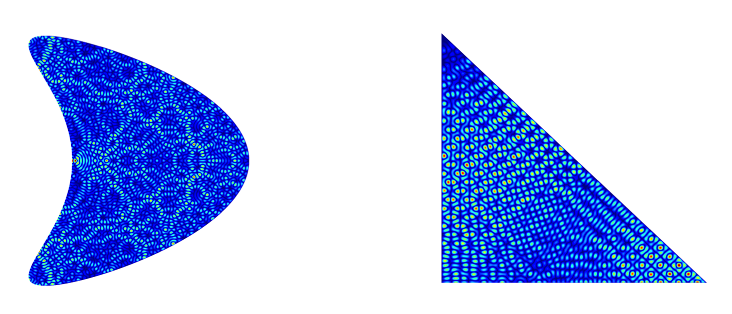
These discrete operators were used in reference [1] as important building blocks of an efficient algorithm for evaluation of eigenvalues and eigenfunctions of the Laplace operator under Zaremba boundary conditions. Figure 4 presents high-frequency Zaremba eigenfunctions obtained by means of that solver. In what follows we use these discrete operators as well as the vector of values of given functions and at the aforementioned discretization points to produce solutions of the Zaremba problem (1.1). For simplicity we rely on an -decomposition applied to the linear system to obtain a discrete approximation of the solution . Note, however, that as mentioned in Theorem 3.3, the integral equation system (3.2) is not invertible for a certain discrete set of values of (spurious resonances) that correspond to Dirichlet eigenvalues on the complementary set . A numerical methodology described in Appendix A extends applicability of the proposed solvers to all frequencies, including spurious resonances. A variety of numerical results obtained by means of the aforementioned Zaremba boundary-value solvers are presented in the following section.
7 Numerical results
This section presents results of applications of the new solvers to problems of scattering by smooth obstacles under boundary conditions of Zaremba type. This entails solution of the problem (1.1) for exterior domains and for which the right hand sides and are given by
| (7.1) |
where is the angle of incidence.
In our first experiment we apply the solver to a kite-shaped domain whose boundary is given by the parametrization
| (7.2) |
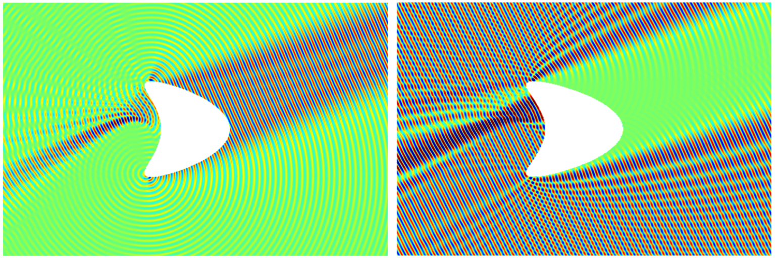
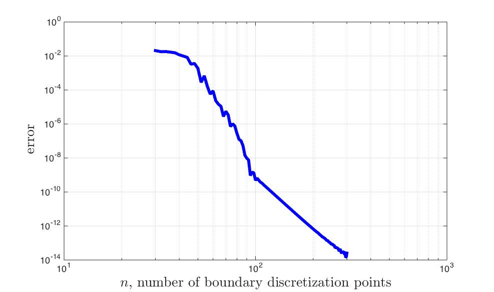
assuming the Neumann and Dirichlet boundary portions and corresponding to and its complement, respectively. Figure 5 depicts the scattered and total fields that result as a wave with wavenumber and incidence angle impinges on the object. Figure 6 demonstrates the high-order convergence results for the value of the scattered field at the point in the exterior of the domain.
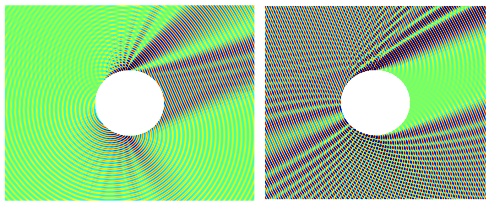
A similar example concerns scattering by the unit disc under Dirichlet and Neumann boundary conditions prescribed on the left and right halves of the disc boundary, respectively. Figure 7 displays the scattered and total fields that result as a wave with wavenumber and incidence angle impinges on the disc.
To conclude this section we present a brief comparison of the proposed solvers with one of the most efficient Zaremba solvers previously available [18, 19]. This method, which is based on iterative inverse preconditioning and which applies to a variety of singular problems, has been implemented in a numerical MATLAB package which is freely available [20]. Unfortunately, Zaremba boundary conditions are not implemented in that package. At any rate, numerical experiments suggest that the execution times required by the algorithm [20] are not as favorable as those required by the solvers proposed in this paper. Indeed, the solver [20] (which is applicable to domains with corners) required a computing time of 0.46 seconds to solve the Dirichlet problem for Helmholtz equation with wavenumber on the unit disc (whose boundary was partitioned into two Dirichlet arcs) by mean of GMRES iterations with a GMRES residual of , while a GMRES-based implementation of the FC-based solver presented in this paper runs in 0.06 seconds for the significantly more challenging Zaremba problem for the Helmholtz equation on the same domain, with the same incident wave frequency and with the same GMRES residual. (These and all other numerical results presented in this section were obtained on a single core of a 2.4 GHz Intel E5-2665 processor.) Such time differences, a factor of eight in this case, can be very significant in practice, in contexts where thousands or even tens of thousands of solutions are necessary, as is the case in inverse problems as well as in our own solution [1] of high-frequency eigenvalue problems, etc. The main reason for the difference in execution times is that even though the iterative solver [20] requires a limited number of iterations, certain iteration-dependent matrix entries occur in this solver (in view of corresponding iteration dependent discretization points it uses), which require large number of evaluations of expensive Hankel functions at each iteration, and, thus, a significant computing cost per iteration.
8 Conclusions
This paper presented, for the first time, detailed asymptotic expansions near Dirichlet-Neumann junctions for solutions of Zaremba problems on smooth two dimensional domains. By precisely accounting for the singularities of the boundary densities and kernels on the basis of Fourier-Continuation expansions, further, discretizations of high-order accuracy were obtained for relevant boundary integral operators. The resulting integral-equation solver allows for accurate and efficient approximation of the highly-singular Zaremba solutions at both the low- and high-frequency regimes.
Acknowledgments
The authors gratefully acknowledge support from AFOSR and NSF.
Appendix A Appendix: Exterior solution at interior resonances
This appendix describes an algorithm for evaluation of the solution of the problem (1.1) for an exterior domain , and for a value of that either equals or is close to an interior Dirichlet eigenvalue of the Laplace operator in the bounded set . As mentioned in Section 3 in this case the system of integral equations (3.2) does not a have a unique solution. However, the solution of the PDE is uniquely solvable for any value of .
The non-invertibility of the aforementioned continuous systems of integral equations at a wavenumber manifests itself at the discrete level in non-invertibility or ill-conditioning of the system matrix for values of close to . Therefore, for near the numerical solution of the Zaremba problems under consideration (which in what follows will be denoted by to make explicit the solution dependence on the parameter ) cannot be obtained via direct solution the linear system . As is known, however, the solutions of the continuous boundary value problem are analytic functions of for all real values of —including, in particular, for equal to any one of the spurious resonances mentioned above—and therefore, the approximate values for sufficiently far from can be used, via analytic continuation, to obtain corresponding approximations around and even at a spurious resonance .
In order to implement this strategy for a given value of it is necessary for our algorithm to possess a capability to perform two steps:
-
1.
To determine whether is “sufficiently far” from any one of the spurious resonances .
-
2a.
If is “sufficiently far” then simply invert the linear system by means of either an decomposition or the usually already available Singular Value Decomposition (which is used to determine the “distance from resonance”).
-
2b.
If is not “sufficiently far” from one of the spurious resonances , then obtain the PDE solution at by analytic continuation from solutions for values of in a neighborhood of which are “sufficiently far” from .
Here is said to be “sufficiently far” from the set of spurious resonances provided the corresponding linear system can be inverted without significant error amplifications. It has been noticed in practice [24] that the regions within which inversion is not possible are very small indeed, in such a way that analytic continuation from “sufficiently far” can be performed to the singular or nearly singular frequency with any desired accuracy. For full details in these regards see [24].
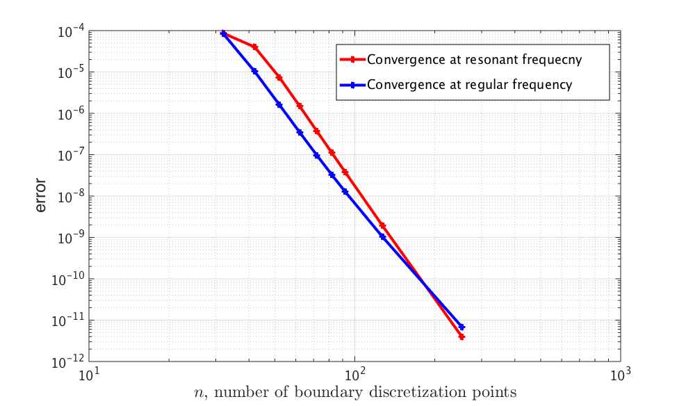
Numerical results confirming highly accurate evaluation of the PDE solution even for resonant frequencies are presented in Figure 8 for the case of the FC-based solver applied to the Zaremba boundary value problem on the unit disc. The solution errors are displayed for two frequencies: = 11 (where the solutions are obtained using an LU decomposition) and the resonant frequency (with solutions obtained by means of analytic continuation). Clearly, the proposed approach can tackle the spurious-resonance problem without difficulty.
References
- [1] Akhmetgaliyev, E., Bruno, O. P., and Nigam, N. A boundary integral algorithm for the laplace dirichlet–neumann mixed eigenvalue problem. Journal of Computational Physics 298 (2015), 1–28.
- [2] Akhmetgaliyev, E., Bruno, O. P., and Reitich, F. Integral equation solution of mixed boundary-value problems: domain smoothing and singularity resolution. In preparation.
- [3] Albin, N., and Bruno, O. P. A spectral FC solver for the compressible Navier-Stokes equations in general domains I: Explicit time-stepping. Journal of Computational Physics 230 (2011), 6248–6270.
- [4] Britt, D., Tsynkov, S., and Turkel, E. A high-order numerical method for the helmholtz equation with nonstandard boundary conditions. SIAM Journal on Scientific Computing 35, 5 (2013), A2255–A2292.
- [5] Bruno, O. P., and Lintner, S. K. Second-kind integral solvers for TE and TM problems of diffraction by open arcs. Radio Science 47, 6 (2012).
- [6] Bruno, O. P., and Lyon, M. High-order unconditionally stable FC-AD solvers for general smooth domains I. Basic elements. Journal of Computational Physics 229 (2009), 2009–2033.
- [7] Cakoni, F., Hsiao, G. C., and Wendland, W. L. On the boundary integral equation method for a mixed boundary value problem of the biharmonic equation. Complex Variables, Theory and Application: An International Journal 50, 7-11 (2005), 681–696.
- [8] Chang, D.-C., Habal, N., and Schulze, B.-W. The edge algebra structure of the zaremba problem. Journal of Pseudo-Differential Operators and Applications 5, 1 (2014), 69–155.
- [9] Colton, D. L., and Kress, R. Inverse Acoustic and Electromagnetic Scattering Theory. Springer, 1998.
- [10] Duduchava, R., and Tsaava, M. Mixed boundary value problems for the helmholtz equation in arbitrary 2d-sectors. Georgian Mathematical Journal 20, 3 (2013), 439–467.
- [11] Duduchava, R., and Tsaava, M. Mixed boundary value problems for the laplace-beltrami equations. arXiv preprint arXiv:1503.04578 (2015).
- [12] Fabrikant, V. Mixed boundary value problems of potential theory and their applications in engineering, vol. 68. Kluwer Academic Pub, 1991.
- [13] Fichera, G. Analisi esistenziale per le soluzioni dei problemi al contorno misti, relativi all’equazione e ai sistemi di equazioni del secondo ordine di tipo ellittico, autoaggiunti. Annali della Scuola Normale Superiore di Pisa-Classe di Scienze 1, 1-4 (1949), 75–100.
- [14] Fichera, G. Sul problema della derivata obliqua e sul problema misto per l’equazione di laplace. Bollettino dell’Unione Matematica Italiana 7, 4 (1952), 367–377.
- [15] Fokas, A. S. Complex variables: introduction and applications. Cambridge University Press, 2003.
- [16] Folland, G. B. Introduction to partial differential equations. 2nd edition. Princeton University Press, 1995.
- [17] Giraud, G. Problèmes mixtes et Problèmes sur des variétés closes, relativement aux équations linéaires du type elliptique. Imprimerie de l’Université, 1934.
- [18] Helsing, J. Integral equation methods for elliptic problems with boundary conditions of mixed type. Journal of Computational Physics 228:23 (2009), 8892–8907.
- [19] Helsing, J. Solving integral equations on piecewise smooth boundaries using the rcip method: a tutorial. In Abstract and Applied Analysis (2013), vol. 2013, Hindawi Publishing Corporation.
- [20] Helsing, J. Solving integral equations on piecewise smooth boundaries using the RCIP method: a tutorial. http:http://www.maths.lth.se/na/staff/helsing/Tutor/index.html, 2013.
- [21] Lorenzi, A. A mixed boundary value problem for the laplace equation in an angle (1st part). Rendiconti del Seminario Matematico della Università di Padova 54 (1975), 147–183.
- [22] Magenes, E. Sui problemi di derivata obliqua regolare per le equazioni lineari del secondo ordine di tipo ellittico. Annali di Matematica Pura ed Applicata 40, 1 (1955), 143–160.
- [23] McLean, W. C. H. Strongly elliptic systems and boundary integral equations. Cambridge university press, 2000.
- [24] Pérez-Arancibia, C., and Bruno, O. P. High-order integral equation methods for problems of scattering by bumps and cavities on half-planes. JOSA A 31, 8 (2014), 1738–1746.
- [25] Signorini, A. Sopra un problema al contorno nella teoria delle funzioni di variabile complessa. Annali di Matematica Pura ed Applicata (1898-1922) 25, 1 (1916), 253–273.
- [26] Warschawski, S. On differentiability at the boundary in conformal mapping. Proceedings of the American Mathematical Society 12, 4 (1961), 614–620.
- [27] Warschawski, S. E. On the higher derivatives at the boundary in conformal mapping. Transactions of the American Mathematical Society 38, 2 (1935), 310–340.
- [28] Wendland, W. L., Stephan, E., Hsiao, G. C., and Meister, E. On the integral equation method for the plane mixed boundary value problem of the laplacian. Mathematical Methods in the Applied Sciences 1, 3 (1979), 265–321.
- [29] Wigley, N. M. Asymptotic expansions at a corner of solutions of mixed boundary value problems. Journal of Mathematics and Mechanics 13 (1964), 549–576.
- [30] Wigley, N. M. Mixed boundary value problems in plane domains with corners. Mathematische Zeitschrift 115, 1 (1970), 33–52.
- [31] Yan, Y., Sloan, I. H., et al. On integral equations of the first kind with logarithmic kernels. University of NSW, 1988.
- [32] Zaremba, S. Sur un probleme mixte relatifa l’équation de laplace. Bulletin de l’Académie des sciences de Cracovie, Classe des sciences mathématiques et naturelles, série A (1910), 313–344.