Conditional decoupling of random interlacements

Abstract

We prove a conditional decoupling inequality for the model of random interlacements in dimension $d\geq 3$: the conditional law of random interlacements on a box (or a ball) $A_{1}$ given the (not very “bad”) configuration on a “distant” set $A_{2}$ does not differ a lot from the unconditional law. The main method we use is a suitable modification of the soft local time method of [13], that allows dealing with conditional probabilities.

Keywords and phrases. Random interlacements, stochastic domination, soft local time
MSC 2010 subject classifications. Primary 60K35; Secondary 60G50, 82C41.

1 Introduction

Random interlacements were introduced by Sznitman in [17], to model the trace of the simple random walk on the discrete torus $\mathbb{Z}_{n}^{d}:=\mathbb{Z}^{d}/n\mathbb{Z}^{d}$ or the discrete cylinder $\mathbb{Z}\times\mathbb{Z}^{d-1}$, in dimension $d\geq 3$. Detailed treatments and reviews of recent results can be found in the recent books [4, 6, 19]. Loosely speaking, the model of random interlacements in $\mathbb{Z}^{d}$, $d\geq 3$, is a stationary Poissonian soup of bi-infinite simple random walk trajectories on the integer lattice. There is a parameter $u>0$ entering the intensity measure of the Poisson process, the larger $u$ is the more trajectories are thrown in. The sites of $\mathbb{Z}^{d}$ that are not touched by the trajectories constitute the vacant set $\mathcal{V}^{u}$, and the union of all trajectories constitutes the interlacement set $\mathcal{I}^{u}=\mathbb{Z}^{d}\setminus\mathcal{V}^{u}$. The random interlacements are constructed simultaneously for all $u>0$ in such a way that $\mathcal{I}^{u_{1}}\subset\mathcal{I}^{u_{2}}$ if $u_{1}<u_{2}$. In fact, the law of the vacant set at level $u$ can be uniquely characterized by the following identity:

(1.1) $$\mathbb{P}[A\subset\mathcal{V}^{u}]=\exp\big{(}-u\operatorname{cap}(A)\big{)},$$

where $\operatorname{cap}(A)$ is the capacity of a finite set $A\subset\mathbb{Z}^{d}$. Informally, the capacity measures how “big” is the set from the point of view of the walk, see Section 6.5 of [11] for formal definitions, or Section 2 below.

The model of random interlacements naturally has more independence built in than just one random walk on the torus or the cylinder (because on a fixed set one observes traces of independent trajectories). Still, the analysis of random interlacements is difficult because of the long-range dependencies present there. For example, in $(1.68)$ from [17] we can see that

(1.2) $$\operatorname{Cov}({{1}}_{x\in\mathcal{I}^{u}},{{1}}_{y\in\mathcal{I}^{u}})\sim\frac{c_{d}u}{\|x-y\|^{d-2}}\quad\text{ as }\quad\|x-y\|\to\infty,$$

which means that the “degree of dependence” decreases polynomially in the distance.

Naturally, one is interested in “decoupling” the events supported on distant regions; that is, to argue that they are approximately independent to a certain degree. One possible approach to quantify that degree is the following: given finite sets $A_{1},A_{2}~{}\subset~{}\mathbb{Z}^{d}$ and functions $f_{1}:\{0,1\}^{A_{1}}\to[0,1]$ and $f_{2}:\{0,1\}^{A_{2}}\to[0,1]$ depending on the interlacements set intersected with $A_{1}$ and $A_{2}$ respectively, we have

(1.3) $$\operatorname{Cov}_{u}(f_{1},f_{2})\leq c_{d}u\frac{\operatorname{cap}(A_{1})\operatorname{cap}(A_{2})}{\operatorname{dist}(A_{1},A_{2})^{d-2}},$$

as proved in formula $(2.15)$ of [17], see also $(8.1.1)$ in [6]. However, the polynomial error term in (1.3) can complicate one’s life in many applications (and, e.g. in the case when the diameters of these sets are of the same order as the distance between them, (1.3) is simply of no use); on the other hand, while (1.3) can be improved to some degree [2], the error term there should always be at least polynomial, as (1.2) shows. To circumvent this difficulty, one first may note that usually the “interesting” events/functions are monotone (i.e., increasing or decreasing). For e.g. increasing events, we know that their probabilities increase as the parameter $u$ increases. Note also that the FKG inequality (see [21], Theorem $3.1$) gives us

(1.4) $$\mathbb{E}^{u}[g_{1}g_{2}]\geq\mathbb{E}^{u}[g_{1}]\mathbb{E}^{u}[g_{2}],$$

for any increasing functions $g_{1,2}$ with finite second moments. To complement the FKG inequality, we use sprinkling, i.e., we slightly change the intensity of random interlacements in order to decrease the error term; this approach was used in [17] and [18]. Then, in particular, in [13] it was proved that

(1.5) $$\mathbb{E}^{u}[f_{1}f_{2}]\leq\mathbb{E}^{(1+\varepsilon)u}[f_{1}]\mathbb{E}^{(1+\varepsilon)u}[f_{2}]+c_{d}(r+s)^{d}\exp(-c_{d}^{\prime}\varepsilon^{2}us^{d-2});$$

with $f_{1}:\{0,1\}^{A_{1}}\to[0,1]$ and $f_{2}:\{0,1\}^{A_{2}}\to[0,1]$ both increasing functions in the interlacements set, $r=\min(\operatorname{diam}(A_{1}),\operatorname{diam}(A_{2}))$, and $s=\operatorname{dist}(A_{1},A_{2})$. The same bound was also obtained for decreasing functions.

It is important to observe, however, that the decoupling in the above form may not always be useful for one’s needs. Intuitively, one is tempted to understand inequalities like (1.3) as “what happens in one set does not influence a lot what happens in the other set”. Now, consider the following situation. Suppose that on top of the random interlacements we have some additional stochastic process (e.g., a random walk) that “explores” the interlacement set in some way. Assume that this process has already explored the interlacements in a given area, revealing a lot of information about it; think, for definiteness, that it simply revealed the interlacement set exactly. The probability of a particular configuration of the interlacement set is usually very small; so, (1.3) (even (1.5)!) will blow up when one divides by that probability, because of the error term. In fact, in the end of Section 2 we discuss a particular model of the random walk on the interlacement set, where our main results turn out to be useful.

This justifies the need for conditional decoupling, i.e., show that, given the configuration on some set, the law of the interlacement configuration on a distant set is still in some sense close to the unconditional law. This is what we are doing in this paper. To prove our results, the main method we use is a suitable modification (that allows dealing with conditional probabilities) of the soft local time method of [13]. We hope that this modification will be useful in other contexts, for instance, for dealing with the decoupling properties of the loop measures [3].

Another important observation is the following. There are strong connections between random interlacements and the Gaussian free field, see e.g. [19, 20]. In particular, there are decoupling inequalities similar to (1.3) and (1.5) for the Gaussian free field as well, see [12]. Notice, however, that the decoupling-with-sprinkling result for the Gaussian free field (Theorem $1.2$ of [12]) is already conditional (the unconditional decoupling is obtained as a simple consequence, just by integration). On the other hand, note that the error terms in the conditional decoupling in the main result of this paper (Theorem 2.1) are much worse than that of (1.5); related to this is the fact that in the conditional setting the minimal distance between sets that permits the result to work is much bigger. A comparison with the situation for the Gaussian free field suggests that, hopefully, there is still much room for improvement for the conditional decoupling for random interlacements.

2 Definitions, notations and results

In this section we will introduce the basic definitions, conventions and notation used in this paper. We will then be able to state our main result. We start by stating our convention regarding constants: $c$, $c^{\prime}$, $c_{1}$, $c_{2}$, $c_{3}$,$\dots$ are always defined as strictly positive constants depending only on the dimension $d$. Constants can also change value from line to line, unless when the text explicitly states to the contrary.

We let $\|\cdot\|$ and $\|\cdot\|_{\infty}$ denote the Euclidean and $\ell_{\infty}$ norms in $\mathbb{Z}^{d}$ respectively. For $x,y\in\mathbb{Z}^{d}$, we also let $\operatorname{dist}(x,y)\equiv\|x-y\|$. We say that two vertices $x,y\in\mathbb{Z}^{d}$ are neighbors when $\|x-y\|=1$, this notion introduces the usual nearest-neighbor graph structure in $\mathbb{Z}^{d}$. For $x\in\mathbb{Z}^{d}$ and $r\in\mathbb{R}_{+}$, we define

$$B(x,r):=\big{\{}y\in\mathbb{Z}^{d};\|y-x\|\leq r\big{\}},$$

the discrete ball in the Euclidean norm centered on $x$ with radius $r$, and

$$B_{\infty}(x,r):=\big{\{}y\in\mathbb{Z}^{d};\|y-x\|_{\infty}\leq r\big{\}},$$

the discrete ball in the $\ell_{\infty}$-norm centered on $x$ with radius $r$. Given a set $A\subseteq\mathbb{Z}^{d}$ we denote by

$$A^{C}:=\{x\in\mathbb{Z}^{d};x\notin A\}$$

its complement and by

$$\partial A:=\big{\{}x\in A;\text{ there exists $y\in A^{C}$ such that $\|x-y\|=1$}\big{\}}$$

its (internal) boundary.

For any set $Z$ and any two functions $f,g:Z\mapsto\mathbb{R}$, we write $f(z)\asymp g(z)$ to denote the fact that there exist two strictly positive constants, $c_{1}$ and $c_{2}$, such that $c_{1}f(z)\leq g(z)\leq c_{2}f(z)$ for all $z\in Z$. When $Z$ is equal to $\mathbb{R}$ we say that $f(z)=o(g(z))$ when $\frac{f(z)}{g(z)}$ goes to $0$ as $z\rightarrow\infty$.

Given $x\in\mathbb{Z}^{d}$, we let $\mathbb{P}_{x}$ denote the probability measure associated with the simple random walk in $\mathbb{Z}^{d}$ started at $x$. We will also let $(X_{k},k\geq 0)$ denote the simple random walk process in $\mathbb{Z}^{d}$. Given a set $A\subset\mathbb{Z}^{d}$, we define the entrance time for the set $A$

$$H_{A}:=\inf\big{\{}k\geq 0;X_{k}\in A\big{\}}.$$

We also let the hitting time for $A$ be defined as

$$\tilde{H}_{A}:=\inf\big{\{}k\geq 1;X_{k}\in A\big{\}}.$$

When $A$ is finite we denote its harmonic measure by

$$e_{A}(x)={{1}}_{x\in A}\mathbb{P}_{x}\big{[}\tilde{H}_{A}=\infty\big{]}\text{ for $x\in\mathbb{Z}^{d}$}.$$

We are then able to define the capacity of the set $A$

$$\operatorname{cap}(A):=\sum_{x\in A}e_{A}(x),$$

and the normalized harmonic measure

$$\overline{e}_{A}(x):=e_{A}(x)\operatorname{cap}(A)^{-1}.$$

We now write down the definition of the Green’s function for the simple random walk in $\mathbb{Z}^{d}$: for $x,y\in\mathbb{Z}^{d}$, we let

$$G(x,y):=\sum_{k\geq 0}\mathbb{P}_{x}\big{[}X_{k}=y\big{]}.$$

Theorem $1.5.4$ of [10] provides us with the following estimate on the Green’s function:

(2.1) $$G(x,y)\asymp\frac{1}{1+\|x-y\|^{d-2}}.$$

Let us briefly discuss the definition of the measure associated with the random interlacements process intersected with a given finite set $A\subset\mathbb{Z}^{d}$. Assume we have constructed a probability space where, for every $i\geq 1$, there exists a simple random walk process $(X^{(i)}_{k},k\geq 0)$ with starting distribution given by $\overline{e}_{A}(\cdot)$, and such that $(X^{(i)}_{k},k\geq 0)$ is independent from $(X^{(j)}_{k},k\geq 0)$ for $i\neq j$. We also assume that in this space we can construct an independent Poisson process $(J_{u})_{u\geq 0}$ on the positive real line with intensity $\operatorname{cap}(A)$. The law of the random interlacements process $(\mathcal{I}^{u})_{u\geq 0}$ intersected with the set $A$ can then be characterized by

(2.2) $$(\mathcal{I}^{u}\cap A)_{u\geq 0}\stackrel{{\scriptstyle\tiny d}}{{=}}\Big{(}A\cap\bigcup_{i\leq J_{u}}\bigcup_{k\geq 0}X_{k}^{(i)}\Big{)}_{u\geq 0},$$

as can be seen in [17], Proposition $1.3$, or in the paragraph before $(2.6)$ in [5]. This definition gives rise to compatible measures in the following sense: Given two finite sets $K_{1}\subset K_{2}\subset\mathbb{Z}^{d}$, we have that $((\mathcal{I}^{u}\cap K_{2})_{u\geq 0})\cap K_{1}$ has the same law as $(\mathcal{I}^{u}\cap K_{1})_{u\geq 0}$.

To state our main result, we need more definitions.

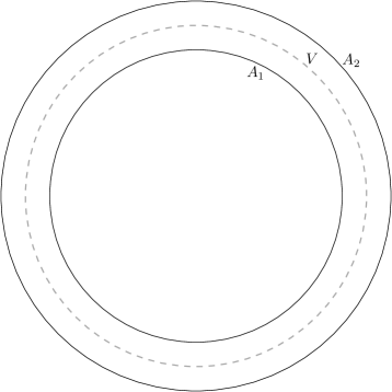
Figure 1: Definition of the sets $A_{1}^{\tiny\Circle}$, $A_{2}^{\tiny\Circle}$ and $V^{\tiny\Circle}$.

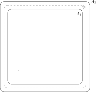
Figure 2: Definition of the sets $A_{1}^{\tiny\Square}$, $A_{2}^{\tiny\Square}$ and $V^{\tiny\Square}$.

Let $r>0$ be sufficiently big, and let $s:=s(r)>0$, with $s=o(r)$. We define $A_{1}^{\tiny\Circle}:=A_{1}^{\tiny\Circle}(r)$ to be the discrete ball of radius $r$, that is

$$A_{1}^{\tiny\Circle}:=\{x_{1}\in\mathbb{Z}^{d};\operatorname{dist}(x_{1},0)<r\}.$$

We also define $A_{1}^{\tiny\Square}:=A_{1}^{\tiny\Square}(r,s)$ to be a $d$-dimensional discrete ‘hypercube’ with edge length $r$ and a smoothed frontier such that for every point $x_{1}\in\partial A_{1}$ there exists a discrete Euclidean ball $B_{x_{1}}$ of radius $s$ contained in $A_{1}$ such that $B_{x_{1}}\cap A_{1}^{C}=x_{1}$. More precisely, we let $\mathfrak{H}_{r-s}$ be a discrete $d$-dimensional hypercube with edge length $r-s$ contained in $\mathbb{Z}^{d}$ and define

$$A_{1}^{\tiny\Square}:=\{x_{1}\in\mathbb{Z}^{d};\operatorname{dist}(x_{1},\mathfrak{H}_{r-s})\leq s\}.$$

We refer the reader to [13], Section $8$, to see that $A_{1}^{\tiny\Square}$ possesses the desired properties. Note that, since $s=o(r)$, the diameter of $A_{1}^{\tiny\Square}$ is of order $r$.

We then define $A_{2}^{\tiny\Circle}:=A_{2}^{\tiny\Circle}(r,s)$ to be the set of points that are at least at distance $2s$ from $A_{1}^{\tiny\Circle}$:

$$A_{2}^{\tiny\Circle}:=\{x_{1}\in\mathbb{Z}^{d};\operatorname{dist}(x_{1},x_{2})>2s\text{ for every $x_{2}\in$}A_{1}^{\tiny\Circle}\}.$$

We finally define $V^{\tiny\Circle}:=V^{\tiny\Circle}(r,s)$ to be the boundary set

$$V^{\tiny\Circle}:=\partial\{x_{1}\in\mathbb{Z}^{d},\operatorname{dist}(x_{1},x_{2})\leq s\text{ for some $x_{2}\in$}A_{1}^{\tiny\Circle}\},$$

separating $A_{1}^{\tiny\Circle}$ from $A_{2}^{\tiny\Circle}$. We analogously define $A_{2}^{\tiny\Square}(r,s)$ and $V^{\tiny\Square}(r,s)$. It will also be useful to define the $d$-dimensional hypercube $\mathfrak{H}_{r+2s}$ of edge length $r+2s$ concentric with $\mathfrak{H}_{r-s}$, which will essentially be the unsmoothed version of $(A_{2}^{\tiny\Square})^{C}$.

When there is no risk of confusion, or when the arguments presented work for both balls and smoothed hypercubes (which will be often so), we will omit the super-indexes $\tiny\Circle,\tiny\Square$.

Since $s=o(r)$, we have

$$\operatorname{cap}(V)=\operatorname{cap}(A_{2})(1+o(1))=\operatorname{cap}(A_{1})(1+o(1)),$$

and also, by Proposition $2.2.1$ and equation $(2.16)$ of [10],

(2.3) $$\operatorname{cap}(V)\asymp r^{d-2}.$$

We will now state our main result. Heuristically, it says the following: Let $s$ be bounded from below by a polynomial of $r$ with a explicit given coefficient (strictly smaller than $1$, depending only on the dimension $d$ and whether $A_{1}$ is a ball or a smoothed hypercube). Let $A_{3}$ be a subset of $A_{2}$ with finite boundary, that is, $A_{3}$ is either finite or has finite complement. If we pay a stretched exponentially small price (in $s$) to guarantee that the interlacements configuration of $\mathcal{I}^{u}\cap A_{3}$ is not too weird, then the distribution of $I^{u}\cap A_{1}$ conditioned on this configuration is well approximated by the unconditional distribution, with high probability ($1$ minus a stretched exponential function of $s$).

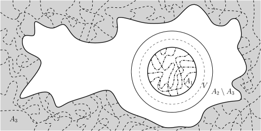
Figure 3: Our main result says that if the interlacements configuration in a set $A_{3}\subseteq A_{2}$ is not too weird, that is, it does not belong to a set with stretched exponentially small probability (in $s$, as $s\rightarrow\infty$), then with high probability ($1$ minus stretched exponential in $s$) the distribution of the interlacements set intersected with $A_{1}$ conditioned on the state of $\mathcal{I}^{u}\cap A_{3}$ can be well approximated by the unconditional distribution.

Theorem 2.1.

Let the real numbers $b_{A_{1}^{\tiny\Circle}},b_{A_{1}^{\tiny\Square}}$ be such that

(2.4) $$1\leq b_{A_{1}^{\tiny\Circle}}<\frac{2d-2}{d},$$

(2.5) $$1\leq b_{A_{1}^{\tiny\Square}}<\frac{4d-4}{3d-2}.$$

Then, define

(2.6) $$a_{A_{1}^{\tiny\Circle}} =2d-2-db_{A_{1}^{\tiny\Circle}}>0,$$

(2.7) $$a_{A_{1}^{\tiny\Square}} =4d-4-3db_{A_{1}^{\tiny\Square}}+2b_{A_{1}^{\tiny\Square}}>0.$$

From now on we will again omit the indexes $\tiny\Circle,\tiny\Square$. Recall that $r$ is of the same order as the diameter of $A_{1}$, and that $s$ has the same order as the distance between $A_{1}$ and $A_{2}$. Assume $r\asymp s^{b_{A_{1}}}$, let $s$ be sufficiently big. Let $\varepsilon>0$ be smaller then $1/4$. Let $A_{3}$ be a subset of $A_{2}$ such that $|\partial A_{3}|<\infty$. Define $\mathcal{I}^{u}_{A_{j}}:=\mathcal{I}^{u}\cap A_{j}$, for $j=1,2,3$.

Then there are positive constants $c,c^{\prime}$ depending only on the dimension $d$, and a measurable (according to the random interlacements $\sigma$-field) set $\mathcal{G}\in\{0,1\}^{A_{3}}$ such that

$$\mathbb{P}^{u}\big{[}\mathcal{I}^{u}_{A_{3}}\in\mathcal{G}\big{]}\geq 1-\exp\Big{(}-\frac{c^{\prime}}{2}\varepsilon^{2}us^{a_{A_{1}}}\Big{)},$$

and for any increasing function $f$ on the interlacements set intersected with $A_{1}$, with $\sup|f|<M$, we have

$$\big{(}\mathbb{E}f(\mathcal{I}^{u(1-\varepsilon)}_{A_{1}})-cM\exp\big{(}-c^{\prime}\varepsilon^{2}us^{a_{A_{1}}}\big{)}\big{)}{{1}}_{\mathcal{I}^{u}_{A_{3}}\in\mathcal{G}}\leq\mathbb{E}\big{(}f(\mathcal{I}^{u}_{A_{1}})\mid\mathcal{I}^{u}_{A_{3}}\big{)}{{1}}_{\mathcal{I}^{u}_{A_{3}}\in\mathcal{G}}$$

(2.8) $$\leq\big{(}\mathbb{E}f(\mathcal{I}^{u(1+\varepsilon)}_{A_{1}})+cM\exp\big{(}-c^{\prime}\varepsilon^{2}us^{a_{A_{1}}}\big{)}\big{)}{{1}}_{\mathcal{I}^{u}_{A_{3}}\in\mathcal{G}}.$$

We also obtain a result analogous to Theorem 2.1, but this time we allow the sprinkling factor to be arbitrarily big. This decreases the “precision” (in the result below, $\mathbb{E}f(\mathcal{I}^{u+u^{\prime}}_{A_{1}})$ can be very different from $\mathbb{E}f(\mathcal{I}^{u}_{A_{1}})$), but, in compensation, the size of the complement of the “good” set as well as the “error term” become smaller.

Theorem 2.2.

Let $u^{\prime}>u>0$. We use the same definitions as Theorem 2.1. There are positive constants $c,c^{\prime}$ depending only on the dimension $d$, and a measurable (according to the random interlacements $\sigma$-field) set $\mathcal{G}_{u^{\prime}}\in\{0,1\}^{A_{3}}$ such that

$$\mathbb{P}^{u}\big{[}\mathcal{I}^{u}_{A_{3}}\in\mathcal{G}_{u^{\prime}}\big{]}\geq 1-\exp\Big{(}-c^{\prime}u^{\prime}s^{a_{A_{1}}}\Big{)},$$

and for any increasing function $f$ on the interlacements set intersected with $A_{1}$, with $\sup|f|<M$, we have

(2.9) $$\mathbb{E}\big{(}f(\mathcal{I}^{u}_{A_{1}})\mid\mathcal{I}^{u}_{A_{3}}\big{)}{{1}}_{\mathcal{I}^{u}_{A_{3}}\in\mathcal{G}_{u^{\prime}}}\leq\big{(}\mathbb{E}f(\mathcal{I}^{u+u^{\prime}}_{A_{1}})+cM\exp\big{(}-c^{\prime}u^{\prime}s^{a_{A_{1}}}\big{)}\big{)}{{1}}_{\mathcal{I}^{u}_{A_{3}}\in\mathcal{G}_{u^{\prime}}}.$$

Remark 2.3.

We have to explain why we need to consider $A_{3}\subset A_{2}$. Indeed, at first sight it seems that conditioning on a configuration on $A_{3}$ does not add generality to our results, since any fixed configuration on $A_{3}$ corresponds to a set of configurations on $A_{2}$. However, the problem with always setting $A_{3}=A_{2}$ is the following: the “exceptional set” $\mathcal{G}^{c}$ will then be supported on the whole $A_{2}$, and this can be inconvenient for applications. For example, assume that we successively apply the conditional decoupling results to a process (such as the one of Section 2.1) that “explores” the interlacement environment. If that process has explored only a finite chunk of $A_{2}$, we would not be able to say if the configuration is “good” (i.e., belongs to $\mathcal{G}$) by only observing that finite chunk. This would force us to condition on the (configuration on the) whole $A_{2}$, which would mean that a subsequent application of a conditional decoupling may be difficult, since we already “revealed” some information about the configuration on a set which is “too big” (i.e., when we apply the decoupling result for the next time, the “new” $A_{1}$ may be inside the “previous” $A_{2}$)

Remark 2.4.

In the course of the proof of the above theorems we actually prove a stronger result: the same conditional decoupling inequality holds true if we replace the sets $\mathcal{I}^{u}_{A_{1}}\subset A_{1}$ and $\mathcal{I}^{u}_{A_{3}}\subset A_{3}$ by sets of random walk excursions in $A_{1}$ and $A_{3}$ (we also have to replace the function $f$ by an increasing function on the set of excursions). That is, the conditional decoupling continues to work when we replace the ranges of the excursions (which constitute the random interlacements set) by the actual excursions themselves. We chose to state the results in the above manner for the sake of clarity and brevity. Note that this remark also applies to the decoupling obtained by Popov and Teixeira in [13].

Remark 2.5.

The above theorems can be proved in the same way if we replace the smoothed hypercube $A_{1}^{\tiny\Square}$ by a smoothed version of a box $[0,a_{1}]\times\dots\times[0,a_{d}]$, with $c^{-1}r<a_{i}<cr$ for all $i=1,\dots,d$, and some constant $c>1$, and then replace the sets $A_{2}^{\tiny\Square}$ and $V^{\tiny\Square}$ accordingly. We chose to prove the theorems for $A_{1}^{\tiny\Square}$ only to simplify the notation. We also note that we prove the theorem for both balls and boxes because the error term obtained in the decoupling for balls is much smaller than the error obtained in the decoupling for boxes, but at the same time the decoupling between boxes tends to be more useful because boxes cover the space in a much more efficient manner.

Remark 2.6.

For $d=3$, the only way to obtain an exponentially small (instead of a stretched exponentially small) error term in equations (2.1) and (2.9) is to allow the distance $\sim s$ between the sets $A_{1}$ and $A_{2}$ to be of the same order of the minimal diameter $\sim~{}r$.

Here is an overview of the paper. In Subsection 2.1, we discuss an application of some of our results. In Section 3 we recall the soft local times technique. In Section 4 we show how we simulate the interlacements set $\mathcal{I}^{u}_{A_{1}}$ conditioned on the information given by $\mathcal{I}^{u}_{A_{2}}$ using a suitable version of the soft local times method. Finally, in Section 5, we prove the main theorem using a large deviations estimate for the soft local times associated with $\mathcal{I}^{u}_{A_{1}}$. The Appendix is then used to collect and derive the technical estimates we need.

2.1 An application: biased random walk on the interlacement set

Let $G$ be some (possibly random) subset of $\mathbb{Z}^{d}$, $d\geq 2$. Fix a parameter $\beta>0$, which accounts for the bias; also, fix some non-zero vector $\ell\in\mathbb{Z}^{d}$. Let us define the conductances on the edges of $\mathbb{Z}^{d}$ in the following way:

$$\mathcal{C}(x,y)=\begin{cases}e^{\beta(x+y)\cdot\ell},&\text{if $x,y$ are neighbors and belong to $G$},\\ 0,&\text{otherwise},\end{cases}$$

and we call the collection of all conductances $\omega=\big{\{}\mathcal{C}(x,y),x,y\in\mathbb{Z}^{d}\big{\}}$ the random environment. Consider a random walk $(X_{n},n\geq 0)$ in this environment of conductances; i.e., its transition probabilities are given by

$$P^{\omega}[X_{n+1}=y\mid X_{n}=x]=\frac{\mathcal{C}(x,y)}{\sum_{z}\mathcal{C}(x,z)}$$

(the superscript in $P^{\omega}$ indicates that we are dealing with the “quenched” probabilities, i.e., when the underlying random graph / conductancies are already fixed).

There have been significant interest towards this model in recent years, mainly in the case when $G$ is the infinite cluster of supercritical Bernoulli percolation model, see e.g. [1, 16, 7]. In particular, one remarkable fact is the following: the walk is ballistic (transient and with positive speed) in the direction of the drift if $\beta>0$ is small enough; however, it moves only sublinearly fast (its displacement is only of order $t^{a}$ by time $t$ with $a\in(0,1)$, as proved in [8]) for large values of $\beta$.

In the work [9] the case $G=\mathcal{I}^{u}$ was considered. It turned out that in dimension $d=3$, for any value of $\beta>0$, although still transient in the direction of the drift, the walk is not only sub-ballistic, but has also sub-polynomial speed, in the sense that its distance to the origin grows slower than $t^{\varepsilon}$ for any $\varepsilon>0$. This is also in contrast with the result that the walk on $\mathcal{I}^{u}$ without any drift is diffusive (so, loosely speaking, its “speed” is $\sqrt{t}$), as shown in [14].

We will not describe all the details of [9] here, but the main idea is the following. As in the case of the biased walk on the infinite percolation cluster, to prove zero speed one needs to show that the walk frequently gets caught in traps. These traps are “dead ends” of the environment looking in the direction of the bias, see Figure 4.

Figure 4: A trap for the random walk on the interlacement set (on this picture, the bias is directed along the first coordinate vector). Only the interlacements are shown; the trajectory of the RWRE $X$ is not present on the picture.

When the walk enters such a trap, the bias prevents it from goint out, so there is a good chance that the walk will spend quite a lot of time there, and this effectively leads to zero speed. Now, the crucial fact is that, specifically in three dimensions, it is much cheaper to have a trap in the interlacement set than in the (Bernoulli) percolation cluster. Indeed, it is possible to show that the capacity of the dotted set on Figure 4 is of order $\frac{\ln t}{\ln\ln t}$ for any fixed $\alpha<1$. The formula (1.1) then shows that having a trap as above has only a subpolynomial (in $t$) cost; also, it turns out that “forcing” a trajectory to create a “dead end” as shown on the picture is not too costly as well.

So, when the walk advances in the direction of the bias, from time to time it will encounter a trap and be trapped. However, to make such an argument rigorous, one has to face the following difficulty. When the walk already explored some parts of the environment and then came to an unexplored area, we can no longer use (1.1) to estimate the probability that there is a trap in front of it, due to the lack of independence. It is here that the conditional decoupling enters the scene: it is possible to use the main results of this paper to show that probability of having a trap in front of the particle (when it comes to an unexplored area) is not very small. As mentioned above, the detailed argument can be found in [9].

3 Soft local times

In the present section we describe the technique introduced in [13], the so called Soft Local Times method. This method essentially allows us to simulate any number of random variables taking values in a state space $\Sigma$ using a realization of a Poisson point process in $\Sigma\times\mathbb{R}_{+}$.

Let $\Sigma$ be a locally compact Polish metric space, and let $\mathcal{B}(\Sigma)$ be its Borel $\sigma$-algebra. Let $\mu$ be a Radon measure over $\mathcal{B}(\Sigma)$, so that every compact set has finite $\mu$-measure.

Such measure space $(\Sigma,\mathcal{B}(\Sigma),\mu)$ is the usual setup for the construction of a Poisson point process on $\Sigma$. We consider the space of Radon point measures in $\Sigma\times\mathbb{R}_{+}$

(3.1) $$L=\Big{\{}\eta=\sum_{\lambda\in\Lambda}\delta_{(z_{\lambda},v_{\lambda})};z_{\lambda}\in\Sigma,v_{\lambda}\in\mathbb{R}_{+}\text{ and }\eta(K)<\infty\text{ for all compact $K$}\Big{\}},$$

endowed with the $\sigma$-algebra generated by the evaluation maps

$$\eta\mapsto\eta(D),\phantom{*}D\in\mathcal{B}(\mathbb{R}_{+})\otimes\mathcal{B}(\Sigma).$$

We are then able to construct a Poisson point process $\eta$ in the space $(L,\mathcal{D},\mathbb{Q})$ with intensity measure given by $\mu\otimes\mathrm{d}v$, where $\mathrm{d}v$ is the Lebesgue measure on $\mathbb{R}_{+}$, see [15], Proposition $3.6$ on p.$130$.

The next proposition, originally seen in [13], is at the core of the soft local times argument.

Proposition 3.1.

Let $g:\Sigma\to\mathbb{R}_{+}$ be a measurable function with $\int g(z)\mu(\mathrm{d}z)=1$. For $\eta=\sum_{\lambda\in\Lambda}\delta_{(z_{\lambda},v_{\lambda})}\in L$, we define

(3.2) $$\xi=\inf\{t\geq 0;\text{ there exists $\lambda\in\Lambda$ such that $tg(z_{\lambda})\geq v_{\lambda}$}\}.$$

Then under the law $\mathbb{Q}$ of the Poisson point process $\eta$,

1. there exists a.s. a unique $\hat{\lambda}\in\Lambda$ such that $\xi g(z_{\hat{\lambda}})=v_{\hat{\lambda}}$,

2. $(z_{\hat{\lambda}},\xi)$ is distributed as $g(z)\mu(dz)\otimes\mathop{\mathrm{Exp}}(1)$,

3. $\eta^{\prime}:=\sum_{\lambda\neq\hat{\lambda}}\delta_{(z_{\lambda},v_{\lambda}-\xi g(z_{\lambda}))}$ has the same law as $\eta$ and is independent of $(\xi,\hat{\lambda})$.

The proof is remarkably simple, mainly relying on the independence of a Poisson process in disjoint sets, and can be seen in the original paper.

With the above proposition we are able to simulate as many random variables as we want:

Figure 5: An example showing the definition below. Under mild conditions we are able to use Proposition 3.1 to simulate a sequence of random variables over $\Sigma$.

Let $X_{1},X_{2},\dots,X_{n}$ be random variables on $\Sigma$ such that $X_{1}$’s distribution is absolutely continuous with respect to $\mu$ and, for all $i=2,\dots,n$ the probability measure generated by $X_{i}$, conditioned on on the values taken by $X_{1},\dots,X_{i-1}$, is absolutely continuous with respect to $\mu$. Using the process $\eta$ constructed above, we define

(3.3) $$g_{1}:\Sigma\mapsto\mathbb{R}_{+}\text{, the density function of $X_{1}$ with respect to $\mu$,}$$

$$\xi_{1}:=\inf\big{\{}t\geq 0;\text{ there exists $\lambda\in\Lambda$ such that $tg_{1}(z_{\lambda})\geq v_{\lambda}$}\big{\}},$$

$$G_{1}(z):=\xi_{1}\;g_{1}(z),\text{ for $z\in\Sigma$,}$$

$$(z_{\lambda_{1}},v_{\lambda_{1}})\text{, the unique pair in $\{(z_{\lambda},v_{\lambda})\}_{\lambda\in\Lambda}$ with $G_{1}(z_{\lambda_{1}})=v_{\lambda_{1}}$.}$$

We now define $g_{2}:\Sigma\mapsto\mathbb{R}_{+}$ to be the density of $X_{2}$ conditioned on the event $\{X_{1}=z_{\lambda_{1}}\}$. Using the fact that $\eta_{1}:=\sum_{\lambda\neq{\lambda_{1}}}\delta_{(z_{\lambda},v_{\lambda}-\xi_{1}g_{1}(z_{\lambda}))}$ has the same law as $\eta$ and is independent from $(\xi_{1},{\lambda_{1}})$ we define

(3.4) $$\xi_{2}:=\inf\big{\{}t\geq 0;\text{ there exists $\lambda\in\Lambda$ such that $tg_{2}(z_{\lambda})+G_{1}(z_{\lambda})\geq v_{\lambda}$}\big{\}},$$

$$G_{2}(z):=\xi_{2}\;g_{2}(z)+G_{1}(z),\text{ for $z\in\Sigma$,}$$

$$(z_{\lambda_{2}},v_{\lambda_{2}})\text{, the unique pair in $\{(z_{\lambda},v_{\lambda})\}_{\lambda\in\Lambda}$ with $G_{2}(z_{\lambda_{2}})=v_{\lambda_{2}}$.}$$

Then, recursively, for $1\leq k\leq n$ we define $g_{k}:\Sigma\mapsto\mathbb{R}_{+}$ to be the density function of $X_{k}$ conditioned on the event $\{X_{1}=z_{\lambda_{1}},\dots,X_{k-1}=z_{\lambda_{k-1}}\}$,

(3.5) $$\xi_{k}:=\inf\big{\{}t\geq 0;\text{ there exists $\lambda\in\Lambda$ such that $tg_{k}(z_{\lambda})+G_{k-1}(z_{\lambda})\geq v_{\lambda}$}\big{\}},$$

$$G_{k}(z):=\xi_{k}\;g_{k}(z)+G_{k-1}(z),\text{ for $z\in\Sigma$,}$$

$$(z_{\lambda_{k}},v_{\lambda_{k}})\text{, the unique pair in $\{(z_{\lambda},v_{\lambda})\}_{\lambda\in\Lambda}$ with $G_{k}(z_{\lambda_{k}})=v_{\lambda_{k}}$.}$$

We refer to Figure 5. Using Proposition 3.1 together with the above construction, we are able to state the following proposition:

Proposition 3.2.

The vector $(z_{\lambda_{1}},\dots,z_{\lambda_{n}})$ has the same law as $(X_{1},\dots,X_{n})$.

We call the function $G_{n}(z)$ the soft local time of the vector $(X_{1},\dots,X_{n})$ up to time $n$ with respect to the measure $\mu$, or more usually simply the soft local time. If $T$ is a stopping time with respect to the canonical filtration generated by the variables $X_{i}$, it is simple to define $G_{T}(z)$, the soft local time up to time $T$.

Note that by controlling the value of the soft local times function we will automatically control the values our random variables take, as the next corollary summarizes:

Corollary 3.3.

For any measurable function $h:\Sigma\to\mathbb{R}_{+}$ we have, using the same notation as above,

(3.6) $$\mathbb{Q}\Big{[}\{z_{1},\dots,z_{T}\}\subseteq\{z_{\lambda};v_{\lambda}\leq h(z_{\lambda})\}\Big{]}\geq\mathbb{Q}\big{[}G_{T}(z)\leq h(z),\text{ for $\mu$-a.e. $z\in\Sigma$}\big{]},$$

for any finite stopping time $T\geq 1$.

4 Simulating excursions

In this section we will show a way of simulating the intersection of the random interlacements set with a given subset of $\mathbb{Z}^{d}$ in such a way as to make explicit the dependence each random walk excursion has with its entrance and exit points on the subset. We refer the reader to Figure 6 for a brief overview of the arguments used in this section.

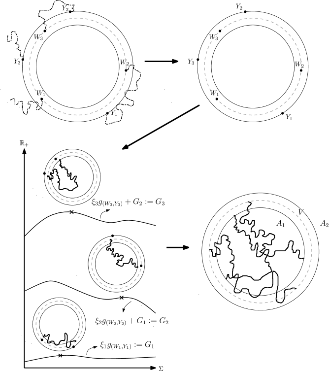
Figure 6: The figure shows how we will use the soft local times technique to simulate the range of a simple random walk trajectory intersected with $A_{1}$. We first simulate a process of pairs of points $((W_{k},Y_{k}),k\geq 0)$ denoting the entrance at $V$ and exit at $\partial A_{2}$ of a simple random walk trajectory that starts at $V$. We then use the soft local times method to simulate the pieces of trajectory that lie between each of the pairs $(W_{k},Y_{k})$.

It is clear from (2.2) the fact that in order to simulate the random interlacements set at level $u$ in a bounded subset $K$ of $\mathbb{Z}^{d}$ we need only to pick a $N^{u}_{K}\stackrel{{\scriptstyle\tiny d}}{{=}}\textit{Poisson}(u\operatorname{cap}(K))$ number of points in $\partial K$, each point chosen according to the measure $\overline{e}_{K}(\cdot)$, and from each point start a simple random walk.

We intend to study $\mathcal{I}^{u}_{A_{1}}=\mathcal{I}^{u}\cap A_{1}$, showing that this set is not much influenced by the random interlacements set intersected with $A_{2}$, $\mathcal{I}^{u}_{A_{2}}=\mathcal{I}^{u}\cap A_{2}$. We will later clarify what we mean by “influence”. For now, we observe that the only “information” $\mathcal{I}^{u}_{A_{1}}$ receives from $\mathcal{I}^{u}_{A_{2}}$ is the location of the entrance and exit points of the excursions on $\partial A_{2}$ of the random walks that constitute $\mathcal{I}^{u}_{A_{2}}$.

Let us begin the work towards our result. We first generate the points of entrance at $V$ and exit from $A_{2}^{C}$ of each excursion on $V$ of a random walk trajectory. These points will be the clothesline onto which we will hang the pieces of trajectory that meet $A_{1}$, we will do so using the soft local times method.

Let us define the successive return and departure times between $V$ and $A_{2}$. Given a trajectory that starts at $V$, we define

$$D_{0} =0,\qquad R_{1}=H_{\partial A_{2}},$$

(4.1) $$D_{1} =H_{V}\circ\theta_{R_{1}}+R_{1},\qquad R_{2}=H_{\partial A_{2}}\circ\theta_{D_{1}}+D_{1},$$

$$D_{2} =H_{V}\circ\theta_{R_{2}}+R_{2}\qquad$$ and so on.

We also define the random time

(4.2) $$T_{\Delta}=\inf\{k\geq 1;R_{k}=\infty\},$$

which is almost surely finite, as the walk is transient.

Let $(X_{n},n\geq 0)$ be the simple random walk with initial distribution given by $\overline{e}_{V}(\cdot)$. Let $\Delta$ be an artificial cemetery state. We construct a random sequence of elements of $(V\times\partial A_{2})\cup\{\Delta\}$ in the following way: Conditioned on the event $\{T_{\Delta}=m\}$, we let

$$\big{(}(W_{1},Y_{1}),\dots,(W_{m-1},Y_{m-1}),(W_{m},Y_{m}),(W_{m+1},Y_{m+1}),\dots\big{)}$$********************

$$=\big{(}(X_{D_{0}},X_{R_{1}}),\dots,(X_{D_{m-2}},X_{R_{m-1}}),\Delta,\Delta,\dots\big{)}.$$

It is then elementary to prove that the process $((W_{k},Y_{k}))_{k\geq 1}$ inherits the Markov property from the simple random walk. We call $((W_{k},Y_{k}))_{k\geq 1}$ the clothesline process started at $W_{1}$. When there is no risk of confusion we will also denote by $\mathbb{P}_{w_{0}}$ the probability measure associated with the clothesline process started at a given point $w_{0}\in V$.

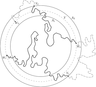
Figure 7: An example of the process $((W_{k},Y_{k}))_{k\geq 1}$.

Let us now use the soft local times method to generate the trajectories inside $A_{1}$, given the entrance and exit points $((W_{k},Y_{k}))_{k\geq 1}$. We first define the underlying space $\Sigma$ where our pieces of trajectories will live. We let $\mathcal{K}$ be the set of nearest-neighbor paths in $A_{2}^{C}$ with one endpoint in $\partial A_{1}$ and the other in $V$,

(4.3) $$\mathcal{K}:=\big{\{}(x_{0},x_{1},\dots,x_{n});n\in\mathbb{N},x_{i}\in A_{2}^{C}\text{ for $1\leq i\leq n$},x_{0}\in\partial A_{1},x_{n}\in V\big{\}}.$$

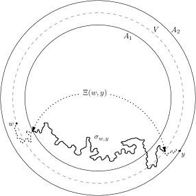
Figure 8: The definition of $\sigma(w,y)$ and $\Xi(w,y)$.

We introduce yet another artificial state $\Theta$ for reasons that will be made clear in a few moments. We let $\Sigma:=\mathcal{K}\cup\{\Theta\}$ and let $\mu$ be a measure on $\Sigma$ defined in the following way: given $A\subseteq\Sigma$,

(4.4) $$\mu(A):=\sum_{(x_{0},\dots,x_{n})\in A}\mathbb{P}_{(x_{0},x_{n})}[X_{0}=x_{0},\dots,X_{n}=x_{n}]+1_{\{\Theta\in A\}},$$

where $\mathbb{P}_{(x_{0},x_{n})}$ is the simple random walk measure conditioned on the event where $x_{0}$ is the walk’s initial point and $x_{n}$ is its last point on $V$ before reaching $\partial A_{2}$. Notice that $\mu(\{\Theta\})=1$.

Given $(w,y)\in V\times\partial A_{2}$ we let $\mathbb{P}_{w,y}$ be the measure associated with simple random walk starting at $w$ conditioned on the event where $y$ is the first point the walk hits in $\partial A_{2}$, that is:

(4.5) $$\mathbb{P}_{w,y}[\cdot]:=\mathbb{P}_{w}[\text{ }\cdot\mid X_{H_{\partial A_{2}}}=y]$$

We want to randomly select (according to the conditional simple random walk measure above) a piece of trajectory in $A_{1}$ given a starting point in $V$ and an ending point in $\partial A_{2}$. Given $w\in V$ and $y\in\partial A_{2}$ we define the random element $\sigma_{w,y}\in\Sigma$ in the following way:

• Let $\mathcal{B}_{w,y}$ be a Bernoulli random variable with parameter $\mathbb{P}_{w,y}[H_{\partial A_{1}}<H_{\partial A_{2}}]$.

• If $\mathcal{B}_{w,y}=0$ we let $\sigma_{w,y}\equiv\Theta$.

• If $\mathcal{B}_{w,y}=1$ we let, for $\mathfrak{A}\subseteq\mathcal{K}$:

  (4.6) $$\mathbb{P}[\sigma_{w,y}\in\mathfrak{A}]=\sum_{(a_{0},\dots,a_{n})\in\mathfrak{A}}\mathbb{P}_{w,y}\left[\begin{array}[]{c}X_{H_{A_{1}}}=a_{0},X_{H_{A_{1}}+1}=a_{1},\dots,X_{H_{A_{1}}+n}=a_{n},\\ X_{k}\notin A_{1}\text{ for every }k=H_{A_{1}}+n+1,\dots,H_{A_{2}}\end{array}\right].$$

In other words, the random element $\sigma_{w,y}\in\Sigma$ will either be $\Theta$, on the event where a random walk starting at $w$ and exiting at $y$ fails to reach $A_{1}$, or a simple random walk trajectory $(x_{0}^{w,y},x_{1}^{w,y},\dots,x_{k(w,y)}^{w,y})\in\mathcal{K}$ distributed so that $x_{0}^{w,y}$ is the first point in $A_{1}$ after the start at $w$ and $x_{k(w,y)}^{w,y}$ is the last point in $V$ before reaching $y\in\partial A_{2}$. We then define $g_{(w,y)}:\Sigma\mapsto\mathbb{R}_{+}$ to be the $\mu$-density of $\sigma_{w,y}$. We refer to Figure 8.

Given $z=(x_{0},\dots,x_{n})\in\mathcal{K}$ we denote by $\Xi(z)$ the pair $(x_{0},x_{n})$, the path’s starting and ending points. We also let $\Xi(\Theta)=\Theta$ so that $\Xi(z)$ is defined for all $z\in\Sigma$. For $(w,y)\in V\times\partial A_{2}$ we define $\Xi(w,y)$ to be the random element $\Xi(\sigma_{w,y})$.

Let us calculate $g_{(w,y)}$ using the above notation. For $\mathfrak{A}\subseteq\Sigma$ we want to express the probability $\mathbb{P}[\sigma_{w,y}\in\mathfrak{A}]$ as a $\mu$-integral over $\mathfrak{A}$.

(4.7) $$\begin{array}[]{e}\mathbb{P}[\sigma_{w,y}\in\mathfrak{A}]&=&\sum_{a\in\mathfrak{A}}\mathbb{P}[\sigma_{w,y}=a]\\ \hfil&=&1_{\{\Theta\in\mathfrak{A}\}}\mathbb{P}_{w,y}[\Xi(w,y)=\Theta]\\ \hfil\\ \hfil&\hfil&+\sum_{\begin{subarray}{c}a\in\mathfrak{A}\\ a\neq\Theta\end{subarray}}\mathbb{P}_{w,y}[\Xi(w,y)=\Xi(a)]\mathbb{P}_{w,y}[a\mid\Xi(w,y)=\Xi(a)]\\ \hfil&=&1_{\{\Theta\in\mathfrak{A}\}}\mathbb{P}_{w,y}[\Xi(w,y)=\Theta]+\sum_{\begin{subarray}{c}a\in\mathfrak{A}\\ a\neq\Theta\end{subarray}}\mathbb{P}_{w,y}[\Xi(w,y)=\Xi(a)]\mathbb{P}_{\Xi(a)}[a]\\ \hfil&=&\sum_{a\in\mathfrak{A}}\mathbb{P}_{w,y}[\Xi(w,y)=\Xi(a)]\mu(a)\\ \hfil&=&\int_{\mathfrak{A}}\mathbb{P}_{w,y}[\Xi(w,y)=\Xi(z)]\mu(\mathrm{d}z),\end{array}$$

so that $g_{(w,y)}(z)=\mathbb{P}_{w,y}[\Xi(w,y)=\Xi(z)]$. Notice that the function $g_{(w,y)}(z)$ only depends on the pair $\Xi(z)$, the path’s initial and ending points.

Let $(L,\mathcal{D},\mathbb{Q})$ be the measure space of the Poisson point process on $\Sigma\times\mathbb{R}_{+}$ with intensity measure $\mu\otimes\mathrm{d}v$, where $\mathrm{d}v$ is the Lebesgue measure on $\mathbb{R}_{+}$. A weighted sum of functions $g_{(\cdot,\cdot)}$ indexed by clothesline processes $((W_{k},Y_{k}))_{k\geq 1}$ will be the soft local time used to simulate the pieces of trajectory we need. This way we will be able to simulate the intersection of a simple random walk trajectory with $A_{1}$. As we have seen in the random interlacements process’s definition, to simulate the interlacements set inside $V$ we need a number $N^{u}_{V}\stackrel{{\scriptstyle\tiny d}}{{=}}Poisson(u\operatorname{cap}(V))$ of independent random walks. We will need the same number of independent clothesline processes. For such task we will need a much bigger probability space, easily definable as a product between the Poisson point process space and an infinite product of independent simple random walk spaces starting on $V$. We call this bigger space the global probability space, and denote by $\mathcal{P}$ its probability measure, which we will call the ‘global probability’.

Given a clothesline process $((W_{k},Y_{k}))_{k\geq 1}$, we define the trajectory’s soft local time:

(4.8) $$G(z)=\sum_{k=1}^{T_{\Delta}}\xi_{k}g_{(W_{k},Y_{k})}(z).$$

We will also need to consider the soft local time up to a random time $T\leq T_{\Delta}$:

(4.9) $$G_{T}(z)=\sum_{k=1}^{T}\xi_{k}g_{(W_{k},Y_{k})}(z).$$

Analogously, we define for any deterministic time $n\geq 1$

(4.10) $$G_{n}(z)=\sum_{k=1}^{n}\xi_{k}g_{(W_{k},Y_{k})}(z).$$

We denote by $z_{k}$ the piece of trajectory randomly selected by the $k$-th soft local time, $G_{k}$.

As we have seen before, in order to simulate the random interlacements set at level $u$ in $A_{1}$, we actually need a

$$N^{u}_{V}\stackrel{{\scriptstyle\tiny d}}{{=}}\textit{Poisson}(u\operatorname{cap}(V))$$

number of random walk trajectories, each started at a point in $V$ distributed as $\overline{e}_{V}(\cdot)$. For $j=1,\dots,N^{u}_{V}$ we let $((W_{k}^{j},Y_{k}^{j}))_{k\geq 1}$ be a clothesline process started at $W_{1}^{j}$, so that $((W_{k}^{j},Y_{k}^{j}))_{k\geq 1}$ is independent from $((W_{k}^{i},Y_{k}^{i}))_{k\geq 1}$ for $i\neq j$, and so that $W_{1}^{j}$ is distributed as $\overline{e}_{V}(\cdot)$. Let $T_{\Delta}^{j}$ be the killing time associated with $((W_{k}^{j},Y_{k}^{j}))_{k\geq 1}$. We denote by

(4.11) $$G^{j}(z)=\sum_{k=1}^{T_{\Delta}^{j}}\xi_{k}^{j}g_{(W_{k}^{j},Y_{k}^{j})}(z)$$

the soft local time associated with the $j$-th clothesline process. It should be clear from Proposition 3.2 that we can simulate all the random elements $(\sigma_{W_{k}^{j},Y_{k}^{j}})_{j,k\geq 1}$ at the same time using only one realization of a Poisson point process in $\Sigma\times\mathbb{R}_{+}$. As the Corollary 3.3 shows, in order to control the values our random elements take we only need to control the function

(4.12) $$G^{\Sigma}_{u}(z)=\sum_{j=1}^{N^{u}_{V}}G^{j}(z),$$

the soft local time associated with the whole process. With such objective in mind we for now set our goals at estimating the soft local time’s moments. We first show an easier way to express the expectation of $G(z)$.

Proposition 4.1.

Using the same notation as above, we have

(4.13) $$\mathbb{E}(G(z))=\mathbb{E}\Big{(}\sum_{k=1}^{T_{\Delta}}1_{\{\Xi(X_{D_{k-1}},X_{R_{k}})=\Xi(z)\}}\Big{)}.$$

Proof.

In fact,

(4.14) $$\begin{array}[]{e}\mathbb{E}(G(z))&=&\mathbb{E}\Big{(}\sum_{k=1}^{T_{\Delta}}g_{(W_{k},Y_{k})}(z)\Big{)}=\mathbb{E}\Big{(}\sum_{k=1}^{T_{\Delta}}\mathbb{P}_{W_{k},Y_{k}}[\Xi(W_{k},Y_{k})=\Xi(z)]\Big{)}\\ \hfil&=&\mathbb{E}\Big{(}\sum_{k=1}^{T_{\Delta}}1_{\{\Xi(W_{k},Y_{k})=\Xi(z)\}}\Big{)}=\mathbb{E}\Big{(}\sum_{k=1}^{T_{\Delta}}1_{\{\Xi(X_{D_{k-1}},X_{R_{k}})=\Xi(z)\}}\Big{)}.\end{array}$$

∎

We have then that the expectation of $G(z)$, for $z\neq\Theta$, is the same as the expectation of how many times a random walk started at $W_{1}$ will do a excursion on $A_{2}^{C}$ with starting and ending points given by $\Xi(z)$.

It is clear that the same computation works for any starting distribution for $W_{1}$. Given $y\in\partial A_{2}$, we let $\beta_{y}(\cdot)$ be the hitting measure on $V$ of a simple random walk started at $y$. We are then able to take $\beta_{y}(\cdot)$ as the starting distribution of $W_{1}$. Let then $\mathcal{P}_{\beta_{y}}$ be the global process’s measure in which the clothesline process’s starting distribution is given by $\beta_{y}(\cdot)$, and let $\mathbb{E}_{\beta_{y}}$ be its associated expectation. We are then required to allow the clothesline process to start at the cemetery state $\Delta$, denoting the failure of the random walk trajectory started at $y$ to reach $V$. In an analogous definition, we let $\mathcal{P}_{w_{0}}$ be the global process’s measure with $w_{0}\in V$ as the clothesline process’s starting point, and let $\mathbb{E}_{w_{0}}$ be its associated expectation.

The next proposition, adapted from Theorem $4.8$ of [13], gives a bound on the second moment $\mathbb{E}(G(z))^{2}$.

Proposition 4.2.

For any $w_{0}\in V$,

(4.15) $$\mathbb{E}_{w_{0}}\big{(}G(z)\big{)}^{2}\leq 2\mathbb{E}_{w_{0}}\big{(}G(z)\big{)}\big{(}\sup_{w^{\prime}\in V}\mathbb{E}_{w^{\prime}}G(z)+\sup_{w,y}g_{(w,y)}(z)\big{)}.$$

Proof.

Recall that the second moment of a $\mathop{\mathrm{Exp}}(1)$ random variable equals $2$. For $z\in\Sigma$ and $n\geq 1$, we write

$$\mathbb{E}_{w_{0}}\big{(}G_{n}(z)\big{)}^{2} =\mathbb{E}_{w_{0}}\Big{(}\sum_{k=1}^{n}\xi_{k}g_{(W_{k},Y_{k})}(z)\Big{)}^{2}$$

$$=\mathbb{E}_{w_{0}}\Big{(}\sum_{k=1}^{n}\xi_{k}^{2}g_{(W_{k},Y_{k})}^{2}(z)\Big{)}+\mathbb{E}_{w_{0}}\Big{(}2\sum_{k<k^{\prime}\leq n}\xi_{k}\xi_{k^{\prime}}g_{(W_{k},Y_{k})}(z)g_{(W_{k^{\prime}},Y_{k^{\prime}})}(z)\Big{)}$$

$$\leq\sum_{k=1}^{n}\mathbb{E}\xi_{k}^{2}\sup_{w,y}g_{(w,y)}(z)\mathbb{E}_{w_{0}}g_{(W_{k},Y_{k})}(z)+2\sum_{k=1}^{n-1}\sum_{k^{\prime}=k+1}^{n}\mathbb{E}_{w_{0}}\big{(}g_{(W_{k},Y_{k})}(z)g_{(W_{k^{\prime}},Y_{k^{\prime}})}(z)\big{)}$$

$$\leq 2\sup_{w,y}g_{(w,y)}(z)\mathbb{E}_{w_{0}}G_{n}(z)+2\sum_{k=1}^{n-1}\sum_{k^{\prime}=k+1}^{n}\mathbb{E}_{w_{0}}\big{(}g_{(W_{k},Y_{k})}(z)\mathbb{E}_{w_{0}}(g_{(W_{k}^{\prime},Y_{k}^{\prime})}(z)\mid W_{k},Y_{k})\big{)}$$

$$\leq 2\sup_{w,y}g_{(w,y)}(z)\mathbb{E}_{w_{0}}G_{n}(z)+2\sum_{k=1}^{n-1}\mathbb{E}_{w_{0}}\Big{(}g_{(W_{k},Y_{k})}(z)\mathbb{E}_{\beta_{Y_{k}}}\Big{(}\sum_{m=1}^{n-k}g_{(W_{m},Y_{m})}(z)\Big{)}\Big{)}$$

$$\leq 2\sup_{w,y}g_{(w,y)}(z)\mathbb{E}_{w_{0}}G_{n}(z)+2\sup_{w^{\prime}}\mathbb{E}_{w^{\prime}}\Big{(}\sum_{m=1}^{n-k}g_{(W_{m},Y_{m})}(z)\Big{)}\mathbb{E}_{w_{0}}\Big{(}\sum_{k=1}^{n-1}g_{(W_{k},Y_{k})}(z)\Big{)}$$

$$\leq 2\mathbb{E}_{w_{0}}\big{(}G_{n}(z)\big{)}\big{(}\sup_{w^{\prime}}\mathbb{E}_{w^{\prime}}G_{n}(z)+\sup_{w,y}g_{(w,y)}(z)\big{)},$$

so that the result is proved for time $n$. Letting $n$ go to infinity, by the monotone convergence theorem we can prove the result for the stopping time $T_{\Delta}$. ∎

For this paper’s results, an estimate on the exponential moments of $G$ will be essential. The next proposition, again adapted from [13] (propositions 4.3 and 4.2 are proved in the context of Markov chains in the original paper), gives us such an estimate.

Proposition 4.3.

Given $\hat{z}\in\Sigma$ and measurable $\Gamma\subset\Sigma$, let

(4.16) $$\begin{split}\alpha&=\inf\Big{\{}\frac{g_{(w,y)}(z^{\prime})}{g_{(w,y)}({\hat{z}})};(w,y)\in V\times\partial A_{2},z^{\prime}\in\Gamma,\hat{z}\in\mathcal{K}\Big{\}},\\ N(\Gamma)&=\#\{k\leq T_{\Delta};z_{k}\in\Gamma\},\text{ and}\\ \ell&\geq\;\smash{\sup_{(w,y)\in V\times\partial A_{2}}}\;g_{(w,y)}(\hat{z}).\end{split}$$

Then, for any $v\geq 2$,

(4.17) $$\mathcal{P}[G({\hat{z}})\geq v\ell]\leq\mathcal{P}[G({\hat{z}})\geq\ell]\Big{(}\exp\big{\{}-\big{(}\tfrac{v}{2}-1\big{)}\big{\}}+\sup_{w^{\prime}}\mathcal{P}_{w^{\prime}}\big{[}\eta(\Gamma\times[0,\tfrac{1}{2}v\ell\alpha])\leq N(\Gamma)\big{]}\Big{)}$$

(note that $\eta(\Gamma\times[0,\tfrac{1}{2}v\ell\alpha])$ is a random variable with distribution $\textnormal{Poisson}\big{(}\tfrac{1}{2}v\ell\alpha\mu(\Gamma)\big{)}$).

The number $\alpha=\alpha(\Gamma)$ above gives us a regularity condition: whenever $\alpha$ is uniformly larger than some constant $c>0$, we have that the density function $g_{(w,y)}(\cdot)$ when restricted to the subset $\Gamma$ cannot vary too much.

We first explain the intuition behind the terms in the right-hand side of  $(\ref{e_boundexpslt})$. The first term in the product is explained by the fact that in order for $G(\hat{z})$ to get past $v\ell$, it must first overcome $\ell$. The first summand inside the parenthesis corresponds to the probability that the sum $G(\hat{z})$ overcomes $\ell$ at the same “time” it overcomes $v\ell 2^{-1}$, that is, a overshooting probability. The second summand corresponds to a large deviation estimate, and generally, as $v$ grows, $N(\Gamma)$ becomes much smaller than the expected value of $\eta(\Gamma\times[0,\tfrac{1}{2}v\ell\alpha])$.

Proof.

We define the stopping time (with respect to the filtration $\mathcal{F}_{n}=\sigma((W_{k},Y_{k}),\xi_{k},k\leq n))$

(4.18) $$T_{\ell}=\inf\{k\geq 1;G_{k}({\hat{z}})\geq\ell\}.$$

For $v\geq 2$, we have

$$\mathcal{P}[G({\hat{z}})\geq v\ell]$$*************************************************

(4.19) $$\leq\mathcal{P}\big{[}T_{\ell}<\infty,\;G_{T_{\ell}}({\hat{z}})\geq\tfrac{v}{2}\ell\big{]}+\mathcal{P}\big{[}T_{\ell}<\infty,\;G_{T_{\ell}}({\hat{z}})<\tfrac{v}{2}\ell,\;G({\hat{z}})-G_{T_{\ell}}({\hat{z}})>\tfrac{v}{2}\ell\big{]}$$

(note that $\mathcal{P}[G({\hat{z}})\geq\ell]=\mathcal{P}[T_{\ell}<\infty]$). We first estimate the first term in the right side of the above inequality. By the memoryless property of the exponential distribution, we have

$$\smash{\sum_{n\geq 1}}\mathbb{E} \Big{(}G_{n-1}({\hat{z}})<\ell,\mathcal{P}\big{[}\xi_{n}g_{(W_{n},Y_{n})}({\hat{z}})>\tfrac{v}{2}\ell-G_{n-1}({\hat{z}})\mid W_{n-1},Y_{n-1},G_{n-1}\big{]}\Big{)}$$

$$\leq\sum_{n\geq 1}\mathbb{E}\Big{(}G_{n-1}({\hat{z}})<\ell,\mathcal{P}[\xi_{1}g_{(W_{n},Y_{n})}({\hat{z}})>\ell-G_{n-1}]\,\mathcal{P}\big{[}\xi_{1}g_{(W_{n},Y_{n})}({\hat{z}})>\big{(}\tfrac{v}{2}-1\big{)}\ell\big{]}\Big{)}$$

(4.20) $$\leq\mathcal{P}[T_{\ell}<\infty]\sup_{(w^{\prime},y^{\prime})}\mathcal{P}\big{[}\xi_{1}g_{(w^{\prime},y^{\prime})}({\hat{z}})>\big{(}\tfrac{v}{2}-1\big{)}\ell\big{]}$$

$$\leq\mathcal{P}[T_{\ell}<\infty]\exp\big{\{}-\big{(}\tfrac{v}{2}-1\big{)}\big{\}}.$$

Now, to bound the second term in the right side of (4.19), we write

(4.21) $$\begin{split}\mathbb{E}&\big{(}T_{\ell}<\infty,\;G_{T_{\ell}}(\hat{z})<\tfrac{v}{2}\ell,\mathcal{P}[G({\hat{z}})-G_{T_{\ell}}({\hat{z}})>\tfrac{v}{2}\ell\mid G_{1},\dots,G_{T_{\ell}}]\big{)}\\ &\leq\mathcal{P}\big{[}T_{\ell}<\infty\big{]}\;\smash{\sup_{w^{\prime}}}\;\mathcal{P}_{w^{\prime}}[G({\hat{z}})>\tfrac{v}{2}\ell].\end{split}$$

Using that for any $z^{\prime}\in\Sigma$

(4.22) $$G(z^{\prime})=\sum_{k=1}^{T_{\Delta}}\xi_{k}g_{(W_{k},Y_{k})}(z^{\prime})\geq\sum_{k=1}^{T_{\Delta}}\alpha\xi_{k}g_{(W_{k},Y_{k})}({\hat{z}}){{1}}_{\Gamma}(z^{\prime})=\alpha G({\hat{z}}){{1}}_{\Gamma}(z^{\prime}).$$

we obtain, for all $z^{\prime}$,

(4.23) $$\begin{split}\mathcal{P}\big{[}G({\hat{z}})\geq\tfrac{v}{2}\ell\big{]}&\leq\mathcal{P}\Big{[}G(z^{\prime})\geq\frac{1}{2}v\ell\alpha,\text{ for every $z^{\prime}\in\Gamma$}\Big{]}\\ &\leq\mathcal{P}\big{[}\eta(\Gamma\times[0,\tfrac{1}{2}v\ell\alpha])\leq N(\Gamma)\big{]}.\end{split}$$

Collecting (4.19), (4), (4.21) and (4.23) we finish the proof of the result. ∎

5 Conditional decoupling

We begin this section gathering some facts needed for the proof of the main theorem of this paper. But first we give an overview of main argument presented in this section. We will simulate the random interlacements set intersected with $A_{1}$ in two ways. In the first way we will simulate $\mathcal{I}_{A_{1}}^{u}$ using $G^{\Sigma}_{u}$, that is, we will simulate $\mathcal{I}_{A_{1}}^{u}$ using the soft local times indexed by the clothesline processes. In the second way, we will construct a set made up from random walk trajectories in $A_{1}$ in a similar way to the construction of $\mathcal{I}^{u}_{A_{1}}$, the only difference will be that the soft local times used in this second construction will be indexed by a given nonrandom sequence $\hat{\zeta}$ of pairs of points belonging $V\times\partial A_{2}$. We will denote this second random set by $\mathcal{I}^{u}_{A_{1}\mid\hat{\zeta}}$, and we will show using the soft local times method that $\mathcal{I}^{u}_{A_{1}\mid\hat{\zeta}}$ and $\mathcal{I}^{u}_{A_{1}}$ are usually very similar to each other. We then prove a similar result when the pairs of points that constitute the nonrandom sequence all belong to the boundary of a set contained in $A_{2}$.

Throughout this section we will again only differentiate between $A_{1}^{\tiny\Circle}$ and $A_{1}^{\tiny\Square}$ when the need arises. We start by stating the following bound

(5.1) $$\sup_{\begin{subarray}{c}w^{\prime}\in V\\ y^{\prime}\in\partial A_{2}\end{subarray}}\mathbb{P}_{w^{\prime},y^{\prime}}\big{[}\Xi(w^{\prime},y^{\prime})=(w_{0},y_{0})\big{]}\leq cs^{-2(d-1)},$$

for which the proof is technical and we thus postpone it to subsection A.1 of the appendix.

Let $z\in\Sigma$ be such that $\Xi(z)=(w_{0},y_{0})$, and let $h:=\operatorname{dist}(w_{0},y_{0})$. We let $F(w_{0},y_{0})$ stand for $G(z)$, making explicit the dependence of the soft local time on the endvertices $\Xi(z)$. We define

(5.2) $$\pi(w_{0},y_{0}):=\mathbb{E}(F(w_{0},y_{0})).$$

We define $f_{A_{1}}(w_{0},y_{0})$ to be the probability that the simple random walk started at $w_{0}$ visits $y_{0}$ before hitting $A_{2}$. We will prove in the appendix (see Section A.1, propositions A.2 and A.3) the following bounds for these probabilities:

• Given $(w_{0},y_{0})\in A_{1}^{\tiny\Circle}\times V^{\tiny\Circle}$, there are constants $c_{1},c_{2}>0$ such that

  (5.3) $$c_{1}\frac{s^{2}}{h^{d}}\leq f_{A_{1}^{\tiny\Circle}}(w_{0},y_{0})\leq c_{2}\frac{s^{2}}{h^{d}}.$$

• Let $(w_{0},y_{0})\in A_{1}^{\tiny\Square}\times V^{\tiny\Square}$, and recall the definition of $\mathfrak{H}_{r+2s}$, the unsmoothed version of ${A_{2}^{\tiny\Square}}^{C}$. Let $\mathfrak{H}^{d-1}_{i}$; $i=1,\dots,2d$; denote the $(d-1)$-dimensional hyperfaces of $\mathfrak{H}_{r+2s}$, and let $l^{w_{0}}_{i}:=\min\{\operatorname{dist}(w_{0},\mathfrak{H}^{d-1}_{i}),h\}$, and $l^{y_{0}}_{i}:=\min\{\operatorname{dist}(y_{0},\mathfrak{H}^{d-1}_{i}),h\}$. Then there are constants $c_{1},c_{2}>0$ such that

  (5.4) $$c_{1}\frac{l^{w_{0}}_{1}\dots l^{w_{0}}_{2d}}{h^{2d}}\cdot\frac{1}{h^{d-2}}\cdot\frac{l^{y_{0}}_{1}\dots l^{y_{0}}_{2d}}{h^{2d}}\leq f_{A_{1}^{\tiny\Square}}(w_{0},y_{0})\leq c_{2}\frac{l^{w_{0}}_{1}\dots l^{w_{0}}_{2d}}{h^{2d}}\cdot\frac{1}{h^{d-2}}\cdot\frac{l^{y_{0}}_{1}\dots l^{y_{0}}_{2d}}{h^{2d}}.$$

The following lemma, whose proof we also postpone to the appendix (Section A.2), gives us an estimate on $\pi(w_{0},y_{0})$.

Lemma 5.1.

Using the notation defined above we have, for constants $c_{1},c_{2},c_{3},c_{4}>0$:

• $c_{1}\operatorname{cap}(V)^{-1}s^{-1}f_{A_{1}}(w_{0},y_{0})\leq\pi_{A_{1}}(w_{0},y_{0})\leq c_{2}\operatorname{cap}(V)^{-1}s^{-1}f_{A_{1}}(w_{0},y_{0})$,
  

• $\mathbb{E}(F(w_{0},y_{0})^{2})\leq c_{3}\operatorname{cap}(V)^{-1}s^{-2d+2}f_{A_{1}}(w_{0},y_{0})$.
  
  Moreover, since $\operatorname{dist}(w_{0},y_{0})\geq s$, we have
  

• $\sup_{w_{0},y_{0}}\pi(w_{0},y_{0})\leq c_{4}\operatorname{cap}(V)^{-1}s^{-(d-1)}$.

We now provide a large deviation bound for $F(w_{0},y_{0})$.

Lemma 5.2.

There are constants $c,c_{1},c_{2}>0$ such that for every $(w_{0},y_{0})\in V\times\partial A_{2}$, we have

(5.5) $$\mathcal{P}\big{[}F(w_{0},y_{0})>vcs^{-2(d-1)}\big{]}\leq c_{1}s^{2d-3}f_{A_{1}}(w_{0},y_{0})\operatorname{cap}(V)^{-1}e^{-c_{2}v}$$

for any $v\geq 2$ (we can also assume $c_{2}\leq 1$ without loss of generality).

Proof.

In the proof of this particular result it will be important for us to distinguish between the constants. We will use Proposition 4.3 for $F(w_{0},y_{0})$, with

$$\Gamma_{w_{0},y_{0}}:=\{(w_{0}^{\prime},y_{0}^{\prime})\in\partial A_{1}\times V;\max\{\|w_{0}^{\prime}-w_{0}\|,\|y_{0}^{\prime}-y_{0}\|\}\leq c_{4}s\},$$

with $0<c_{4}<1$ defined in Section A.3 of the appendix.

Using the same notation as in Proposition 4.3, we note that $(\ref{supprob2})$ implies

$$l\leq cs^{-2(d-1)}$$

and observe that $\mu(\Gamma_{w_{0},y_{0}})\geq c_{5}s^{2(d-1)}$ for some constant $c_{5}>0$. Also, as can be seen in Section A.3 of the appendix, we have

$$\alpha\geq c_{3}>0.$$

Chebyshev’s inequality and Lemma 5.1 then imply

(5.6) $$\mathcal{P}\big{[}T_{l}<\infty\big{]}\leq\mathcal{P}\big{[}F(w_{0},y_{0})>cs^{-2(d-1)}\big{]}\leq\frac{\pi(w_{0},y_{0})}{cs^{-2(d-1)}}\leq c_{1}s^{2d-3}f_{A_{1}}(w_{0},y_{0})\operatorname{cap}(V)^{-1}.$$

We denote by $N(\Gamma_{w_{0},y_{0}})$ the number of times the simple random walk trajectory associated with $F(w_{0},y_{0})$ makes an excursion of the form $z^{\prime}\in\Sigma$ on $A_{2}^{C}$ such that $\Xi(z^{\prime})=(w^{\prime},y^{\prime})\in\Gamma_{w_{0},y_{0}}$. We also let $\eta_{w_{0},y_{0}}$ stand for the number of points of the Poisson process associated with our soft local times that belong to $\Gamma_{w_{0},y_{0}}\times\big{[}0,\frac{1}{2}vcc_{3}s^{-2(d-1)}\big{]}$. We note that both definitions are consistent with Proposition 4.3 and write

$$\mathcal{P}\Big{[}\eta_{w_{0},y_{0}}\leq N(\Gamma_{w_{0},y_{0}})\Big{]}\leq\mathcal{P}\Big{[}\eta_{w_{0},y_{0}}\leq\frac{cc_{3}c_{5}v}{4}\Big{]}+\mathcal{P}\Big{[}N(\Gamma_{w_{0},y_{0}})\geq\frac{cc_{3}c_{5}v}{4}\Big{]}.$$

We claim that both terms in the right side of the above inequality are exponentially small in $v$. To see why this is true, observe that:

• $\eta_{w_{0},y_{0}}$ has Poisson distribution with parameter at least $\frac{cc_{3}c_{5}v}{2}$, and

• every time the simple random walk associated with $F(w_{0},y_{0})$ hits $\partial A_{2}$, with uniform positive probability the walk never reaches $\Gamma_{w_{0},y_{0}}$ again. This way $N(\Gamma_{w_{0},y_{0}})$ is dominated by a Geometric$(c_{6})$ random variable, for some constant $c_{6}<1$.

Together with $(\ref{e_timebound})$ and Proposition 4.3, this finishes the proof of the lemma. ∎

Let $\Psi_{w_{0},y_{0}}(\lambda)=\mathbb{E}(e^{\lambda F(w_{0},y_{0})})$ be the moment generating function of $F(w_{0},y_{0})$. We are going to use the bounds above to estimate $\Psi_{w_{0},y_{0}}$. It is elementary to obtain that $e^{t}-1\leq t+t^{2}$ for $t\in[0,1]$. With this observation in mind, we write for $0\leq\lambda\leq\frac{c_{2}s^{2(d-1)}}{2c}$, where $c$ and $c_{2}$ are the same as in the theorem above:

$$\Psi_{w_{0},y_{0}}(\lambda)-1=\phantom{******}$$

$$\phantom{****}=\mathbb{E}(e^{\lambda F(w_{0},y_{0})}-1){{1}}_{\lambda F(w_{0},y_{0})\leq 1}+\mathbb{E}(e^{\lambda F(w_{0},y_{0})}-1){{1}}_{\lambda F(w_{0},y_{0})>1}$$

$$\phantom{****}\leq\mathbb{E}(\lambda F(w_{0},y_{0})+\lambda^{2}F(w_{0},y_{0})^{2})+\mathbb{E}(e^{\lambda F(w_{0},y_{0})}-1){{1}}_{\lambda F(w_{0},y_{0})>1}$$

$$\phantom{****}\leq\lambda\pi(w_{0},y_{0})+c_{1}\lambda^{2}\operatorname{cap}(V)^{-1}s^{-2d+2}f_{A_{1}}(w_{0},y_{0})+\mathbb{E}(e^{\lambda F(w_{0},y_{0})}-1){{1}}_{\lambda F(w_{0},y_{0})>1}$$

$$\phantom{****}\leq\lambda\pi(w_{0},y_{0})+c^{\prime}\lambda^{2}\operatorname{cap}(V)^{-1}s^{-2d+2}f_{A_{1}}(w_{0},y_{0})+\lambda\int\limits_{\lambda^{-1}}^{\infty}e^{\lambda y}\mathcal{P}\big{[}F(w_{0},y_{0})>y\big{]}\mathrm{d}y$$

$$\phantom{****}\leq\lambda\pi(w_{0},y_{0})+f_{A_{1}}(w_{0},y_{0})\operatorname{cap}(V)^{-1}\Big{(}c^{\prime}\lambda^{2}s^{-2d+2}+\lambda c^{\prime}s^{2d-3}\int\limits_{\lambda^{-1}}^{\infty}\exp{\Big{(}\frac{-c_{2}s^{2(d-1)}y}{2c}\Big{)}}\mathrm{d}y\Big{)}$$

$$\phantom{****}\leq\lambda\pi(w_{0},y_{0})+f_{A_{1}}(w_{0},y_{0})\operatorname{cap}(V)^{-1}\Big{(}c^{\prime}\lambda^{2}s^{-2d+2}+c^{\prime}\lambda s^{-1}\exp{\Big{(}\frac{-c_{2}s^{2(d-1)}\lambda^{-1}}{2c}\Big{)}}\Big{)}$$

(5.7) $$\phantom{****}\leq\lambda\pi(w_{0},y_{0})+c^{\prime}\lambda^{2}\operatorname{cap}(V)^{-1}s^{-2d+2}f_{A_{1}}(w_{0},y_{0}),$$

where we used Lemma 5.1 and Lemma 5.2. Now since $e^{-t}-1\leq-t+t^{2}$ for all $t\geq 0$, we obtain for $\lambda\geq 0$

(5.8) $$\Psi_{w_{0},y_{0}}(-\lambda)-1\leq-\lambda\pi(w_{0},y_{0})+c\lambda^{2}\operatorname{cap}(V)^{-1}s^{-2d+2}f_{A_{1}}(w_{0},y_{0}),$$

(the large deviation bound of Lemma 5.2 is not necessary is this case).

Observe that if $(\chi_{k},k\geq 1)$ are i.i.d. random variables with common moment generating function $\Psi$ and $N$ is an independent Poisson random variable with parameter $\theta$, then

$$\mathbb{E}\exp\big{(}\lambda\sum\limits_{k=1}^{N}\chi_{k}\big{)}=e^{(\theta(\Psi(\lambda)-1))}.$$

We let $F_{k}(w_{0},y_{0})$ denote the expectation $\mathbb{E}(G^{k}(z))$ defined in $(\ref{e_sltdef1})$, when $z\in\Sigma$ is such that $\Xi(z)=(w_{0},y_{0})$. Using Lemma 5.1 and $(\ref{e_moment1})$, we have, for $N_{\hat{u}}^{V}\stackrel{{\scriptstyle\tiny d}}{{=}}Poisson(\hat{u}\operatorname{cap}(V))$ and any $\delta>0$

(5.9) $$\begin{array}[]{e}\lx@intercol\@ADDCLASS{ltx_eqn_lefteqn}$\displaystyle\mathcal{P}\big{[}G^{\Sigma}_{\hat{u}}(z)\geq(1+\delta)\hat{u}\operatorname{cap}(V)\pi(w_{0},y_{0})\big{]}=\phantom{********}$\mbox{}\hfil\lx@intercol\\ \hfil&\phantom{********}=&\mathcal{P}\Big{[}\sum_{k=1}^{N_{\hat{u}}^{V}}F_{k}(w_{0},y_{0})\geq(1+\delta)\hat{u}\operatorname{cap}(V)\pi(w_{0},y_{0})\Big{]}\\ \hfil\\ \hfil&\phantom{********}\leq&\frac{\mathbb{E}(\exp\big{(}\lambda\sum_{k=1}^{N_{\hat{u}}^{V}}F_{k}(w_{0},y_{0})\big{)})}{\exp\big{(}\lambda(1+\delta)\hat{u}\operatorname{cap}(V)\pi(w_{0},y_{0})\big{)}}\\ \hfil\\ \hfil&\phantom{********}\leq&\exp\big{(}-\lambda(1+\delta)\hat{u}\operatorname{cap}(V)\pi(w_{0},y_{0})+\hat{u}\operatorname{cap}(V)(\Psi_{w_{0},y_{0}}(\lambda)-1)\big{)}\\ \hfil\\ \hfil&\phantom{********}\leq&\exp\big{(}-(\lambda\delta\hat{u}\operatorname{cap}(V)\pi(w_{0},y_{0})-c^{\prime}\lambda^{2}\hat{u}s^{-2d+2}f_{A_{1}}(w_{0},y_{0}))\big{)}\\ \hfil\\ \hfil&\phantom{********}\leq&\exp\big{(}-(\lambda\delta\hat{u}cs^{-1}f_{A_{1}}(w_{0},y_{0})-c^{\prime}\lambda^{2}\hat{u}s^{-2d+2}f_{A_{1}}(w_{0},y_{0}))\big{)}.\end{array}$$

Analogously, with $(\ref{e_moment2})$ instead of $(\ref{e_moment1})$, we obtain

(5.10) $$\mathcal{P}\big{[}G^{\Sigma}_{\hat{u}}(z)\leq(1-\delta)\hat{u}\operatorname{cap}(V)\pi(w_{0},y_{0})\big{]}\leq\exp\big{(}-(\lambda\delta\hat{u}cs^{-1}-c^{\prime}\lambda^{2}\hat{u}s^{-2d+2})f_{A_{1}}(w_{0},y_{0})\big{)}.$$

We choose $\lambda=c_{7}\delta s^{2d-3}$ with $c_{7}$ small enough so that $\lambda\leq\frac{c_{2}s^{2(d-1)}}{2c}$, and observe that the bounds for $f_{A_{1}}(w_{0},y_{0})$ given in $(\ref{e_circlebound})$ and $(\ref{e_squarebound})$ imply

$$\inf_{w_{0},y_{0}}f_{A_{1}^{\tiny\Square}}(w_{0},y_{0}) \geq cs^{2d}r^{-3d+2},$$

$$\inf_{w_{0},y_{0}}f_{A_{1}^{\tiny\Circle}}(w_{0},y_{0}) \geq cs^{2}r^{-d}.$$

Recall the definition of $b_{A_{1}^{\tiny\Circle}}$, a number such that

$$1\leq b_{A_{1}^{\tiny\Circle}}<\frac{2d-2}{d},$$

and the definition of $b_{A_{1}^{\tiny\Square}}$, a number such that

$$1\leq b_{A_{1}^{\tiny\Square}}<\frac{4d-4}{3d-2}.$$

Recall that $r\asymp s^{b_{A_{1}}}$. Then there exist constants $a_{A_{1}^{\tiny\Circle}}=2d-2-db_{A_{1}^{\tiny\Circle}}>0$ and $a_{A_{1}^{\tiny\Square}}=4d-4-3db_{A_{1}^{\tiny\Square}}+2b_{A_{1}^{\tiny\Square}}>0$ such that

$$\mathcal{P}\big{[}G^{\Sigma}_{\hat{u}}(z)\geq(1+\delta)\hat{u}\operatorname{cap}(V)\pi(w_{0},y_{0})\big{]}\leq\exp\big{(}-c\delta^{2}\hat{u}s^{a_{A_{1}}}\big{)}.$$

Using the union bound (note that $\partial A_{1}\times V$ has $O(r^{2(d-1)})$ elements),

$$\mathcal{P}\big{[}(1-\delta)\hat{u}\operatorname{cap}(V)\pi(\Xi(z))\leq G^{\Sigma}_{\hat{u}}(z)\leq(1+\delta)\hat{u}\operatorname{cap}(V)\pi(\Xi(z))\text{, for all $z\in\mathcal{K}$}\big{]}\geq$$

(5.11) $$\geq 1-cr^{2(d-1)}\exp\big{(}-c^{\prime}\delta^{2}\hat{u}s^{a_{A_{1}}}\big{)}.$$

Observe that we can suppose $c^{\prime}\leq 1$ without loss of generality. We define the interval

$$I_{\hat{u},z}^{\delta}:=[(1-\delta)\hat{u}\operatorname{cap}(V)\pi(\Xi(z)),(1+\delta)\hat{u}\operatorname{cap}(V)\pi(\Xi(z))]$$

and the event

$$D_{\hat{u}}^{\delta}:=\{G_{\hat{u}}^{\Sigma}\in I_{\hat{u},z}^{\delta}\text{ for all $z\in\mathcal{K}$}\}.$$

Using $(\ref{e_moment5})$ and the union bound we obtain, for $\varepsilon>0$ sufficiently small,

$$\mathcal{P}\Big{[}D_{u}^{\varepsilon/4},D_{u(1-\varepsilon)}^{\varepsilon/4},D_{u(1+\varepsilon)}^{\varepsilon/4}\Big{]}\geq 1-cr^{2(d-1)}\exp\big{(}-c^{\prime}\varepsilon^{2}us^{a}\big{)}.$$

Since $r\asymp s^{b_{A_{1}}}$, by replacing the constants $c$ and $c^{\prime}$ in the above equation we obtain

(5.12) $$\mathcal{P}\Big{[}D_{u}^{\varepsilon/4},D_{u(1-\varepsilon)}^{\varepsilon/4},D_{u(1+\varepsilon)}^{\varepsilon/4}\Big{]}\geq 1-c\exp\big{(}-c^{\prime}\varepsilon^{2}us^{a}\big{)}.$$

We have just proved that with high probability, the soft local time associated to each of the processes $\mathcal{I}^{u}_{A_{1}}$, $\mathcal{I}^{u(1-\varepsilon)}_{A_{1}}$ and $\mathcal{I}^{u(1+\varepsilon)}_{A_{1}}$ stays confined between the graphs of two explicit deterministic functions. This happened when we let the “information” given by $\mathcal{I}^{u}_{A_{2}}$; namely the points of entrance at $V$ and exit at $\partial A_{2}$ of the excursions on $A_{1}$ of the simple random walk trajectories of the interlacements process at level $u$; to be distributed according to the right law, that is, the law of the clothesline processes. When we “average” those points according to these laws we obtain a good concentration for the whole function $G_{u}^{\Sigma}$, but our goal is to obtain a similar concentration when these points are deterministic. The heuristic argument is that when something happens with high probability in the annealed law, then most of the times it will also happen with high probability in the quenched law. We will introduce some new notation to make this argument rigorous and prove our main theorem.

Given any two finite sets $K_{1},K_{2}\subset\mathbb{Z}^{d}$, not necessarily disjoint, we want to describe a collection of generalized clothesline processes between $K_{1}$ and $K_{2}$ associated with the interlacements process at level $u$. We construct an infinite family $(X^{(j)}_{k},k\geq 0)_{0<j<\infty}$ of independent simple random walks with starting point distributed according to the normalized harmonic measure on $K_{1}$, as we did in definition (2.2). We let $\tau^{j}_{0}\equiv 0$ and define inductively

$$\begin{array}[]{e}\tau_{k+1}^{j}&:=1\{X^{(j)}_{\tau_{k}^{j}}\in K_{1}\}\inf\{t>\tau_{k+1}^{j};X^{(j)}_{t}\in K_{2}\}\\ \hfil&\qquad+1\{X^{(j)}_{\tau_{k}^{j}}\in K_{2}\}\inf\{t>\tau_{k+1}^{j};X^{(j)}_{t}\in K_{1}\},\end{array}$$

where $1\{\cdot\}$ denotes the indicator function of an event. We also define the random time

$$T_{j}:=\inf_{k\geq 0}\{\tau_{k+1}^{j}=\infty\}.$$

We let yet again $N_{u}^{K_{1}}\stackrel{{\scriptstyle\tiny d}}{{=}}\textit{Poisson}(u\operatorname{cap}(K_{1}))$ be a random variable independent from

$$(X^{(j)}_{k},k\geq 0)_{0<j<\infty}.$$

We then define the interlacements’ clothesline processes between $K_{1}$ and $K_{2}$ at level $u$ by

$$\mathrm{Cloth}_{u}(K_{1},K_{2}):=\Big{\{}\big{(}X^{(j)}_{\tau^{j}_{k}}\big{)}_{k=0}^{T_{j}}\Big{\}}_{j=1}^{N_{u}^{K_{1}}}.$$

When $K_{1}=V$ and $K_{2}=\partial A_{2}$, we have

$$\mathrm{Cloth}_{u}(V,\partial A_{2})\stackrel{{\scriptstyle\tiny d}}{{=}}\Big{\{}\big{(}W^{j}_{k},Y^{j}_{k}\big{)}_{k=1}^{T^{j}_{\Delta}}\Big{\}}_{j=1}^{N_{u}^{V}}.$$

We define

$$\Big{(}\mathcal{S}_{u}(K_{1},K_{2}),\sigma_{u}(K_{1},K_{2}),\mathbb{P}^{u}_{K_{1},K_{2}}\Big{)}$$

to be the probability space in which $\mathrm{Cloth}_{u}(K_{1},K_{2})$ is defined, and in which $\sigma_{u}(K_{1},K_{2})$ is the smallest $\sigma$-field in which $\mathrm{Cloth}_{u}(K_{1},K_{2})$ is measurable. If $\hat{\zeta}\in\mathcal{S}_{u}(V,\partial A_{2})$ and $\mathbb{P}^{u}_{V,\partial A_{2}}(\hat{\zeta})>0$, then we can write $\hat{\zeta}$ as a finite collection of finite sequences of points belonging to $V$ and $\partial A_{2}$

$$\hat{\zeta}:=\big{\{}\hat{\zeta}_{1},\dots,\hat{\zeta}_{K}\big{\}},$$

where for each $j=1,\dots,K$; $\hat{\zeta}_{j}$ is a finite sequence alternating between points of $V$ and $\partial A_{2}$. In other words, $\hat{\zeta}_{j}$ is a possible realization of a clothesline process. We write

$$\hat{\zeta}_{j}:=\big{(}\zeta^{j}_{0},\dots,\zeta^{j}_{n(j)}\big{)},$$

where $n(j)$ is odd, every even entry belongs to $V$ and every odd entry belongs to $\partial A_{2}$.

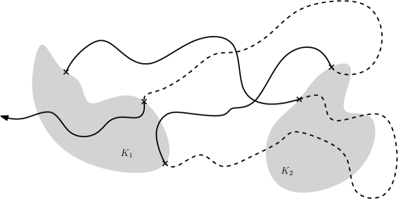
Figure 9: The generalized clothesline process between $K_{1}$ and $K_{2}$, here represented by the X marks.

We then define the soft local time associated with $\hat{\zeta}$. Using the same realization of the Poisson point process on $\Sigma\times\mathbb{R}_{+}$ defined on Section 4, we construct the soft local times

$$G^{\hat{\zeta}_{j}}(z):=\sum_{k=0}^{\frac{n(j)+1}{2}}\tilde{\xi}_{k}^{j}g_{(\zeta^{j}_{2k},\zeta_{2k_{1}}^{j})}(z),$$

where $\tilde{\xi}^{j}_{k}$ is an exponential random variable defined in the manner of (4.8). We then define

$$G^{\hat{\zeta}}(z):=\sum_{j=1}^{K}G^{\hat{\zeta}_{j}}(z).$$

This function should be viewed as a quenched version of the soft local times $G^{\Sigma}_{u}$, when the collection o clothesline processes $\{(W^{j}_{k},Y^{j}_{k})_{k=1}^{T^{j}_{\Delta}}\}_{j=1}^{N_{u}^{V}}$ is given by yhe deterministic element $\hat{\zeta}$. We denote by $\mathcal{I}^{u}_{A_{1}\mid\hat{\zeta}}$ the interlacements process inside $A_{1}$ determined by the ranges of the excursions of $\Sigma$ bellow $G^{\hat{\zeta}}$. $\mathcal{I}^{u}_{A_{1}\mid\hat{\zeta}}$ is distributed as the random interlacements process inside $A_{1}$ when its associated random walks excursions have entrance points at $V$ and exit points at $\partial A_{2}$ given by $\hat{\zeta}$. The next proposition implies that $G^{\hat{\zeta}}$ is usually between $G^{\Sigma}_{u(1-\varepsilon)}$ and $G^{\Sigma}_{u(1+\varepsilon)}$ with high probability.

Proposition 5.3.

There exists a set $\mathcal{A}\in\sigma_{u}(V,\partial A_{2})$ such that

$$\mathbb{P}^{u}_{V,\partial A_{2}}\big{[}\mathcal{A}\big{]}\geq 1-\exp\Big{(}-\frac{c^{\prime}}{2}\varepsilon^{2}us^{a_{A_{1}}}\Big{)},$$

and for all fixed $\hat{\zeta}\in\mathcal{A}$,

$$\mathcal{P}\big{[}G_{u(1-\varepsilon)}^{\Sigma}(z)\leq G^{\hat{\zeta}}(z)\leq G_{u(1+\varepsilon)}^{\Sigma}(z)\text{ for all $z\in\mathcal{K}$}\big{]}$$*********************

$$\phantom{*****}\geq 1-c\exp\Big{(}-\frac{c^{\prime}}{2}\varepsilon^{2}us^{a_{A_{1}}}\Big{)}.$$

Proof.

Observe that $(\ref{e_moment6})$ implies

$$\int\mathcal{P}\big{[}G_{u(1-\varepsilon)}^{\Sigma}(z)\leq G^{\hat{\zeta}}(z)\leq G_{u(1+\varepsilon)}^{\Sigma}(z)\text{ for all $z\in\mathcal{K}$}\big{]}\mathbb{P}^{u}_{V,\partial A_{2}}\big{[}\mathrm{d}\hat{\zeta}\big{]}$$************************

(5.13) $$\phantom{********}\geq 1-c\exp\big{(}-c^{\prime}\varepsilon^{2}us^{a_{A_{1}}}\big{)}.$$

Let

$$\begin{array}[]{e}\lx@intercol\@ADDCLASS{ltx_eqn_lefteqn}$\displaystyle\mathcal{A}:=\Big{\{}\hat{\zeta}\in\mathcal{S}_{u}(V,\partial A_{2})\text{ such that: }\mathcal{P}\big{[}G_{u(1-\varepsilon)}^{\Sigma}(z)\leq G^{\hat{\zeta}}(z)\leq G_{u(1+\varepsilon)}^{\Sigma}(z)\text{ for all $z\in\mathcal{K}$}\big{]}$\mbox{}\hfil\lx@intercol\phantom{********************}\\ \hfil&\phantom{*************}\geq 1-c\exp\Big{(}-\frac{c^{\prime}}{2}\varepsilon^{2}us^{a_{A_{1}}}\Big{)}\Big{\}}.\end{array}$$

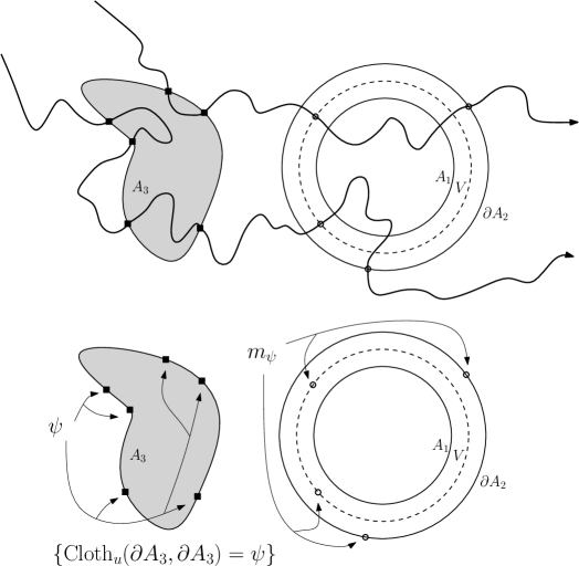
Figure 10: A visual representation of the random element $m_{\hat{\psi}}$.

Then $(\ref{e_moment7})$ implies

$$\mathbb{P}^{u}_{V,\partial A_{2}}\big{[}\mathcal{A}\big{]}+\Big{(}1-c\exp\Big{(}-\frac{c^{\prime}}{2}\varepsilon^{2}us^{a_{A_{1}}}\Big{)}\Big{)}\Big{(}1-\mathbb{P}^{u}_{V,\partial A_{2}}\big{[}\mathcal{A}\big{]}\Big{)}$$*****************************

$$\geq 1-c\exp\big{(}-c^{\prime}\varepsilon^{2}us^{a_{A_{1}}}\big{)},$$

so that

$$\mathbb{P}^{u}_{V,\partial A_{2}}\big{[}\mathcal{A}\big{]}\geq 1-\exp\Big{(}-\frac{c^{\prime}}{2}\varepsilon^{2}us^{a_{A_{1}}}\Big{)}.$$

This finishes the proof of the proposition. ∎

Figure 11: When the sequence $\hat{\zeta}$ belongs to a well behaved set $\mathcal{A}$, the decoupling probability is greater than $1-c\exp\Big{(}-\frac{c^{\prime}}{2}\varepsilon^{2}us^{a_{A_{1}}}\Big{)}$. The symbol $\varphi$ in the figure stands for the function $u\operatorname{cap}(V)\pi(\Xi(z))$. The figure shows the decoupling event, where $G_{u(1-\varepsilon)}^{\Sigma}(z)\leq G^{\hat{\zeta}}(z)\leq G_{u(1+\varepsilon)}^{\Sigma}(z)$ for all $z\in\mathcal{K}$.

Proposition 5.3 implies that, for $\hat{\zeta}\in\mathcal{A}$, there exists a process ($\hat{\mathcal{I}}^{u}_{A_{1}}$, $u\geq 0$) distributed as the random interlacements set intersected with $A_{1}$, and a coupling $\mathcal{P}$ such that, for all $\varepsilon>0$ sufficiently small and $r>0$ sufficiently big, we have

(5.14) $$\mathcal{P}\big{[}\hat{\mathcal{I}}^{u(1-\varepsilon)}_{A_{1}}\subseteq\mathcal{I}^{u}_{A_{1}\mid\hat{\zeta}}\subseteq\hat{\mathcal{I}}^{u(1+\varepsilon)}_{A_{1}}\big{]}\geq 1-c\exp\Big{(}-\frac{c^{\prime}}{2}\varepsilon^{2}us^{a_{A_{1}}}\Big{)}.$$

To complete the proof of our main theorem we need to show that a result similar to Proposition 5.3 remains valid under a different conditioning.

Let $A_{3}\subset A_{2}$ be such that $|\partial A_{3}|<\infty$, and write $\mathcal{I}^{u}_{A_{3}}:=\mathcal{I}^{u}\cap A_{3}$ . Then $\mathrm{Cloth}_{u}(\partial A_{3},\partial A_{3})$ is well defined. Given $\hat{\psi}\in\mathcal{S}_{u}(\partial A_{3},\partial A_{3})$, we define $m_{\hat{\psi}}\equiv m_{\hat{\psi}}(\partial A_{3})$ as a random element of $\mathcal{S}_{u}(V,\partial A_{2})$ distributed as $\mathrm{Cloth}_{u}(V,\partial A_{2})$ conditioned on the event where the entrance and exit points at $\partial A_{3}$ of the simple random walk excursions of $\mathcal{I}^{u}_{A_{3}}$ are given by $\hat{\psi}$. We denote by $\mathcal{I}^{u}_{A_{1}\mid\hat{\psi}}$ the random interlacements process on $A_{1}$ conditioned on the event where $\mathrm{Cloth}_{u}(\partial A_{3},\partial A_{3})$ is equal to the deterministic element $\hat{\psi}$. Notice that all “information” given by $\mathcal{I}^{u}_{A_{3}}$ to $\mathcal{I}^{u}\cap A_{3}^{C}$ is contained in $\mathrm{Cloth}_{u}(\partial A_{3},\partial A_{3})$, that is, conditioned on $\mathrm{Cloth}_{u}(\partial A_{3},\partial A_{3})$, $\mathcal{I}^{u}_{A_{3}}$ and $\mathcal{I}^{u}\cap A_{3}^{C}$ are independent.

Inequality (5.14) then implies, for $\hat{\psi}\in\mathcal{S}_{u}(\partial A_{3},\partial A_{3})$,

$$\mathcal{P}\big{[}\hat{\mathcal{I}}^{u(1-\varepsilon)}_{A_{1}}\subseteq\mathcal{I}^{u}_{A_{1}\mid\hat{\psi}}\subseteq\hat{\mathcal{I}}^{u(1+\varepsilon)}_{A_{1}}\big{]} =\!\!\!\!\!\!\!\!\!\sum_{\hat{\zeta}\in\mathcal{S}_{u}(V,\partial A_{2})}\!\!\!\!\mathcal{P}\big{[}\hat{\mathcal{I}}^{u(1-\varepsilon)}_{A_{1}}\subseteq\mathcal{I}^{u}_{A_{1}\mid\hat{\psi}}\subseteq\hat{\mathcal{I}}^{u(1+\varepsilon)}_{A_{1}}\mid m_{\hat{\psi}}=\hat{\zeta}\big{]}\mathcal{P}\big{[}m_{\hat{\psi}}=\hat{\zeta}\big{]}$$

$$=\!\!\!\!\!\!\!\!\!\sum_{\hat{\zeta}\in\mathcal{S}_{u}(V,\partial A_{2})}\!\!\!\!\mathcal{P}\big{[}\hat{\mathcal{I}}^{u(1-\varepsilon)}_{A_{1}}\subseteq\mathcal{I}^{u}_{A_{1}\mid\hat{\zeta}}\subseteq\hat{\mathcal{I}}^{u(1+\varepsilon)}_{A_{1}}\big{]}\mathcal{P}\big{[}m_{\hat{\psi}}=\hat{\zeta}\big{]}$$

(5.15) $$\geq\Big{(}1-c\exp\Big{(}-\frac{c^{\prime}}{2}\varepsilon^{2}us^{a_{A_{1}}}\Big{)}\Big{)}\mathcal{P}\big{[}m_{\hat{\psi}}\in\mathcal{A}\big{]}.$$

Let $\mathcal{E}$ be the set of all $\hat{\psi}\in\mathcal{S}_{u}(\partial A_{3},\partial A_{3})$ such that

$$\mathcal{P}\big{[}m_{\hat{\psi}}\in\mathcal{A}^{C}\big{]}\geq\sqrt{\mathbb{P}^{u}_{V,\partial A_{2}}\big{[}\mathcal{A}^{C}\big{]}}.$$

Since

$$\mathbb{P}^{u}_{V,\partial A_{2}}\big{[}\mathcal{A}^{C}\big{]}=\int\mathcal{P}\big{[}m_{\hat{\psi}}\in\mathcal{A}^{C}\big{]}\mathbb{P}^{u}_{\partial A_{3},\partial A_{3}}\big{[}\mathrm{d}\hat{\psi}\big{]}\geq\mathbb{P}^{u}_{\partial A_{3},\partial A_{3}}\big{[}\mathcal{E}\big{]}\sqrt{\mathbb{P}^{u}_{V,\partial A_{2}}\big{[}\mathcal{A}^{C}\big{]}},$$

we have

$$\mathbb{P}^{u}_{\partial A_{3},\partial A_{3}}\big{[}\mathcal{E}\big{]}\leq\sqrt{\mathbb{P}^{u}_{V,\partial A_{2}}\big{[}\mathcal{A}^{C}\big{]}}.$$

We have proved the following theorem, which implies Theorem 2.1:

Theorem 5.4.

Using the same notation as above, we have that, for constants $c,c^{\prime}>0$, there exists a set $\mathcal{G}\in\sigma_{u}(\partial A_{3},\partial A_{3})$ such that

$$\mathbb{P}^{u}_{\partial A_{3},\partial A_{3}}\big{[}\mathcal{G}\big{]}\geq 1-\exp\Big{(}-\frac{c^{\prime}}{4}\varepsilon^{2}us^{a_{A_{1}}}\Big{)},$$

and for all $\hat{\psi}\in\mathcal{G}$,

(5.16) $$\mathcal{P}\big{[}\hat{\mathcal{I}}^{u(1-\varepsilon)}_{A_{1}}\subseteq\mathcal{I}^{u}_{A_{1}\mid\hat{\psi}}\subseteq\hat{\mathcal{I}}^{u(1+\varepsilon)}_{A_{1}}\big{]}\geq 1-c\exp\Big{(}-\frac{c^{\prime}}{2}\varepsilon^{2}us^{a_{A_{1}}}\Big{)}.$$

Moreover, for any increasing function $f$ on the interlacements set intersected with $A_{1}$, with $\sup|f|<M$, we have

$$\big{(}\mathbb{E}(f(\mathcal{I}^{u(1-\varepsilon)}_{A_{1}}))-cM\exp\big{(}-c^{\prime}\varepsilon^{2}us^{a_{A_{1}}}\big{)}\big{)}{{1}}_{\mathcal{G}}\leq\mathbb{E}(f(\mathcal{I}^{u}_{A_{1}})\mid\mathcal{I}^{u}_{A_{3}}){{1}}_{\mathcal{G}}$$

(5.17) $$\leq\big{(}\mathbb{E}(f(\mathcal{I}^{u(1+\varepsilon)}_{A_{1}}))+cM\exp\big{(}-c^{\prime}\varepsilon^{2}us^{a_{A_{1}}}\big{)}\big{)}{{1}}_{\mathcal{G}}.$$

We finish the section with a brief proof of Theorem 2.2.

Proof of Theorem 2.2.

Note that, on equation (5.9), $\delta$ can be any real number greater than $0$, whereas in equation (5.10), we need to have $0<\delta<1$. Recall that $u^{\prime}>u>0$. We have, by substituting the appropriate $\delta$ in $\eqref{e_moment5}$ and ignoring the union bound term $cr^{2d-2}$,

$$\mathcal{P}\big{[}G^{\Sigma}_{u}(z)<G^{\Sigma}_{u+u^{\prime}}(z)\big{]} \geq 1-\mathcal{P}\big{[}G^{\Sigma}_{u}(z)>(u+u^{\prime}4^{-1})\operatorname{cap}(V)\pi(\Xi(z))\big{]}$$

$$\quad-\mathcal{P}\big{[}G^{\Sigma}_{u+u^{\prime}}(z)<2^{-1}(u+u^{\prime})\operatorname{cap}(V)\pi(\Xi(z))\big{]}$$

$$\geq 1-\exp\left(-\textasciidieresis\frac{c}{4}(u+u^{\prime})s^{a_{A_{1}}}\right)-\exp\left(-\frac{c}{16}\frac{(u^{\prime})^{2}}{u^{2}}us^{a_{A_{1}}}\right)$$

$$\geq 1-\exp\left(-c^{\prime}u^{\prime}s^{a_{A_{1}}}\right).$$

Now, proceeding in the same manner as we did in the proof of Theorem 5.4, we are able to prove Theorem 2.2. ∎

Appendix A Technical estimates

A.1 Bounding the relevant probabilities

For $w_{0}\in\partial A_{1}$ and $y_{0}\in V$ we want to bound the supremum

(A.1) $$\sup_{\begin{subarray}{c}w^{\prime}\in V\\ y^{\prime}\in\partial A_{2}\end{subarray}}\mathbb{P}_{w^{\prime},y^{\prime}}\big{[}\Xi(w^{\prime},y^{\prime})=(w_{0},y_{0})\big{]}$$

from above. To do so we will bound the “hanging” probability $\mathbb{P}_{w,y}\big{[}\Xi(w,y)=(w_{0},y_{0})\big{]}$ for arbitrary $w\in V$ and $y\in\partial A_{2}$.

Given a finite nearest neighbor path $\gamma$, we denote by $|\gamma|$ its length. We will say that a path $\gamma$ belongs to an event $E$ if $E$ occurs every time the simple random walk $(X_{k},k\geq 0)$ first $|\gamma|$ steps coincide with $\gamma$. We also let $\mathbb{P}_{x}\big{[}\gamma\big{]}$ denote the probability that the first $|\gamma|$ steps of the simple random walk started at $x$ coincide with $\gamma$.

In order to avoid a cumbersome notation we now introduce what, hopefully, will be a simpler way to denote our events of interest. For $w,y_{0}\in V$, $w_{0}\in\partial A_{1}$ and $y\in\partial A_{2}$ we define:

• $w\xrightarrow{1}w_{0}$: The collection of all finite nearest-neighbor trajectories starting at $w$ that do not reach neither $\partial A_{1}$ nor $\partial A_{2}$, except at its ending point $w_{0}\in\partial A_{1}$. Note that this collection can be thought of as the event where the simple random walk started at $w$ hits $\partial A_{1}$ for the first time at $w_{0}$ before reaching $\partial A_{2}$.
  

• $w_{0}\xrightarrow{2}y_{0}$: The collection of all finite nearest-neighbor trajectories starting at $w_{0}$ and ending at $y_{0}$ without reaching $\partial A_{2}$.
  

• $y_{0}\xrightarrow{3}y$: The collection of all finite nearest-neighbor trajectories starting at $y_{0}$ that hit $\partial A_{2}$ for the first time at $y$ before returning to $V$. Note that this collection can be thought of as the event where the simple random walk started at $y_{0}$ hits $\partial A_{2}$ before returning to $V$ and its entrance point in $\partial A_{2}$ is $y$.
  

• $w\xrightarrow{4}y$: The event where the entrance point in $\partial A_{2}$ of the simple random walk started at $w$ is $y$. This event clearly can also be regarded as a collection of simple random walk trajectories starting at $w$ and hitting $\partial A_{2}$ for the first time at $y$.

Figure 12: $\gamma$ as the concatenation of the three paths $\gamma_{1}$, $\gamma_{2}$ and $\gamma_{3}$.

We also let $w\xrightarrow{1}w_{0}\xrightarrow{2}y_{0}\xrightarrow{3}y$ be the “concatenation” of the first three collections, where the first trajectory’s ending point becomes the second trajectory’s starting point and so on. That is, if $\gamma\in w\xrightarrow{1}w_{0}\xrightarrow{2}y_{0}\xrightarrow{3}y$ then $\gamma$ is the concatenation of three distinct paths: $\gamma_{1}\in w\xrightarrow{1}w_{0}$, $\gamma_{2}\in w_{0}\xrightarrow{2}y_{0}$, $\gamma_{3}\in y_{0}\xrightarrow{3}y$. Note that, as an event,

$$w\xrightarrow{1}w_{0}\xrightarrow{2}y_{0}\xrightarrow{3}y=\{\Xi(w^{\prime},y^{\prime})=(w_{0},y_{0})\}.$$

With our new notation the hanging probability becomes

(A.2) $$\mathbb{P}_{w}\big{[}w\xrightarrow{1}w_{0}\xrightarrow{2}y_{0}\xrightarrow{3}y\mid w\xrightarrow{4}y\big{]}=\frac{\mathbb{P}_{w}\big{[}w\xrightarrow{1}w_{0}\xrightarrow{2}y_{0}\xrightarrow{3}y\big{]}}{\mathbb{P}_{w}\big{[}w\xrightarrow{4}y\big{]}}.$$

We have

(A.3) $$\begin{array}[]{e}\mathbb{P}_{w}\big{[}w\xrightarrow{1}w_{0}\xrightarrow{2}y_{0}\xrightarrow{3}y\big{]}&=&\sum_{\gamma\in w\xrightarrow{1}w_{0}\xrightarrow{2}y_{0}\xrightarrow{3}y}\frac{1}{2^{|\gamma|}}\\ \hfil&=&\sum_{\gamma_{1}\in w\xrightarrow{1}w_{0}}\frac{1}{2^{|\gamma_{1}|}}\sum_{\gamma_{2}\in w_{0}\xrightarrow{2}y_{0}}\frac{1}{2^{|\gamma_{2}|}}\sum_{\gamma_{3}\in y_{0}\xrightarrow{3}y}\frac{1}{2^{|\gamma_{3}|}}.\end{array}$$

Let us focus on the second sum, $\sum_{\gamma_{2}\in w_{0}\xrightarrow{2}y_{0}}\frac{1}{2^{|\gamma_{2}|}}$, for a moment. Each path $\gamma_{2}\in w_{0}\xrightarrow{2}y_{0}$ can be seen as the concatenation of one path $\gamma^{0}_{2}$ responsible for the walk’s first visit to $y_{0}$ and a sequence of paths $\gamma^{1}_{2},\dots,\gamma^{k}_{2}$ associated with the returns the walk makes to $y_{0}$ before hitting $\partial A_{2}$, see Figure 13. So that

Figure 13: $\gamma_{2}$ as the concatenation of the paths $\gamma^{0}_{2},\gamma^{1}_{2},\dots,\gamma^{k}_{2}$.

(A.4) $$\sum_{\gamma_{2}}\mathbb{P}_{w_{0}}\big{[}\gamma_{2}\big{]}=\sum_{\gamma^{0}_{2}}\mathbb{P}_{w_{0}}\big{[}\gamma^{0}_{2}\big{]}\sum_{k\geq 1}\sum_{\gamma^{1}_{2},\dots,\gamma^{k}_{2}}\mathbb{P}_{y_{0}}\big{[}\gamma^{1}_{2}\big{]}\dots\mathbb{P}_{y_{0}}\big{[}\gamma^{k}_{2}\big{]}.$$

But for a fixed $k_{0}>0$, the last sum $\sum_{k\geq k_{0}}\sum_{\gamma^{1}_{2},\dots,\gamma^{k_{0}}_{2}}\mathbb{P}_{y_{0}}\big{[}\gamma^{1}_{2}\big{]}\dots\mathbb{P}_{y_{0}}\big{[}\gamma^{k_{0}}_{2}\big{]}$ equals the probability that the simple random walk started at $y_{0}$ returns to $y_{0}$ at least $k_{0}$ times before hitting $\partial A_{2}$. Since the walk is transient, we can use the strong Markov property to show that there exists a constant $0<c<1$ such that

(A.5) $$\sum_{k\geq k_{0}}\sum_{\gamma^{1}_{2},\dots,\gamma^{k_{0}}_{2}}\mathbb{P}_{y_{0}}\big{[}\gamma^{1}_{2}\big{]}\dots\mathbb{P}_{y_{0}}\big{[}\gamma^{k_{0}}_{2}\big{]}<c^{k_{0}}.$$

We have thus shown the existence of a constant $c>0$ such that

(A.6) $$\sum_{\gamma^{0}_{2}}\mathbb{P}_{w_{0}}\big{[}\gamma^{0}_{2}\big{]}\leq\sum_{\gamma_{2}}\mathbb{P}_{w_{0}}\big{[}\gamma_{2}\big{]}\leq c\sum_{\gamma^{0}_{2}}\mathbb{P}_{w_{0}}\big{[}\gamma^{0}_{2}\big{]}$$

where $\gamma^{0}_{2}$ represents any nearest neighbor path that starts at $w_{0}$ and ends at its only visit to $y_{0}$, without ever reaching $\partial A_{2}$. Let us update our collection’s definition in view of this last computation. We denote by

• $w_{0}\xrightarrow{2^{\prime}}y_{0}$: The collection of all finite nearest-neighbor paths starting at $w_{0}$ and ending at their first visit to $y_{0}$, without hitting $\partial A_{2}$. This collection now can be thought of as the event where the simple random walk started at $w_{0}$ makes a visit to $y_{0}$ before hitting $\partial A_{2}$.

Combining $(\ref{pathproba})$ with $(\ref{pathprobd})$ we get

(A.7) $$\mathbb{P}_{w}\big{[}w\xrightarrow{1}w_{0}\xrightarrow{2}y_{0}\xrightarrow{3}y\big{]}\leq c\mathbb{P}_{w}\big{[}w\xrightarrow{1}w_{0}\big{]}\mathbb{P}_{w_{0}}\big{[}w_{0}\xrightarrow{2^{\prime}}y_{0}\big{]}\mathbb{P}_{y_{0}}\big{[}y_{0}\xrightarrow{3}y\big{]}.$$

Our work will now reside in giving upper bounds for these three probabilities, besides giving a lower bound for $\mathbb{P}_{w}\big{[}w\xrightarrow{4}y\big{]}$.

There will be two results about the simple random walk we will make extensive use of. The first, which can be seen as a direct consequence of Proposition 6.5.4 of [11], essentially says that the probability that the random walk started at a distance at least $h_{0}$ from a sphere of radius $h_{0}$ enters that sphere at a specific point is of order $h_{0}^{-(d-1)}$, that is, the hitting measure on a sphere is comparable to the uniform distribution when the starting point of the walk is sufficiently distant. The second result is a simple application of the optional stopping theorem for submartingales and supermartingales, and can be seen in the proof of Lemma $8.5$ of [13]. We state it here for the reader’s convenience.

Lemma A.1.

Let $0<\rho_{1}<\rho_{2}$ be sufficiently large real numbers, and let $x\in B(0,\rho_{2})\setminus B(0,\rho_{1})$. Then

(A.8) $$\frac{|x|^{-\big{(}d-\frac{5}{2}\big{)}}-(\rho_{2}-1)^{-\big{(}d-\frac{5}{2}\big{)}}}{(\rho_{1}+1)^{-\big{(}d-\frac{5}{2}\big{)}}-(\rho_{2})^{-\big{(}d-\frac{5}{2}\big{)}}}\leq\mathbb{P}_{x}\big{[}H_{\partial B(0,\rho_{1})}<H_{\partial B(0,\rho_{2})}\big{]}\leq\frac{|x|^{-(d-1)}-(\rho_{2})^{-(d-1)}}{(\rho_{1}-1)^{-(d-1)}-(\rho_{2})^{-(d-1)}}.$$

A.1.1 The hanging probabilities for the ball

In this subsection we will be concerned with the sets $A_{1}^{\tiny\Circle},V^{\tiny\Circle}$ and $A_{2}^{\tiny\Circle}$, and the related simple random walk probabilities.

$\boldsymbol{w\xrightarrow{1}w_{0}}$: Let $h_{1}$ be the Euclidean distance between $w$ and $w_{0}$. We look to $\mathbb{Z}^{d}$ as a subset of $\mathbb{R}^{d}$. Let $e_{1},\dots,e_{d}$ be the canonical basis of $\mathbb{R}^{d}$. Without loss of generality we assume that $w$ and $w_{0}$ belong to the plane generated by the first vectors $e_{1},e_{2}$. If $\rho,\Phi_{1},\dots,\Phi_{d-1}$ are the corresponding spherical coordinates of $\mathbb{R}^{d}$, we let, for $i_{1}=1,\dots,\big{\lfloor}\frac{2\pi r}{s}\big{\rfloor}$ and $i_{k}=1,\dots,\big{\lfloor}\frac{\pi r}{s}\big{\rfloor}$, $k=2,\dots,d-1$:

(A.9) $$E_{i_{1},\dots,i_{d-1}}=\left\{\begin{array}[]{l}(\rho,\Phi_{1},\dots,\Phi_{d-1})\in\mathbb{R}^{d},\text{ }r\leq\rho\leq r+2s,\text{ }\frac{(i_{1}-1)s}{2\pi r}\leq\Phi_{1}\leq\frac{i_{1}s}{2\pi r},\\ \text{ }\frac{(i_{k}-1)s}{\pi r}\leq\Phi_{k}\leq\frac{i_{k}s}{\pi r}\text{ for all }k=2,\dots,d-1\end{array}\right\}$$

We also let $C_{1}$ be a discrete ball of radius $s$ contained in $A_{1}$ in such a way that it intersects $\partial A_{1}$ only at $w_{0}$. We refer any reader skeptic about the existence of such discrete ball to [13], Section $8$. There is a constant $c_{1}>0$ such that the random walk started at $w$ will have to cross at least $\big{\lfloor}\frac{c_{1}h_{1}}{s}\big{\rfloor}$ sets of the form $E_{i_{1},\dots,i_{d-1}}$ to reach $w_{0}$. Each time the walk reaches a set $E_{i_{1}^{\prime},\dots,i_{d-1}^{\prime}}$, the probability that it will reach another set of the form $E_{i_{1},\dots,i_{d-1}}$ at distance at least $s$ from $E_{i_{1}^{\prime},\dots,i_{d-1}^{\prime}}$, before hitting either $\partial A_{1}$ or $\partial A_{2}$, is bounded from above by a constant $0<c_{2}<1$, as can be seen using Donsker’s Invariance Principle (see Section $3.4$ of [11]). Using the strong Markov property, we can show that the probability that the walk started at $w$ crosses at least $\frac{c_{1}h_{1}}{s}$ sets of the form $E_{i_{1},\dots,i_{d-1}}$ before hitting $\partial A_{1}\cup\partial A_{2}$ is smaller than $c_{2}^{\lfloor\frac{c_{1}h_{1}}{s}\rfloor}$.

Figure 14: A path belonging to $w\xrightarrow{1}w_{0}$ has to cross $\frac{c_{1}h_{1}}{s}$ sets of the form $E_{i_{1},\dots,i_{d-1}}$ before hitting $w_{0}$ in $C_{1}$.

We note that it is harder for a walk started at some $x\in A_{2}^{C}\setminus A_{1}$ to hit $w_{0}$ before any other point in $\partial A_{1}$ than it is to hit $w_{0}$ before any other point in $C_{1}$,

$$\mathbb{P}_{x}\big{[}X_{H_{\partial A_{1}}}=w_{0}\big{]}\leq\mathbb{P}_{x}\big{[}X_{H_{\partial C_{1}}}=w_{0}\big{]}.$$

We have already noted that the probability of hitting a discrete sphere of radius $s$ at a specific point at distance of order $s$, is of order $s^{-(d-1)}$, as can be seen in Proposition $6.5.4$ of [11]. In conjunction with last paragraph’s argument, this shows the existence of constants $c_{3},c_{4}>0$ such that

(A.10) $$\mathbb{P}_{w}\big{[}w\xrightarrow{1}w_{0}\big{]}\leq c_{4}e^{\frac{-c_{3}h_{1}}{s}}s^{-(d-1)}.$$

$\boldsymbol{y_{0}\xrightarrow{3}y}$: We define $y\xrightarrow{3^{\prime}}y_{0}$ to be the event where the walk, started at $y$, hits $y_{0}$ in $V$ before reaching any other point in $V$ or $\partial A_{2}$. From the simple random walk’s reversibility, we have

(A.11) $$\mathbb{P}_{y}\big{[}y\xrightarrow{3^{\prime}}y_{0}\big{]}=\mathbb{P}_{y_{0}}\big{[}y_{0}\xrightarrow{3}y\big{]}.$$

Let $C_{1}$ now be a discrete ball of radius $\frac{s}{2}$ contained in $A_{2}$ in such a way that $C_{1}\cap\partial A_{2}=\{y\}$, and let $C_{2}$ be a discrete ball of radius $\frac{s}{3}$ concentric with $C_{1}$. We can use Lemma A.1 and some elementary calculus to show that if the simple random walk starts at $y$, the probability that it hits $C_{2}$ before hitting $C_{1}$ is of order $s^{-1}$. Using the strong Markov property, the argument then continues the same way as the argument for the bound for $\mathbb{P}_{w}\big{[}w\xrightarrow{1}w_{0}\big{]}$. Let $h_{3}$ be the Euclidean distance between $y_{0}$ and $y$. Then there are constants $c_{1},c_{2}>0$ such that

(A.12) $$\mathbb{P}_{w}\big{[}y\xrightarrow{3}y_{0}\big{]}\leq c_{1}e^{\big{\lfloor}\frac{-c_{2}h_{3}}{s}\big{\rfloor}}s^{-(d-1)}s^{-1}.$$

$\boldsymbol{w_{0}\xrightarrow{2^{\prime}}y_{0}}$: Let $h$ be the Euclidean distance between $w_{0}$ and $y_{0}$. Assume $h>20s$. Let $w_{1}$ be the point on $\partial A_{2}$ closest to $w_{0}$. We let $C_{2}$ now be a discrete ball of radius $\frac{h}{6}$ that intersects $\partial A_{2}$ only at $w_{1}$ and lies outside of $A_{2}^{C}$. We let $C_{3}$ be the discrete ball of radius $\frac{h}{3}$ that is concentric with $C_{2}$. In order for the walk started at $w_{0}$ to reach $y_{0}$ without leaving $A_{2}^{C}$, it first has to reach $\partial C_{3}$ before hitting $C_{2}$. Lemma A.1 and some calculus show that the probability of such event is of order $\frac{s}{h}$.

Figure 15: A walk started at $w_{0}$ has to reach $\partial C_{3}$ before $\partial C_{2}$ and then reach $C_{4}\setminus A_{2}^{C}$ in order to reach $y_{0}$.

In order for the walk to reach a $y_{0}$, it has first to reach a sphere $\partial C_{4}$ of radius $3s$ centered at $y_{0}$. Conditioned on the event where $\partial C_{4}$ is reached before the walk hits $\partial A_{2}$, the probability that the walk reaches $y_{0}$ before reaching $\partial A_{2}$ is smaller than $cs^{-(d-2)}$, for a constant $c>0$, as can be seen using the Green’s function estimate (2.1).

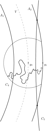
Figure 16: We show that, if starting at a distant point $w_{2}$, the probability of the simple random walk hitting $C_{4}\setminus A_{2}^{C}$ and the probability of hitting $C_{5}\cap A_{2}^{C}$ are comparable.

Let $y_{1}$ be the point on $\partial A_{2}$ closest to $y_{0}$. Let $C_{5}$ be a discrete ball of radius $h$ such that the intersection $C_{5}\cap\partial A_{2}$ has diameter $6s$ and center of mass as close as possible to $y_{1}$. By Donsker’s Invariance Principle, there is a constant $c_{1}>0$ such that a simple random walk started at any point in $\partial C_{4}\cap A_{2}^{C}$ has probability at least $c_{1}$ of reaching $C_{5}\cap\partial A_{2}$ before $\partial A_{2}\setminus C_{5}$. Let $w_{2}\in A_{2}^{C}$ be any point at distance at least $\frac{h}{2}$ from $y_{0}$. For a simple random walk starting at $w_{2}$ we define the events:

$D_{C_{5}\cap\partial A_{2}}:=\{H_{C_{5}\cap\partial A_{2}}\leq H_{\partial A_{2}\setminus C_{5}}\}$; the event where the simple random walk reaches $C_{5}\cap\partial A_{2}$ before reaching any other point in $\partial A_{2}$.

$D_{\partial C_{5}\cap A_{2}^{C}}:=\{H_{\partial C_{5}\cap A_{2}^{C}}\leq H_{\partial A_{2}\setminus C_{5}}\}$; the event where the simple random walk reaches $\partial C_{5}\cap A_{2}^{C}$ before reaching any other point in $\partial A_{2}$.

$D_{C_{4}\setminus A_{2}}:=\{H_{C_{4}\setminus A_{2}}\leq H_{\partial A_{2}\setminus C_{4}}\}$; the event where the simple random walk reaches $C_{4}\setminus A_{2}$ before reaching any other point in $\partial A_{2}$.

$D_{y_{0}}:=\{H_{y_{0}}\leq H_{\partial A_{2}}\}$; the event where the simple random walk reaches $y_{0}$ before hitting $\partial A_{2}$.

From the above discussion it is clear that:

(A.13) $$\mathbb{P}_{w_{2}}\big{[}D_{C_{5}\cap\partial A_{2}}\big{]}\leq\mathbb{P}_{w_{2}}\big{[}D_{\partial C_{5}\cap A_{2}^{C}}\big{]},$$

(A.14) $$\mathbb{P}_{w_{2}}\big{[}D_{y_{0}}\big{]}=\mathbb{P}_{w_{2}}\big{[}D_{y_{0}}\mid D_{C_{4}\setminus A_{2}}\big{]}\mathbb{P}_{w_{2}}\big{[}D_{C_{4}\setminus A_{2}}\big{]},$$

(A.15) $$\mathbb{P}_{w_{2}}\big{[}D_{C_{4}\setminus A_{2}^{C}}\big{]}\leq\frac{1}{c_{1}}\mathbb{P}_{w_{2}}\big{[}D_{C_{5}\cap\partial A_{2}}\big{]}.$$

Using Proposition 6.5.4 of [11] we can see that there is a constant $c>0$ such that

(A.16) $$\mathbb{P}_{w_{2}}\big{[}D_{\partial C_{5}\cap A_{2}^{C}}\big{]}\leq c\frac{s^{d-1}}{h^{d-1}}.$$

Collecting the estimates $(\ref{pathprobi},\ref{pathprobj},\ref{pathprobk},\ref{pathprobl})$, using the strong Markov property, and bounding

$$\mathbb{P}_{w_{2}}\big{[}D_{y_{0}}\mid~{}D_{C_{4}\setminus A_{2}}\big{]}$$

by the Green’s function estimate (2.1), we see that there is a constant $c>0$ such that

(A.17) $$\mathbb{P}_{w_{0}}\big{[}w_{0}\xrightarrow{2^{\prime}}y_{0}\big{]}\leq c\frac{s}{h}\cdot\frac{s^{d-1}}{h^{d-1}}s^{-(d-2)}=c\frac{s^{2}}{h^{d}}.$$

If $h<20s$ the result follows after using Green’s Function.

We also provide a lower bound for $\mathbb{P}_{w_{0}}\big{[}w_{0}\xrightarrow{2^{\prime}}y_{0}\big{]}$, which we will need later. Suppose $h\leq\frac{r}{2}$. Let $C_{3}^{\prime}$ be a discrete ball of radius $2h$ contained in $A_{2}^{C}$ that intersects $\partial A_{2}$ only at $w_{1}$. Let $C_{2}^{\prime}$ be a discrete ball of radius $\frac{h}{2}$ concentric with $C_{3}^{\prime}$. Let us describe an event of probability greater than $c_{1}\frac{s^{2}}{h^{d}}$, for some constant $c_{1}>0$, that is contained in $w_{0}\xrightarrow{2^{\prime}}y_{0}$. First the walk needs to hit $\partial C_{2}^{\prime}$ before hitting $\partial C_{3}^{\prime}$. The probability of such event is of order $\frac{s}{h}$, as can be seen using Lemma A.1. We will denote by $w_{2}$ the point in which the walk enters $\partial C_{2}^{\prime}$.

We define $C_{5}^{\prime}$ to be the discrete ball of radius $2h$ such that its center lies inside $A_{2}^{C}$ and the intersection $C_{5}^{\prime}\cap\partial A_{2}$ coincides with $C_{4}\cap\partial A_{2}$. In addition to all events defined in the proof of the upper bound for $\mathbb{P}_{w_{0}}\big{[}w_{0}\xrightarrow{2^{\prime}}y_{0}\big{]}$, we define the event, for a simple random walk starting in the interior of $C_{5}^{\prime}$:

$D_{\partial C_{5}^{\prime}\setminus A_{2}^{C}}:=\{H_{\partial C_{5}^{\prime}\setminus A_{2}^{C}}\leq H_{\partial A_{2}\setminus C_{5}^{\prime}}\}$; the event where the simple random walk started in the interior of $C_{5}^{\prime}$ reaches $\partial C_{5}^{\prime}\setminus A_{2}^{C}$ before reaching $\partial A_{2}\setminus C_{5}^{\prime}$.

We note that $w_{2}$ is in the interior of $C_{5}^{\prime}$ and that $D_{\partial C_{5}^{\prime}\setminus A_{2}^{C}}\subset D_{\partial C_{4}\setminus A_{2}}$. We then have:

(A.18) $$\begin{array}[]{e}\mathbb{P}_{w_{0}}\big{[}w_{0}\xrightarrow{2^{\prime}}y_{0}\big{]}&\geq&\sum_{w_{2}\in\partial C_{2}^{\prime}}\mathbb{P}_{w_{0}}\big{[}H_{\partial C_{2}^{\prime}}<H_{\partial C_{3}^{\prime}},X_{H_{\partial C_{2}^{\prime}}}=w_{2}\big{]}\mathbb{P}_{w_{2}}\big{[}D_{y_{0}}\big{]}\\ \hfil&=&\sum_{w_{2}\in\partial C_{2}^{\prime}}\mathbb{P}_{w_{0}}\big{[}H_{\partial C_{2}^{\prime}}<H_{\partial C_{3}^{\prime}},X_{H_{\partial C_{2}^{\prime}}}=w_{2}\big{]}\mathbb{P}_{w_{2}}\big{[}D_{y_{0}}\mid D_{C_{4}\setminus A_{2}}\big{]}\mathbb{P}_{w_{2}}\big{[}D_{C_{4}\setminus A_{2}}\big{]}\\ \hfil&\geq&\sum_{w_{2}\in\partial C_{2}^{\prime}}\mathbb{P}_{w_{0}}\big{[}H_{\partial C_{2}^{\prime}}<H_{\partial C_{3}^{\prime}},X_{H_{\partial C_{2}^{\prime}}}=w_{2}\big{]}\mathbb{P}_{w_{2}}\big{[}D_{y_{0}}\mid D_{C_{4}\setminus A_{2}}\big{]}\mathbb{P}_{w_{2}}\big{[}D_{\partial C_{5}^{\prime}\setminus A_{2}}\big{]}.\end{array}$$

Using Harnack’s Principle $($Theorem $6.3.9$ of [11]$)$ we are able to show the existence of a constant $c_{2}>0$ such that

(A.19) $$\mathbb{P}_{w_{2}}\big{[}D_{\partial C_{5}^{\prime}\setminus A_{2}}\big{]}\geq c_{2}\frac{s^{d-1}}{h^{d-1}}.$$

With this and $(\ref{pathprobp})$ we can find a constant $c_{1}>0$ such that

(A.20) $$\mathbb{P}_{w_{0}}\big{[}w_{0}\xrightarrow{2^{\prime}}y_{0}\big{]}\geq c_{1}\frac{s^{2}}{h^{d}}.$$

If $h\geq\frac{r}{2}$ we simply replace the balls $C_{3}^{\prime}$ and $C_{5}^{\prime}$ by $A_{2}^{C}$, the ball $C_{2}^{\prime}$ by a ball concentric with $A_{2}^{C}$ but with the diameter halves, and continue the proof identically.

$\boldsymbol{w\xrightarrow{4}y}$: Let $w_{3}$ be the closest point to $w$ in $\partial A_{2}$. Let $h_{4}$ be the Euclidean distance between $w$ and $y$, and suppose $h_{4}\leq\frac{r}{2}$. Let $C_{6}$ be a discrete ball of radius $2h_{4}$ contained in $A_{2}^{C}$ that intersects $\partial A_{2}$ only at $w_{3}$. Let $C_{7}$ be a discrete ball of radius $\frac{h_{4}}{2}$ concentric with $C_{6}$. Then again Lemma A.1 and some calculus show that the probability that a simple random walk started at $w$ will reach $\partial C_{7}$ before reaching $\partial C_{6}$ is less than the probability that the same walk will reach $\partial C_{7}$ before hitting $\partial A_{2}$ and bigger than $c_{1}\frac{s}{h_{4}}$, for some constant $c_{1}>0$.

Let $C_{8}$ be a discrete ball of radius $2h_{4}$ contained in $A_{2}^{C}$ that intersects $\partial A_{2}$ only at $y$. Let $y_{3}$ be a fixed point in $\partial C_{7}$. Then the probability that a simple random walk started at $y_{3}$ hits $y$ before hitting any other point in $\partial C_{8}$ is smaller than the probability that the same walk reaches $y$ before any other point in $\partial A_{2}$ and bigger than $\frac{c_{2}}{h_{4}^{d-1}}$, for some constant $c_{2}>0$, by the Harnack’s Principle $($Theorem $6.3.9$ of [11]$)$ and Lemma $6.3.7$ of [11]. Figure 17 illustrates the argument. Using the strong Markov property, we then have

(A.21) $$\mathbb{P}_{w_{0}}\big{[}w\xrightarrow{4}y\big{]}\geq c\frac{s}{h_{4}}h_{4}^{-(d-1)}.$$

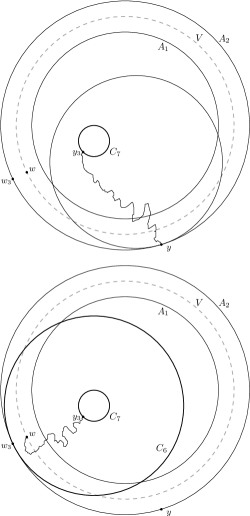
Figure 17: We can give a lower bound for $\mathbb{P}_{w_{0}}\big{[}w\xrightarrow{4}y\big{]}$ by describing the event where the walk started at $w$ reaches a small sphere $C_{6}$ before reaching $\partial C_{7}$ and then hits $y$ before any other point in $\partial C_{8}$.

If $h_{4}\geq\frac{r}{2}$ we simply replace the balls $C_{6}$ and $C_{8}$ by $A_{2}^{C}$, the ball $C_{7}$ by an discrete ball concentric with $A_{2}^{C}$ but with half the diameter, and continue the proof identically.

Let us now provide an upper bound for $\mathbb{P}_{w_{0}}\big{[}w\xrightarrow{4}y\big{]}$, which will be needed in the next section. We let $C_{6}^{\prime}$ be a discrete ball of radius $\frac{h_{4}}{6}$ lying outside $A_{2}^{C}$ and intersecting $\partial A_{2}$ only at $w_{3}$. We also let $C_{7}^{\prime}$ be a discrete ball of radius $\frac{h_{4}}{3}$ concentric with $C_{6}^{\prime}$. Finally we let $C_{8}^{\prime}$ be a discrete ball of radius $h_{4}$ lying outside $A_{2}^{C}$ and intersecting $\partial A_{2}$ only at $y$.

Then, for the simple random walk started at $w$ to hit $\partial A_{2}$ at $y$, it has first to reach $\partial C_{7}^{\prime}$ before hitting $\partial C_{6}^{\prime}$ and then hit $y$ before any other point in $\partial C_{8}^{\prime}$. As we have already seen, the probability of the first event is of order $\frac{s}{h_{4}}$ and the probability of the latter is of order $h_{4}^{-(d-1)}$. This way, we can find a constant $c>0$ such that:

(A.22) $$\mathbb{P}_{w_{0}}\big{[}w\xrightarrow{4}y\big{]}\leq c\frac{s}{h_{4}}h_{4}^{-(d-1)}.$$

Finally, using (A.12) and (A.13) we see that the supremum in (A.1) is reached when $h_{1}$ and $h_{3}$ are of order $s$. This way, $h$ should have the same order as $h_{4}$. Gathering the bounds (A.12), (A.13), (A.17) and (A.21) we have, for a constant $c>0$

(A.23) $$\sup_{\begin{subarray}{c}w\in V\\ y\in\partial A_{2}\end{subarray}}\mathbb{P}_{w}\big{[}w\xrightarrow{1}w_{0}\xrightarrow{2}y_{0}\xrightarrow{3}y\mid w\xrightarrow{4}y\big{]}\leq cs^{-2(d-1)}.$$

We have proved the following proposition:

Proposition A.2.

Regarding the sets $A_{1}^{\tiny\Circle},V^{\tiny\Circle}$ and $A_{2}^{\tiny\Circle}$, we have that, using the notation defined above, for some constants $c_{k}>0$, $k=1,\dots,9$, the following bounds are valid:

$$\mathbb{P}_{w}\big{[}w\xrightarrow{1}w_{0}\big{]}\leq c_{1}e^{\frac{-c_{2}h_{1}}{s}}s^{-(d-1)},$$

$$\mathbb{P}_{w}\big{[}y\xrightarrow{3}y_{0}\big{]}\leq c_{3}e^{\frac{-c_{4}h_{3}}{s}}s^{-(d-1)}s^{-1},$$

$$c_{5}\frac{s^{2}}{h^{d}}\leq\mathbb{P}_{w_{0}}\big{[}w_{0}\xrightarrow{2^{\prime}}y_{0}\big{]}\leq c_{6}\frac{s^{2}}{h^{d}},$$

$$c_{7}\frac{s}{h_{4}^{d}}\leq\mathbb{P}_{w_{0}}\big{[}w\xrightarrow{4}y\big{]}\leq c_{8}\frac{s}{h_{4}^{d}}.$$

$$\sup_{\begin{subarray}{c}w\in V\\ y\in\partial A_{2}\end{subarray}}\mathbb{P}_{w}\big{[}w\xrightarrow{1}w_{0}\xrightarrow{2}y_{0}\xrightarrow{3}y\mid w\xrightarrow{4}y\big{]}\leq c_{9}s^{-2(d-1)}.$$

A.1.2 The hanging probabilities for the smoothed hypercube

In this subsection we will focus on sets $A_{1}^{\tiny\Square},V^{\tiny\Square}$ and $A_{2}^{\tiny\Square}$, and the related simple random walk probabilities.

$\boldsymbol{w\xrightarrow{1}w_{0}}$: We will essentially use the same argument used when the underlying sets were balls. We assume without loss of generality that $\mathfrak{H}_{r+2s}$ is centered at the origin, and let $h_{1}:=\operatorname{dist}(w_{0},y_{0})$. We will subdivide the set $A_{2}^{C}\setminus A_{1}$ in sets of diameter of order $s$ in such a way that for a simple random walk trajectory started at $w$ to reach $w_{0}$ it will first have to cross a number of order $\frac{h_{1}}{s}$ of these sets.

Given $j\in\{1,\dots,d\}$, $(m_{1},\dots,m_{d})\in\{-1,1\}^{d}$, $k\in\{1,\dots,j-1,j+1,\dots,d\}$, and $i_{k}\in\{1,\dots,\big{\lfloor}\frac{r}{s}\big{\rfloor}\}$, we define

$$\begin{array}[]{e}E_{j,i_{1},\dots,i_{j-1},i_{j+1},\dots,i_{d}}^{(m_{1},\dots,m_{d})}&=&\Big{\{}(x_{1},\dots,x_{d})\in\mathbb{Z}^{d};\\ \hfil&\hfil&\quad x_{j}\in[\min\{m_{j}2^{-1}r,m_{j}(2^{-1}r+2s)\},\max\{m_{j}2^{-1}r,m_{j}(2^{-1}r+2s)\}],\\ \hfil&\hfil&\quad x_{k}\in[m_{k}(i_{k}-1)s,m_{k}i_{k}s]\cup[m_{k}i_{k}s,m_{k}(i_{k}-1)s].\Big{\}}\end{array}$$

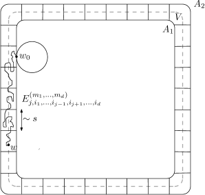
Figure 18: A path belonging to $w\xrightarrow{1}w_{0}$ has to cross $\frac{c_{1}h_{1}}{s}$ sets of the form $E_{j,i_{1},\dots,i_{j-1},i_{j+1},\dots,i_{d}}^{(m_{1},\dots,m_{d})}$ before hitting $w_{0}$ in $C_{1}^{\prime}$.

so that there exists a $c_{1}>0$ such that in order for the walk started at $w$ to hit $w_{0}$ in $A_{1}$, it will first have to cross at least $\big{\lfloor}\frac{c_{1}h_{1}}{s}\big{\rfloor}$ sets of the form $E_{j,i_{1},\dots,i_{j-1},i_{j+1},\dots,i_{d}}^{(m_{1},\dots,m_{d})}$. Each time the walk reaches a set $E_{j^{\prime},i_{1}^{\prime},\dots,i_{j-1}^{\prime},i_{j+1}^{\prime},\dots,i_{d}^{\prime}}^{(m_{1}^{\prime},\dots,m_{d}^{\prime})}$, the probability that it will reach another set of the form $E_{j,i_{1},\dots,i_{j-1},i_{j+1},\dots,i_{d}}^{(m_{1},\dots,m_{d})}$ at distance at least $s$ from $E_{j^{\prime},i_{1}^{\prime},\dots,i_{j-1}^{\prime},i_{j+1}^{\prime},\dots,i_{d}^{\prime}}^{(m_{1}^{\prime},\dots,m_{d}^{\prime})}$, before hitting either $\partial A_{1}$ or $\partial A_{2}$, is bounded from above by a constant $0<c_{2}<1$, as can be seen using Donsker’s Invariance Principle. Using the strong Markov property, we see that the probability that the walk started at $w$ crosses $\big{\lfloor}\frac{c_{1}h_{1}}{s}\big{\rfloor}$ sets of the form $E_{j,i_{1},\dots,i_{j-1},i_{j+1},\dots,i_{d}}^{(m_{1},\dots,m_{d})}$ is bounded from above by $c_{2}^{\lfloor\frac{c_{1}h_{1}}{s}\rfloor}$. See Figure 18.

Let $C_{1}^{\prime}$ be a discrete ball of radius $s$ contained in $A_{1}$ such that $C_{1}^{\prime}\cap\partial A_{1}~{}=~{}{w_{0}}$. Recall that the probability that a simple random walk started at a distance of order $s$ from $C_{1}^{\prime}$ will hit $C_{1}^{\prime}$ at $w_{0}$ is of order $s^{-(d-1)}$, and that it is harder for a walk started at $x\in A_{2}^{C}\setminus A_{1}$ to first hit $A_{1}$ at $w_{0}$ then it is for the same walk to first hit $C_{1}^{\prime}$ at $w_{0}$, that is,

$$\mathbb{P}_{x}\big{[}X_{H_{\partial A_{1}}}=w_{0}\big{]}\leq\mathbb{P}_{x}\big{[}X_{H_{\partial C_{1}^{\prime}}}=w_{0}\big{]}.$$

In conjunction with last paragraph’s argument and the strong Markov property, this shows the existence of a constant $c_{3},c_{4}>0$ such that

(A.24) $$\mathbb{P}_{w}\big{[}w\xrightarrow{1}w_{0}\big{]}\leq c_{3}e^{\frac{-c_{4}h_{1}}{s}}s^{-(d-1)}.$$

$\boldsymbol{y_{0}\xrightarrow{3}y}$: The proof of this bound is essentially the same as that of the corresponding bound in the case when the underlying sets are balls instead of smoothed hypercubes. We have, for some $c_{1},c_{2}>0$, and $h_{3}:=\operatorname{dist}(y,y_{0})$,

(A.25) $$\mathbb{P}_{w}\big{[}y\xrightarrow{3}y_{0}\big{]}\leq c_{1}e^{\big{\lfloor}\frac{-c_{2}h_{3}}{s}\big{\rfloor}}s^{-(d-1)}s^{-1}.$$

$\boldsymbol{w_{0}\xrightarrow{2^{\prime}}y_{0}}$: Let $h$ denote the Euclidean distance between $w_{0}$ and $y_{0}$. If $h<100s$, a simple application of the Green’s function bound gives the desired result. We then assume $h>100s$. Define $\tilde{B}_{x}$ to be the discrete ball in the $\ell_{\infty}$-norm centered in $x$ with radius $\frac{h}{4\sqrt{d}}$.

We will break up the path $\gamma_{2}^{0}\in w_{0}\xrightarrow{2^{\prime}}y_{0}$ in pieces that are easier to work with. Let $w_{4}\in\partial\tilde{B}_{w_{0}}\cap A_{2}^{C}$, $y_{4}\in\partial\tilde{B}_{y_{0}}\cap A_{2}^{C}$. We define the collection of finite paths:

• $w_{0}\xrightarrow{5}w_{4}$: The collection of all finite nearest-neighbor paths starting at $w_{0}$ whose only intersection with $\partial\tilde{B}_{w_{0}}\cup\partial A_{2}$ is at its ending point $w_{4}\in\partial\tilde{B}_{w_{0}}\cap A_{2}^{C}$. It is straightforward to see this collection as a simple random walk event.
  

• $w_{4}\xrightarrow{6}y_{4}$: The collection of finite nearest-neighbor paths starting at $w_{4}$ and ending at $y_{4}$, without intersecting $\partial A_{2}$.
  

• $y_{4}\xrightarrow{7}y_{0}$: The collection of all finite nearest-neighbor paths that start at $y_{4}$, never return to $\partial\tilde{B}_{y_{0}}\cap A_{2}^{C}$, and end at $y_{0}$ without ever reaching $\partial A_{2}$. It is simple to see this collection as a simple random walk event.

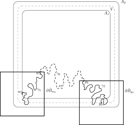
Figure 19: Definition of the paths $\gamma_{5}$, $\gamma_{6}$ and $\gamma_{7}$.

As before, we denote by $w_{0}\xrightarrow{5}w_{4}\xrightarrow{6}y_{4}\xrightarrow{7}y_{0}$ the concatenation of these three collections.

Analogously to what we noted at the start of this section, we observe that $\gamma_{2}^{0}\in w_{0}\xrightarrow{2^{\prime}}y_{0}$ if and only if there exists $w_{4}\in\partial\tilde{B}_{w_{0}}\cap A_{2}^{C}$ and $y_{4}\in\partial\tilde{B}_{y_{0}}\cap A_{2}^{C}$ such that $\gamma_{2}^{0}$ is the concatenation of three paths: $\gamma_{5}\in w_{0}\xrightarrow{5}w_{4}$, $\gamma_{6}\in w_{4}\xrightarrow{6}y_{4}$, and $\gamma_{7}\in y_{4}\xrightarrow{7}y_{0}$.

We also define

• $w_{4}\xrightarrow{6^{\prime}}y_{4}$ The collection of finite simple random walk trajectories starting at $w_{4}$ and ending at its first visit to $y_{4}$ without intersecting $\partial A_{2}$. This collection can also be seen as the event where the simple random walk started at $w_{4}$ visits $y_{4}$ before it hits $\partial A_{2}$.

Using the same trick we used to obtain the bound (A.6), we can find a constant $c>1$ such that

(A.26) $$\mathbb{P}_{w_{4}}\big{[}w_{4}\xrightarrow{6^{\prime}}y_{4}\big{]}\leq\sum_{\gamma_{6}\in w_{4}\xrightarrow{6}y_{4}}\frac{1}{2^{|\gamma_{6}|}}\leq c\mathbb{P}_{w_{4}}\big{[}w_{4}\xrightarrow{6^{\prime}}y_{4}\big{]}.$$

We then have

$$\mathbb{P}_{w_{0}}\big{[}w_{0}\xrightarrow{2^{\prime}}y_{0}\big{]} =\sum_{\begin{subarray}{c}w_{4}\in\partial\tilde{B}_{w_{0}}\cap A_{2}^{C}\\ \gamma_{5}\in w_{0}\xrightarrow{5}w_{4}\end{subarray}}\frac{1}{2^{|\gamma_{5}|}}\sum_{\begin{subarray}{c}y_{4}\in\partial\tilde{B}_{y_{0}}\cap A_{2}^{C}\\ \gamma_{6}\in w_{4}\xrightarrow{6}y_{4}\end{subarray}}\frac{1}{2^{|\gamma_{6}|}}\sum_{\gamma_{7}\in y_{4}\xrightarrow{6}y_{0}}\frac{1}{2^{|\gamma_{7}|}}$$

(A.27) $$\leq c\sum_{w_{4}}\mathbb{P}_{w_{0}}\big{[}w_{0}\xrightarrow{5}w_{4}\big{]}\sum_{y_{4}}\mathbb{P}_{w_{4}}\big{[}w_{4}\xrightarrow{6^{\prime}}y_{4}\big{]}\mathbb{P}_{y_{4}}\big{[}y_{4}\xrightarrow{7}y_{0}\big{]}.$$

We then use the Green’s function estimate (2.1) to bound $\mathbb{P}_{w_{4}}\big{[}w_{4}\xrightarrow{6^{\prime}}y_{4}\big{]}$ by $ch^{d-2}$ (note that $\operatorname{dist}(w_{4},y_{4})=O(h)$). Using this bound on the above equality, we obtain

(A.28) $$\mathbb{P}_{w_{0}}\big{[}w_{0}\xrightarrow{2^{\prime}}y_{0}\big{]}\leq ch^{d-2}\sum_{w_{4}}\mathbb{P}_{w_{0}}\big{[}w_{0}\xrightarrow{5}w_{4}\big{]}\sum_{y_{4}}\mathbb{P}_{y_{4}}\big{[}y_{4}\xrightarrow{7}y_{0}\big{]}.$$

We define the events

• $w_{0}\xrightarrow{5}\partial\tilde{B}_{w_{0}}$: The event where the simple random walk started at $w_{0}$ reaches $\partial\tilde{B}_{w_{0}}$ before reaching $\partial A_{2}$.
  

• $y_{0}\xrightarrow{5}\partial\tilde{B}_{y_{0}}$: The event where the simple random walk started at $y_{0}$ reaches $\partial\tilde{B}_{y_{0}}$ before reaching $\partial A_{2}$.

Note that

(A.29) $$\sum_{w_{4}}\mathbb{P}_{w_{0}}\big{[}w_{0}\xrightarrow{5}w_{4}\big{]}=\mathbb{P}_{w_{0}}\big{[}w_{0}\xrightarrow{5}\partial\tilde{B}_{w_{0}}\big{]},$$

and using the simple random walk’s reversibility, we also have

(A.30) $$\sum_{y_{4}}\mathbb{P}_{y_{4}}\big{[}y_{4}\xrightarrow{5}y_{0}\big{]}=\mathbb{P}_{y_{0}}\big{[}y_{0}\xrightarrow{5}\partial\tilde{B}_{y_{0}}\big{]},$$

so that we obtain the following bound

(A.31) $$\mathbb{P}_{w_{0}}\big{[}w_{0}\xrightarrow{2^{\prime}}y_{0}\big{]}\leq\frac{c}{h^{d-2}}\mathbb{P}_{w_{0}}\big{[}w_{0}\xrightarrow{5}\partial\tilde{B}_{w_{0}}\big{]}\mathbb{P}_{y_{0}}\big{[}y_{0}\xrightarrow{5}\partial\tilde{B}_{y_{0}}\big{]}.$$

We still have to obtain a bound for these last two probabilities. Since they are similarly defined, the bound for both of them follows from the same arguments, and thus we will only provide a bound for $\mathbb{P}_{w_{0}}\big{[}w_{0}\xrightarrow{5}\partial\tilde{B}_{w_{0}}\big{]}$.

We will do so by looking at the projections of the random walk trajectory in each of the $d$ orthogonal axes. Since we will need to look at these projections independently, we will change our object of study from the simple random walk on $\mathbb{Z}^{d}$ to the continuous time simple random walk on $\mathbb{Z}^{d}$ with waiting times between steps distributed as $\mathop{\mathrm{Exp}}(1)$ random variables. Since we will be studying properties of the random walk’s trajectories, this change of framework will in no way impact the probabilities of interest. We will denote by $\mathbb{P}_{x}^{c}$, with $x\in\mathbb{Z}^{d}$, the probability measure associated with such continuous time random walk starting at $x$.

We recall the definition of $\mathfrak{H}_{r+2s}$, the unsmoothed version of $A_{2}^{C}$. Here we will assume $\mathfrak{H}_{r+2s}$ takes the form

$$\mathfrak{H}_{r+2s}:=\big{\{}(x_{1},\dots,x_{d})\in\mathbb{Z}^{d}:0\leq x_{i}\leq r+2s,\text{ for all }i=1,\dots,d\big{\}}$$

Without loss of generality we assume that $0\in\mathbb{Z}^{d}$ is the point belonging to $\{0,r+2s\}^{d}$ which is closest to $w_{0}$. We denote $w_{0}\equiv(w_{0}^{1},\dots,w_{0}^{d})$ and for each $j\in\{1,\dots,d\}$ we let $(X_{t}^{j},t\geq 0)$ be the projection on the $j$-th axis of the continuous time random walk started at $w_{0}$. This projection is itself a continuous time random walk started at $w_{0}^{j}$ with waiting time between jumps given by a $\mathop{\mathrm{Exp}}(d)$ random variable, and, as we already noted, these random walks are independent from each other. We will define $\mathbb{P}^{j}_{x}$ to be the probability measure associated with this projected random walk when it starts at $x\in\mathbb{Z}$.

We define, for $j\in\{1,\dots,d\}$ and $A\subset\mathbb{Z}$ , the hitting times

(A.32) $$\tau^{j}(A) :=\inf_{t\geq 0}\{X^{j}_{t}\in A\},$$

(A.33) $$\tau^{j} :=\tau^{j}(\{\max\{0,w_{0}^{j}-h\},w_{0}^{j}+h\}),$$

and we let $J_{t}^{j}$ denote the number of jumps the continuous time walk projected on the $j$-th direction makes before time $t$.

Since $J_{t}^{j}$ has Poisson distribution with parameter $td^{-1}$, we have (using a convenient large deviation estimate):

(A.34) $$\mathbb{P}_{\!w_{0}^{j}}^{j}\Bigg{[}\frac{(1-\delta)t}{d}\leq J^{j}_{t}\leq\frac{(1+\delta)t}{d}\Bigg{]}\geq 1-e^{c(\delta)t}.$$

Given $w_{0}$, we divide the $d$ directions of $\mathbb{Z}^{d}$ in two kinds. The first kind will be such that $\max\{0,w_{0}^{j}-h\}=0$, the second will be such that $\max\{0,w_{0}^{j}-h\}=w_{0}^{j}-h$. We assume without loss of generality the first $d_{0}$ directions to be of the first kind and the remaining directions to be of the second kind.

Given $t\in\mathbb{R}_{+}$, we will need to bound the probability $\mathbb{P}_{\!w_{0}^{j}}^{j}\big{[}\tau^{j}>t\big{]}$. We first assume $j\leq d_{0}$. We denote by $(S^{x}_{k},k\in\mathbb{Z}_{+})$ the unidimensional discrete time simple random walk starting at $x\in\mathbb{Z}$, and by $\mathbb{P}_{x}^{\mathbb{Z}}$ its associated measure. We have

(A.35) $$\mathbb{P}_{\!w_{0}^{j}}^{j}\big{[}\tau^{j}>t\big{]}\leq\mathbb{P}_{\!w_{0}^{j}}^{j}\big{[}\tau^{j}_{\{0\}}>t\big{]}\leq\sum_{t_{0}}\mathbb{P}_{\!w_{0}^{j}}^{\mathbb{Z}}\big{[}\min_{0\leq k\leq t_{0}}S_{k}^{w_{0}^{j}}>0\big{]}\mathbb{P}_{\!w_{0}^{j}}^{c}\big{[}J_{t}^{j}=t_{0}\big{]}.$$

Using (A.34), the reflection principle for the unidimensional simple random walk, and the central limit theorem, we can bound the above expression by

(A.36) $$\sum_{\begin{subarray}{c}t_{0}\in\mathbb{Z}_{+},\\ t_{0}\in\big{(}\frac{(1-\delta)t}{d},\frac{(1+\delta)t}{d}\big{)}\end{subarray}}\mathbb{P}_{\!w_{0}^{j}}^{c}\big{[}J_{t}^{j}=t_{0}\big{]}\Big{(}1-2\mathbb{P}_{\!w_{0}^{j}}^{\mathbb{Z}}\big{[}S_{t_{0}}^{w_{0}^{j}}<0\big{]}\Big{)}+e^{-c(\delta)t}$$

$$=\sum_{\begin{subarray}{c}t_{0}\in\big{(}\frac{(1-\delta)t}{d},\frac{(1+\delta)t}{d}\big{)}\end{subarray}}\mathbb{P}_{\!w_{0}^{j}}^{c}\big{[}J_{t}^{j}=t_{0}\big{]}\Big{(}1-2\mathbb{P}_{0}^{\mathbb{Z}}\big{[}S_{t_{0}}^{0}>w_{0}^{j}\big{]}\Big{)}+e^{-c(\delta)t}$$

$$\leq c\sum_{\begin{subarray}{c}t_{0}\in\mathbb{Z}_{+},\\ t_{0}\in\big{(}\frac{(1-\delta)t}{d},\frac{(1+\delta)t}{d}\big{)}\end{subarray}}\mathbb{P}_{\!w_{0}^{j}}^{c}\big{[}J_{t}^{j}=t_{0}\big{]}\Big{(}1-\frac{2}{\sqrt{2\pi}}\int_{0}^{\infty}e^{-\frac{v^{2}}{2}}\mathrm{d}v$$

(A.37) $$\quad\quad\quad+\quad\frac{2}{\sqrt{2\pi}}\int_{0}^{\frac{w_{0}^{j}}{\sqrt{t_{0}}}}e^{-\frac{v^{2}}{2}}\mathrm{d}v+O(\sqrt{t_{0}})^{-1}\Big{)}+e^{-c(\delta)t}$$

$$\leq c\sum_{\begin{subarray}{c}t_{0}\in\mathbb{Z}_{+},\\ t_{0}\in\big{(}\frac{(1-\delta)t}{d},\frac{(1+\delta)t}{d}\big{)}\end{subarray}}\mathbb{P}_{\!w_{0}^{j}}^{c}\big{[}J_{t}^{j}=t_{0}\big{]}\frac{w_{0}^{j}}{\sqrt{t_{0}}}$$

$$\leq c\frac{w_{0}^{j}}{\sqrt{t}}.$$

In a analogous way, we show for $j>d_{0}$

(A.38) $$\mathbb{P}_{\!w_{0}^{j}}^{j}\big{[}\tau^{j}>t\big{]}\leq c\frac{h}{\sqrt{t}}.$$

We now bound the probability that the walk exits the sphere $\partial\tilde{B}_{w_{0}}$ through the first direction, without ever hitting $\partial A_{2}$.

(A.39) $$\mathbb{P}_{w_{0}}^{c}\big{[}X_{\tau^{1}}^{1}=w_{0}^{1}+h,\tau^{j}>\tau^{1}\text{ for all }j\neq 1\big{]}$$

$$=\mathbb{P}_{\!w_{0}^{1}}^{1}\big{[}X_{\tau^{1}}^{1}=w_{0}^{1}+h\big{]}\int\prod_{j\neq 1}\mathbb{P}_{\!w_{0}^{j}}^{j}\big{[}\tau^{j}>t\big{]}\mathbb{P}_{w_{0}}^{c}\big{[}\tau^{1}=t+\mathrm{d}t\mid X_{\tau^{1}}^{1}=w_{0}^{1}+h\big{]},$$

where $\mathbb{P}_{w_{0}}^{c}\big{[}\tau^{1}=t+\mathrm{d}t\mid X_{\tau^{1}}^{1}=w_{0}^{1}+h\big{]}$ is the distribution of $\tau^{1}$ conditioned on the event $\{X_{\tau^{1}}^{1}=w_{0}^{1}+h\}$. Then, using $(\ref{tau1})$, $(\ref{tau2})$ and the gambler’s ruin estimate (see Section $5.1$ of [11]), we are able to bound the above expression by

(A.40) $$c\frac{w_{0}^{1}}{h}\int\prod_{1<j\leq d_{0}}\frac{w_{0}^{j}}{\sqrt{t}}\prod_{d_{0}<j\leq d}\frac{h}{\sqrt{t}}\mathbb{P}_{w_{0}}^{c}\big{[}\tau^{1}=t+\mathrm{d}t\mid X_{\tau^{1}}^{1}=w_{0}^{1}+h\big{]}.$$

We define the continuous time simple random walk

(A.41) $$X_{t}^{1,\frac{1}{2}}:=X^{1}_{t+\tau^{1}(\{0,\lceil 2^{-1}(w_{0}^{1}+h)\rceil\})},$$

so that, on $\{X_{\tau^{1}}^{1}=w_{0}^{1}+h\}$, $X_{t}^{1,\frac{1}{2}}$ is distributed as a continuous time one-dimensional walk starting at a halfway point between $0$ and $w_{0}^{1}+h$. We also define the hitting time

(A.42) $$\tau^{1,\frac{1}{2}}:=\inf\{t\geq 0;X_{t}^{1,\frac{1}{2}}\in\{0,w_{0}^{1}+h\}\}.$$

On the event $\{X_{\tau^{1}}^{1}=w_{0}^{1}+h\}$, $\tau^{1}$ is distributed as $\tau^{1}(\{0,\lceil 2^{-1}(w_{0}^{1}+h)\rceil\})+\tau^{1,\frac{1}{2}}$, so that $\{\tau^{1}<t\}$ implies $\{\tau^{1,\frac{1}{2}}<t\}$.

We then have, for $\alpha<1$

(A.43) $$\mathbb{P}_{w_{0}}^{c}\Big{[}\tau^{1}<\alpha h^{2}d\mid X_{\tau^{1}}^{1}=w_{0}^{1}+h\Big{]}\leq\mathbb{P}_{w_{0}}^{c}\Big{[}\tau^{1,\frac{1}{2}}<\alpha h^{2}d\mid X_{\tau^{1}}^{1}=w_{0}^{1}+h\Big{]}.$$

Since $X_{t}^{1,\frac{1}{2}}$ starts at a halfway point between $0$ and $w_{0}^{1}+h$, we have

(A.44) $$\mathbb{P}_{w_{0}}^{c}\Big{[}\tau^{1,\frac{1}{2}}<\alpha h^{2}d\mid X_{\tau^{1}}^{1}=w_{0}^{1}+h\Big{]}\leq c\mathbb{P}_{2^{-1}(w_{0}^{1}+h)}^{1}\Big{[}\tau^{1,\frac{1}{2}}<\alpha h^{2}d\Big{]}.$$

Using (A.34) together with a large deviation estimate (see Lemma $1.5.1$ of [10]), we obtain

(A.45) $$\mathbb{P}_{w_{0}}^{c}\big{[}\tau^{1}<\alpha h^{2}d\mid X_{\tau^{1}}^{1}=w_{0}^{1}+h\big{]}\leq e^{c\alpha^{-1}}.$$

We define

(A.46) $$\psi_{w_{0}}(t):=c\frac{w_{0}^{1}}{h}\prod_{1<j\leq d_{0}}\frac{w_{0}^{j}}{\sqrt{t}}\prod_{d_{0}<j\leq d}\frac{h}{\sqrt{t}}.$$

Then

$$\mathbb{P}_{w_{0}}^{c}\big{[}X_{\tau^{1}}^{1}=w_{0}^{1}+h,\tau^{j}>\tau^{1}\text{ for all }j\neq 1\big{]}$$*****

$$\leq c\frac{w_{0}^{1}}{h}\int\prod_{1<j\leq d_{0}}\frac{w_{0}^{j}}{\sqrt{t}}\prod_{d_{0}<j\leq d}\frac{h}{\sqrt{t}}\mathbb{P}_{w_{0}}^{c}\big{[}\tau^{1}=t+\mathrm{d}t\mid X_{\tau^{1}}^{1}=w_{0}^{1}+h\big{]}$$

$$=\sum_{k\geq 1}c\frac{w_{0}^{1}}{h}\int_{t=h^{2}d(k+1)^{-1}}^{t=h^{2}dk^{-1}}\prod_{1<j\leq d_{0}}\frac{w_{0}^{j}}{\sqrt{t}}\prod_{d_{0}<j\leq d}\frac{h}{\sqrt{t}}\mathbb{P}_{w_{0}}^{c}\big{[}\tau^{1}=t+\mathrm{d}t\mid X_{\tau^{1}}^{1}=w_{0}^{1}+h\big{]}$$

$$\quad+c\frac{w_{0}^{1}}{h}\int_{t\geq h^{2}d}\prod_{1<j\leq d_{0}}\frac{w_{0}^{j}}{\sqrt{t}}\prod_{d_{0}<j\leq d}\frac{h}{\sqrt{t}}\mathbb{P}_{w_{0}}^{c}\big{[}\tau^{1}=t+\mathrm{d}t\mid X_{\tau^{1}}^{1}=w_{0}^{1}+h\big{]}$$

$$\leq\psi_{w_{0}}(h^{2}d)+\sum_{k\geq 1}\psi_{w_{0}}(h^{2}dk^{-1})e^{-ck}.$$

Since $\psi_{w_{0}}(h^{2}dk^{-1})$ grows polynomially in $k$ as $k\rightarrow\infty$, we have

(A.47) $$\mathbb{P}_{w_{0}}^{c}\big{[}X_{\tau^{1}}^{1}=w_{0}^{1}+h,\tau^{j}>\tau^{1}\text{ for all }j\neq 1\big{]}\leq c\psi_{w_{0}}(h^{2}d)\leq c^{\prime}\prod_{1\leq j\leq d_{0}}\frac{w_{0}^{j}}{h}.$$

The proof is analogous for every $j=1,\dots,d$. When $j>d_{0}$ the calculations are in fact easier because, since $\max\{0,w_{0}^{j}-h\}=w_{0}^{j}-h$, there is no preferential direction in which the random walk $(X^{j}_{t},t\geq 0)$ has to exit the ball $\partial\tilde{B}_{w_{0}}\cap A_{2}^{C}$, so that the required conditioning in $(\ref{condcontwalk})$ is simpler. We then have, for $j$ such that $d_{0}<j\leq d$,

(A.48) $$\mathbb{P}_{w_{0}}^{c}\big{[}\tau^{n}>\tau^{j}\text{ for all }n\neq j\big{]}\leq c\prod_{1\leq j\leq d_{0}}\frac{w_{0}^{j}}{h},$$

so that

(A.49) $$\mathbb{P}\big{[}w_{0}\xrightarrow{5}\partial\tilde{B}_{w_{0}}\big{]} \leq\sum_{1\leq k\leq d_{0}}\mathbb{P}_{w_{0}}^{c}\big{[}X_{\tau^{k}}^{k}=w_{0}^{k}+h,\tau^{n}>\tau^{k}\text{ for all }n\neq j\big{]}$$

$$\quad+\sum_{d_{0}<k\leq d}\mathbb{P}_{w_{0}}^{c}\big{[}\tau^{n}>\tau^{k}\text{ for all }n\neq j\big{]}$$

$$\leq c\prod_{1\leq i\leq d_{0}}\frac{w_{0}^{i}}{h}.$$

We will change the notation so that we are able to express the inequality above in a way that does not uses the fact that $\{0\}^{d}$ is the vertex of $\{0,r+2s\}^{d}$ which is closest to $w_{0}$. Let $\mathfrak{H}^{d-1}_{i}$; $i=1,\dots,2d$; denote the $(d-1)$-dimensional hyperfaces of $\mathfrak{H}_{r+2s}$, and let $l^{w_{0}}_{i}:=\min\{\operatorname{dist}(w_{0},\mathfrak{H}^{d-1}_{i}),h\}$, and $l^{y_{0}}_{i}:=\min\{\operatorname{dist}(y_{0},\mathfrak{H}^{d-1}_{i}),h\}$. Then, (A.49) implies

$$\mathbb{P}\big{[}w_{0}\xrightarrow{5}\partial\tilde{B}_{w_{0}}\big{]}\leq c\frac{l^{w_{0}}_{1}\dots l^{w_{0}}_{2d}}{h^{2d}},$$

and using the same arguments used above, we can see that

$$\mathbb{P}\big{[}y_{0}\xrightarrow{5}\partial\tilde{B}_{y_{0}}\big{]}\leq c\frac{l^{y_{0}}_{1}\dots l^{y_{0}}_{2d}}{h^{2d}}.$$

Together with (A.31), this shows

(A.50) $$\mathbb{P}_{w_{0}}\big{[}w_{0}\xrightarrow{2^{\prime}}y_{0}\big{]}\leq ch^{-(d-2)}\frac{l^{w_{0}}_{1}\dots l^{w_{0}}_{2d}}{h^{2d}}\frac{l^{y_{0}}_{1}\dots l^{y_{0}}_{2d}}{h^{2d}}.$$

We will also need a matching lower bound. We will continue to use the same notations and conventions. Again we assume $h>100s$, since otherwise the lower bound follows immediately from using a Green’s function estimate. We define

(A.51) $$w_{5}:=\Big{(}w_{0}^{1}+\frac{h}{4\sqrt{d}},\dots,w_{0}^{d_{0}}+\frac{h}{4\sqrt{d}},w_{0}^{d_{0}+1},\dots,w_{0}^{d}\Big{)},$$

We analogously define $y_{5}$: Let $e_{i_{d_{1}}},\dots,e_{i_{d_{k}}}$ be the vectors in the orthonormal basis of $\mathbb{R}^{d}$ corresponding to the directions in which the ball $B_{\infty}\big{(}y_{0},\frac{h}{4\sqrt{d}}\big{)}$ passes the limits of the hypercube $\mathfrak{H}_{r+2s}$. $y_{5}$ is defined to be the point in $A_{2}^{C}$ such that

$$l=d_{1},\dots,d_{k}\implies|\langle y_{5}-y_{0},e_{i_{l}}\rangle|=\frac{h}{4\sqrt{d}},$$

$$n\neq d_{1},\dots,d_{k}\implies|\langle y_{5}-y_{0},e_{i_{n}}\rangle|=0$$

and

$$B_{\infty}\Big{(}y_{5},\frac{h}{4\sqrt{d}}\Big{)}\subseteq\mathfrak{H}_{r+2s}.$$

Our plan is to describe an event contained in $w_{0}\xrightarrow{2^{\prime}}y_{0}$ with probability matching that of the right side of $(\ref{2final})$. We let

$$B_{w_{5}}:=B_{\infty}\Big{(}w_{5},\frac{h}{16\sqrt{d}}\Big{)},$$

and

$$B_{y_{5}}:=B_{\infty}\Big{(}y_{5},\frac{h}{16\sqrt{d}}\Big{)},$$

For $w_{6}\in\partial B_{w_{5}}$ and $y_{6}\in\partial B_{y_{5}}$, we define the events

• $w_{0}\xrightarrow{8}w_{6}$: The event where the random walk started at $w_{0}$ hits $\partial B_{w_{5}}$ before hitting $\partial A_{2}$ and its entrance point in $\partial B_{w_{5}}$ is $w_{6}$.
  

• $w_{6}\xrightarrow{9}y_{6}$: The event where the random walk started at $w_{6}$ visits $y_{6}\in\partial B_{y_{5}}$ before reaching $\partial A_{2}$.
  

• $y_{6}\xrightarrow{10}y_{0}$: The event where the simple random walk started at $y_{6}$ hits $y_{0}$ before returning to $\partial B_{y_{5}}$.

Figure 20: Definition of the paths $\gamma_{8}$, $\gamma_{9}$ and $\gamma_{10}$.

And we denote by $w_{0}\xrightarrow{8}w_{6}\xrightarrow{9}y_{6}\xrightarrow{10}y_{0}$ the “concatenation” of these three events, that is, the path $\gamma$ belongs to the event $w_{0}\xrightarrow{8}w_{6}\xrightarrow{9}y_{6}\xrightarrow{10}y_{0}$ if and only if $\gamma$ is the concatenation of three paths: $\gamma_{8}\in w_{0}\xrightarrow{8}w_{6}$, $\gamma_{9}\in w_{6}\xrightarrow{9}y_{6}$ and $\gamma_{10}\in y_{6}\xrightarrow{10}y_{0}$. It is then clear that

$$\bigcup_{w_{6}}\bigcup_{y_{6}}w_{0}\xrightarrow{8}w_{6}\xrightarrow{9}y_{6}\xrightarrow{10}y_{0}\subset w_{0}\xrightarrow{2^{\prime}}y_{0},$$

so that; summing over $\gamma_{8}\in w_{0}\xrightarrow{8}w_{6}$, $\gamma_{9}\in w_{6}\xrightarrow{9}y_{6}$ and $\gamma_{10}\in y_{6}\xrightarrow{10}y_{0}$; we have

(A.52) $$\begin{array}[]{e}\mathbb{P}_{w_{0}}\big{[}w_{0}\xrightarrow{2^{\prime}}y_{0}\big{]}&\geq&\sum_{w_{6}}\sum_{\gamma_{8}}\frac{1}{2^{|\gamma_{8}|}}\sum_{y_{6}}\sum_{\gamma_{9}}\frac{1}{2^{|\gamma_{9}|}}\sum_{\gamma_{10}}\frac{1}{2^{|\gamma_{10}|}}\\[14.22636pt] \hfil&=&\sum_{w_{6}}\mathbb{P}_{w_{0}}\big{[}w_{0}\xrightarrow{8}w_{6}\big{]}\sum_{y_{6}}\mathbb{P}_{w_{6}}\big{[}w_{6}\xrightarrow{9}y_{6}\big{]}\mathbb{P}_{y_{6}}\big{[}y_{6}\xrightarrow{10}y_{0}\big{]}\\[14.22636pt] \hfil&\geq&\frac{c}{h^{d-2}}\sum_{w_{6}}\mathbb{P}_{w_{0}}\big{[}w_{0}\xrightarrow{8}w_{6}\big{]}\sum_{y_{6}}\mathbb{P}_{y_{6}}\big{[}y_{6}\xrightarrow{10}y_{0}\big{]},\end{array}$$

where we bounded $\mathbb{P}_{w_{6}}\big{[}w_{6}\xrightarrow{9}y_{6}\big{]}$ from below by $ch^{d-2}$ using the Green’s function estimate (2.1) and the fact that the distance of both $w_{6}$ and $y_{6}$ from $\partial A_{2}$ has order $h$.

We define the events

• $w_{0}\xrightarrow{8}\partial B_{w_{5}}$: The event where the simple random walk started at $w_{0}$ reaches $\partial B_{w_{5}}$ before reaching $\partial A_{2}$.
  

• $y_{0}\xrightarrow{8}\partial B_{y_{5}}$: The event where the simple random walk started at $y_{0}$ reaches $\partial B_{y_{5}}$ before reaching $\partial A_{2}$.

Due to the simple random walk’s reversibility, we get that

(A.53) $$\mathbb{P}_{w_{0}}\big{[}w_{0}\xrightarrow{2^{\prime}}y_{0}\big{]}\geq\frac{c}{h^{d-2}}\mathbb{P}_{w_{0}}\big{[}w_{0}\xrightarrow{8}\partial B_{w_{5}}\big{]}\mathbb{P}_{y_{0}}\big{[}y_{0}\xrightarrow{10}\partial B_{y_{5}}\big{]}.$$

We will prove a bound for $\mathbb{P}_{w_{0}}\big{[}w_{0}\xrightarrow{8}\partial B_{w_{5}}\big{]}$, since the bound for $\mathbb{P}_{y_{0}}\big{[}y_{0}\xrightarrow{10}\partial B_{y_{5}}\big{]}$ follows from analogous arguments. We will use the same continuous time random walk projections to study this probability. The notation used will be the same as the one used in the proof of the upper bound. For $1\leq j\leq d_{0}$, we define

$$\tau^{j}:=\inf\Bigg{\{}t\geq 0,X^{j}_{t}\in\Big{\{}0,w_{0}^{j}+\frac{h}{4\sqrt{d}}\Big{\}}\Bigg{\}},$$

and on the event $\big{\{}X^{j}_{\tau^{j}}=w_{0}^{j}+\frac{h}{4\sqrt{d}}\big{\}}$, we define $\tau^{j}_{\infty}$ as

$$\tau^{j}_{\infty}:=\inf\Bigg{\{}t\geq 0,X^{j}_{t+\tau^{j}}\in\Big{\{}w_{0}^{j}+\frac{3h}{16\sqrt{d}},w_{0}^{j}+\frac{5h}{16\sqrt{d}}\Big{\}}\Bigg{\}},$$

that is, the first time after $\tau^{j}$ when the projection of the continuous time simple random walk on the $j$-th direction hits the projected boundary of the ball $B_{w_{5}}$. For $d_{0}<m\leq d$, we also define

$$\tau^{m}_{\infty}:=\inf\Bigg{\{}t\geq 0,X^{m}_{t}\in\Big{\{}w_{0}^{m}-\frac{h}{16\sqrt{d}},w_{0}^{m}+\frac{h}{16\sqrt{d}}\Big{\}}\Bigg{\}},$$

the first time the walk projected in the $m$-th direction hits the projected boundary of the ball $B_{w_{5}}$. Finally, we define

$$T:=\max_{1\leq i\leq d_{0}}\tau^{i}.$$

We then have, for any $l>0$,

$$\mathbb{P}_{w_{0}}\Big{[}w_{0}\xrightarrow{8}\partial B_{w_{5}}\Big{]}$$****

$$\geq\mathbb{P}_{w_{0}}^{c}\left[\begin{array}[]{c}X^{j}_{\tau^{j}}=w_{0}^{j}+\frac{h}{4\sqrt{d}},\tau^{j}_{\infty}>T\text{ for all }j=1,\dots,d_{0}\phantom{*};\\ \tau^{m}_{\infty}>T\text{ for all }m=d_{0}+1,\dots,d\end{array}\right]$$

$$\geq\mathbb{P}_{w_{0}}^{c}\Big{[}T<l\Big{]}\prod_{1\leq j\leq d_{0}}\mathbb{P}_{\!w_{0}^{j}}^{j}\Big{[}X^{j}_{\tau^{j}}=w_{0}^{j}+\frac{h}{4\sqrt{d}},\tau^{j}_{\infty}>l\Big{]}\prod_{d_{0}<m\leq d}\mathbb{P}_{\!w_{0}^{m}}^{m}\Big{[}\tau^{m}_{\infty}>l\Big{]}.$$

Now, let $c_{1},c_{2}>0$ be such that $c_{1}>c_{2}$. We have that

$$\mathbb{P}_{w_{0}}^{c}\big{[}T<c_{1}h^{2}\big{]}\geq c>0.$$

For each $j=1,\dots,d_{0}$, we have, by the strong Markov property,

$$\mathbb{P}_{\!w_{0}^{j}}^{j}\Big{[}X^{j}_{\tau^{j}}=w_{0}^{j}+\frac{h}{4\sqrt{d}},\tau^{j}_{\infty}>c_{1}h^{2}\Big{]} \geq\mathbb{P}_{\!w_{0}^{j}}^{j}\Big{[}X^{j}_{\tau^{j}}=w_{0}^{j}+\frac{h}{4\sqrt{d}},\tau^{j}_{\infty}>c_{1}h^{2},\tau^{j}>c_{2}h^{2}\Big{]}$$

$$\geq\mathbb{P}_{\!w_{0}^{j}}^{j}\Big{[}X^{j}_{\tau^{j}}=w_{0}^{j}+\frac{h}{4\sqrt{d}},\tau^{j}>c_{2}h^{2}\Big{]}$$

$$\quad\times\mathbb{P}_{\!w_{0}^{j}+\frac{h}{4\sqrt{d}}}^{j}\Big{[}H_{\partial B_{w_{5}}}>(c_{1}-c_{2})h^{2}\Big{]}$$

$$\geq c\mathbb{P}_{\!w_{0}^{j}}^{j}\Big{[}X^{j}_{\tau^{j}}=w_{0}^{j}+\frac{h}{4\sqrt{d}},\tau^{j}>c_{2}h^{2}\Big{]}$$

$$\geq c\mathbb{P}_{\!w_{0}^{j}}^{j}\Big{[}X^{j}_{\tau^{j}}=w_{0}^{j}+\frac{h}{4\sqrt{d}}\Big{]}\mathbb{P}_{\!w_{0}^{j}}^{j}\Big{[}\tau^{j}>c_{2}h^{2}\Big{|}X^{j}_{\tau^{j}}=w_{0}^{j}+\frac{h}{4\sqrt{d}}\Big{]}.$$

Using (A.45), we can see that

$$\mathbb{P}_{\!w_{0}^{j}}^{j}\Big{[}\tau^{j}>c_{2}h^{2}\Big{|}X^{j}_{\tau^{j}}=w_{0}^{j}+\frac{h}{4\sqrt{d}}\Big{]}>c>0,$$

so that

$$\mathbb{P}_{\!w_{0}^{j}}^{j}\Big{[}X^{j}_{\tau^{j}}=w_{0}^{j}+\frac{h}{4\sqrt{d}},\tau^{j}_{\infty}>c_{1}h^{2}\Big{]} \geq c\mathbb{P}_{\!w_{0}^{j}}^{j}\Big{[}X^{j}_{\tau^{j}}=w_{0}^{j}+\frac{h}{4\sqrt{d}}\Big{]}$$

$$\geq c\frac{w_{0}^{j}}{h}.$$

For each $m=d_{0}+1,\dots,d$, it is elementary to see that

$$\mathbb{P}_{\!w_{0}^{m}}^{m}\big{[}\tau^{m}_{\infty}>c_{1}h^{2}\big{]}\geq c>0.$$

Collecting the above equations, we obtain that

(A.54) $$\mathbb{P}_{w_{0}}\big{[}w_{0}\xrightarrow{8}\partial B_{w_{5}}\big{]}\geq\prod_{1\leq i\leq d_{0}}\frac{w_{0}^{i}}{h}.$$

Together with (A.53) and using the new notation, we have established the bounds:

(A.55) $$ch^{-(d-2)}\frac{l^{w_{0}}_{1}\dots l^{w_{0}}_{2d}}{h^{2d}}\cdot\frac{l^{y_{0}}_{1}\dots l^{y_{0}}_{2d}}{h^{2d}}\leq\mathbb{P}_{w_{0}}\big{[}w_{0}\xrightarrow{2^{\prime}}y_{0}\big{]}\leq c^{\prime}h^{-(d-2)}\frac{l^{w_{0}}_{1}\dots l^{w_{0}}_{2d}}{h^{2d}}\cdot\frac{l^{y_{0}}_{1}\dots l^{y_{0}}_{2d}}{h^{2d}}.$$

$\boldsymbol{w\xrightarrow{4}y}$: Again we let $h_{4}:=\operatorname{dist}(w,y)$, and again we suppose $h_{4}>100s$, since a elementary application of the estimate for the Green’s function proves the case when $h_{4}<100s$. We will start with the lower bound. Let $C_{3}$ be a discrete ball of radius $s$ contained in $A_{2}^{C}$ such that $\partial A_{2}\cap C_{3}=\{y\}$. Let $C_{4}$ be a discrete ball of radius $\frac{s}{4}$ concentric with $C_{3}$. Then, the probability that the walk started at $y$ hits $C_{4}$ before returning to $\partial A_{2}$ is bigger than the probability that it hits $C_{4}$ before returning to $C_{3}$, and has order $s^{-1}$. Now, for every point $\tilde{y}\in\partial C_{4}$, we bound $\mathbb{P}_{w}\big{[}w\xrightarrow{2^{\prime}}\tilde{y}\big{]}$ from below in exactly the same way as we bounded $\mathbb{P}_{w_{0}}\big{[}w_{0}\xrightarrow{2^{\prime}}y_{0}\big{]}$. So that, using the walk’s reversibility, the fact that $h_{4}>100s$, and the same notation introduced above, we have

$$\mathbb{P}_{w}\big{[}w\xrightarrow{4}y\big{]} \geq\sum_{\tilde{y}\in\partial C_{4}}\mathbb{P}_{w}\big{[}w\xrightarrow{2^{\prime}}\tilde{y}\big{]}\mathbb{P}_{y}\big{[}H_{\partial C_{4}}<H_{\partial A_{2}},X_{H_{\partial C_{4}}}=\tilde{y}\big{]}$$

$$\geq cs^{-1}\inf_{\tilde{y}\in\partial C_{4}}\mathbb{P}_{w}\big{[}w\xrightarrow{2^{\prime}}\tilde{y}\big{]}$$

$$\geq cs^{-1}h_{4}^{-(d-2)}\inf_{\tilde{y}\in\partial C_{4}}\frac{l^{w_{0}}_{1}\dots l^{w_{0}}_{2d}}{h_{4}^{2d}}\cdot\frac{l^{\tilde{y}}_{1}\dots l^{\tilde{y}}_{2d}}{h_{4}^{2d}}.$$

For the upper bound, let $C_{3}^{\prime}$ be a discrete ball of radius $s$ contained in $A_{2}\cup\partial A_{2}$ such that $\partial A_{2}\cap C_{3}^{\prime}=\{y\}$. Let $C_{4}^{\prime}$ be a discrete ball of radius $2s$ concentric with $C_{3}^{\prime}$. Then

$$\mathbb{P}_{w}\big{[}w\xrightarrow{4}y\big{]} \leq\sum_{\hat{y}\in\partial C_{4}^{\prime}}\mathbb{P}_{w}\big{[}w\xrightarrow{2^{\prime}}\hat{y}\big{]}\mathbb{P}_{y}\big{[}H_{\partial C_{4}^{\prime}}<H_{\partial A_{2}},X_{H_{\partial C_{4}^{\prime}}}=\hat{y}\big{]}$$

$$\leq cs^{-1}\inf_{\hat{y}\in\partial C_{4}^{\prime}}\mathbb{P}_{w}\big{[}w\xrightarrow{2^{\prime}}\hat{y}\big{]}$$

$$\leq cs^{-1}h_{4}^{-(d-2)}\sup_{\hat{y}\in\partial C_{4}^{\prime}}\frac{l^{w_{0}}_{1}\dots l^{w_{0}}_{2d}}{h_{4}^{2d}}\frac{l^{\hat{y}}_{1}\dots l^{\hat{y}}_{2d}}{h_{4}^{2d}}.$$

Using (A.24) and (A.25) we see that the supremum in (A.1) is reached when $h_{1}$ and $h_{3}$ are of order $s$. This way, $h$ should have the same order as $h_{4}$. We have proved the following proposition:

Proposition A.3.

Regarding the sets $A_{1}^{\tiny\Square},V^{\tiny\Square}$ and $A_{2}^{\tiny\Square}$, we have that, using the notation defined above, for some constants $c_{1}$, $c_{2}$, $c_{3}$, $c_{4}$, $c_{5}$, $c_{6}$, $c_{7}$, $c_{8}$, $c_{9}>0$, the following bounds are valid:

$$\mathbb{P}_{w}\big{[}w\xrightarrow{1}w_{0}\big{]}\leq c_{1}\exp\Big{(}\frac{-c_{2}h_{1}}{s}\Big{)}s^{-(d-1)},$$

$$\mathbb{P}_{w}\big{[}y\xrightarrow{3}y_{0}\big{]}\leq c_{3}\exp\Big{(}\frac{-c_{4}h_{3}}{s}\Big{)}s^{-(d-1)}s^{-1},$$

$$c_{5}h^{-(d-2)}\frac{l^{w_{0}}_{1}\dots l^{w_{0}}_{2d}}{h^{2d}}\frac{l^{y_{0}}_{1}\dots l^{y_{0}}_{2d}}{h^{2d}}\leq\mathbb{P}_{w_{0}}\big{[}w_{0}\xrightarrow{2^{\prime}}y_{0}\big{]}\leq c_{6}h^{-(d-2)}\frac{l^{w_{0}}_{1}\dots l^{w_{0}}_{2d}}{h^{2d}}\frac{l^{y_{0}}_{1}\dots l^{y_{0}}_{2d}}{h^{2d}},$$

$$c_{7}s^{-1}h_{4}^{-(d-2)}\inf_{\tilde{y}\in\partial C_{4}}\frac{l^{w_{0}}_{1}\dots l^{w_{0}}_{2d}}{h_{4}^{2d}}\frac{l^{\tilde{y}}_{1}\dots l^{\tilde{y}}_{2d}}{h_{4}^{2d}}\leq\mathbb{P}_{w_{0}}\big{[}w\xrightarrow{4}y\big{]}\leq c_{8}s^{-1}h_{4}^{-(d-2)}\sup_{\hat{y}\in\partial C_{4}^{\prime}}\frac{l^{w_{0}}_{1}\dots l^{w_{0}}_{2d}}{h_{4}^{2d}}\frac{l^{\hat{y}}_{1}\dots l^{\hat{y}}_{2d}}{h_{4}^{2d}}.$$

$$\sup_{\begin{subarray}{c}w\in V\\ y\in\partial A_{2}\end{subarray}}\mathbb{P}_{w}\big{[}w\xrightarrow{1}w_{0}\xrightarrow{2}y_{0}\xrightarrow{3}y\mid w\xrightarrow{4}y\big{]}\leq c_{9}s^{-2(d-1)}.$$

A.2 Proof of Lemma  5.1

Let $z\in\Sigma$ be such that $\Xi(z)=(w_{0},y_{0})$, and again let $h$ stand for the Euclidean distance between $w_{0}$ and $y_{0}$. We let $\pi(w_{0},y_{0})$ be defined in the same way as in $(\ref{l_expecslt})$. Given a simple random walk trajectory $\varrho$ started in a set $B$ containing $V$, we define $\mathcal{C}_{w_{0},y_{0}}^{B}(\varrho)$ to be the function that counts how many times the random walk trajectory $\varrho$ makes an excursion on $A_{2}^{C}$ that enters $A_{1}$ at $w_{0}$, and $y_{0}$ is the last point such excursion visits on $V$ before reaching $\partial A_{2}$. We let $\mathcal{C}_{w_{0},y_{0}}^{B}$ denote the random variable $\mathcal{C}_{w_{0},y_{0}}^{B}(\bar{\varrho})$ when $\bar{\varrho}$’s first point is chosen according to $\bar{e}_{B}$. Proposition 4.1 then implies

$$\pi(w_{0},y_{0})=\mathbb{E}(\mathcal{C}_{w_{0},y_{0}}^{V}).$$

Define $\tilde{V}:=\partial B(0,3(r+s))$, the discrete sphere of radius $3(r+s)$. We define

$$\tilde{\pi}(w_{0},y_{0}):=\mathbb{E}(\mathcal{C}_{w_{0},y_{0}}^{\tilde{V}}).$$

From the compatibility of the laws defined in (2.2), one can see that (see also the proof of Lemma $6.2$ of [13]):

$$u\operatorname{cap}(\tilde{V})\mathbb{E}(\mathcal{C}_{w_{0},y_{0}}^{\tilde{V}})=u\operatorname{cap}(V)\mathbb{E}(\mathcal{C}_{w_{0},y_{0}}^{V}).$$

Since $\operatorname{cap}(\tilde{V})\asymp\operatorname{cap}(V)$, if we successfully estimate $\tilde{\pi}(w_{0},y_{0})$ we will automatically be provided with an estimate for $\pi(w_{0},y_{0})$. We changed the problem from estimating $\pi(w_{0},y_{0})$ to estimating $\tilde{\pi}(w_{0},y_{0})$ so that the distance between the simple random walk’s starting point and $w_{0}$ does not affect our calculations.

First we note that $\mathcal{C}_{w_{0},y_{0}}^{\tilde{V}}$ is dominated by a Geometric $(c_{1})$ random variable, for some $0<c_{1}<1$. This follows from the fact that every time the simple random walk exits $A_{2}^{C}$, with probability uniformly greater than some constant $1-c_{1}>0$, the walk never returns to $w_{0}$. This way, it will be sufficient to estimate the probability $\mathcal{P}[\mathcal{C}_{w_{0},y_{0}}^{\tilde{V}}\geq 1]$ for our purposes.

So, for a walk started at $\tilde{V}$ to reach $w_{0}$, it first has to hit a discrete sphere $\partial C_{1}$ of radius $\frac{s}{2}$ centered on $w_{0}$. The probability of such event is of order $\frac{s^{d-2}}{r^{d-2}}$, by Proposition $6.4.2$ of [11].

Let $C_{2}$ be a discrete ball of radius $s$ contained in $A_{1}$ such that $C_{2}\cap A_{1}=\{w_{0}\}$. We also let $C_{3}$ be a discrete ball of radius $2s$ lying outside $A_{1}$ such that $C_{3}\cap A_{1}=\{w_{0}\}$. Using Proposition 6.5.4 of [11] we have, for any $x^{\prime}\in\partial C_{1}\cap A_{!}^{C}$ and some constant $c_{2}>0$:

$$\mathbb{P}_{x^{\prime}}\big{[}X_{H_{A_{1}}}=w_{0}\big{]}\leq\mathbb{P}_{x^{\prime}}\big{[}X_{H_{C_{2}}}=w_{0}\big{]}\leq c_{2}s^{-(d-1)}.$$

Then, recalling the notation $f_{A_{1}}(w_{0},y_{0}):=\mathbb{P}_{w_{0}}\big{[}w_{0}\xrightarrow{2^{\prime}}y_{0}\big{]}$ and the fact that $\operatorname{cap}(V)\asymp r^{(d-2)}$, and using the strong Markov property, we get, for constants $c,c_{1}>0$:

(A.56) $$\pi(w_{0},y_{0})\leq c\mathcal{P}[\mathcal{C}_{w_{0},y_{0}}^{\tilde{V}}\geq 1]\leq c_{1}\operatorname{cap}(V)^{-1}s^{-1}f_{A_{1}}(w_{0},y_{0}).$$

For the lower bound, we let $C_{4}$ be a discrete ball of radius $\frac{s}{4}$ contained in $A_{2}^{C}\setminus B(0,r+s)$ such that for every $x\in C_{4}$, $\operatorname{dist}(x,w_{0})\leq 2s$. Using the strong Markov property, we get

$$\mathcal{P}\big{[}\mathcal{C}_{w_{0},y_{0}}^{\tilde{V}}\geq 1\big{]}\geq\inf_{x\in\tilde{V}}\mathbb{P}_{x}\big{[}H_{C_{4}}<\infty\big{]}\inf_{x^{\prime\prime}\in C_{4}}\mathbb{P}_{x}\big{[}X_{C_{3}}=w_{0}\big{]}f_{A_{1}}(w_{0},y_{0}),$$

so that, using Proposition 6.4.2 of [11] we have, for some constant $c_{3}>0$,

$$\pi(w_{0},y_{0})\geq c_{3}\operatorname{cap}(V)^{-1}s^{-1}f_{A_{1}}(w_{0},y_{0}).$$

The part (ii) then follows from (i) and Proposition 4.2.

A.3 A lower bound for $\alpha$

Let $z\in\Sigma$ be such that $\Xi(z)=(w_{0},y_{0})$, let $c_{4}>0$ be some positive real number. For

$$\Gamma_{w_{0},y_{0}}:=\{(w_{0}^{\prime},y_{0}^{\prime})\in V\times\partial A_{2};\max\{||w_{0}^{\prime}-w_{0}||,||y_{0}^{\prime}-y_{0}||\}\leq c_{4}s\}$$

and

$$\alpha:=\inf\Big{\{}\frac{g_{(w,y)}(z^{\prime})}{g_{(w,y)}({\hat{z}})};(w,y)\in V\times\partial A_{2},z^{\prime}\in\Gamma_{w_{0},y_{0}},\hat{z}\in\mathcal{K}\Big{\}}.$$

We need to find a constant lower bound for $\alpha$. Such lower bound will be provided if we bound the ratios:

(A.57) $$\inf_{||w_{0}^{\prime}-w_{0}||\leq c_{4}s}\frac{\mathbb{P}_{w}\big{[}w\xrightarrow{1}w_{0}^{\prime}\big{]}}{\mathbb{P}_{w}\big{[}w\xrightarrow{1}w_{0}\big{]}},\inf_{||y_{0}^{\prime}-y_{0}||\leq c_{4}s}\frac{\mathbb{P}_{y}\big{[}y\xrightarrow{3^{\prime}}y_{0}^{\prime}\big{]}}{\mathbb{P}_{y}\big{[}y\xrightarrow{3^{\prime}}y_{0}\big{]}}$$

as the other terms of the product

$$\mathbb{P}_{w}\big{[}w\xrightarrow{1}w_{0}\big{]}\mathbb{P}_{w_{0}}\big{[}w_{0}\xrightarrow{2^{\prime}}y_{0}\big{]}\mathbb{P}_{y}\big{[}y\xrightarrow{3^{\prime}}y_{0}\big{]}\mathbb{P}_{w}\big{[}w\xrightarrow{4}y\big{]}^{-1}=g_{(w,y)}(z)$$

already have matching lower and upper bounds. Since the ratios in $(\ref{balpha})$ are very similarly defined, we will only give a lower bound to the first one. We define:

$$D=\Big{\{}x\in\mathbb{Z}^{d}\setminus A_{1}:\operatorname{dist}(x,A_{1})\leq\frac{s}{8}\text{ and }\max\{\operatorname{dist}(x,w_{0})\operatorname{dist}(x,w_{0}^{\prime})\}\leq c_{4}s\Big{\}},$$

and

$$\hat{D}=\{x\in D:\text{ there exists }v\in\mathbb{Z}^{d}\setminus(A_{1}\cup D)\text{ such that }x\leftrightarrow v\}.$$

One can think of $\hat{D}$ as the part of the internal boundary of $D$ that is not adjacent to $A_{1}$.

Proposition $8.7$ of [13] then says

(A.58) $$\inf_{\begin{subarray}{c}x\in\hat{D}\\ \mathbb{P}_{x}[X_{H_{A_{1}}}=w_{0}^{\prime}]>0\end{subarray}}\frac{\mathbb{P}_{x}[X_{H_{A_{1}}}=w_{0}]}{\mathbb{P}_{x}[X_{H_{A_{1}}}=w_{0}^{\prime}]}>c_{4}>0.$$

Informally the above inequality says that if a random walk is sufficiently away from the points $w_{0}$ and $w_{0}^{\prime}$, but somewhat close to $\partial A_{1}$, then the probabilities that such walk hits either $w_{0}$ or $w_{0}^{\prime}$ are comparable.

Changing the notation, we have

(A.59) $$\frac{\mathbb{P}_{w}\big{[}w\xrightarrow{1}w_{0}\big{]}}{\mathbb{P}_{w}\big{[}w\xrightarrow{1}w_{0}^{\prime}\big{]}}=\frac{\mathbb{P}_{w}[X_{H_{A_{1}\cup\partial A_{2}}}=w_{0}]}{\mathbb{P}_{w}[X_{H_{A_{1}\cup\partial A_{2}}}=w_{0}^{\prime}]}.$$

Using the strong Markov property we can rewrite the above ratio between probabilities as the ratio between the sums:

(A.60) $$\frac{\mathbb{P}_{w}[X_{H_{A_{1}\cup\partial A_{2}}}=w_{0}]}{\mathbb{P}_{w}[X_{H_{A_{1}\cup\partial A_{2}}}=w_{0}^{\prime}]}=\frac{\sum_{x\in\hat{D}}\mathbb{P}_{w}[X_{H_{\hat{D}\cup\partial A_{2}\cup A_{1}}}=x]\mathbb{P}_{x}[X_{H_{A_{1}\cup\partial A_{2}}}=w_{0}]}{\sum_{x\in\hat{D}}\mathbb{P}_{w}[X_{H_{\hat{D}\cup\partial A_{2}\cup A_{1}}}=x]\mathbb{P}_{x}[X_{H_{A_{1}\cup\partial A_{2}}}=w_{0}^{\prime}]}.$$

But at the same time

$$\mathbb{P}_{x}[X_{H_{A_{1}\cup\partial A_{2}}}=w_{0}]\geq\mathbb{P}_{x}[X_{H_{A_{1}}}=w_{0}]-\mathbb{P}_{x}[H_{\partial A_{2}}<H_{A_{1}}]\sup_{x^{\prime}\in\partial A_{2}}\mathbb{P}_{x^{\prime}}[X_{H_{A_{1}}}=w_{0}].$$

By the usual trick of considering the probabilities of hitting and escaping certain well placed discrete balls, we are able to see that both terms in the right side of the inequality have order $\operatorname{dist}(x,\partial A_{1})s^{-1}s^{-(d-1)}$. We can then fine-tune the constant $c_{4}$ in the definition of $\Gamma_{w_{0},y_{0}}$ in such a way that

$$\mathbb{P}_{x}[X_{H_{A_{1}\cup\partial A_{2}}}=w_{0}]\geq c\mathbb{P}_{x}[X_{H_{A_{1}}}=w_{0}],$$

for some constant $c>0$. The same is valid for $w_{0}^{\prime}$, so that

$$\frac{\sum_{x\in\hat{D}}\mathbb{P}_{w}[X_{H_{\hat{D}\cup\partial A_{2}\cup A_{1}}}=x]\mathbb{P}_{x}[X_{H_{A_{1}\cup\partial A_{2}}}=w_{0}]}{\sum_{x\in\hat{D}}\mathbb{P}_{w}[X_{H_{\hat{D}\cup\partial A_{2}\cup A_{1}}}=x]\mathbb{P}_{x}[X_{H_{A_{1}\cup\partial A_{2}}}=w_{0}^{\prime}]}\geq c\frac{\sum_{x\in\hat{D}}\mathbb{P}_{w}[X_{H_{\hat{D}\cup\partial A_{2}\cup A_{1}}}=x]\mathbb{P}_{x}[X_{H_{A_{1}}}=w_{0}]}{\sum_{x\in\hat{D}}\mathbb{P}_{w}[X_{H_{\hat{D}\cup\partial A_{2}\cup A_{1}}}=x]\mathbb{P}_{x}[X_{H_{A_{1}}}=w_{0}^{\prime}]}.$$

Using $(\ref{e_popovteixeira2})$ again we obtain

(A.61) $$\inf_{w_{0}^{\prime}:||w_{0}^{\prime}-w_{0}||}\frac{\mathbb{P}_{w}\big{[}w\xrightarrow{1}w_{0}\big{]}}{\mathbb{P}_{w}\big{[}w\xrightarrow{1}w_{0}^{\prime}\big{]}}\geq c_{2}>0.$$

This fact together with the arguments presented above show the existence of a constant $c>0$ such that $\alpha\geq c$, which concludes the proof of the uniform lower bound.

References

- [1] N. Berger, N. Gantert, Y. Peres (2003). The speed of biased random walk on percolation clusters. Probability Theory and Related Fields 126 (2), 221–242
- [2] D. de Bernardini, C. Gallesco, S. Popov Work in progress.
- [3] Y. Chang, A. Sapozhnikov (2014) Phase transition in loop percolation. Probability Theory and Related Fields (2014): 1-47.
- [4] J. Černý, A. Teixeira (2012) From random walk trajectories to random interlacements. Ensaios Matemáticos [Mathematical Surveys] 23. Sociedade Brasileira de Matemática, Rio de Janeiro.
- [5] J. Černý, A. Teixeira (2014) Random walks on torus and random interlacements: Macroscopic coupling and phase transition. arXiv preprint arXiv:1411.7795.
- [6] A. Drewitz, B. Ráth, A. Sapozhnikov (2014) An introduction to random interlacements. Springer.
- [7] A. Fribergh (2013) Biased random walk in positive random conductances on . The Annals of Probability 41.6 (2013): 3910-3972.
- [8] A. Fribergh, A. Hammond (2014) Phase transition for the speed of the biased random walk on the supercritical percolation cluster. Communications on Pure and Applied Mathematics 67.2 (2014): 173-245.
- [9] A. Fribergh, S. Popov Biased random walks on the interlacement set. Work in progress.
- [10] G. Lawler (2012) Intersections of random walks. Springer Science and Business Media.
- [11] G. Lawler and V. Limic (2010) Random walk: a modern introduction, volume 123 of Cambridge Studies in Advanced Mathematics. Cambridge University Press, Cambridge.
- [12] S. Popov, B. Ráth (2015) On decoupling inequalities and percolation of excursion sets of the Gaussian free field. J. Stat. Phys. 159 (2), 312–320.
- [13] S. Popov and A. Teixeira (2013) Soft local times and decoupling of random interlacements. To appear in: J. Eur. Math. Soc.. Available at arXiv:1212.1605
- [14] E. Procaccia, R. Rosenthal, A. Sapozhnikov (2013) Quenched invariance principle for simple random walk on clusters in correlated percolation models. Probability Theory and Related Fields 2013, 1-39.
- [15] S. Resnick (2008) Extreme values, regular variation and point processes. Springer Series in Operations Research and Financial Engineering. Springer, New York, 2008. Reprint of the 1987 original.
- [16] A.-S. Sznitman (2003) On the anisotropic random walk on the percolation cluster. Com. Math. Phys., 240 (1-2),123–148.
- [17] A.-S. Sznitman (2010) Vacant set of random interlacements and percolation. Ann. Math. (2), 171 (3), 2039–2087.
- [18] A.-S. Sznitman (2012) Decoupling inequalities and interlacement percolation on . Invent. Math. 187 (3), 645–706.
- [19] A.-S. Sznitman (2012) Topics in occupation times and Gaussian free fields. Zurich Lect. Adv. Math., European Mathematical Society, Zürich.
- [20] A.-S. Sznitman (2012) An isomorphism theorem for random interlacements. Electron. Commun. Probab. 17, article no. 9.
- [21] A. Teixeira. Interlacement percolation on transient weighted graphs. Electron. J. Probab., 14 :no. 54, 1604–1628, 2009.