Abstract

We construct an integral model for Lubin-Tate curves as moduli of finite subgroups of formal deformations over complete Noetherian local rings. They are $p$-adic completions of the modular curves $X_{0}(p)$ at a mod-$p$ supersingular point. Our model is semistable in the sense that the only singularities of its special fiber are normal crossings. Given this model, we obtain a uniform presentation for the Dyer-Lashof algebra of Morava E-theories at height $2$ as local moduli of power operations in elliptic cohomology.

1 Introduction

1.1 Overview

Understanding various sorts of moduli spaces is central to contemporary mathematics. In algebraic geometry, (elliptic) modular curves parametrize elliptic curves equipped with level structures, which specify features attached to the group structure of an elliptic curve. Each type of level structures corresponds to a specific subgroup of the modular group ${\rm SL}_{2}({\mathbb{Z}})$, which acts on the upper half of the complex plane. The complex-analytic model for a modular curve is the quotient of the upper-half plane by the action of such a subgroup, as a Riemann surface.

Over ${\mathbb{Z}}$, Deligne and Rapoport initiated the study of semistable models for the modular curves $X_{0}(N\,\!p)$ [Deligne-Rapoport1973, VI.6]. The affine curve $xy=p$ over $W(\overline{\mathbb{F}}_{p})$ appeared in their work as a local model for $X_{0}(p)$ near a mod-$p$ supersingular point. Recently, Weinstein produced semistable models for Lubin-Tate curves (at height $2$) by passing to the infinite $p^{\infty}$-level, when they each have the structure of a perfectoid space [Weinstein2016]. Such a Lubin-Tate curve is the rigid space attached to the $p$-adic completion of a modular curve at one of its mod-$p$ supersingular points. As the supersingular locus is the interesting part of the special fiber of a modular curve, Weinstein’s work essentially provides semistable models for $X(N\,\!p^{m})$. His affine models include curves with equations $xy^{\,q}-x^{\,q}y=1$ and $y^{\,q}+y=x^{\,q+1}$ over $\overline{\mathbb{F}}_{q}$, where $q$ is a power of $p\neq 2$.

In this paper, with motivation from algebraic topology, we construct a new semistable model over $W(\overline{\mathbb{F}}_{p})$ for the modular curve $X_{0}(p)$ near a mod-$p$ supersingular point. The equation (see (1.4) below) for our integral affine model is more complicated than that of the Deligne-Rapoport model, while it reduces modulo $p$ to $x\,(y-x^{\,p})=0$. The integral modular equation is essential to our application which produces an explicit presentation for the Dyer-Lashof algebra of a Morava E-theory at height 2, uniform with all $p$.

The Dyer-Lashof algebra governs power operations on Morava E-theory as a generalized cohomology theory [Rezk2009]. As cohomology operations are natural transformations between functors, this algebra is a moduli space. Indeed, over the sphere spectrum ${\mathbb{S}}$, Morava E-theories are topological realizations of Lubin-Tate curves of level $1$. Their operations are thus parametrized by Lubin-Tate curves of higher levels.

To be more precise, our results fit into the following framework.

In this diagram, the arrows between the boxed regions establish the aforementioned correspondences among modular curves, Lubin-Tate curves, and Dyler-Lashof algebras [Lubin-Serre-Tate1964, Ando-Hopkins-Strickland2004, Rezk2009]. Here, $E$ is a Morava E-theory spectrum of height $2$ at the prime $p$, ${\mathbb{G}}$ is the formal group of $E$ as a Lubin-Tate universal deformation, and ${\mathscr{C}}_{N}$ is a universal elliptic curve equipped with a level-$\Gamma_{1}(N)$ structure whose formal group is isomorphic to ${\mathbb{G}}$ (see Section 2 below). Conjecturally, the moduli of $E$ should be the restriction of a moduli for a suitable equivariant elliptic cohomology theory $\pazocal E\ell\ell_{G}$ [Lurie2009, Schwede2018, Huan2018, Rezk2013b].

This paper represents an attempt to understand the above picture by working explicitly through the boxed regions. To obtain the local model for $X_{0}(p)$, our strategies can be summarized in the following diagram (cf. Figure 3.7 below), where we exploit the effectiveness of a modular form in terms of its calculable invariants, i.e., its weight, level, and a finite number of its first Fourier coefficients.

We now explain our main results in more detail and state the theorems in Sections 1.2 and 1.3, respectively, concerning aspects of algebraic geometry and algebraic topology.

1.2 Moduli of elliptic curves and of formal groups, and Theorem 1.3

Known to Kronecker, the congruence

(1.1) $$(\,j-\widetilde{j}^{\,p})(\,\widetilde{j}-j^{\,p})\equiv 0\,~{}{\rm mod}~{}p$$

gives an equation for the modular curve $X_{0}(p)$ which represents (in a relative sense, cf. Section 2.2 below) the moduli problem $[\Gamma_{0}(p)]$ for elliptic curves over a perfect field of characteristic $p$. This moduli problem associates to such an elliptic curve its finite flat subgroup schemes of rank $p$. A choice of such a subgroup scheme is equivalent to a choice of an isogeny from the elliptic curve with a prescribed kernel. The $j$-invariants of the source and target curves along this isogeny are parametrized by $j$ and $\widetilde{j}$.

More precisely, this Kronecker congruence provides a local description for $[\Gamma_{0}(p)]$ at a supersingular point. For large primes $p$, the mod-$p$ supersingular locus may consist of more than one closed point. In this case, $X_{0}(p)$ does not have an equation in the simple form above. Only its completion at a single supersingular point does.

There are polynomials which describe $X_{0}(p)$ as a curve over ${\rm Spec}({\mathbb{Z}})$. In the Modular Polynomial Databases of the computational algebra software Magma, classical modular polynomials lift and globalize the Kronecker congruence, while canonical modular polynomials, in a different pair of parameters, appear simpler. Here is a sample of the latter, with the first three modular curves of genus $0$ and the last one of genus $1$ (cf. Figure 3.7 below for $p=11$).

$$\begin{split}X_{0}(2)\qquad&~{}x^{3}+48x^{2}+(768-j)x+2^{12}\\ \equiv&~{}x(x^{2}-j)\,~{}{\rm mod}~{}2\\ X_{0}(3)\qquad&~{}x^{4}+36x^{3}+270x^{2}+(756-j)x+3^{6}\\ \equiv&~{}x(x^{3}-j)\,~{}{\rm mod}~{}3\\ X_{0}(5)\qquad&~{}x^{6}+30x^{5}+315x^{4}+1300x^{3}+1575x^{2}+(750-j)x+5^{3}\\ \equiv&~{}x(x^{5}-j)\,~{}{\rm mod}~{}5\\ X_{0}(11)\qquad&~{}x^{12}-5940x^{11}+14701434x^{10}+(-139755\,j-19264518900)x^{9}\\ &+(723797800\,j+13849401061815)x^{8}+(67496\,j^{2}-1327909897380\,j\\ &-4875351166521000)x^{7}+(2291468355\,j^{2}+1036871615940600\,j\\ &+400050977713074380)x^{6}+(-5346\,j^{3}+4231762569540\,j^{2}\\ &-310557763459301490\,j+122471154456433615800)x^{5}\\ &+(161201040\,j^{3}+755793774757450\,j^{2}+17309546645642506200\,j\\ &+6513391734069824031615)x^{4}+(132\,j^{4}-49836805205\,j^{3}\\ &+6941543075967060\,j^{2}-64815179429761398660\,j\\ &+104264884483130180036700)x^{3}+(468754\,j^{4}+51801406800\,j^{3}\\ &+214437541826475\,j^{2}+77380735840203400\,j\\ &+804140494949359194)x^{2}+(-\,j^{5}+3732\,j^{4}-4586706\,j^{3}\\ &+2059075976\,j^{2}-253478654715\,j+2067305393340)x+11^{6}\\ \equiv&~{}x\big{(}x^{11}-j^{2}(\,j-1)^{3}\big{)}\,~{}{\rm mod}~{}11\end{split}$$

In these canonical modular polynomials for $X_{0}(p)$, the variable

(1.2) $$x=x(z)\coloneqq p^{s}\!\left[\frac{\eta(pz)}{\eta(z)}\right]^{\!2s}$$

where $\eta$ is the Dedekind $\eta$-function and $s=12/\!\gcd(p-1,12)$ ($s$ equals the exponent in the constant term of each polynomial). The Atkin-Lehner involution (see Section 2.3 below) sends $x$ to $p^{s}/x$. Computing these polynomials can be difficult. As Milne warns in [Milne2017, Section 6], “one gets nowhere with brute force methods in this subject.” Fortunately, for our purpose, we need only a suitable local (but still integral) equation for $X_{0}(p)$ completed at a single mod-$p$ supersingular point, which we shall present below as a variant of the above polynomials in $j$ and $x$.

As mentioned earlier, this completion of $X_{0}(p)$ is a Lubin-Tate curve, which is a moduli space for formal groups. Indeed, there is a connection between the moduli of formal groups and the moduli of elliptic curves. This is the Serre-Tate theorem, which states that $p$-adically, the deformation theory of an elliptic curve is equivalent to the deformation theory of its $p$-divisible group [Lubin-Serre-Tate1964, Section 6]. In particular, the $p$-divisible group of a supersingular elliptic curve is formal. Thus the local information provided by the Kronecker congruence (and its integral lifts) becomes useful for understanding deformations of formal groups of height 2.

Lubin and Tate developed the deformation theory for one-dimensional formal groups of finite height [Lubin-Tate1966, esp. Theorem 3.1]. More recently, with motivation from algebraic topology, Strickland studied the classification of finite subgroups of Lubin-Tate universal deformations. In particular, he proved a representability theorem for this moduli of deformations [Strickland1997, Theorem 42]. The representing objects, each a Gorenstein affine formal scheme, are precisely what we will call Lubin-Tate curves of level $\Gamma_{0}(p^{m})$.

Our first main result gives an explicit model for Lubin-Tate curves of level $\Gamma_{0}(p)$ over the Witt ring $W(\overline{\mathbb{F}}_{p})$, whose special fiber is semistable in the sense that its only singularities are normal crossings. Equivalently, this describes the complete local ring of the modular curve $X_{0}(p)$ at a mod-$p$ supersingular point in terms of generators and relations.

Theorem 1.3.

Let ${\mathbb{G}}_{0}$ be a formal group over $\overline{\mathbb{F}}_{p}$ of height $2$ and let ${\mathbb{G}}$ be its universal deformation over the Lubin-Tate ring. For each $m\geq 0$, denote by $A_{m}$ the ring which classifies degree-$p^{m}$ subgroups of the formal group ${\mathbb{G}}$. It is the ring of functions on the Lubin-Tate curve of level $\Gamma_{0}(p^{m})$. In particular, write $A_{0}\cong W(\overline{\mathbb{F}}_{p})\llbracket h\rrbracket$ for the Lubin-Tate ring.

Then, when $m=1$, the ring $A_{1}\cong W(\overline{\mathbb{F}}_{p})\llbracket h,\alpha\rrbracket\,\big{/}\big{(}w(h,\alpha)\big{)}$ is determined by the polynomial

(1.4) $$w(h,\alpha)=(\alpha-p)\big{(}\alpha+(-1)^{\,p}\big{)}^{p}-\big{(}h-p^{2}+(-1)^{\,p}\big{)}\alpha$$

which reduces to $\alpha(\alpha^{\,p}-h)$ modulo $p$.

Remark 1.5.

The rings $A_{m}$ are denoted by ${\mathscr{O}}_{{\rm Sub}_{m}({\mathbb{G}})}$ in [Strickland1997]. As a result of a different choice of parameters, the last congruence above is not in the form (1.1) of Kronecker’s. The letter $h$ stands for “Hasse” in the Hasse invariant. See Section 2.4 below for details about parameters. See also Remark 2.26 for dependence of (1.4) on the choices involved for different primes $p$.

Remark 1.6.

Let $\widetilde{\alpha}$ denote the image of $\alpha$ under the Atkin-Lehner involution (see Section 2.3 below). We will show in (2.25) that $\alpha\cdot\widetilde{\alpha}=(-1)^{\,p-1}p$ (cf. $xy=p$ in the Deligne-Rapoport model in Section 1.1). Note that the product equals the constant term of (1.4) as a polynomial in $\alpha$ of degree $p+1$. Thus factoring out $\alpha$ from the modular equation $w(h,\alpha)=0$, we obtain a congruence

$$h\equiv\alpha^{\,p}+\widetilde{\alpha}\,~{}{\rm mod}~{}p$$

This is a manifest of the Eichler-Shimura relation $T_{p}\equiv F+V\,~{}{\rm mod}~{}p$ between the Hecke, Frobenius, and Verschiebung operators, which reinterprets the moduli problem $[\Gamma_{0}(p)]$ in characteristic $p$ (see below in this remark and the discussion of dual isogenies in Section 2.5).

The polynomial $w(h,\alpha)$ can be viewed as a local variant of a canonical modular polynomial, whose parameters are the $j$-invariant and an eta-quotient (1.2). In fact, the key step (3.4) in our proof of Theorem 1.3 below was inspired by [Choi2006, Example 2.4, esp. (2.4)].

Related to Choi’s work, compare the sequences $\{\,j_{n}^{\,(p)}(z)\}_{n=1}^{\infty}$ where $p\in\{2,3,5,7,13\}$ in [Ahlgren2003] and $\{\,j_{m}(z)\}_{m=0}^{\infty}$ in [Bruinier-Kohnen-Ono2004] of Hecke translates of Hauptmoduln. They are analogous to the relation $h\equiv T_{p}\,\alpha\,~{}{\rm mod}~{}p$ from above.

1.3 Moduli of Morava E-theory spectra and Theorem 1.9

The Adem relations

(1.7) $${\rm Sq}^{i}\,{\rm Sq}^{\,j}=\sum_{k=0}^{\left\lfloor\frac{i}{2}\right\rfloor}{j-k-1\choose i-2k}{\rm Sq}^{i+j-k}\,{\rm Sq}^{k}\hskip 56.9055pt0<i<2\,j$$

describe the rule of multiplication (composition of cohomology operations) for the Steenrod squares ${\rm Sq}^{i}$. These are power operations in ordinary cohomology with ${\mathbb{F}}_{2}$-coefficients. In general, for ordinary cohomology with ${\mathbb{F}}_{p}$-coefficients, the collection of its power operations has the structure of a graded Hopf algebra over ${\mathbb{F}}_{p}$, called the mod-$p$ Steenrod algebra (cf. Dyer-Lashof operations in, e.g., [Bruner et al.1986, Theorem III.1.1] and see (2.1) below).

Quillen’s work connects complex cobordism and the theory of one-dimensional formal groups [Quillen1969]. This leads to a height filtration for the stable homotopy category, which has turned out to be a highly effective principle since the 1980s for organizing large-scale periodic phenomena in the stable homotopy groups of spheres [Devinatz-Hopkins-Smith1988, Hopkins-Smith1998, Ravenel1992]. The height of a formal group indicates the filtration level of its corresponding generalized cohomology theory. Ordinary cohomology theories with ${\mathbb{F}}_{p}$-coefficients fit into this framework of chromatic homotopy theory, as theories concentrated at height $\infty$.

The power operation algebras for cohomology theories at other chromatic levels have been studied as well. In particular, central to the chromatic viewpoint is a family of Morava E-theories, one for each finite height $n$ at a particular prime $p$. More precisely, given any formal group ${\mathbb{G}}_{0}$ of height $n$ over a perfect field of characteristic $p$, there is a Morava E-theory associated to the Lubin-Tate universal deformation of ${\mathbb{G}}_{0}$. Via Bousfield localizations, these Morava E-theories determine the chromatic filtration of the stable homotopy category.

There is a connection between (stable) power operations in a Morava E-theory $E$ and deformations of powers of Frobenius on its corresponding formal group ${\mathbb{G}}_{0}$. This is Rezk’s theorem, built on the work of Ando, Hopkins, and Strickland [Ando1995, Strickland1997, Strickland1998, Ando-Hopkins-Strickland2004]. It gives an equivalence of categories between (i) graded commutative algebras over a Dyer-Lashof algebra for $E$ and (ii) quasicoherent sheaves of graded commutative algebras over the moduli problem of deformations of ${\mathbb{G}}_{0}$ and Frobenius isogenies [Rezk2009, Theorem B]. Here, the Dyer-Lashof algebra is a collection of power operations that governs all homotopy operations on commutative $E$-algebra spectra [Rezk2009, Theorem A].

At height 2, information from the moduli of elliptic curves allows a concrete understanding of the power operation structure on Morava E-theories. Rezk computed the first example of a presentation for an E-theory Dyer-Lashof algebra, in terms of explicit generators and quadratic relations analogous to the Adem relations (1.7) [Rezk2008]. Moreover, he gave a uniform presentation, which applies to E-theories at all primes $p$, for the mod-$p$ reduction of their Dyer-Lashof algebras [Rezk2012, 4.8]. Underlying this presentation is the Kronecker congruence (1.1) [Rezk2012, Proposition 3.15].

Our second main result provides an “integral lift” of Rezk’s mod-$p$ presentation, with a different set of generators, in the same sense that Theorem 1.3 above lifts the Kronecker congruence. We begin with the following.

Theorem 1.8.

Let $E$ be a Morava E-theory spectrum of height $2$ at the prime $p$. There is an additive total power operation

$$\begin{split}\psi^{\,p}\colon\thinspace E^{0}\to&~{}E^{0}(B\Sigma_{p})/I\\ W(\overline{\mathbb{F}}_{p})\llbracket h\rrbracket\to&~{}W(\overline{\mathbb{F}}_{p})\llbracket h,\alpha\rrbracket\,\big{/}\big{(}w(h,\alpha)\big{)}\end{split}$$

where $I$ is a transfer ideal.

1. The polynomial

   $$w(h,\alpha)=w_{p+1}\alpha^{\,p+1}+\cdots+w_{1}\alpha+w_{0}\hskip 56.9055ptw_{i}\in E^{0}$$

   can be given as (1.4) from Theorem 1.3. In particular, $w_{p+1}=1$, $w_{1}=-h$, $w_{0}=(-1)^{\,p+1}p$, and the remaining coefficients

   $$w_{i}=(-1)^{\,p\,(\,p-i+1)}\!\left[{p\choose i-1}\!+(-1)^{\,p+1}\,\!p\,\!{\,p\,\choose i}\right]$$

2. The image $\psi^{\,p}(h)=\sum_{i=0}^{p}Q_{i}(h)\,\alpha^{i}$ is then given by

   $$\psi^{\,p}(h)=\alpha+\sum_{i=0}^{p}\alpha^{i}\sum_{\tau=1}^{p}w_{\tau+1}\,d_{i,\tau}$$

   where

   $$d_{i,\tau}=\sum_{n=0}^{\tau-1}(-1)^{\tau-n}\,w_{0}^{n}\sum_{\stackrel{{\scriptstyle\scriptstyle m_{1}+\cdots+m_{\tau-n}=\tau+i}}{{\stackrel{{\scriptstyle\scriptstyle 1\,\leq\,m_{s}\,\leq\,p+1}}{{m_{\tau-n}\,\geq\,i+1}}}}}\!w_{m_{1}}\cdots w_{m_{\tau-n}}$$

   In particular, $Q_{0}(h)\equiv h^{\,p}\,~{}{\rm mod}~{}p$.

This leads to the second main theorem of the paper.

Theorem 1.9.

Continue with the notation in Theorem 1.8. Let $\Gamma$ be the Dyer-Lashof algebra for $E$, which is the ring of additive power operations on $K(2)$-local commutative $E$-algebras.

Then $\Gamma$ admits a presentation as the associative ring generated over $E^{0}\cong W(\overline{\mathbb{F}}_{p})\llbracket h\rrbracket$ by elements $Q_{i}$, $0\leq i\leq p$, subject to the following set of relations.

1. Adem relations

   $$Q_{k}Q_{0}=-\sum_{j=1}^{p-k}w_{0}^{\,j}\,Q_{k+j}Q_{j}\,-\sum_{j=1}^{p}\sum_{i=0}^{j-1}w_{0}^{i}\,d_{k,\,j-i}\,Q_{i}Q_{j}\hskip 65.44142pt\text{for $1\leq k\leq p$}$$

   where the first summation is vacuous if $k=p$.

2. Commutation relations

   $$\begin{split}Q_{i}\,c=&~{}(Fc)\,Q_{i}~{}~{}~{}\text{for $\,c\in W(\overline{\mathbb{F}}_{p})$ and all $i$, with $F$ the Frobenius automorphism}\\ Q_{0}\,h=&~{}e_{0}+(-1)^{\,p+1}r\sum_{m=0}^{p-1}s^{m}e_{p+m+1}+(-1)^{\,p}\Bigg{(}e_{p}+r\,e_{2p}+\sum_{m=1}^{p}s^{m}e_{p+m}\Bigg{)}\\ &+\sum_{j=1}^{p-1}\,(-1)^{\,p\,j}\Bigg{[}e_{j}+r\,s^{\,p-j}e_{2p}+r\!\sum_{m=0}^{p-j-1}s^{m}\big{(}e_{p+j+m}+(-1)^{\,p+1}e_{p+j+m+1}\big{)}\Bigg{]}\\ Q_{k}\,h=&~{}(-1)^{\,p\,(p-k)}{p\choose k}\Bigg{(}e_{p}+r\,e_{2p}+\sum_{m=1}^{p}s^{m}e_{p+m}\Bigg{)}+\sum_{j=k}^{p-1}\,(-1)^{\,p\,(\,j-k)}{\,j\,\choose k}\Bigg{[}e_{j}\\ &+r\,s^{\,p-j}e_{2p}+r\!\sum_{m=0}^{p-j-1}s^{m}\big{(}e_{p+j+m}+(-1)^{\,p+1}e_{p+j+m+1}\big{)}\Bigg{]}~{}~{}~{}\text{for \,\! $0<k<p$}\\ Q_{p}\,h=&~{}e_{p}+r\,e_{2p}+\sum_{m=1}^{p}s^{m}e_{p+m}\end{split}$$

   where $r=h-p^{2}+(-1)^{\,p}$, $s=p+(-1)^{\,p}$, and

   $$\begin{split}e_{n}=&~{}\sum_{m=n}^{p+1}(-1)^{(p+1)(m-n)}{m\choose n}Q_{m-1}\\ &+\sum_{m=n}^{2p}(-1)^{(p+1)(m-n)}{m\choose n}\!\!\sum_{\stackrel{{\scriptstyle\scriptstyle i+j=m}}{{0\,\leq\,i,\,j\,\leq\,p}}}\sum_{\tau=1}^{p}w_{\tau+1}\,d_{i,\tau}\,Q_{j}\end{split}$$

   the first summation for $e_{n}$ being vacuous if $p+2\leq n\leq 2\,p$, and being vacuous in its term $m=0$ if $n=0$.

The Dyer-Lashof algebra $\Gamma$ has the structure of a twisted bialgebra over $E^{0}$. The “twists” are described by the commutation relations above. The product structure satisfies the Adem relations. Certain Cartan formulas give rise to the coproduct structure as follows.

Proposition 1.10.

Let $A$ be any $K(2)$-local commutative $E$-algebra. There are additive individual power operations $Q_{k}\colon\thinspace\pi_{0}(A)\to\pi_{0}(A)$, $0\leq k\leq p$, which satisfy the following Cartan formulas as well as the Adem and commutation relations from Theorem 1.9.

For each $0\leq k\leq p$, $Q_{k}(xy)$ equals the expression on the right-hand side of the commutation relation for $Q_{k}\,h$, where $r=h-p^{2}+(-1)^{\,p}$ and $s=p+(-1)^{\,p}$ as above, and

$$e_{n}=\sum_{m=n}^{2p}(-1)^{(p+1)(m-n)}{m\choose n}\!\!\sum_{\stackrel{{\scriptstyle\scriptstyle i+j=m}}{{0\,\leq\,i,\,j\,\leq\,p}}}\!\!Q_{i}(x)\,Q_{j}(y)$$

Proof.

In Section 4.2 below proving Theorem 1.9, we will present a proof for the commutation relations, in such a way that the same formal procedure applies to give the stated Cartan formulas. ∎

Remark 1.11.

Theorem 1.9 and Proposition 1.10 recover corresponding earlier results in [Rezk2008, Zhu2014, Zhu2015] for $p=2$, $3$, and $5$ respectively.

To be more precise, for $p=3$, the presentations do not coincide but are equivalent. Cf. Example 2.18 and Definition 2.24 below after we discuss models for the total power operation $\psi^{\,p}$. The equivalency will be addressed in Remark 2.26. Theorem 1.8 was stated with respect to a particular basis for the target ring $E^{0}(B\Sigma_{p})/I$ of $\psi^{\,p}$ as a free module over $E^{0}$ of rank $p+1$. Theorem 1.9 was stated with respect to a particular basis for the Dyer-Lashof algebra $\Gamma$ as an associative ring over $E^{0}$ on $(\,p+1)$ generators.

For $p=5$, in [Zhu2015, Example 6.1], we did not completely determine the Dyer-Lashof algebra due to constraints with our earlier methods (cf. [ibid., Example 3.5]). The issue was that, after a quadratic extension of ${\mathbb{F}}_{5}$, the mod-$5$ Hasse invariant factors into a pair of Galois conjugates (see Example 2.19 below). We calculated with global modular forms instead of local functions on Lubin-Tate curves. Thus we were unable to determine the image under $\psi^{\,p}$ of $h\in E^{0}$ (denoted ibid. by $u_{1}$, with $h$ standing for the global Hasse invariant) which corresponds to a local deformation parameter at one of the two supersingular points. Nevertheless, in fact, the current and earlier presentations for the Dyer-Lashof algebra in this case coincide formally. This is a manifest of the functoriality, with respect to base field extension, of the Dyer-Lashof algebra as a moduli space.

Caution 1.12.

In this paper, we use the word “model” for two distinct but closely related objects. One is an algebraic curve with an explicit defining equation as customary in algebraic geometry. The other is a set of data involving formal groups and elliptic curves which is designed to facilitate explicit calculations in algebraic topology (Definitions 2.3, 2.6, and 2.24).

Remark 1.13.

Let $E$ be a Morava E-theory of height $n$. Recent work of Behrens and Rezk on spectral algebra models for unstable $v_{n}$-periodic homotopy theory has identified (i) the completed $E$-homology of the $n$’th Bousfield-Kuhn functor applied to an odd-dimensional sphere with (ii) the $E$-cohomology of the $K(n)$-localized André-Quillen homology of the spectrum of cochains on the odd-dimensional sphere valued in the $K(n)$-local sphere spectrum [Behrens-Rezk2017, Theorem 8.1]. The former (i) computes unstable $v_{n}$-periodic homotopy groups of spheres via a homotopy fixed point spectral sequence of Devinatz and Hopkins. By calculations of Rezk, (ii) can be identified at heights $n=1$ and $n=2$ via another spectral sequence, whose $E_{2}$-page consists of Ext-groups of certain rank-one modules over the Dyer-Lashof algebra of $E$ (see [Rezk2013a, Example 2.13]).

We have applied Theorems 1.3 and 1.8 in this context of unstable chromatic homotopy theory to make these Ext-groups more explicit in [Zhu2018], with subsequent work partly joint with Guozhen Wang towards general patterns in higher chromatic levels inspired by [Rezk2012, Weinstein2016].

1.4 Outline for the rest of the paper

In Section 2, we collect, streamline, and provide an in-depth analysis of necessary preliminary materials from [Zhu2015, Sections 2.1, 2.2, 3.1, and 3.3]. The presentation here is self-contained.

After a brief discussion of the homotopy-theoretic setup, we present in Sections 2.1 and 2.2 models for Morava E-theories of height 2 and their power operations, which are built from data of formal groups and elliptic curves. Section 2.3 is an interlude on the Atkin-Lehner involution, which becomes important later. We then introduce parameters for the local formal moduli in Section 2.4 and give a detailed analysis of their behavior at the cusps of the global moduli, as summarized in Lemma 2.15 and Definition 2.24.

Sections 3 and 4 are devoted to proving the main theorems stated in Sections 1.2 and 1.3 above, respectively, for the moduli spaces in algebraic geometry and in algebraic topology. The key ingredients for the proof in Section 3 are Lemmas 2.15 and 3.2.

1.5 Acknowledgments

I thank Mark Behrens, Elden Elmanto, Paul Goerss, Mike Hopkins, Zhen Huan, Tyler Lawson, Haynes Miller, Charles Rezk, Joel Specter, Guozhen Wang, and Zhouli Xu for helpful discussions and encouragements while the ideas and results presented in this paper evolve over the years.

I thank my friends Tzu-Yu Liu and Meng Yu for their continued support, especially during me sketching a preliminary version of Section 3 in their home in California.

This work was partially supported by National Natural Science Foundation of China grant 11701263.

2 Modeling Morava E-theories of height $2$ via moduli spaces of elliptic curves

Given a formal group ${\mathbb{G}}_{0}$ over $\overline{\mathbb{F}}_{p}$ of height $2$, let $E$ be the Morava E-theory spectrum associated to ${\mathbb{G}}_{0}/\overline{\mathbb{F}}_{p}$ by the Goerss-Hopkins-Miller theorem [Goerss-Hopkins2004]. We have

$$\pi_{*}(E)=W(\overline{\mathbb{F}}_{p})\llbracket\mu_{1}\rrbracket[\mu^{\pm 1}]$$

with $|\mu_{1}|=0$ and $|\mu|=2$.

Let $x_{{}_{E}}\in\widetilde{E\thinspace}\!^{2}({\mathbb{C}}P^{\infty})$ be a class which extends to a complex orientation of $E$, so that $E^{*}({\mathbb{C}}P^{\infty})\cong E^{*}\llbracket x_{{}_{E}}\rrbracket$ and that the formal scheme ${\rm Spf}\big{(}E^{0}({\mathbb{C}}P^{\infty})\big{)}$ has a group structure [Hopkins1999, Section 1]. In particular, $x_{{}_{E}}\cdot\mu$ is a coordinate on this formal group, i.e., a uniformizer for its ring of functions [Ando2000, Definition 1.4 and Remark 1.7].

The degree-$0$ coefficient ring $E^{0}=W(\overline{\mathbb{F}}_{p})\llbracket\mu_{1}\rrbracket$ is the Lubin-Tate ring which classifies formal deformations of ${\mathbb{G}}_{0}$ [Lubin-Tate1966, Theorem 3.1]. The formal group ${\rm Spf}\big{(}E^{0}({\mathbb{C}}P^{\infty})\big{)}$ is the universal deformation ${\mathbb{G}}$ of ${\mathbb{G}}_{0}$ over $E^{0}$.

As an $E_{\infty}$-ring spectrum, $E$ affords power operations constructed from the extended power functors $D_{m}(-)\coloneqq\big{(}-\big{)}^{\wedge_{E}\,m}_{h\Sigma_{m}}$ on $E$-modules, for each integer $m\geq 0$, of taking the $m$-fold smash product over $E$ modulo the action of the symmetric group $\Sigma_{m}$ up to homotopy.

In particular, we have the (additive) total $p$-power operation

(2.1) $$\psi^{\,p}\colon\thinspace E^{0}\to E^{0}(B\Sigma_{p})/I$$

where $I=\bigoplus_{0<i<p}{\rm im}\big{(}E^{0}(B\Sigma_{i}\times B\Sigma_{p-i})\to E^{0}(B\Sigma_{p})\big{)}$ is the ideal generated by images of transfers. It gives rise to individual power operations $Q_{i}\colon\thinspace\pi_{0}(A)\to\pi_{0}(A)$, $0\leq i\leq p$, for any $K(2)$-local commutative $E$-algebra $A$ (see [Bruner et al.1986, Definition I.4.2] and [Zhu2014, Definition 3.5]).

2.1 Models for an E-theory and Lubin-Tate curves of level $1$

Given such an E-theory above, to carry out explicit calculations for its power operations, we work with elliptic curves as models (cf. [Zhu2015, Section 2]).

First, let $C_{0}$ be a supersingular elliptic curve over $\overline{\mathbb{F}}_{p}$. Its formal completion $\widehat{C~{}}\!_{\!0}$ at the identity section is a formal group of height $2$ over $\overline{\mathbb{F}}_{p}$. By [Lazard1955, Théorème IV], $\widehat{C~{}}\!_{\!0}$ is isomorphic to ${\mathbb{G}}_{0}$.

Next, to associate an elliptic curve to the universal formal deformation ${\mathbb{G}}$ of ${\mathbb{G}}_{0}$, we apply the Serre-Tate theorem [Lubin-Serre-Tate1964] (cf. [Katz-Mazur1985, Theorem 2.9.1]) and construct a universal deformation of the elliptic curve $C_{0}$. For representability, we equip $C_{0}$ with a level-$\Gamma_{1}(N)$ structure, $N\geq 3$ and $p\nmid N$.

More precisely, consider the representable moduli problem ${\mathscr{P}}_{N}$ of isomorphism classes of smooth elliptic curves over ${\mathbb{Z}}[1/N]$ with a choice of a point of exact order $N$ and a nonvanishing $1$-form. Let ${\mathscr{M}}_{N}$ be its representing scheme, which is of relative dimension $1$ over ${\mathbb{Z}}[1/N]$. Let ${\mathscr{C}}_{N}$ be the universal elliptic curve over this modular curve ${\mathscr{M}}_{N}$. In general, for $p$ and $N$ large, the supersingular locus of ${\mathscr{M}}_{N}$ at $p$ consists of more than one closed point, and $C_{0}$ is the fiber of ${\mathscr{C}}_{N}$ over one of them. By the Serre-Tate theorem, the formal completion $\widehat{~{}\!\!{\mathscr{C}}}\!_{N}$ of ${\mathscr{C}}_{N}$ at the identity section is isomorphic to the universal formal deformation ${\mathbb{G}}$ of ${\mathbb{G}}_{0}\cong\widehat{C~{}}\!_{\!0}$.

Remark 2.2.

We see that up to isomorphism, the E-theory $E$ associated to ${\mathbb{G}}_{0}/\overline{\mathbb{F}}_{p}$ does not depend on the choice of $C_{0}$ and ${\mathscr{C}}_{N}$ that model its formal group ${\mathbb{G}}$.

Definition 2.3.

([Zhu2015, Definition 2.8]) Let $E$ be a Morava E-theory of height $2$ at the prime $p$. With notation as above, a ${\mathscr{P}}_{N}$-model for $E$ is the following set of data.

1. a supersingular elliptic curve $C_{0}$ over $\overline{\mathbb{F}}_{p}$

2. a universal deformation ${\mathscr{C}}_{N}$ of $C_{0}$ over ${\mathscr{M}}_{N}$

3. a coordinate $u$ on the formal group $\widehat{~{}\!\!{\mathscr{C}}}\!_{N}$

4. an isomorphism between ${\rm Spf}(E^{0})$ and the formal completion of ${\mathscr{M}}_{N}$ at the supersingular point corresponding to $C_{0}$

5. an isomorphism between ${\rm Spf}\big{(}E^{0}({\mathbb{C}}P^{\infty})\big{)}$ and $\widehat{~{}\!\!{\mathscr{C}}}\!_{N}$ as formal groups over $E^{0}$ which sends $x_{{}_{E}}\cdot\mu$ to $u$

As discussed above, the existence of the isomorphisms in Mod. 4 and Mod. 5 follows from the Lubin-Tate theorem combined with the Serre-Tate theorem.

The formal schemes in Mod. 4 are each of relative dimension $1$ over the formal completion ${\rm Spf}\big{(}W(\overline{\mathbb{F}}_{p})\big{)}$ of ${\rm Spec}({\mathbb{Z}})$ at $p$. We call them Lubin-Tate curves of level $1$ (the level-$\Gamma_{1}(N)$ structure is auxiliary for our purpose).

2.2 Models for power operations on $E$ and Lubin-Tate curves of level $\Gamma_{0}(p)$

By work of Ando, Hopkins, Rezk, and Strickland, power operations on $E$ correspond to finite flat subgroup schemes of ${\mathbb{G}}$, or equivalently, to isogenies from ${\mathbb{G}}$ [Rezk2009, Theorem B]. Thus, again via the Serre-Tate theorem, we model the latter by isogenies between elliptic curves in order to obtain explicit formulas for the power operations.

More precisely, as the base ring $E^{0}$ is $p$-local, we need only work with the moduli problems $[\Gamma_{0}(p^{r})]$ of isomorphism classes of elliptic curves with a choice of degree-$p^{r}$ subgroup scheme. It suffices to analyze $[\Gamma_{0}(p)]$ and its Atkin-Lehner involution. Indeed, the ring of (additive) power operations on any Morava E-theory is quadratic [Rezk2017, Main Theorem and Proposition 4.10]: with ring multiplication given by composition, the $p^{r}$-power operations are generated by the $p$-power ones, subject to quadratic relations which describe products of two generators.

The moduli problem $[\Gamma_{0}(p)]$ is relatively representable over the moduli stack of elliptic curves [Katz-Mazur1985, 4.2 and 5.1.1]. In particular, the simultaneous moduli problem ${\mathscr{P}}_{N}\times[\Gamma_{0}(p)]$ is representable by a scheme ${\mathscr{M}}_{N,\,p}$ which is finite flat over ${\mathscr{M}}_{N}$ of degree $p+1$.

Remark 2.4.

The scheme ${\mathscr{M}}_{N,\,p}$ is of relative dimension $1$ over ${\mathbb{Z}}[1/N]$. It is commonly referred to as the modular curve of level $\Gamma_{0}(p)$, whose compactification is denoted by $X_{0}(p)$ in the literature. Up to base change, this modular curve is independent of the rigidification by ${\mathscr{P}}_{N}$ (for representability), or by any other types of level-$N$ structure (cf. [Katz1973, Chapter 1, esp. 1.13] where full level-$\Gamma(N)$ structures are used). Also cf. [Katz-Mazur1985, 13.4.7] where ${\mathscr{P}}$ rigidifies $[\Gamma_{0}(p)]$. In particular, varying $N$ will not change the local equation for ${\mathscr{M}}_{N,\,p}$ as a scheme over ${\mathscr{M}}_{N}$.

Now, we construct a universal degree-$p$ isogeny over ${\mathscr{M}}_{N,\,p}$ as follows (cf. [Zhu2015, Construction 3.1]). Over ${\mathscr{M}}_{N,\,p}$, let ${\mathscr{G}}_{N}^{(p)}$ be the universal example of a degree-$p$ subgroup scheme of ${\mathscr{C}}_{N}$ and write ${\mathscr{C}}_{N}^{(p)}\coloneqq{\mathscr{C}}_{N}/{\mathscr{G}}_{N}^{(p)}$ for the quotient elliptic curve. Define $\Psi_{N}^{(p)}\colon\thinspace{\mathscr{C}}_{N}\to{\mathscr{C}}_{N}^{(p)}$ over ${\mathscr{M}}_{N,\,p}$ by the formula

(2.5) $$\widetilde{u}\big{(}\Psi_{N}^{(p)}(P)\big{)}=\prod_{Q\,\in\,{\mathscr{G}}_{N}^{(p)}}u(P-Q)$$

where $u$ is a coordinate on ${\mathscr{C}}_{N}$ at the identity $O$ and $\widetilde{u}$ is the coordinate on ${\mathscr{C}}_{N}^{(p)}$ induced by $u$ (see [Ando2000, Section 4.3]).

This isogeny $\Psi_{N}^{(p)}$ is a deformation of Frobenius in the sense that its restriction over the supersingular point is the Frobenius isogeny ${\rm Frob}\colon\thinspace C_{0}\to C_{0}^{\,(p)}$, as the $p$-torsion subgroup scheme $C_{0}[p]=0$.

Definition 2.6.

Let $\psi^{\,p}$ be the total power operation on $E$ in (2.1). With notation as above, a ${\mathscr{P}}_{N}$-model for $\psi^{\,p}$ is the data of Mod. 1–5 together with the following.

1. a universal deformation $\Psi_{N}^{(p)}\colon\thinspace{\mathscr{C}}_{N}\to{\mathscr{C}}_{N}^{(p)}$ of ${\rm Frob}\colon\thinspace C_{0}\to C_{0}^{\,(p)}$ over ${\mathscr{M}}_{N,\,p}$

2. an isomorphism over $E^{0}$ between ${\rm Spf}\big{(}E^{0}(B\Sigma_{p})/I\big{)}$ and the formal completion of ${\mathscr{M}}_{N,\,p}$ at the supersingular point corresponding to $C_{0}$

Remark 2.7.

The existence of the isomorphism in Mod. 7 follows from Strickland’s theorem on Morava E-theories of symmetric groups in terms of rings of functions on the formal moduli [Strickland1998, Theorem 1.1], combined with the Serre-Tate theorem.

The formal schemes in Mod. 7 are each of relative dimension $1$ over ${\rm Spf}\big{(}W(\overline{\mathbb{F}}_{p})\big{)}$ and finite flat of degree $p+1$ over ${\rm Spf}(E^{0})$. We call them Lubin-Tate curves of level $\Gamma_{0}(p)$ (again, the auxiliary $N$ is omitted).

2.3 Atkin-Lehner involution on the global moduli

Instead of a universal deformation of Frobenius, an alternative viewpoint for modeling the total $p$-power operation is through an Atkin-Lehner involution.

Let us consider a ${\mathscr{P}}_{N}$-model for $\psi^{\,p}$ as in Definition 2.6. With notation from last subsection, there is an automorphism on ${\mathscr{M}}_{N,\,p}$, induced by the map

$$\left({\mathscr{C}}_{N},\,P_{0},\,du,\,{\mathscr{G}}_{N}^{(p)}\right)\mapsto\left({\mathscr{C}}_{N}/{\mathscr{G}}_{N}^{(p)},\,\Psi_{N}^{(p)}(P_{0}),\,d\widetilde{u},\,{\mathscr{C}}_{N}[p]/{\mathscr{G}}_{N}^{(p)}\right)$$

of simultaneous level-$\!\big{(}{\mathscr{P}}_{N},\Gamma_{0}(p)\big{)}$ structures on (distinct) elliptic curves, where ${\mathscr{C}}_{N}[p]$ denotes the $p$-torsion subgroup scheme of ${\mathscr{C}}_{N}$ (cf. [Katz-Mazur1985, 11.2 and 11.3.1]). We call this automorphism an Atkin-Lehner involution in connection with Atkin and Lehner’s theory of modular forms on $\Gamma_{0}(p)$ [Atkin-Lehner1970, Lemmas 7–10]. It is an involution since ${\mathscr{C}}_{N}[p]\subset{\mathscr{C}}_{N}$ is of degree $p^{2}$.

Given $\Psi_{N}^{(p)}$ on ${\mathscr{C}}_{N}$, the Atkin-Lehner involution of ${\mathscr{M}}_{N,\,p}$ induces an isogeny on the quotient curve ${\mathscr{C}}_{N}^{(p)}={\mathscr{C}}_{N}/{\mathscr{G}}_{N}^{(p)}$, namely,

$$\widetilde{\Psi}_{N}^{(p)}\colon\thinspace{\mathscr{C}}_{N}^{(p)}\to{\mathscr{C}}_{N}^{(p)}/\widetilde{{\mathscr{G}}}_{N}^{(p)}$$

where $\widetilde{{\mathscr{G}}}_{N}^{(p)}={\mathscr{C}}_{N}[p]/{\mathscr{G}}_{N}^{(p)}$.

As the $p$-divisible group of ${\mathscr{C}}_{N}$ sits in a short exact sequence of its formal (connected) and étale components [Tate1967, (4) in Section 2.2], the Atkin-Lehner involution interchanges these two sorts of formal and étale degree-$p$ subgroups.

Via the correspondences in Mod. 4 and Mod. 7, given any $x\in E^{0}$, $\psi^{\,p}(x)$ is the image $\widetilde{x}$ of $x$ under the Atkin-Lehner involution.

Remark 2.8.

Note that since $\psi^{\,p}$ acts on the scalars $W(\overline{\mathbb{F}}_{p})\subset E^{0}$ as the $p$-power Frobenius automorphism, it is not an involution for this subring.

Convention 2.9.

Henceforth whenever we write a tilde $\sim$ over a symbol, we mean the analogue of this symbol under an Atkin-Lehner involution.

2.4 $h$ and $\alpha$ as deformation and norm parameters in the local moduli

In [Katz-Mazur1985, 7.7–7.8], various pairs of parameters are proposed for the local ring of $[\Gamma_{0}(p)]$ at a supersingular point, when one views the moduli problem as an “open arithmetic surface” (cf. [ibid., page xiii and 5.1.1]). More explicitly, a presentation for this local ring over a perfect field of characteristic $p$ is given in [ibid., 13.4.7], which Rezk applied to produce a mod-$p$ presentation for the ring of power operations on $E$ in [Rezk2012, 4.8].

We shall give an integral presentation for the local ring of $[\Gamma_{0}(p)]$ in terms of the parameters $T$ and ${\bf N}\big{(}X(P)\big{)}$ from [Katz-Mazur1985, 7.7].

The parameter $T$ is a uniformizer for the Lubin-Tate ring which carries the universal formal deformation (cf. [ibid., 5.2 (Reg. 4)]). We therefore call it a deformation parameter for the local moduli of $[\Gamma_{0}(p)]$. Via Mod. 4, it corresponds to $\mu_{1}\in E^{0}$.

Globally over the moduli, the Hasse invariant at $p$ is a modular form over ${\mathbb{F}}_{p}$ of level $1$ and weight $p-1$ (see [ibid., 12.4] and [Silverman2009, V  §4]). Up to $p$-torsion, it lifts to an integral modular form on ${\mathscr{C}}_{N}/{\mathscr{M}}_{N}$ for all $p$ and all $N\geq 3$ prime to $p$ (see [Calegari2013, Theorem 1.8.1], [Buzzard2003, journal p. 35], and [Meier2016]).

The Hasse invariant vanishes precisely over the mod-$p$ supersingular locus. Its restriction to a formal neighborhood of a supersingular point equals a deformation parameter $T$ [Katz-Mazur1985, 12.4.4].

Convention 2.10.

For the reason above, henceforth we will write $h$ (the initial letter of “Hasse”) for a deformation parameter and also for its corresponding element in $E^{0}\subset E^{0}(B\Sigma_{p})/I$.

The other parameter ${\bf N}\big{(}X(P)\big{)}$ is constructed as a norm [ibid., 7.5.2], where $X$ is a coordinate on the formal group of a universal elliptic curve, and $P$ a point on the curve of exact order $p$ (see [ibid., 5.4]). We call ${\bf N}\big{(}X(P)\big{)}$ a norm parameter for the local moduli of $[\Gamma_{0}(p)]$. Via Mod. 7, it should correspond to an element in $E^{0}(B\Sigma_{p})/I$ whose powers generate this ring as a free module over $E^{0}$ of rank $p+1$ (the degree of ${\mathscr{M}}_{N,\,p}$ over ${\mathscr{M}}_{N}$) by Weierstrass preparation.

Observe that from the definition (2.5) of the universal degree-$p$ isogeny $\Psi_{N}^{(p)}$ over ${\mathscr{M}}_{N,\,p}$, setting

(2.11) $$\alpha\coloneqq\prod_{Q\,\in\,{\mathscr{G}}_{N}^{(p)}-\{O\}}u(Q)$$

we obtain a norm parameter for $[\Gamma_{0}(p)]$ associated with the coordinate $u$. This $\Gamma_{0}(p)$-norm is a modular form on ${\mathscr{C}}_{N}/{\mathscr{M}}_{N,\,p}$. We will also write $\alpha$ for the aforementioned element in $E^{0}(B\Sigma_{p})/I$ which corresponds to the restriction of this modular form over the formal neighborhood of the supersingular point.

Thus $E^{0}\cong W(\overline{\mathbb{F}}_{p})\llbracket h\rrbracket$ and by Weierstrass preparation there exists a unique monic polynomial $w(h,\alpha)$ in $\alpha$ of degree $p+1$ with coefficients in $E^{0}$ such that

(2.12) $$E^{0}(B\Sigma_{p})/I\cong E^{0}[\alpha]\,\big{/}\big{(}w(h,\alpha)\big{)}=W(\overline{\mathbb{F}}_{p})\llbracket h,\alpha\rrbracket\,\big{/}\big{(}w(h,\alpha)\big{)}$$

Remark 2.13.

We observe that this norm parameter $\alpha$ is the multiple which defines the relative cotangent map at the identity along $\Psi_{N}^{(p)}$, i.e., $\big{(}\Psi_{N}^{(p)}\big{)}^{\!*}d\widetilde{u}=\alpha\cdot du$.

2.5 The norm parameters $\alpha$ and $\widetilde{\alpha}$ near the cusps of $X_{0}(p)$

Given the geometric interpretation for the norm parameter $\alpha$ from Remark 2.13, we next consider the compactified moduli $\overline{{\mathscr{M}}}\!_{N,\,p}$ over $\overline{{\mathscr{M}}}\!_{N}$ and determine the values of $\alpha$, as a modular form, at the cusps of $\overline{{\mathscr{M}}}\!_{N,\,p}$ (cf. [Katz1973, 1.13 and 1.11]).

Recall that $\overline{{\mathscr{M}}}\!_{N,\,p}-{\mathscr{M}}_{N,\,p}$ is finite étale over ${\mathbb{Z}}[1/N]$. Over ${\mathbb{Z}}[1/N,\zeta_{N}]$ with $\zeta_{N}$ a primitive $N$’th root of unity, it is a disjoint union of sections, called the cusps of $\overline{{\mathscr{M}}}\!_{N,\,p}$, two of which lie over each cusp of $\overline{{\mathscr{M}}}\!_{N}$. Among each pair of the two cusps, one is étale over $\overline{{\mathscr{M}}}\!_{N}$, which corresponds to the (étale) subgroups $H_{i}$ of the Tate curve ${\rm Tate}(q^{N})$ generated by $(\zeta_{p}^{i}\,q^{1/p})^{N}$, with $\zeta_{p}$ a primitive $p$’th root of unity and $i=0$, $1$, …, $p-1$. The other cusp is ramified over $\overline{{\mathscr{M}}}\!_{N}$, corresponding to the (formal) subgroup $\mu\hskip-5.12149pt{\color[rgb]{1,1,1}\spadesuit}\hskip-8.53581pt\mu_{p}$ of ${\rm Tate}(q^{N})$ generated by $\zeta_{p}$ so that the quotient ${\rm Tate}(q^{N})/\mu\hskip-5.12149pt{\color[rgb]{1,1,1}\spadesuit}\hskip-8.53581pt\mu_{p}={\rm Tate}(q^{N\,\!p})$. These appear in the literature as the unramified and ramified cusps of $X_{0}(p)$, respectively, without reference to the auxiliary level-$N$ structure.

Recall from Section 2.3 that the Atkin-Lehner involution on ${\mathscr{M}}_{N,\,p}$ interchanges the two sorts of étale and formal degree-$p$ subgroups of the $p$-divisible group. It thus extends to an automorphism on $\overline{{\mathscr{M}}}\!_{N,\,p}$ which interchanges the two sorts of unramified and ramified cusps, respectively.

In [ibid., 1.11], to discuss Hecke operators, Katz gave a detailed analysis of the degree-$p$ isogenies $\pi$ from ${\rm Tate}(q^{N})$, each with one of the above subgroups as kernel. They are defined over the punctured formal neighborhood ${\mathbb{Z}}[1/N,\zeta_{N}][1/p,\zeta_{p}](\!(q^{1/p})\!)$ around the cusps. In particular, Katz calculated the cotangent maps to their dual isogenies $\textstyle\widehat{\vrule width=0.0pt,height=4.30554pt\vrule height=0.0pt,width=5.70027pt}$ $\textstyle\pi$ and obtained ${\mathchoice{{\ooalign{\hbox{\raise 6.25pt\hbox{\scalebox{1.0}[-1.0]{\lower 6.25pt\hbox{$\displaystyle\widehat{\vrule width=0.0pt,height=4.30554pt\vrule height=0.0pt,width=5.70027pt}$}}}}\cr\hbox{$\displaystyle\pi$}}}}{{\ooalign{\hbox{\raise 6.25pt\hbox{\scalebox{1.0}[-1.0]{\lower 6.25pt\hbox{$\textstyle\widehat{\vrule width=0.0pt,height=4.30554pt\vrule height=0.0pt,width=5.70027pt}$}}}}\cr\hbox{$\textstyle\pi$}}}}{{\ooalign{\hbox{\raise 5.81944pt\hbox{\scalebox{1.0}[-1.0]{\lower 5.81944pt\hbox{$\scriptstyle\widehat{\vrule width=0.0pt,height=3.01389pt\vrule height=0.0pt,width=3.99019pt}$}}}}\cr\hbox{$\scriptstyle\pi$}}}}{{\ooalign{\hbox{\raise 5.53241pt\hbox{\scalebox{1.0}[-1.0]{\lower 5.53241pt\hbox{$\scriptscriptstyle\widehat{\vrule width=0.0pt,height=2.15277pt\vrule height=0.0pt,width=2.85013pt}$}}}}\cr\hbox{$\scriptscriptstyle\pi$}}}}}^{*}(\omega_{\rm can})=\omega_{\rm can}$ near the ramified cusps whereas ${\mathchoice{{\ooalign{\hbox{\raise 6.25pt\hbox{\scalebox{1.0}[-1.0]{\lower 6.25pt\hbox{$\displaystyle\widehat{\vrule width=0.0pt,height=4.30554pt\vrule height=0.0pt,width=5.70027pt}$}}}}\cr\hbox{$\displaystyle\pi$}}}}{{\ooalign{\hbox{\raise 6.25pt\hbox{\scalebox{1.0}[-1.0]{\lower 6.25pt\hbox{$\textstyle\widehat{\vrule width=0.0pt,height=4.30554pt\vrule height=0.0pt,width=5.70027pt}$}}}}\cr\hbox{$\textstyle\pi$}}}}{{\ooalign{\hbox{\raise 5.81944pt\hbox{\scalebox{1.0}[-1.0]{\lower 5.81944pt\hbox{$\scriptstyle\widehat{\vrule width=0.0pt,height=3.01389pt\vrule height=0.0pt,width=3.99019pt}$}}}}\cr\hbox{$\scriptstyle\pi$}}}}{{\ooalign{\hbox{\raise 5.53241pt\hbox{\scalebox{1.0}[-1.0]{\lower 5.53241pt\hbox{$\scriptscriptstyle\widehat{\vrule width=0.0pt,height=2.15277pt\vrule height=0.0pt,width=2.85013pt}$}}}}\cr\hbox{$\scriptscriptstyle\pi$}}}}}^{*}(\omega_{\rm can})=p\cdot\omega_{\rm can}$ near the unramified cusps [ibid., lines 4–5 on book p. 91]. Here, $\omega_{\rm can}$ is the canonical $1$-form on a Tate curve (cf. [Katz-Mazur1985, T.2 in 8.8]).

Recall from last subsection that the norm parameter $\alpha$ is the multiple which defines the cotangent map to the universal degree-$p$ isogeny $\Psi_{N}^{(p)}$ over ${\mathscr{M}}_{N,\,p}$. We now determine the values of $\alpha$, as a modular form, at the cusps from the above calculation of Katz. For this, we need to carefully analyze the dual isogenies and $1$-forms involved, by imposing conditions on the supersingular elliptic curve $C_{0}$ and the coordinate $u$ on ${\mathscr{C}}_{N}$ of a ${\mathscr{P}}_{N}$-model as follows (cf. [Zhu2015, Section 3.3]).

Let us introduce the following strengthened version of Mod. 1.

1. a supersingular elliptic curve $C_{0}$ over ${\mathbb{F}}_{p^{2}}$ whose $p^{2}$-power Frobenius endomorphism equals the map of multiplication by $(-1)^{\,p-1}p$, that is, ${\rm Frob}^{2}=(-1)^{\,p-1}[p]$

Remark 2.14.

By [Poonen2010], given any supersingular elliptic curve $C/\overline{\mathbb{F}}_{p}$, there exists such a $C_{0}$ isomorphic to $C$ over $\overline{\mathbb{F}}_{p}$ (cf. [Baker et al.2005, Lemma 3.21], [Zhu2014, Remark 3.3], and [Rezk2012, 3.8]). In particular, the dual isogeny of ${\rm Frob}\colon\thinspace C_{0}\to C_{0}^{\,(p)}$ is the Frobenius isogeny out of $C_{0}^{\,(p)}$ for all $p\neq 2$.

Lemma 2.15.

Let $C_{0}$ be in Mod. 1${}^{\text{+}}$ and ${\mathscr{C}}_{N}$ be in Mod. 2. Then there exists a coordinate $u^{\text{+}}$ on ${\mathscr{C}}_{N}$ such that its associated modular form $\alpha$ in (2.11) equals $p$ at the ramified cusps and $(-1)^{\,p-1}$ at the unramified cusps of $\overline{{\mathscr{M}}}\!_{N,\,p}$. The definition of $u^{\text{+}}$ may require an extension of scalars on ${\mathscr{M}}_{N,\,p}$.

Proof.

Let $[X,Y,Z]$ be the homogeneous Weierstrass coordinates of ${\mathscr{C}}_{N}$, with the identity section $O=[0,1,0]$. Let $u=X/Y$ so that $u(O)=0$. Then locally $u$ is a coordinate on the formal group $\widehat{~{}\!\!{\mathscr{C}}}\!_{N}$ (cf. [Silverman2009, IV  §1]).

Let $\Psi_{N}^{(p)}\colon\thinspace{\mathscr{C}}_{N}\to{\mathscr{C}}_{N}^{(p)}$ over ${\mathscr{M}}_{N,\,p}$ be the universal degree-$p$ isogeny from (2.5) constructed using the above coordinate $u$. Recall from earlier in this subsection Katz’s calculation of degree-$p$ isogenies on ${\rm Tate}(q^{N})$ over ${\mathbb{Z}}[1/N,\zeta_{N}][1/p,\zeta_{p}](\!(q^{1/p})\!)$. Up to a unique isomorphism $\sigma_{p}$, the universal isogeny $\Psi_{N}^{(p)}$ restricts over a punctured disc around a ramified cusp as

$$\pi_{p}\colon\thinspace{\rm Tate}(q^{N})\to{\rm Tate}(q^{N})/\mu\hskip-5.12149pt{\color[rgb]{1,1,1}\spadesuit}\hskip-8.53581pt\mu_{p}={\rm Tate}(q^{N\,\!p}),\qquad~{}~{}q\mapsto q^{\,p}~{}~{}~{}$$

with ${\mathchoice{{\ooalign{\hbox{\raise 6.25pt\hbox{\scalebox{1.0}[-1.0]{\lower 6.25pt\hbox{$\displaystyle\widehat{\vrule width=0.0pt,height=4.30554pt\vrule height=0.0pt,width=5.70027pt}$}}}}\cr\hbox{$\displaystyle\pi$}}}}{{\ooalign{\hbox{\raise 6.25pt\hbox{\scalebox{1.0}[-1.0]{\lower 6.25pt\hbox{$\textstyle\widehat{\vrule width=0.0pt,height=4.30554pt\vrule height=0.0pt,width=5.70027pt}$}}}}\cr\hbox{$\textstyle\pi$}}}}{{\ooalign{\hbox{\raise 5.81944pt\hbox{\scalebox{1.0}[-1.0]{\lower 5.81944pt\hbox{$\scriptstyle\widehat{\vrule width=0.0pt,height=3.01389pt\vrule height=0.0pt,width=3.99019pt}$}}}}\cr\hbox{$\scriptstyle\pi$}}}}{{\ooalign{\hbox{\raise 5.53241pt\hbox{\scalebox{1.0}[-1.0]{\lower 5.53241pt\hbox{$\scriptscriptstyle\widehat{\vrule width=0.0pt,height=2.15277pt\vrule height=0.0pt,width=2.85013pt}$}}}}\cr\hbox{$\scriptscriptstyle\pi$}}}}}_{p}^{*}(\omega_{\rm can})=\omega_{\rm can}$ and thus $\pi_{p}^{*}(\omega_{\rm can})=p\cdot\omega_{\rm can}$. Around an unramified cusp $\Psi_{N}^{(p)}$ restricts up to a unique isomorphism $\sigma_{0}$ as

$$\pi_{0}\colon\thinspace{\rm Tate}(q^{N})\to{\rm Tate}(q^{N})/H_{0}={\rm Tate}(q^{N/p}),\qquad q\mapsto q^{1/p}$$

with ${\mathchoice{{\ooalign{\hbox{\raise 6.25pt\hbox{\scalebox{1.0}[-1.0]{\lower 6.25pt\hbox{$\displaystyle\widehat{\vrule width=0.0pt,height=4.30554pt\vrule height=0.0pt,width=5.70027pt}$}}}}\cr\hbox{$\displaystyle\pi$}}}}{{\ooalign{\hbox{\raise 6.25pt\hbox{\scalebox{1.0}[-1.0]{\lower 6.25pt\hbox{$\textstyle\widehat{\vrule width=0.0pt,height=4.30554pt\vrule height=0.0pt,width=5.70027pt}$}}}}\cr\hbox{$\textstyle\pi$}}}}{{\ooalign{\hbox{\raise 5.81944pt\hbox{\scalebox{1.0}[-1.0]{\lower 5.81944pt\hbox{$\scriptstyle\widehat{\vrule width=0.0pt,height=3.01389pt\vrule height=0.0pt,width=3.99019pt}$}}}}\cr\hbox{$\scriptstyle\pi$}}}}{{\ooalign{\hbox{\raise 5.53241pt\hbox{\scalebox{1.0}[-1.0]{\lower 5.53241pt\hbox{$\scriptscriptstyle\widehat{\vrule width=0.0pt,height=2.15277pt\vrule height=0.0pt,width=2.85013pt}$}}}}\cr\hbox{$\scriptscriptstyle\pi$}}}}}_{0}^{*}(\omega_{\rm can})=p\cdot\omega_{\rm can}$ and thus $\pi_{0}^{*}(\omega_{\rm can})=\omega_{\rm can}$.

Let $\lambda$ be the unit in ${\mathbb{Z}}[1/N,\zeta_{N}]$ such that $du$ restricts to $\lambda\cdot\omega_{\rm can}$ on ${\rm Tate}(q^{N})$. Let $\nu_{p}$ and $\nu_{0}$ be the units in ${\mathbb{Z}}[1/N,\zeta_{N}][1/p,\zeta_{p}]$ such that $d\widetilde{u}$ restricts to $\nu_{p}\cdot\lambda^{p}\cdot\omega_{\rm can}$ on ${\rm Tate}(q^{N\,\!p})$ and to $\nu_{0}\cdot\lambda^{p}\cdot\omega_{\rm can}$ on ${\rm Tate}(q^{N/p})$. The latter two units arise from the isomorphisms $\sigma_{p}$ and $\sigma_{0}$ respectively. Since $\big{(}\Psi_{N}^{(p)}\big{)}^{\!*}d\widetilde{u}=\alpha\cdot du$, comparing this identity to those in last paragraph, we see that $\alpha=\nu_{p}\lambda^{p-1}p$ at a ramified cusp and $\alpha=\nu_{0}\lambda^{p-1}$ at an unramified cusp.

On the other hand, over the chosen supersingular point in the ${\mathscr{P}}_{N}$-model, by construction $\Psi_{N}^{(p)}$ restricts to ${\rm Frob}\colon\thinspace C_{0}\to C_{0}^{\,(p)}$. Thus by rigidity [Katz-Mazur1985, 2.4.2] the identity ${\rm Frob}^{2}=(-1)^{\,p-1}[p]$ from Mod. 1${}^{\text{+}}$ lifts to

(2.16) $$\widetilde{\Psi}_{N}^{(p)}\circ\Psi_{N}^{(p)}=\tau\circ(-1)^{\,p-1}[p]$$

where $\widetilde{\Psi}_{N}^{(p)}\colon\thinspace{\mathscr{C}}_{N}^{(p)}\to{\mathscr{C}}_{N}^{(p)}/\widetilde{{\mathscr{G}}}_{N}^{(p)}$ is the Atkin-Lehner involution of $\Psi_{N}^{(p)}$ from Section 2.3, with $\widetilde{{\mathscr{G}}}_{N}^{(p)}={\mathscr{C}}_{N}[p]/{\mathscr{G}}_{N}^{(p)}$, and $\tau\colon\thinspace{\mathscr{C}}_{N}/{\mathscr{C}}_{N}[p]\to{\mathscr{C}}_{N}^{(p)}/\widetilde{{\mathscr{G}}}_{N}^{(p)}$ is the canonical isomorphism inducing the identity map on relative cotangent spaces. Comparing (2.16) to $\widetilde{\pi}_{p}\circ\pi_{p}=\widetilde{\pi}_{0}\circ\pi_{0}=[p]$ around the cusps [Katz1973, last line on book p. 90 and lines 1–3 on p. 91], we see that $v_{0}\cdot v_{p}=(-1)^{\,p-1}$ as $\widetilde{v}_{p}=v_{0}$.

Set $u^{\text{+}}\coloneqq\nu_{p}^{-1/(p-1)}\lambda^{-1}\cdot u=-\nu_{0}^{-1/(p-1)}\lambda^{-1}\cdot u$. It is straightforward to check that the $\Gamma_{0}(p)$-norm $\alpha$ associated to this coordinate $u^{\text{+}}$ takes the desired values at the cusps. ∎

Example 2.17 ([Rezk2008, Section 3]).

Let $p=2$ and $N=3$. Rezk worked with a ${\mathscr{P}}_{3}$-model where $C_{0}\colon\thinspace y^{2}+y=x^{3}$ in Mod. 1${}^{\text{+}}$, corresponding to the unique mod-$2$ supersingular point in the moduli. The universal curve ${\mathscr{C}}_{3}\colon\thinspace y^{2}+axy+y=x^{3}$ in Mod. 2 has a chosen $3$-torsion point $(0,0)$ (cf. [Mahowald-Rezk2009, Proposition 3.2]). He then set $u=x/y$ in Mod. 3, which has the property in Lemma 2.15. Indeed, his deformation parameter $a$ and norm parameter $d$ satisfy $d^{3}-ad-2=0$. This factors into $(d-2)(d+1)^{2}=0$ if $a=3$, which is an integral lift for the Hasse invariant $1$ of the Tate curve.

Example 2.18 ([Zhu2014, Sections 2.1–3.1]).

Let $p=3$ and $N=4$. We worked with a ${\mathscr{P}}_{4}$-model where $C_{0}\colon\thinspace y^{2}+xy-y=x^{3}-x^{2}$ in Mod. 1 (${\rm Frob}^{2}=[-3]$), corresponding to the unique mod-$3$ supersingular point in the moduli. The universal curve ${\mathscr{C}}_{4}\colon\thinspace y^{2}+axy+aby=x^{3}+bx^{2}$ in Mod. 2 has a chosen $4$-torsion point $(0,0)$. We set $u=x/y$ in Mod. 3. Our deformation parameter $h=a^{2}+b$ and norm parameter $\alpha$ satisfy $\alpha^{4}-6\alpha^{2}+(h-9)\alpha-3=0$, which factors into $(\alpha-3)(\alpha+1)^{3}=0$ if $h=1$.

Example 2.19 ([Zhu2015, Sections 2.1–3.1]).

Let $p=5$ and $N=4$. We worked with a ${\mathscr{P}}_{4}$-model where ${\mathscr{C}}_{4}$ is the same curve as in Example 2.18. Its Hasse invariant at the prime $5$ factors as

$$a^{4}-a^{2}b+b^{2}=\big{(}a^{2}+2(1+\eta)b\big{)}\big{(}a^{2}+2(1-\eta)b\big{)}$$

over $\overline{\mathbb{F}}_{5}$ with $\eta^{2}=2$. Thus the mod-$5$ supersingular locus consists of two closed points. We chose $C_{0}$ in Mod. 1${}^{\text{+}}$ which corresponds to the first factor, and again $u=x/y$ in Mod. 3.

Setting $h=a^{4}-16a^{2}b+26b^{2}$ as an integral lift of the Hasse invariant above, we were only able to calculate that

(2.20) $$\alpha^{6}-10\alpha^{5}+35\alpha^{4}-60\alpha^{3}+55\alpha^{2}-h\alpha+5=0$$

where $\alpha$ is the (global) modular form constructed as a norm with the coordinate $u$. We were unable to deduce an equation for a lift of the factor $a^{2}+2(1+\eta)b$ of the Hasse invariant.

If we further set $h=26\equiv 1\,~{}{\rm mod}~{}5$, (2.20) then factors into $(\alpha-5)(\alpha-1)^{5}=0$. Thus $u$ satisfies the property in Lemma 2.15. The relation (2.20) should specialize to one for the corresponding deformation and norm parameters at the chosen supersingular point.

Example 2.21 ([Rezk2015]).

Let $p=5$ and $N=3$. We worked with a ${\mathscr{P}}_{3}$-model where ${\mathscr{C}}_{3}$ is the same curve as in Example 2.17. Its Hasse invariant at the prime $5$ factors as

$$-a^{4}-a=-a(a+1)(a^{2}-a+1)$$

Thus the mod-$5$ supersingular locus consists of three closed points. We chose $C_{0}$ in Mod. 1 which corresponds to the first factor (${\rm Frob}^{2}=[-5]$) and $u=x/y$ in Mod. 3. Setting $h=-a^{4}+19a$ as an integral lift of the Hasse invariant above, we calculated that

(2.22) $$\alpha^{6}-5a\alpha^{4}+40\alpha^{3}-5a^{2}\alpha^{2}-h\alpha-5=0$$

where $\alpha$ is the (global) modular form constructed as a norm with the coordinate $u$. This factors into $(\alpha+5)(\alpha-1)^{5}=0$ if we set $a=3$ so that $h=-24\equiv 1\,~{}{\rm mod}~{}5$. Again, the relation (2.22) should specialize to one for the corresponding deformation and norm parameters at the chosen supersingular point, which is equivalent to the relation from Example 2.19 as an equation for a Lubin-Tate curve of level $\Gamma_{0}(5)$.

Remark 2.23.

The coordinate $u^{\text{+}}$ in Lemma 2.15 (and $u$ in Example 2.18) should restrict to a distinguished coordinate on the formal group $\widehat{~{}\!\!{\mathscr{C}}}\!_{N}$ as well as to one on the formal group of ${\rm Tate}(q^{N})$, which was originally studied by Ando [Ando1995, Theorem 2.5.7]. We have given an exposition of this fact in [Zhu2015, Section 3.3], with more details and greater generality in [Zhu2017]. Our results in the current paper are independent of the existence of Ando’s coordinates.

Definition 2.24 ([Zhu2015, Definition 3.29]).

Let $\psi^{\,p}$ be the total power operation on $E$ in (2.1). Continuing with Definition 2.6, we call the following set of data a preferred model for $\psi^{\,p}$.

1. an integer $N\geq 3$ which is prime to $p$

2. a supersingular elliptic curve $C_{0}$ over ${\mathbb{F}}_{p^{2}}$ whose $p^{2}$-power Frobenius endomorphism equals the map of multiplication by $(-1)^{\,p-1}p$, that is, ${\rm Frob}^{2}=(-1)^{\,p-1}[p]$

3. a universal deformation ${\mathscr{C}}_{N}$ of $C_{0}$ over ${\mathscr{M}}_{N}$

4. a coordinate $u$ on the formal group $\widehat{~{}\!\!{\mathscr{C}}}\!_{N}$ which extends to a coordinate on ${\mathscr{C}}_{N}$ satisfying the property that the associated modular form of $\Gamma_{0}(p)$-norm equals $p$ at the ramified cusps and $(-1)^{\,p-1}$ at the unramified cusps of $\overline{{\mathscr{M}}}\!_{N,\,p}$.

5. an isomorphism between ${\rm Spf}(E^{0})$ and the formal completion of ${\mathscr{M}}_{N}$ at the supersingular point corresponding to $C_{0}$

6. an isomorphism between ${\rm Spf}\big{(}E^{0}({\mathbb{C}}P^{\infty})\big{)}$ and $\widehat{~{}\!\!{\mathscr{C}}}\!_{N}$ as formal groups over $E^{0}$ which sends $x_{{}_{E}}\cdot\mu$ to $u$

7. a universal deformation $\Psi_{N}^{(p)}\colon\thinspace{\mathscr{C}}_{N}\to{\mathscr{C}}_{N}^{(p)}$ of ${\rm Frob}\colon\thinspace C_{0}\to C_{0}^{\,(p)}$ over ${\mathscr{M}}_{N,\,p}$

8. an isomorphism over $E^{0}$ between ${\rm Spf}\big{(}E^{0}(B\Sigma_{p})/I\big{)}$ and the formal completion of ${\mathscr{M}}_{N,\,p}$ at the supersingular point corresponding to $C_{0}$

As discussed above, the existence of the curve in Mod. 1${}^{\text{+}}$ follows from Remark 2.14 and the existence of the coordinate in Mod. 3${}^{\text{+}}$ follows from Lemma 2.15.

Analogous to [Zhu2014, Corollary 3.2], note that given a preferred model we have

(2.25) $$\alpha\cdot\widetilde{\alpha}=(-1)^{\,p-1}p$$

where $\widetilde{\alpha}$ is the Atkin-Lehner involution of the norm parameter $\alpha$, itself also a norm parameter (cf. [Katz-Mazur1985, row 7 for $[\Gamma_{0}(p^{n})]$ of table in 7.7]).

Remark 2.26.

Given Definition 2.24, let us summarize at this point the dependence on the various choices made therein of the stated formulas in Theorems 1.3, 1.8, and 1.9.

Up to isomorphism, the height-$2$ Morava E-theory spectrum $E$ is independent of the choice Mod. 1${}^{\text{+}}$ (or Mod. 1) by Lazard’s theorem and the Goerss-Hopkins-Miller theorem, and independent of Mod. 2 by the Lubin-Tate theorem (Remark 2.2). In particular, different choices between Mod. 1 and Mod. 1${}^{\text{+}}$ may result in different but equivalent formulas in the theorems (see, e.g., the case $p=3$ in Remark 1.11).

The choice Mod. 2, i.e., for different values of $N$, does not affect the coefficients in the modular equation (1.4) as long as Mod. 1${}^{\text{+}}$ (or Mod. 1) has been fixed (Remark 2.4). Consequently, the formulas in Theorems 1.8 and 1.9 are independent of $N$.

The choice Mod. 3${}^{\text{+}}$ (or Mod. 3) does affect the coefficients in (1.4) as its parameter $\alpha$ is built explicitly using a coordinate $u$. Different choices result in different bases in Theorem 1.8 for the target ring $E^{0}(B\Sigma_{p})/I$ of $\psi^{\,p}$ as a free module over $E^{0}$, and different bases in Theorem 1.9 for the Dyer-Lashof algebra $\Gamma$ as an associative ring over $E^{0}$. This choice Mod. 3${}^{\text{+}}$ can in fact be further strengthened and made unique, though we do not need this here (Remark 2.23).

The rest Mod. 4–7 of the list are formal, which will not affect the formulas once the choices above have been made.

As we shall see in the proofs of the theorems below in Sections 3 and 4, for a fixed prime $p$, all preferred models for $\psi^{\,p}$ from Definition 2.24 will give the same formulas as stated in the theorems.

3 Proof of Theorem 1.3

Choose any preferred model as in Definition 2.24. We may assume that the $j$-invariant for the supersingular point of this model lies in ${\mathbb{F}}_{p}$. In fact, by a theorem of Deuring (see [Cox2013, Theorem 14.18, combined with Proposition 14.15]), there exists a supersingular elliptic curve over ${\mathbb{F}}_{p}$ for every $p>3$. This is also true for $p\leq 3$ as shown by explicit examples [Silverman2009, beginning of V  §4 and Example 4.5]. Thus the corresponding $j$-invariant lies in ${\mathbb{F}}_{p}$. Since the condition on ${\rm Frob}^{2}$ in Mod. 1${}^{\text{+}}$ involves at most a substitution of supersingular curves via an isomorphism over $\overline{\mathbb{F}}_{p}$ (see Remark 2.14), the chosen $j$-invariant remains in ${\mathbb{F}}_{p}$.

Let $j_{0}\in{\mathbb{Z}}$ be a lift of this supersingular $j$-invariant.

In the scheme ${\mathscr{M}}_{N,\,p}$ representing the simultaneous moduli problem ${\mathscr{P}}_{N}\times[\Gamma_{0}(p)]$, consider a formal neighborhood $U$ which contains this single supersingular point. Note that $U\cong{\rm Spf}(A_{1})$ by the Serre-Tate theorem (see Remark 2.7).

Define a modular function $h\coloneqq j-j_{0}$, where $j\,(z)=q^{-1}+744+O(q)$ with $q=e^{2\pi iz}$ as usual. Since $j_{0}$ lifts a supersingular $j$-invariant, $h$ then serves as a deformation parameter for $A_{0}$ and $A_{1}$. Locally, modulo $p$, it is a restriction of the Hasse invariant (cf. [Katz-Mazur1985, 12.4.4]).

Let $\alpha$ be the norm parameter (locally near the supersingular point) for $A_{1}$ associated with Mod. 3${}^{\text{+}}$ of this model. By Weierstrass preparation there exists a unique polynomial

(3.1) $$w(h,\alpha)=\alpha^{\,p+1}+\sum_{i=0}^{p}w_{i}\,\alpha^{i}$$

with $w_{i}\in W(\overline{\mathbb{F}}_{p})\llbracket h\rrbracket$ such that $A_{1}\cong A_{0}[\alpha]\,\big{/}\big{(}w(h,\alpha)\big{)}$ (cf. (2.12)).

Write $\widetilde{h}$ and $\widetilde{\alpha}$ for the images of $h$ and $\alpha$ under the Atkin-Lehner involution. Note that, as a function on the Lubin-Tate curve ${\rm Spf}(A_{1})$, $\widetilde{\alpha}$ is only locally defined over the moduli scheme ${\mathscr{M}}_{N,\,p}$. Nevertheless, by construction as a norm parameter, it is the restriction of a globally defined modular form (the local uniformizer $u$ in the construction can be taken as a fraction $x/y$ between the affine Weierstrass coordinates $x$ and $y$, up to a constant unit depending only on the elliptic curve ${\mathscr{C}}_{N}$, cf. the proof of Lemma 2.15). This local function $\widetilde{\alpha}$ thus has a $q$-expansion (at the unramified cusp $\infty$), though it may differ from the expansion of the global function.

The following technical lemma is crucial to our proof of the theorem.

Lemma 3.2.

The local function $\widetilde{\alpha}$ has a $q$-expansion

$$\widetilde{\alpha}(z)=\mu_{0}\,q^{-1}+O(1)=\mu_{0}(q^{-1}+a_{0})+O(q)$$

for some $\mu_{0}\in W(\overline{\mathbb{F}}_{p})^{\times}\cap{\mathbb{Z}}$ and $a_{0}\in{\mathbb{Z}}$ such that $a_{0}\equiv 744-j_{0}\,~{}{\rm mod}~{}p$.

Proof.

First, note that $\widetilde{\alpha}$ has integral coefficients in its $q$-expansion, since $\alpha$ does by the $q$-expansion principle [Katz1973, Corollary 1.6.2] applied locally (in the sense above).

Recall from Remark 2.13 that the parameter $\alpha$ has a geometric interpretation as the multiple in the cotangent map along the $p$-power isogeny $\Psi_{N}^{(p)}\colon\thinspace{\mathscr{C}}_{N}\to{\mathscr{C}}_{N}^{(p)}={\mathscr{C}}_{N}/{\mathscr{G}}_{N}^{(p)}$. Under the Atkin-Lehner involution, the parameter $\widetilde{\alpha}$ then gives the cotangent map along $\widetilde{\Psi}_{N}^{(p)}\colon\thinspace{\mathscr{C}}_{N}^{(p)}\to{\mathscr{C}}_{N}^{(p)}/\widetilde{{\mathscr{G}}}_{N}^{(p)}$ where $\widetilde{{\mathscr{G}}}_{N}^{(p)}={\mathscr{C}}_{N}[p]/{\mathscr{G}}_{N}^{(p)}$. In particular, by rigidity, we have an identity

$$\widetilde{\Psi}_{N}^{(p)}\circ\Psi_{N}^{(p)}=\tau\circ(-1)^{\,p-1}[p]$$

that lifts ${\rm Frob}^{2}=(-1)^{\,p-1}[p]$ over the supersingular point, where $\tau\colon\thinspace{\mathscr{C}}_{N}/{\mathscr{C}}_{N}[p]\to{\mathscr{C}}_{N}^{(p)}/\widetilde{{\mathscr{G}}}_{N}^{(p)}$ is the canonical isomorphism. Thus, up to a unit in the global sections of ${\mathscr{M}}_{N,\,p}$, $\widetilde{\Psi}_{N}^{(p)}$ can be identified with the (Verschiebung) isogeny dual to the (Frobenius) isogeny $\Psi_{N}^{(p)}$ (cf. the proof of Lemma 2.15).

On the other hand, recall the Hasse invariant as defined in [Katz-Mazur1985, 12.4.1], modulo $p$, from the tangent map to Verschiebung. Since locally the deformation parameter $h=j-j_{0}$ is an integral lift of the Hasse invariant, we have

(3.3) $$\widetilde{\alpha}\equiv\mu\,h\,~{}{\rm mod}~{}(p,\alpha)$$

for some unit $\mu\in A_{0}/(p)$. From this congruence, we deduce the $q$-expansion for $\widetilde{\alpha}$ as follows.

Let the lowest exponent of $q$ in the expansion be $m\in{\mathbb{Z}}$.

Suppose $m<-1$. This leading term of $\widetilde{\alpha}\in A_{1}$ cannot come from an element in $h^{2}\cdot A_{0}\subset A_{1}$, because the neighborhood $U$ contains a single supersingular point and a Hasse invariant has simple zeros (cf. [ibid., Theorem 12.4.3]). Thus it must come from an element in $\alpha\cdot A_{1}$.

Case 1. Let us suppose that the coefficient of $q^{m}$ is not divisible by $p$. Since $\alpha\cdot\widetilde{\alpha}=(-1)^{\,p-1}p$ as in (2.25), the modular function $\alpha$ must then have a leading coefficient divisible by $p$, which leads to a contradiction (we deduced in last paragraph that the leading term of $\widetilde{\alpha}$ came from an element in $\alpha\cdot A_{1}$).

Case 2. If the coefficient of $q^{m}$ is divisible by $p$, then $\alpha\cdot\widetilde{\alpha}=(-1)^{\,p-1}p$ implies that $\widetilde{\alpha}\equiv 0\,~{}{\rm mod}~{}p$, as $\alpha$ becomes invertible in this case. This is again a contradiction, since $\widetilde{\alpha}$ only becomes zero modulo $p$ at precisely the closed supersingular point.

We have therefore shown that $m\geq-1$.

Now, by the argument from Case 2, we deduce that the coefficient of $q^{m}$ is not divisible by $p$ (there is no more contradiction in Case 1, now that $m\geq-1$). This time, $\alpha\cdot\widetilde{\alpha}=(-1)^{\,p-1}p$ implies that $\alpha\equiv 0\,~{}{\rm mod}~{}p$, as $\widetilde{\alpha}$ is invertible. Thus the congruence (3.3) strengthens to be

$$\widetilde{\alpha}\equiv\mu\,h\,~{}{\rm mod}~{}p$$

and the claimed $q$-expansion for $\widetilde{\alpha}$ follows. ∎

We continue with the proof of the theorem. By Lemma 3.2, for $2\leq i\leq p$, there exist constants $\widetilde{w}_{i}\in p{\mathbb{Z}}$ such that

(3.4) $$\widetilde{\alpha}^{\,p}+\widetilde{w}_{p}\,\widetilde{\alpha}^{\,p-1}+\cdots+\widetilde{w}_{2}\,\widetilde{\alpha}=\mu_{0}^{\,p}q^{-p}+O(1)$$

On the other hand, we have

(3.5) $$\widetilde{h}\,(z)=j\,(pz)-j_{0}=q^{-p}+O(1)$$

Comparing the two displays above, we then have

$$\widetilde{\alpha}^{\,p}+\widetilde{w}_{p}\,\widetilde{\alpha}^{\,p-1}+\cdots+\widetilde{w}_{2}\,\widetilde{\alpha}=\mu_{0}^{\,p}\,\widetilde{h}+K+O(q)$$

for some $K\in{\mathbb{Z}}$. Passing to the mod-$p$ reduction of this identity, we see that $K\in p{\mathbb{Z}}$. Therefore, by an abuse of notation, we can instead choose a deformation parameter $h$ such that

$$\widetilde{\alpha}^{\,p}+\widetilde{w}_{p}\,\widetilde{\alpha}^{\,p-1}+\cdots+\widetilde{w}_{2}\,\widetilde{\alpha}=\widetilde{h}+O(q)$$

without changing $\widetilde{\alpha}$ and $\widetilde{w}_{i}$ that we already obtained. From this we have

(3.6) $$\widetilde{\alpha}^{\,p+1}+\widetilde{w}_{p}\,\widetilde{\alpha}^{\,p}+\cdots+\widetilde{w}_{2}\,\widetilde{\alpha}^{2}=\widetilde{h}\,\widetilde{\alpha}+O(1)$$

We claim that the last term $O(1)$ is constant. In fact, since $A_{1}$ is a free module over $A_{0}$ of rank $p+1$, $\widetilde{\alpha}^{\,p+1}$ can be expressed as a linear combination of $\widetilde{\alpha}^{i}$, $0\leq i\leq p$, with coefficients polynomials in $\widetilde{h}$ over $W(\overline{\mathbb{F}}_{p})$. Given the $q$-expansions of $\widetilde{h}$ in (3.5) and of $\widetilde{\alpha}$ from Lemma 3.2, we see that the term $O(1)$ must be a constant integer, corresponding to the basis element $\widetilde{\alpha}^{i}$, $i=0$, with coefficient an integer.

Thus the terms $\widetilde{w}_{i}$ and $O(1)$ in (3.6) are all constant integers.

Applying the Atkin-Lehner involution to (3.6), we then conclude that except for $i=1$, the coefficients $w_{i}$ in (3.1) are all constant integers. It remains to determine their values. This follows from Lemma 2.15 by holomorphicity of the modular functions $w_{i}$ over the (complex-analytic) moduli scheme, as we move from the formal neighborhood of the supersingular point to the cusps via the global functions. See Figure 3.7. The two pictures illustrate the same process (cf. [Calegari2013, Figure 2] and [Deligne-Rapoport1973, book p. 290]) with $X_{0}(11)$ of genus $1$ as an example.

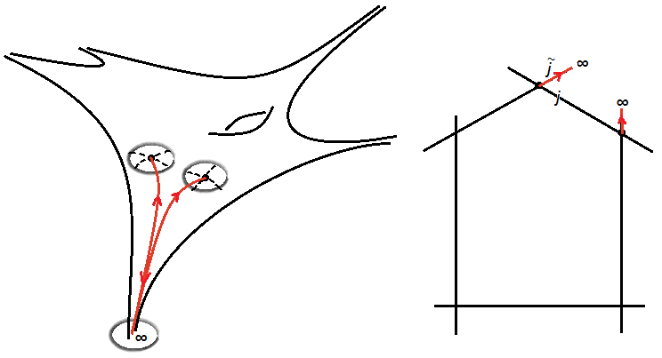
Figure 3.7: Transporting functions over the moduli

Explicitly, comparing the former local equation

$$\alpha^{\,p+1}+w_{p}\,\alpha^{\,p}+\cdots+w_{2}\,\alpha^{2}-h\,\alpha+w_{0}=0$$

to the latter local equation

$$(\alpha-p)\big{(}\alpha-(-1)^{\,p-1}\big{)}^{p}=0$$

we obtain the polynomial $w(h,\alpha)$ in Theorem 1.3 ($h$ becomes $(-1)^{\,p^{2}+1}+p^{2}\equiv 1\,~{}{\rm mod}~{}p$, consistent with [Katz-Mazur1985, 12.4.2]). This completes the proof of Theorem 1.3.

4 Proof of Theorems 1.8 and 1.9

Theorem 1.8 (i) follows from [Strickland1998, Theorem 1.1]. We show the remaining parts in two steps.

4.1 The total power operation formula and the Adem relations

To compute $\psi^{\,p}(h)$, we follow the recipe illustrated in [Zhu2015, Example 3.5] and generalize [ibid., proof of Proposition 6.4]. By (1.4) and (2.25), since

$$\begin{split}w(h,\alpha)=&~{}w_{p+1}\alpha^{\,p+1}+\cdots+w_{1}\alpha+w_{0}\\ =&~{}w_{p+1}\alpha^{\,p+1}+\cdots-h\,\alpha+\widetilde{\alpha}\,\alpha\end{split}$$

is zero in the target ring of $\psi^{\,p}$, we have

$$\hskip 14.22636pth=w_{p+1}\alpha^{\,p}+\cdots+w_{2}\,\alpha+\widetilde{\alpha}$$

where $w_{p+1}$, …, $w_{2}$ are constants, i.e., they do not involve $h$, as computed in Theorem 1.8 (i). Applying the Atkin-Lehner involution to this identity, we then obtain

$$\hskip-25.6073pt\psi^{\,p}(h)=\widetilde{h}=w_{p+1}\,\widetilde{\alpha}^{\,p}+\cdots+w_{2}\,\widetilde{\alpha}+\alpha$$

For $1\leq\tau\leq p$, we need only express each $\widetilde{\alpha}^{\tau}$ as a polynomial in $\alpha$ of degree at most $p$ with coefficients in $E^{0}$. The constant terms $d_{0,\tau}$ of these polynomials have been computed as $d_{\tau}$ in [Zhu2015, proof of Proposition 6.4]. The same method there applies to give the stated formulas for the higher coefficients $d_{i,\tau}$ with $1\leq i\leq p$. This completes the proof of Theorem 1.8.

To derive the Adem relations, we generalize [Zhu2014, proof of Proposition 3.6 (iv)] (cf. [Zhu2015, proof of Proposition 6.4]). In view of the relation $\alpha\cdot\widetilde{\alpha}=w_{0}$, we have

$$\begin{split}\psi^{\,p}\big{(}\psi^{\,p}(x)\big{)}=&~{}\psi^{\,p}\sum_{j=0}^{p}Q_{j}(x)\,\alpha^{\,j}\\ =&~{}\sum_{j=0}^{p}\psi^{\,p}\big{(}Q_{j}(x)\big{)}\,\psi^{\,p}(\alpha)^{\,j}\\ =&~{}\sum_{j=0}^{p}\Bigg{(}\sum_{i=0}^{p}Q_{i}Q_{j}(x)\,\alpha^{i}\Bigg{)}\widetilde{\alpha}^{\,j}\\ =&~{}\sum_{j=0}^{p}\Bigg{(}\sum_{i=0}^{j}w_{0}^{i}\,Q_{i}Q_{j}(x)\,\widetilde{\alpha}^{\,j-i}+\sum_{i=j+1}^{p}w_{0}^{\,j}\,Q_{i}Q_{j}(x)\,\alpha^{i-j}\Bigg{)}\\ =&~{}\sum_{k=0}^{p}\alpha^{k}\Bigg{(}\sum_{j=0}^{p}\sum_{i=0}^{j}w_{0}^{i}\,d_{k,\,j-i}\,Q_{i}Q_{j}(x)+\sum_{j=0}^{p-k}w_{0}^{\,j}\,Q_{k+j}Q_{j}(x)\Bigg{)}\end{split}$$

where $d_{k,0}=0$ if $k>0$ (and $d_{0,0}=1$ from before). Write the expression in last line above as $\sum_{k=0}^{p}\Psi_{k}(x)\,\alpha^{k}$. For $1\leq k\leq p$, the vanishing of each $\Psi_{k}$ then gives the stated relation for $Q_{k}Q_{0}$.

4.2 The commutation relations

To facilitate computations, let us make a change of variables $\beta\coloneqq\alpha+(-1)^{\,p}$. We then have

$$\begin{split}\psi^{\,p}(hx)=&~{}\psi^{\,p}(h)\,\psi^{\,p}(x)\\ =&~{}\sum_{i=0}^{p}Q_{i}(h)\,\alpha^{i}\,\sum_{j=0}^{p}Q_{j}(x)\,\alpha^{\,j}\\ =&~{}\sum_{m=0}^{2p}\!\Bigg{(}\!\!\sum_{\stackrel{{\scriptstyle\scriptstyle i+j=m}}{{0\,\leq\,i,\,j\,\leq\,p}}}\!\!Q_{i}(h)\,Q_{j}(x)\Bigg{)}\alpha^{m}\\ =&~{}\sum_{m=0}^{2p}\!\Bigg{(}\!\!\sum_{\stackrel{{\scriptstyle\scriptstyle i+j=m}}{{0\,\leq\,i,\,j\,\leq\,p}}}\!\!Q_{i}(h)\,Q_{j}(x)\Bigg{)}\!\big{(}\beta+(-1)^{\,p+1}\big{)}^{m}\\ =&~{}\sum_{m=0}^{2p}\!\Bigg{(}\!\!\sum_{\stackrel{{\scriptstyle\scriptstyle i+j=m}}{{0\,\leq\,i,\,j\,\leq\,p}}}\!\!Q_{i}(h)\,Q_{j}(x)\Bigg{)}\sum_{n=0}^{m}\!{m\choose n}\beta^{n}(-1)^{(p+1)(m-n)}\\ =&~{}\sum_{n=0}^{2p}e_{n}\,\beta^{n}\end{split}$$

where

$$e_{n}=\sum_{m=n}^{2p}(-1)^{(p+1)(m-n)}{m\choose n}\!\!\sum_{\stackrel{{\scriptstyle\scriptstyle i+j=m}}{{0\,\leq\,i,\,j\,\leq\,p}}}\!\!Q_{i}(h)\,Q_{j}(x)$$

Formulas for the terms $Q_{i}(h)$ above are given by Theorem 1.8 (ii). Note that $Q_{1}(h)$ includes a term of 1.

We now reduce $\psi^{\,p}(hx)$ above modulo $w(h,\alpha)$, by first rewriting the latter as a polynomial in $\beta$:

$$\begin{split}w(h,\alpha)=&~{}(\alpha-p)\big{(}\alpha+(-1)^{\,p}\big{)}^{p}-\big{(}h-p^{2}+(-1)^{\,p}\big{)}\alpha\\ =&~{}\big{(}\beta+(-1)^{\,p+1}-p\big{)}\beta^{\,p}-\big{(}h-p^{2}+(-1)^{\,p}\big{)}\big{(}\beta+(-1)^{\,p+1}\big{)}\\ =&~{}\beta^{\,p+1}+v_{p}\,\beta^{\,p}+v_{1}\,\beta+v_{0}\end{split}$$

where $v_{p}=(-1)^{\,p+1}-p$, $v_{1}=-\big{(}h-p^{2}+(-1)^{\,p}\big{)}$, and $v_{0}=(-1)^{\,p+1}v_{1}$. We then carry out a long division of $\psi^{\,p}(hx)$ by $w(h,\alpha)$ with respect to $\beta$ and obtain

$$\psi^{\,p}(hx)\equiv\sum_{j=0}^{p}\,f_{\,j}\,\beta^{\,j}\,~{}{\rm mod}~{}w(h,\alpha)$$

where

$$~{}~{}f_{\,j}=\left\{\hskip-2.84544pt\begin{array}[]{lll}\displaystyle e_{p}-v_{1}e_{2p}+v_{p}\sum_{m=0}^{p-1}(-1)^{m+1}e_{p+1+m}\,v_{p}^{m}&&\,j=p\\ \displaystyle e_{j}+v_{0}\sum_{m=0}^{p-j-1}(-1)^{m+1}e_{p+j+1+m}\,v_{p}^{m}+v_{1}\sum_{m=0}^{p-j}(-1)^{m+1}e_{p+j+m}\,v_{p}^{m}&&0<j<p\\ \displaystyle e_{0}+v_{0}\sum_{m=0}^{p-1}(-1)^{m+1}e_{p+1+m}\,v_{p}^{m}&&\,j=0\end{array}\right.$$

Thus we can rewrite

$$\begin{split}\psi^{\,p}(hx)=&~{}\sum_{j=0}^{p}\,f_{\,j}\,\big{(}\alpha+(-1)^{\,p}\big{)}^{\,j}\\ =&~{}\sum_{j=0}^{p}\,f_{\,j}\,\sum_{i=0}^{j}\!{\,j\,\choose i}\alpha^{i}\,(-1)^{\,p\,(\,j-i)}\\ =&~{}\sum_{i=0}^{p}\Bigg{[}\sum_{j=i}^{p}(-1)^{\,p\,(\,j-i)}{\,j\,\choose i}\,f_{\,j}\Bigg{]}\alpha^{i}\end{split}$$

On the other hand, $\psi^{\,p}(hx)=\sum_{i=0}^{p}Q_{i}(hx)\,\alpha^{i}$. Comparing this to the last expression for $\psi^{\,p}(hx)$ above, term by term, we obtain the commutation relations as stated. This completes the proof of Theorem 1.9.

. ​

References

Scott Ahlgren, The theta-operator and the divisors of modular forms on genus zero subgroups, Math. Res. Lett. 10 (2003), no. 6, 787–798. MR2024734

Matthew Ando, Isogenies of formal group laws and power operations in the cohomology theories $E_{n}$, Duke Math. J. 79 (1995), no. 2, 423–485. MR1344767

, Power operations in elliptic cohomology and representations of loop groups, Trans. Amer. Math. Soc. 352 (2000), no. 12, 5619–5666. MR1637129

Matthew Ando, Michael J. Hopkins, and Neil P. Strickland, The sigma orientation is an $H_{\infty}$ map, Amer. J. Math. 126 (2004), no. 2, 247–334. MR2045503

A. O. L. Atkin and J. Lehner, Hecke operators on $\Gamma_{0}(m)$, Math. Ann. 185 (1970), 134–160. MR0268123

Matthew H. Baker, Enrique González-Jiménez, Josep González, and Bjorn Poonen, Finiteness results for modular curves of genus at least 2, Amer. J. Math. 127 (2005), no. 6, 1325–1387. MR2183527

Mark Behrens and Charles Rezk, The Bousfield-Kuhn functor and topological André-Quillen cohomology, available at http://www3.nd.edu/~mbehren1/papers/BKTAQ8.pdf.

Jan H. Bruinier, Winfried Kohnen, and Ken Ono, The arithmetic of the values of modular functions and the divisors of modular forms, Compos. Math. 140 (2004), no. 3, 552–566. MR2041768

R. R. Bruner, J. P. May, J. E. McClure, and M. Steinberger, $H_{\infty}$ ring spectra and their applications, Lecture Notes in Mathematics, vol. 1176, Springer-Verlag, Berlin, 1986. MR836132

Kevin Buzzard, Analytic continuation of overconvergent eigenforms, J. Amer. Math. Soc. 16 (2003), no. 1, 29–55. MR1937198

Frank Calegari, Congruences between modular forms, available at http://swc.math.arizona.edu/aws/2013/2013CalegariLectureNotes.pdf.

D. Choi, On values of a modular form on $\Gamma_{0}(N)$, Acta Arith. 121 (2006), no. 4, 299–311. MR2224397

David A. Cox, Primes of the form $x^{2}+ny^{2}$, second ed., Pure and Applied Mathematics (Hoboken), John Wiley & Sons, Inc., Hoboken, NJ, 2013, Fermat, class field theory, and complex multiplication. MR3236783

P. Deligne and M. Rapoport, Les schémas de modules de courbes elliptiques, 143–316. Lecture Notes in Math., Vol. 349. MR0337993

Ethan S. Devinatz, Michael J. Hopkins, and Jeffrey H. Smith, Nilpotence and stable homotopy theory. I, Ann. of Math. (2) 128 (1988), no. 2, 207–241. MR960945

P. G. Goerss and M. J. Hopkins, Moduli spaces of commutative ring spectra, Structured ring spectra, London Math. Soc. Lecture Note Ser., vol. 315, Cambridge Univ. Press, Cambridge, 2004, pp. 151–200. MR2125040

Mike Hopkins, Complex oriented cohomology theories and the language of stacks, available at http://web.math.rochester.edu/people/faculty/doug/otherpapers/coctalos.pdf.

Michael J. Hopkins and Jeffrey H. Smith, Nilpotence and stable homotopy theory. II, Ann. of Math. (2) 148 (1998), no. 1, 1–49. MR1652975

Zhen Huan, Quasi-elliptic cohomology and its power operations, J. Homotopy Relat. Struct. 13 (2018), no. 4, 715–767. MR3870771

Nicholas M. Katz, $p$-adic properties of modular schemes and modular forms, Modular functions of one variable, III (Proc. Internat. Summer School, Univ. Antwerp, Antwerp, 1972), Springer, Berlin, 1973, pp. 69–190. Lecture Notes in Mathematics, Vol. 350. MR0447119

Nicholas M. Katz and Barry Mazur, Arithmetic moduli of elliptic curves, Annals of Mathematics Studies, vol. 108, Princeton University Press, Princeton, NJ, 1985. MR772569

Michel Lazard, Sur les groupes de Lie formels à un paramètre, Bull. Soc. Math. France 83 (1955), 251–274. MR0073925

J. Lubin, J.-P. Serre, and J. Tate, Elliptic curves and formal groups, available at http://www.ma.utexas.edu/users/voloch/lst.html.

Jonathan Lubin and John Tate, Formal moduli for one-parameter formal Lie groups, Bull. Soc. Math. France 94 (1966), 49–59. MR0238854

J. Lurie, A survey of elliptic cohomology, Algebraic topology, Abel Symp., vol. 4, Springer, Berlin, 2009, pp. 219–277. MR2597740

Mark Mahowald and Charles Rezk, Topological modular forms of level 3, Pure Appl. Math. Q. 5 (2009), no. 2, Special Issue: In honor of Friedrich Hirzebruch. Part 1, 853–872. MR2508904

Lennart Meier, Lifting the Hasse invariant mod 2, MathOverflow, http://mathoverflow.net/q/228497 (version: 2016-01-16).

J.S. Milne, Modular functions and modular forms, available at http://www.jmilne.org/math/CourseNotes/MF.pdf.

Bjorn Poonen, Supersingular elliptic curves and their “functorial” structure over ${\mathbb{F}}_{p^{2}}$, MathOverflow, http://mathoverflow.net/a/19013 (version: 2010-03-22).

Daniel Quillen, On the formal group laws of unoriented and complex cobordism theory, Bull. Amer. Math. Soc. 75 (1969), 1293–1298. MR0253350

Douglas C. Ravenel, Nilpotence and periodicity in stable homotopy theory, Annals of Mathematics Studies, vol. 128, Princeton University Press, Princeton, NJ, 1992, Appendix C by Jeff Smith. MR1192553

Charles Rezk, Power operations for Morava $E$-theory of height 2 at the prime 2. arXiv:0812.1320

, The congruence criterion for power operations in Morava $E$-theory, Homology, Homotopy Appl. 11 (2009), no. 2, 327–379. MR2591924

, Modular isogeny complexes, Algebr. Geom. Topol. 12 (2012), no. 3, 1373–1403. MR2966690

, Power operations in Morava $E$-theory: structure and calculations (Draft), available at http://www.math.uiuc.edu/~rezk/power-ops-ht-2.pdf.

, correspondence, 2013.

, correspondence, 2015.

, Rings of power operations for Morava E-theories are Koszul. arXiv:1204.4831

Stefan Schwede, Global homotopy theory, New Mathematical Monographs, vol. 34, Cambridge University Press, Cambridge, 2018. MR3838307

Joseph H. Silverman, The arithmetic of elliptic curves, second ed., Graduate Texts in Mathematics, vol. 106, Springer, Dordrecht, 2009. MR2514094

Neil P. Strickland, Finite subgroups of formal groups, J. Pure Appl. Algebra 121 (1997), no. 2, 161–208. MR1473889

, Morava $E$-theory of symmetric groups, Topology 37 (1998), no. 4, 757–779. MR1607736

J. T. Tate, $p$-divisible groups, Proc. Conf. Local Fields (Driebergen, 1966), Springer, Berlin, 1967, pp. 158–183. MR0231827

Jared Weinstein, Semistable models for modular curves of arbitrary level, Invent. Math. 205 (2016), no. 2, 459–526. MR3529120

Yifei Zhu, The power operation structure on Morava $E$-theory of height 2 at the prime 3, Algebr. Geom. Topol. 14 (2014), no. 2, 953–977. MR3160608

, The Hecke algebra action on Morava E-theory of height 2, available at https://yifeizhu.github.io/ho.pdf.

, Norm coherence for descent of level structures on formal deformations, available at https://yifeizhu.github.io/nc.pdf.

, Morava $E$-homology of Bousfield-Kuhn functors on odd-dimensional spheres, Proc. Amer. Math. Soc. 146 (2018), no. 1, 449–458. MR3723154