Uncertainty analysis and composite hypothesis under the likelihood paradigm
Abstract
The correct use and interpretation of models depends on several steps, two of which being the calibration by parameter estimation and the analysis of uncertainty. In the biological literature, these steps are seldom discussed together, but they can be seen as fitting pieces of the same puzzle. In particular, analytical procedures for uncertainty estimation may be masking a high degree of uncertainty coming from a model with a stable structure, but insufficient data.
Under a likelihoodist approach, the problem of uncertainty estimation is closely related to the problem of composite hypothesis. In this paper, we present a brief historical background on the statistical school of Likelihoodism, and examine the complex relations between the law of likelihood and the problem of composite hypothesis, together with the existing proposals for coping with it. Then, we propose a new integrative methodology for the uncertainty estimation of models using the information in the collected data. We argue that this methodology is intuitively appealing under a likelihood paradigm.
“In an ideal world, all data would come from well-designed experiments and would be sufficient to simultaneously estimate all parameters using rigorous statistical procedures. The world is not ideal. One must often combine estimates from different experiments, or supplement high-quality data (…) with uncertain data, or even assumptions (…). Think carefully about whether your conclusions may be artifacts of your assumptions or calculations, and document those assumptions and calculations so that your reader can ask the same question, and then carry on.”
(H. Caswell, Matrix Population Models)
1 Motivation
The use of mathematical and computational models is now widespread in several fields of the biological sciences. However, several applications of these models lack one or more steps that should be taken in order to correctly understand and interpret its results [Bart,, 1995]. Though seldom discussed together, five steps can be seen as fundamental in this process: verification, validation, calibration, uncertainty analysis and sensitivity analysis.
The two first steps are very tightly correlated, both in historical terms and in the common practice, so it’s common to refer to the set of validation and verification as “V & V”. We can think of verification as trying to ensure that the computer code is correctly implementing the desired model, while validation is trying to ensure that the theoretical model is capable of reproduce the actual phenomena of interest. Another way to see it is to think that validation is determining that the model is solving the right equations, while verification is determining that the model is solving the equations right [Meisner,, 2010].
The third step, calibration, consists in determining the right values for the input parameters of a model in order to enhance the correspondence between a model run and one observed situation. An appropriate calibration of the model is then essential for the model to be used in a predictive fashion [Meisner,, 2010].
The last steps consist in determining how much the variation of the input parameters is translated into the total variation of the results, which is called uncertainty analysis, and how much of the variation of the results can be ascribed to the variation of each individual parameter, which is called sensitivity analysis [Helton and Davis,, 2003; Helton et al.,, 2005]. These two have been extensively reviewed in another text ([Chalom and Prado,, 2012]), so we will just highlight the fact that these analyses, together with model calibration, strongly depend on previously and correctly executing the model verification and validation.
During the development and analysis of mathematical models in ecology, it is common to have completely separated procedures for calibration by parameter estimation (which we will call CPE) and sensitivity and uncertainty analyses (SUA) of a model. These steps are carried out in different sections of the research papers, discussed in different chapters of books (ie: [Caswell,, 1989]), and sometimes are even performed by different people. In matrix models for population projections, the results discussion is focused on a single combination of parameters, considered to be an optimum for the CPE, and the SUA is presented as a separate step, being secondary to the main results (see, for example, [Silva Matos et al.,, 1999]). We have no guarantees that even the statistical schools of though considered for both procedures will be coherent.
Moreover, the parameter set used in the model calibration may have few to no relation to parameters that have biological relevance. In the case of matrix models, the former may be parameters related to a time series, while the later might be the projection matrix entries. This way, the researcher responsible for the calibration may see the system as individual counts over time, while the researcher responsible for the uncertainty analyses will only be interested in the vital rates, which are real valued. When developed in such disparate worlds, the SUA will be unable to point out directions for the planning of new experiments or to single out which parameters should be targeted for more sampling effort.
This lack of integration between these fundamental steps for model analysis may have its roots in the development of the CPE and SUA theories. While the parameter estimation has always been seen as belonging to a statistical theory, the sensitivity of biological models was developed as an analytical tool, based on the linear expansion of functions around a privileged point. Depending on the nature of the experiments designed to measure vital rates, there may be a plethora of methods that might be used to determine the set of values that best represent the status of knowledge that we have about a given natural system - and these methods may stem from frequentist, Bayesian or likelihood-based approaches to the statistical theory. The analytical theory of SUA, on the other hand, is in great part due to the work of Hal Caswell [Caswell,, 1989], and proceeds by taking a model that is already optimally parametrized, and studying the first order derivatives of the model answer in relation to each input parameter. This formulation disregards completely the quantity and quality of collected data, except for their average, and sensitivity measures are taken exclusively over the variation of the model answer in response to infinitesimal changes. Thus, models that are parametrized by data with large uncertainties will not present larger sensitivity indexes than models parametrized by data with great precision. Increasing the sampling effort to gather data about the system will not affect the uncertainty values. We can conclude that the analytical formulation of the SUA, ultimately, gives information about the structure of the model, but is silent about the more embracing questions from the collection of field data to the formulation and execution of the model. This might lead to a false sense of confidence being placed on studies that present a stable matrix structure, leading to small sensitivity indexes, but use data with large uncertainties.
Other than this, questions about model validation are not usually addressed by literature in this field, but they are also intimately connected to the relevant questions about uncertainty. We can divide the uncertainty about a model in three main sources: structural uncertainty, parameter uncertainty and stochastic uncertainty (see [Marino et al.,, 2008] for a review about the latter two). While most of the SUA techniques are focused on the second component, the validation of a model may point out how much confidence we can have about whether one model (or a set of models) is adequate at representing the desired phenomena.
A stochastic formulation for a theory of global uncertainty and sensitivity analyses, as described in [Chalom and Prado,, 2012], and interpreted under the likelihood paradigm for statistics, is able to regard in the same way all of the uncertainty sources described above, generating a complete picture of our knowledge about a system. Although these formulations may converge for very simple systems, this is not the general case.
The main advantages of using a stochastic formulation are:
-
1.
The analytical procedures are local, thus responding only to what happens after infinitesimal perturbations, and depends on the model functions being “well-behaved” in the chosen neighborhood. The stochastic procedures are global and have no such limitation.
-
2.
Any stochastic approach allows for the information contained in the sample variability to be used to represent the uncertainty about the parameters.
-
3.
By accepting the Likelihood Principle, we know that all relevant information on the samples is contained in the associated likelihood function. This way, we can use the likelihood function alone to proceed in the analysis, while the analytical procedures at times will disregard information, and at times will lead to the false sensation of having more detailed information than the sample allows.
2 Historical background
The statistical use of likelihoods is very widespread, starting from Fisher’s definition on 1922, and spanning several schools of thought. On the one hand, the framework for Neyman-Pearson’s hypothesis testing is built upon it; on the other hand, it is a bridge between the a priori and a posteriori probabilities in Bayesian analysis. Starting on the decade of 1960, the use of likelihoods as a basis for statistical inference started to be more widely advocated as an alternative to both frequentism and Bayesianism. The 1965 book by Ian Hacking about the logic of inference and the 1972 book by A.W.F. Edwards on likelihoods can be seen as the starting points for this position to become an independent school of thought, sometimes called Likelihoodism. More recently, this position will be strongly supported by the works of Richard Royall and Elliott Sober.
The likelihoodist school of thought is based on the conjunction of the likelihood principle, as demonstrated by Allan Birnbaum, and the law of likelihood, as enunciated by Ian Hacking.
Birnbaum derived the likelihood principle in 1962, from two generally accepted principles111 This demonstration is controversial to this date. See [Mayo,, 2010] for a recent critique and [Gandenberger,, 2012] for a recent defense: the sufficiency principle and the conditionality principle. Informally, we can think about the two first affirming that “data that does not aggregate new information is irrelevant to the inference”, and “experiments that could have been realized but were not are irrelevant to the inference”. From this principles, Birnbaum deduces the likelihood principle, which can informally be stated as “experimental results which are possible but were not observed are irrelevant to the inference”. Or, in Birnbaum’s more formal terms:
“The likelihood principle: If and are any two experiments with the same parameter space, represented respectively by density functions and ; and if and are any respective outcomes determining the same likelihood function; then . That is, the evidential meaning of any outcome of any experiment is characterized fully by giving the likelihood function (which need be described only up to an arbitrary positive constant factor), without other reference to the structure of .” [Birnbaum,, 1962]
The law of likelihood was formulated by Hacking as:
“If hypothesis implies that the probability that a random variable takes the value is , while hypothesis implies that the probability is , then the observation is evidence supporting over if and only if , and the likelihood ratio, , measures the strength of that evidence.” [Hacking,, 1965]222Emphasis added
The divergence between the likelihood school and frequentist school is due to the later rejecting the likelihood principle (although it accepts the principles of sufficiency and conditionality). On the other hand, the Bayesian school generally disagrees with the Likelihoodists by the interpretation of the law of likelihood.
The likelihood school of thought can be seen as an intellectual heir to the Neyman-Pearson hypothesis testing framework, as its breaking point from Fisherian significance testing happens because of the logical necessity of comparing competing hypothesis. Fisher’s tests give a special privileged position to the so-called null hypothesis, which Neyman and Pearson will see as incomplete333 For a more complete and extremely didactic insight into their view, see the original paper from [Neyman and Pearson,, 1933]. The data gathered by one experiment may indicate a small or a large support for one given hypothesis, but this alone should not be considered as evidence in favor of this hypothesis before the other alternatives have been also scrutinized. In other words, the probability or improbability of a single hypothesis should not be used to conclude about its veracity. As the fictional detective Sherlock Holmes, by Sir Arthur Conan Doyle famously said, “How often have I said to you that when you have eliminated the impossible, whatever remains, however improbable, must be the truth?”.
However, while Neyman and Pearson will use the likelihood ratio from several hypothesis to guide the behavior of the scientist in accepting or rejecting hypothesis, Royall and Edwards will separate the concepts of (1) the degree of certainty that we have about one hypothesis; (2) the strength of evidence that some data confers to one hypothesis over the others and (3) the course of action that should be taken after examining such evidences. While Neyman and Pearson conflate the strength of evidence (2) with the course of action (3), and Bayesian analysis conflate the degree of certainty (1) with the strength of evidence (2), the proposers of Likelihoodism propose that the role of statistical inference is to provide only the strength of evidence [Royall,, 1997]. The degree of certainty and course of action should take into account a multiplicity of other factors, and should not be part of the inference. One of the greatest precursors of the statistical thought, Marquis Pierre-Simon de Laplace, had already foreshadowed this position with the problem of the number of judges necessary to convict or acquit a prisoner: this decision, to Laplace, needs to take into account not only the probability of convicting an innocent of acquitting a guilty prisoner, but also whether the punishment will be a fine or the death sentence[Laplace,, 1814].
Moreover, by dissociating the strength of evidence from the decision making, Royall and Edwards are asking the scientist to reveal the untransformed likelihood ratios derived from its data, instead of transforming it into p-values or a posterioris, so that her peers are able to assess clearly what is the presented evidence. By retaking the scientist role as a subjective decision maker, this proposition converges to Fisher’s, who criticized Neyman-Pearson’s plan as being useful for industrial processing, but useless to the scientific community. The likelihoodist proposal thus echoes the words of Fisher, and also the words of the Bayesian probabilist I. J. Good:
“We have the duty of formulating, of summarizing, and of communicating our conclusions, in intelligible form, in recognition of the right of other free minds to utilize them in making their own decisions.” [Fisher,, 1955]
“If a Bayesian is a subjectivist, he will know that the initial probability density varies from person to person and so he will see the value of graphing the likelihood function for communication.” [Good,, 1976]
However, there is a very important difference between the Bayesian and the Likelihoodist paradigms: the a posteriori probabilities, constructed by the multiplication of the likelihood by an a priori probability under the Bayesian school, is a absolute quantity. It is thus possible to refer to the a posteriori probability of event , or the a posteriori probability of an event . In contrast, the Likelihoodist approach will see in the likelihood ratio the end point for the statistical analysis. This is why the law of likelihood is expressed over evidence supporting over : because the likelihoodist approach does not allow for the transformation of the relational support of over to be translated into non-relational quantities of support for each hypothesis444See the text by [Fitelson,, 2007] for more details on this matter, including Carnap’s classification of confirmation.
3 The challenge for uncertainty estimation
From this section, we will consider problems where represent a vector of data obtained independently from one or more experiments from a vector-valued random variable , such that . The parameter vector is unknown and may assume values in . We will refer to the likelihood of given the observed data as . The likelihood ratio over the same data set can be abbreviated as .
In order to perform an uncertainty analyses for a mathematical model under the likelihood paradigm, the general question that we would like to answer can be written as: “how much support does the collected data provide for the concurrent hypothesis over the model results?”. For example, in a population growth model, the question may become “how much support the collected data provide for the hypothesis that the population is growing at the rate of 1 individual per year, versus the hypothesis that it is stable ?”555As we will see, the question can become more general, such as “how much support the collected data provide for the hypothesis that the population is growing or stable versus the hypothesis that is declining?”
This question, formulated over the parameters of a probability distribution, should be answered by means of the likelihood function. It can be demonstrated that one-to-one functions over the parameters preserve the likelihood function, such that if is the likelihood of and is given by a one-to-one function , the likelihood of is given by [Edwards,, 1972].
However, the application of a mathematical model is analogous to the application of a generic function, and the reasoning above does not hold for arbitrary many-to-one functions. Thus, defining a methodology for uncertainty analyses of arbitrary models is closely related to the problem of composite statistical hypotheses. However, the law of likelihood is expressed in terms of simple statistical hypothesis, and there is no way of combining these values to form the “likelihood of a composite hypothesis”. As Edwards writes:
“No special meaning attaches to any part of the area under a likelihood curve, or to the sum of the likelihoods of two or more hypotheses (…). Although the likelihood function, and hence the curve, has the mathematical form of a [known] distribution, it does not represent a statistical distribution in any sense.” [Edwards,, 1972]
How can we work with composite hypothesis then? The traditional answer from the proposers of Likelihoodism is that we don’t. Edwards puts off composite hypothesis as “uninteresting to science”, while Royall sees this restriction to simple hypothesis as an advantage, not a limitation, to the likelihood approach. However, this is necessary if we want to derive an uncertainty estimation for model results. Here, we will present three paths that may be pursued for this end:
-
1.
Formulate a new law of likelihood, which can be applied for composite hypothesis;
-
2.
Present a methodology based on a logical extension of the law of likelihood;
-
3.
Address the issue using a model similar to the one applied for nuisance parameters.
Proposal 1 is based on the axiomatic formulation of a generalized law of likelihood (GLL) that is compatible with the law of likelihood (LL) for simple hypothesis for simple hypothesis, but able to extend its domain for composite hypothesis. And proposal 2 is based on the use of a weaker definition of statistical evidence, based on a weak law of likelihood (WLL). We will review some existing results related to these proposals in the following sections.
Proposal 3 is based on methods such as profiled likelihood, which are ad hoc methods widely used to reduce the study of multiparametric statistical models to visualizing one parameter at a time. A typical use for these methods is exemplified by the problem of fitting a normal distribution over some data. While, strictly, the comparable hypothesis must be given by pairs , representing one value for the mean and on for the variance of the distribution, it is possible to compare the approximate support for different values for the mean, while leaving the variance free to assume any viable value - thus treating the composite hypothesis . We will get back to this proposal in section 6.
4 GLL: A general law of likelihood
The most straightforward way to pursue a general law of likelihood is by considering the maximum666 Or more precisely, the supremum, as the set of likelihoods does not need to have a maximum of the likelihoods of the simple hypothesis as the likelihood of the composite hypothesis. This is precisely the path followed by Zhang, [2009]; Zhang and Zhang, [2013] and Bickel, [2010]. We will follow the more didactic approach by Zhang. Let us consider two hypothesis, versus . Now we postulate the following two axioms777The notation was sightly altered for coherency with the other sections:
Axiom 4.1.
If , then the observation is evidence supporting over .
Axiom 4.2.
If is evidence supporting over and implies , then is evidence supporting over .
The first axiom ensures that if the images of and are disjoint intervals, or in other words, if every simple hypothesis that implies is supported over every simple hypothesis that implies , then is supported over . There seem to be no reason to reject this axiom, other than a predisposition to ignore composite hypothesis. The second axiom is used to ensure a form of logical coherence. It is important to stress that this coherence axiom is not used to suppose that the logic structure of the hypothesis is somehow preserved in the likelihood function. In particular, if implies , the axiom 4.2 does not warrant the assertion that is better supported than .
From these axioms, we can derive the following general law of likelihood (GLL):
Theorem.
(GLL) “If , then there is evidence supporting over .” [Zhang,, 2009]
Proof.
The use of a “generalized likelihood ratio” given by seems natural to quantify the strength of evidence, just as the likelihood ratio is used to quantify the strength of evidence under the law of likelihood (LL). It is trivial to see that the GLL is compatible with LL in the case of simple hypothesis, and with some particular cases proposed by [Royall,, 1997]. However, it is striking to see that this formulation of the GLL allows for an absolute degree of hypothesis confirmations. One hypothesis can be absolutely supported if , where c represents the complimentary set. That is equivalent to . This absolute likelihood will always be zero for simple hypothesis concerning real values parameters, but this does not happen then is finite.
On the other hand, accepting the generalized likelihood ratio makes it impossible for a researcher to combine evidence from multiple data sources, as the generalized likelihood is not a multiplicative quantity. So, the greatest problem here is to find a generalization that allows for a measure of strength of evidence that can be combined across experiments.
5 WLL: A weak law of likelihood
A more general way of expressing statistical support is given by
- WLL
-
“Evidence favors hypothesis over hypothesis if and .” [Fitelson,, 2007]
Evidently, LL WLL. However, WLL is also implied by most modern Bayesian proponents. Given a confirmation measure , the Bayesian equivalent for the LL is:
-
“Evidence favors hypothesis over hypothesis according to measure if and only if .” [Fitelson,, 2007]
There are three main formats for the confirmation measures:
- Difference
-
- Ratio
-
- Likelihood ratio
-
It is important to remember that the Bayesian confirmation given by has a non-relational nature, and the relation confirmation is constructed by comparing two of those measures. Likelihoodists will see in the LL a primitive relational relation. While the construction of the non-relational confirmation measures depends on the specification of a prioris, the WLL makes no such assumptions, using only catch-all probabilities (the terms). One theory based on the WLL without invoking a prioris could be used as a base to an intermediate inference school of thought, one that is not dependent on the specification of a prioris, but without the arbitrary restriction on the use of composite hypothesis.
6 PLUE: a proposal for likelihood profiling
In this section, we will describe how the profiling techniques for likelihood functions can be seen as a foundation for a methodology of uncertainty estimation for mathematical models. We reason that this methodology is intuitively appealing under a likelihood paradigm; and we will refer to it as PLUE - Profiled Likelihood Uncertainty Estimation.
6.1 Intuition
Suppose that we have one mathematical model, for example a structured population growth model like those exemplified in [Chalom and Prado,, 2012], and one data set from which we can estimate the vital rates of the population, such as survival, growth and fertility rates.
With this data in hands, we would like to ask the following questions:
“What is the support given by the data to the affirmation that the population is stable versus that it is declining? What is the support given by the data to the affirmation that the population will become extinct in up to 10 years versus more than 10 years?”
These questions cannot be answered under a strict Likelihoodist point of view, as they refer to composite hypothesis over the parameters. However, we can take the maximum likelihood point as privileged and restrict the question to the form:
“What is the support given by the data to point of maximum likelihood versus any point in which the population growth is negative?”
Schematically, we can see in figure 1 that we are comparing the likelihood at the global maximum () with the maximum value attained at a distinct region (). This kind of question is now comparing one simple hypothesis, corresponding to the maximum likelihood, with a composite hypothesis. This kind of comparison avoids the problems and quirks that afflict the general laws of likelihood due to the superposition of likelihood intervals. In terms of the Zhang axioms (see section 4), we are accepting a weak form of the first, but not the second.
This reasoning can be extended to the following:
“Which are the points in the parameter space for which the support given by the data versus the point of maximum likelihood is greater than a certain threshold ?”
By asking the same question for different values of , we are effectively profiling the likelihood surface for the parameter space. In this point, we need to remember that profiling methods for likelihood are used in inference since the decade of 1970 to reduce the dimensionality of parameters spaces, in particular in the form of elimination of “nuisance parameters”. Even if the status of this procedures is not fully understood under the likelihood paradigm (see for example [Kalbfleisch and Sprott,, 1970] for the relation between nuisance parameters and fiducial inference), these methods are generally accepted as a valid procedure for exploratory analysis.
We have already discussed the typical example of fitting a normal distribution to a data set. In this example, the likelihood is defined for pairs , but it is usual to make affirmations about the average of the distribution, without referring to . However, this is equivalent to consider the model , that is, a model that projects the bi-dimensional space formed by and into an unidimensional space. Our proposal is merely to use this same reasoning for general non-invertible functions. Even if this is nothing new under the optics of the likelihood profiling, this is the first time that this methodology is proposed in the literature of uncertainty analyses, to the best of our knowledge.

6.2 Method
- Definitions
-
Consider first a mathematical model of interest. We will call this the “biological model”888 But it could be a physical model, hydrological model, geochemical model, etc. to differentiate between this and the statistical model presented below. We will consider the simple case of a scalar response for a model with a vector input : .
Let’s represent by the set of data collected in field or laboratory experiments. If we have parameters and observations, is a table with columns and rows.
Now formulate different models to explain your data (ex: constant or grouped fertility, constant or decreasing growth rate, models with 4 or 5 size classes, etc.). These will be the statistical models. Write the likelihood function for each model, find the best set of parameters that fits your data and determine the value of AIC for each statistical model (see for example [Burnham and Anderson,, 2002] for details in this step).
- Sampling
-
Take the model with the best AIC, and use a Monte Carlo sampling to generate a large number of samples with density proportional to (for example, use the Metropolis algorithm [Tierney,, 1994]). We will call this sample . To each element in (taken from ), we have associated the value of , the likelihood of this sample, and we take , the result of the biological model over this sample. Normalize to have the minimum log-likelihood in .
- Aggregation
-
Now we take the model results and associated likelihoods , and create an upper profile in the following manner: for each increment , find the largest value in such that . Note down this value as , and repeat for a larger value of .
Proceed in an analogous fashion to build the lower likelihood profile. Both profiles, taken together, can be used to investigate the plausibility regions of under .
7 Case study: a minimal model for population growth
Here, we will study a structured population model that be considered minimal: the life stages are non-reproducing juveniles and reproductive adults. This example is presented by [Caswell,, 2008] as a simple example of the analytical sensitivity analysis. The model is described by the following matrix:
| (1) |
Here, is the probability of juvenile survival, is the probability of adult survival, is the maturation probability and is the adult fertility. We will represent by the largest eigenvalue of this matrix, and consider this as the model response.
To simplify some calculations, let’s presume that the survival rate does not depend on the life stage (). We will also suppose that it is possible to unequivocally mark the juveniles that were born in the last time interval, and which passed through the maturation process to become adults in the last time interval. The model becomes:
| (2) |
For large animals with one offspring for reproductive seasons, such as whales, can be modeled as the proportion of adults that generate offspring. The parameter is modeled as the proportion of individuals that survive from one time interval to another, and as the proportion of juveniles that maturate from one time interval to another. This way, all of the three parameters can be modeled as binomial distributions with unknown probabilities and number of trials given by , the number of juveniles, , the number of adults, and , the total population size:
| (3) | ||||
| (4) | ||||
| (5) |
We will also assume that the parameters are independent, to arrive at the likelihood functions graphed in 2 (mathematical details are presented in section 7.1).
We will examine a numerical example with the initial population having 10 juveniles and15 adults. The population size is very small, which is important to highlight the difference between the analytical and stochastic approaches. After one time step, we can see 3 recent adults, 2 born juveniles and 23 total survivors. It’s easy to see from the figure 2 that the best estimate for this parameters is given by 0.92, 0.13 and 0.3. Also, the corresponding value for is 1.02.
The likelihood functions for each parameter were used to generate 50000 samples using Metropolis algorithm, from which we derive an empirical distribution for , which is proportional to likelihood of the parameters. This distribution, together with the likelihood values associated with each input, was used to construct a likelihood profile for the model result. The minimum likelihood for is attained in 1.02.
Figures 4 and 5 show preliminary results of the application of sensitivity techniques (such as described in [Chalom and Prado,, 2012]) to the generated samples. It is important to highlight that this analyses have been carried out in a neighborhood of the maximum likelihood point that is not infinitesimal, nor arbitrary, which would be the case in analytical and other stochastic methods.


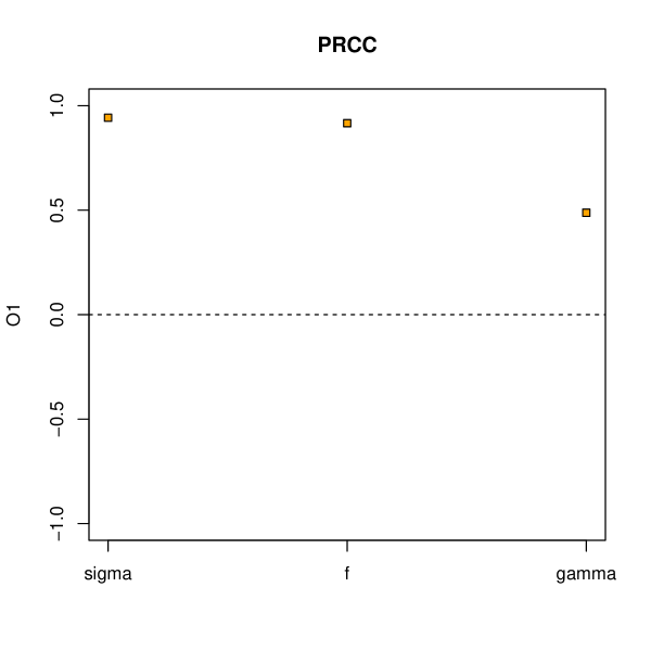
The analysis shown indicates that the estimated value of is very unreliable, presenting a very open profile. It is important to notice that this happens due to the small sample size. If we consider a sample in which all the observations are 3 times larger, but keeping all the proportions, the analysis results in a more closed profile (fig. 6).

7.1 Mathematical details
In this section, we will detail some mathematical points left out in the example above.
For a given observed number of juveniles that have undergone maturation, becoming adults in the last time interval, , we can write the log-likelihood function for as:
| (6) |
In the same way, the log-likelihood for is related to the number of juveniles that were born in the last time interval, , by the expression:
| (7) |
And last, the log-likelihood function is given over the number of surviving individuals (or the total population minus ):
| (8) |
With the strong assumption that the three variables are independent, we can write and in order to arrive at the more economical notation999 It is important to remember that is not the number of juveniles, and so on. for the likelihood function over the entire parameter vector :
| (9) |
The result of the model is , the largest eigenvalue in . For 2x2 matrices, this is given simply by:
| (10) |
| (11) |
7.2 R code for performing the analyses
In this section, we will present the R code used to generate the analyses and graphs presented above. This can be seen as a tutorial in the usage of the computational tools provided in the “pse” package. You should have installed R 101010This tutorial was written and tested with R version 3.0.1, but it should work with newer versions along with an interface and text editor of your liking, and the package “pse” (available on http://cran.r-project.org/web/packages/pse).
7.2.1 Biological and statistical models
First, we should define our interest model. We will refer to this model as the biological model111111 Because the models of interest in my research are biological. It can also be a physical model, geochemical model, etc. to distinguish this from the statistical model we will be using to estimate likelihoods. This model must be formulated as an R function that receives a data.frame, in which every column represent a different parameter, and every line represents a different combination of values for those parameters. The function must return an array with the same number of elements as there were lines in the original data frame, and each entry in the array should correspond to the result of running the model with the corresponding parameter combination. For example, it can be this121212See the preceding sections for the interpretation of the model, including parameters and results:
> tr <- function (A) return(A[1,1]+A[2,2])> A.to.lambda <- function(A)+ 1/2*(tr(A) + sqrt((tr(A)^2 - 4*det(A))))> getlambda = function (sigma, f, gamma) {+ A.to.lambda (matrix(c(sigma*(1-gamma), f,+ sigma*gamma, sigma),+ ncol=2, byrow=TRUE) )+ }> getlambda = Vectorize(getlambda)> model <- function(x) getlambda(x[,1], x[,2], x[,3])
Following the definition of the model, we should define the likelihood function for our parameters. To do this, we can formulate and test several statistical models. In order to fit competing models to the data and select the best of them, we recommend using the R package bbmle. Then, the best model should be written as a function receiving a numeric vector representing one realization of the parameter vector and returning the positive log-likelihood of that vector.
For example, the best model may be that the parameters , and are all independent from each other, coming from the specified binomial distributions:
> # Initial population: juveniles, adults, total> n <- c(10, 15); n.t <- sum(n)> # Observed quantities: matured, born, survival> obs <- c(3, 2, 23)> # Best guess for the parameters> sigma <- obs[3]/n.t> f <- obs[2]/n[2]> gamma <- obs[1]/n[1]> lambda <- getlambda(sigma, f, gamma)
The likelihood function, in this case, should be:
> # NOTE: LL function uses GLOBAL obs and n!!!> LL <- function (x)+ {+ t <- dbinom(obs[3], n.t, as.numeric(x[1]), log=TRUE) ++ dbinom(obs[2], n[2], as.numeric(x[2]), log=TRUE) ++ dbinom(obs[1], n[1], as.numeric(x[3]), log=TRUE)+ if (is.nan(t)) return (-Inf);+ return(t);+ }
Please note that this function uses the global variable obs, and that it return minus infinity instead of not-a-number in cases where the likelihood is not properly defined. This can happen, for instance, if any of the values of x is negative.
7.2.2 Profiling: sampling and aggregating the results
After carefully constructing the model of interest and the likelihood function, as described in the previous section, performing the PLUE analysis is simply a matter of calling the PLUE function. This function performs three steps. First, it performs a Monte Carlo sampling of the likelihood function in order to generate a large sample from the likelihood distribution. Then, the biological model is applied to this sample, and finally the model results are combined by means of profiling the likelihood function associated with each data point.
The pse package implements a simple Metropolis sampling function that can be used by setting method=‘internal’ in the PLUE function call. For more elaborate sampling schemes, and more control over the process, we recommend using method=‘mcmc’, which uses the mcmc R package.
> library(pse)> factors = c("sigma", "f", "gamma")> N = 50000> # we set the random seed to ensure reproducibility:> set.seed(42)> # The starting point for the Monte Carlo sampling> start = c(sigma, f, gamma)> plue <- PLUE(model, factors, N, LL, start,+ method="mcmc", opts=list(blen=10), nboot=50)
In order to see the profiled likelihood of the model result, simply run:
> plot(plue, xlim=c(0.6, 1.3))
Notice that additional parameters may be specified for the underlying plotting function, such as xlim, ylab or main. Additional plots may be seen by using the plotscatter and plotprcc functions:
> # Sensitivity analyses over lambda> plotscatter(plue)> plotprcc(plue)
The interpretation of these graphs is analogous to those generated by the Latin Hypercube Sampling, as described in [Chalom and Prado,, 2012]. However, it is important to notice that, instead of the arbitrary region of the parameter space that is sampled in the LHS scheme, the plots presented in this document are representing a discretization of the likelihood surfaces of the parameters, thus incorporating all the information about the data collected.
Acknowledgments
This work was supported by a CAPES scholarship.
References
- Bart, [1995] Bart, J. (1995). Acceptance criteria for using indivual-based models to make management decisions. Ecological applications, 5(2):411–420.
- Bickel, [2010] Bickel, D. (2010). The strength of statistical evidence for composite hypotheses: Inference to the best explanation. COBRA Preprint Series.
- Birnbaum, [1962] Birnbaum, A. (1962). On the foundations of statistical inference. Journal of the American Statistical Association, 57(298):269–326.
- Burnham and Anderson, [2002] Burnham, K. and Anderson, D. (2002). Model Selection and Multimodel Inference: A Practical Information-Theoretic Approach. Springer.
- Caswell, [1989] Caswell, H. (1989). Matrix population models. John Wiley & Sons.
- Caswell, [2008] Caswell, H. (2008). Perturbation analysis of nonlinear matrix population models. Demographic Research, 18:59–116.
- Chalom and Prado, [2012] Chalom, A. and Prado, P. (2012). Parameter space exploration of ecological models. arXiv:1210.6278 [q-bio.QM].
- Edwards, [1972] Edwards, A. (1972). Likelihood. Cambridge University Press, Cambridge.
- Fisher, [1955] Fisher, R. (1955). Statistical methods and scientific induction. Philosophical Transactions of the Royal Society of London. Series B, 17:69–78.
- Fitelson, [2007] Fitelson, B. (2007). Likelihoodism, Bayesianism, and relational confirmation. Synthese, 156(3):473–489.
- Gandenberger, [2012] Gandenberger, G. (2012). A new proof of the likelihood principle. British Journal for the Philosophy of Science.
- Good, [1976] Good, I. (1976). The Bayesian influence, or how to sweep subjectivism under the carpet. In Harper, W. and Hooker, C., editors, Foundations of probability theory, statistical inference, and statistical theories of science, page 0. Reidel.
- Hacking, [1965] Hacking, I. (1965). Logic of statistical inference. Cambridge university press, New York.
- Helton et al., [2005] Helton, J., Davis, F., and Johnson, J. (2005). A comparison of uncertainty and sensivity analysis results obtained with random and latin hypercube sampling. Reliability Engineering and System Safety, 89:304–330.
- Helton and Davis, [2003] Helton, J. and Davis, J. (2003). Latin hypercube sampling and the propagation of uncertainty in analyses of complex systems. Reliability Engineering and System Safety, 81:23–69.
- Kalbfleisch and Sprott, [1970] Kalbfleisch, J. D. and Sprott, D. A. (1970). Application of likelihood methods to models involving large numbers of parameters. Journal of the Royal Statistical Society. Series B (Methodological), pages 175–208.
- Laplace, [1814] Laplace, P. (1814). Essai philosophique sur les probabilités. Bachelier, imprimeur-libraire, Paris.
- Marino et al., [2008] Marino, S., Hogue, I., Ray, C., and Kirschner, D. (2008). A methodology for performing global uncertainty and sensivity analysis in systems biology. Journal of Theoretical Biology, 254:178–196.
- Mayo, [2010] Mayo, D. (2010). An error in the argument from conditionality and sufficiency to the likelihood principle. In Mayo, D. and Spanos, A., editors, Error and Inference: Recent Exchanges on Experimental Reasoning, Reliability and the Objectivity and Rationality of Science, pages 305–314. Cambridge University Press.
- Meisner, [2010] Meisner, R. (2010). Advanced Simulation and Computing Program Plan FY11. Technical report, Office of Advanced Simulation and Computing, NNSA Defense Programs. NA-ASC-122R-10.
- Neyman and Pearson, [1933] Neyman, J. and Pearson, E. (1933). On the problem of the most efficient tests of statistical hypotheses. Philosophical Transactions of the Royal Society of London. Series A, 231:289–337.
- Royall, [1997] Royall, R. (1997). Statistical Evidence: A Likelihood Paradigm. Chapman and Hall, London.
- Silva Matos et al., [1999] Silva Matos, D., Freckleton, R., and Watkinson, A. (1999). The role of density dependence in the population dynamics of a tropical palm. Ecology, 80(8):2635–2650.
- Tierney, [1994] Tierney, L. (1994). Markov chains for exploring posterior distributions (with discussion). Annals of Statistics, pages 1701–1762.
- Zhang, [2009] Zhang, Z. (2009). A law of likelihood for composite hypotheses. arXiv:0901.0463 [math.ST].
- Zhang and Zhang, [2013] Zhang, Z. and Zhang, B. (2013). A likelihood paradigm for clinical trials. Journal of Statistical Theory and Practice, 7(2):157–177.