Dimensional Crossover in a Spin-imbalanced Fermi gas
Abstract
We model the one-dimension (1D) to three-dimension (3D) crossover in a cylindrically trapped Fermi gas with attractive interactions and spin-imbalance. We calculate the mean-field phase diagram, and study the relative stability of exotic superfluid phases as a function of interaction strength and temperature. For weak interactions and low density, we find 1D-like behavior, which repeats as a function of the chemical potential as new channels open. For strong interactions, mixing of single-particle levels gives 3D-like behavior at all densities. Furthermore, we map the system to an effective 1D model, finding significant density dependence of the effective 1D scattering length.
pacs:
67.85.Lm, 74.20.-z, 03.75.Hh, 71.10.PmI Introduction
Spin-imbalanced Fermi gases are predicted to display an array of exotic superconducting phases, where the order parameter has non-trivial structure 3DsmallFFLO+BP1indeepBEC+detection+noncond ; 3DsmallFFLO+BPintro+BP1indeepBEC+detection ; 3DsmallFFLO+BPintro+BP1indeepBEC ; 3DsmallFFLO+BP1indeepBEC+noncond ; 3DsmallFFLO+BP1indeepBEC ; 3DsmallFFLO ; 3DsmallFFLO+Hartree+regularizationLDA ; 3D+ASLDA ; 1DrichphasesMF ; 1DrichphasesMF+mapping+1Dphasediagram+exactvsMF ; 1Drichphases+1Dexperiment+1Dphasediagram ; 1Drichphases+1Dphasediagram+mapping ; 1Drichphases+1Dphasediagram ; 1Drichphases ; 1Drichphases+quasi1Dpromising ; 1drichphases+detection ; FR+ ; DFS+detection ; mixedphase+detection ; BP+display ; detection+ ; noncond+ ; display ; liquidcrystal . Mean-field theories predict that these states occupy a very small fraction of the phase diagram in 3D, but are ubiquitous in 1D 3DsmallFFLO+BP1indeepBEC+detection+noncond ; 3DsmallFFLO+BPintro+BP1indeepBEC+detection ; 3DsmallFFLO+BPintro+BP1indeepBEC ; 3DsmallFFLO+BP1indeepBEC+noncond ; 3DsmallFFLO+BP1indeepBEC+noncond ; 3DsmallFFLO+BP1indeepBEC ; 3DsmallFFLO ; 3DsmallFFLO+Hartree+regularizationLDA ; 1DrichphasesMF ; 1DrichphasesMF+mapping+1Dphasediagram+exactvsMF , with the caveat that quantum fluctuations prevent long-range order in 1D longrangeorder . Indeed, cold-atom experiments in 3D 3dexperiments have found no sign of the exotic Fulde-Ferrell-Larkin-Ovchinnikov (FFLO) phase FFLO , while experiments on 1D tubes 1Drichphases+1Dexperiment+1Dphasediagram found thermodynamic evidence for a fluctuating version 1Drichphases+1Dphasediagram+mapping ; 1Drichphases+1Dphasediagram ; 1Drichphases ; 1Drichphases+quasi1Dpromising ; 1drichphases+detection of FFLO, but were unable to measure the order parameter. One avenue for directly observing these exotic superfluid states is to use highly anisotropic quasi-1D geometries where they should be robust 1Drichphases+quasi1Dpromising ; quasi1Dpromising+quasi1Dsingleband+mapping ; quasi1Dpromising+detection ; quasi1Dfinitesize+BP ; quasi1Dfinitesize ; quasi1Dpromising ; quasi1Dpromising+quasi1Dsingleband+detection ; quasi1Dpromising+bolechFFLOdetection ; quasi1Dpromising+quasi1Dsingleband ; quasi1Dpromising+quasi1Dfinitesize+ASLDA . Here we solve the Bogoliubov-de-Gennes (BdG) equations in such a geometry. We find large regions of the phase diagram in which the FFLO finite-momentum-pairing state is stable. We also find a stable breached-pair (BP) state where pairs coexist with a Fermi surface 3DsmallFFLO+BPintro+BP1indeepBEC+detection ; 3DsmallFFLO+BPintro+BP1indeepBEC ; BPintro+detection ; BPintro ; BPintro+interiorgap ; BPintro+quarkmatter+BP1indeepBEC+topology . Our analysis provides a much needed narrative for thinking about the 1D-3D crossover, going beyond the existing single-band models quasi1Dpromising+quasi1Dsingleband+mapping ; quasi1Dsingleband+mapping ; quasi1Dsingleband ; quasi1Dpromising+quasi1Dsingleband+detection ; quasi1Dpromising+quasi1Dsingleband and studies of finite systems quasi1Dfinitesize+BP ; quasi1Dfinitesize ; quasi1Dpromising+quasi1Dfinitesize+ASLDA . While we focus on cold atoms, these considerations are also relevant to nuclear, astrophysical condmatter+quarkmatter ; BPintro+quarkmatter+BP1indeepBEC+topology ; quarkmatter , and condensed-matter systems condmatter+quarkmatter ; condmatter+FFLOdetected ; condmatter . Evidence of the FFLO phase has recently been found in a quasi-2D superconductor condmatter+FFLOdetected , and there are ongoing attempts to see related physics in 2D atomic systems 2DatomsFFLO .
We consider a harmonic oscillator potential of frequency which confines the motion of the atoms in the - plane. The atoms are free to move in the direction, have mass , and interact via -wave collisions, characterized by a scattering length (tuned via a Feshbach resonance FR+ ; FRreview ). We consider the “Bardeen-Cooper-Schrieffer (BCS) side” of resonance where , and calculate the mean-field phase diagram in the - plane, where and denote respectively the average chemical potential and the chemical potential difference of the two spins. Prior work on this model has examined the low-density (small ) limit, where the transverse motion of the atoms are confined to the lowest oscillator level 1DrichphasesMF+mapping+1Dphasediagram+exactvsMF ; 1Drichphases+1Dexperiment+1Dphasediagram ; 1Drichphases+1Dphasediagram+mapping ; quasi1Dpromising+quasi1Dsingleband+mapping ; quasi1Dsingleband+mapping , and the system maps onto an effective 1D model mapping . Conversely, when is large, the atoms can access many energy levels of the trap, and the system is locally three-dimensional. Here we investigate the crossover between these regimes.
The exact 1D phase diagram contains three phases which are fluctuating analogs of the BCS superfluid, the FFLO state, and a fully polarized (FP) gas 1DrichphasesMF+mapping+1Dphasediagram+exactvsMF ; 1Drichphases+1Dexperiment+1Dphasediagram ; 1Drichphases+1Dphasediagram+mapping ; 1Drichphases+1Dphasediagram . Since interaction effects in 1D are stronger at low densities, pairs are more stable at smaller , and the slope of the line separating the BCS and FFLO phases has a negative slope. The analogous phase boundary in 3D has a positive slope, providing a convenient distinction between 1D-like and 3D-like behavior. In 3D there is also a partially polarized Normal (N) state 3DsmallFFLO+BPintro+BP1indeepBEC+detection ; 3DsmallFFLO+BPintro+BP1indeepBEC .
For weak interactions and , we find 1D-like behavior, in that . The critical field jumps whenever a new channel opens (near ), but after this jump we again find (Fig. 1a). Once many channels are occupied we find 3D-like behavior with . Each 1D-like interval hosts a large FFLO region. In the 3D regime, these regions merge to form a single domain. As interactions are increased, the crossover to 3D-like behavior moves to smaller (Fig. 2a). For very strong interactions near unitarity (), the harmonic oscillator levels are strongly mixed, and we always find . (Fig. 2b). Regardless, we find that the FFLO phase occupies much of the phase diagram for all interaction strengths. Moreover, at sufficiently strong interactions, we find a BP region, nestled between the BCS and the FFLO phases. Such a (zero-temperature) BP phase is stable in 3D only for negative in the deep Bose-Einstein condensate (BEC) side of resonance () 3DsmallFFLO+BP1indeepBEC+detection+noncond ; 3DsmallFFLO+BPintro+BP1indeepBEC+detection ; 3DsmallFFLO+BPintro+BP1indeepBEC ; 3DsmallFFLO+BP1indeepBEC+noncond ; 3DsmallFFLO+BP1indeepBEC ; BPintro+quarkmatter+BP1indeepBEC+topology ; BP1indeepBEC . These results clearly show that exotic superfluids will be observable in quasi-1D experiments.
We study the temperature variation of the phase diagrams (Figs. 4 and 5). The FFLO and BP phases shrink much faster with temperature than the BCS phase as they have much smaller pairing energies. For weak interactions, the BCS phase survives in isolated pockets, which disappear sequentially with temperature. The critical temperatures grow with interactions, as interactions favor pairing.
In addition to directly solving the 3D BdG equations, we map the system to an effective 1D model in the single-channel limit . We find that the effective 1D coupling constant becomes more strongly attractive at larger . Our mapping reduces to that in mapping in the low-density limit, but has previously unexplored correction terms at higher densities. These become more important at stronger interactions (Eq. (9)).
We use the Bogoliubov-de-Gennes (BdG) mean-field formalism. This approach does not include a Hartree self-energy 3DsmallFFLO+Hartree+regularizationLDA . This deficiency is typically unimportant for weak interactions, but becomes significant as one approaches unitarity. It may also be important for studying the competition between phases with similar energies. Unfortunately the literature contains no convenient way to incorporate the Hartree term. The technical difficulty is that the bare coupling constant for contact interactions has an ultraviolet divergence. Renormalizing this divergence causes the Hartree term to identically vanish, and there is active debate about the significance of those terms 3DsmallFFLO+Hartree+regularizationLDA . At unitarity, one can circumvent this problem by imposing universality on the equation of state, and constructing a regularized energy functional quasi1Dpromising+quasi1Dfinitesize+ASLDA ; 3D+ASLDA ; DFT . However, there is no equivalent scheme at intermediate interactions, as the proper set of constraints are unknown. Along with self-energy corrections, quantum fluctuations also become significant at stronger interactions fluctuations+noncond . Thus we do not expect our results to be accurate in the unitary regime. In fact, a recent experiment with 6Li atoms, performed near unitarity, found the behavior of the system to be 1D-like at low densities 1Drichphases+1Dexperiment+1Dphasediagram , whereas our model predicts 3D-like physics there. We believe the physics neglected in the BdG approach largely renormalizes , and that our unitary results should agree with experiments for . Lastly, we cannot rule out other phases not considered here, e.g., a state with deformed Fermi surface pairing DFS+detection , or an incoherent mixture of paired and unpaired fermions mixedphase+detection .
Despite these limitations, our simple model lets us make concrete predictions, and provides insight into the nature of the dimensional crossover. In particular, we find that the phase diagram changes dramatically with interaction strength (Figs. 1 and 2). These phase diagrams, and even the equation of state, can be probed in experiments 3DsmallFFLO+BP1indeepBEC+detection+noncond ; 3DsmallFFLO+BPintro+BP1indeepBEC+detection ; 1drichphases+detection ; quasi1Dpromising+detection ; BPintro+detection ; quasi1Dpromising+quasi1Dsingleband+detection ; DFS+detection ; mixedphase+detection ; quasi1Dpromising+bolechFFLOdetection ; detection+ ; detection .
II Model
Our starting point is the many-body Hamiltonian
| (1) |
where denote the fermion field operators, is the single-particle Hamiltonian, , and is the ‘bare’ coupling constant describing interactions between an -spin and a -spin. We can relate to by the Lippmann-Schwinger equation LippmannSchwinger . We define the pairing field , and ignore quadratic fluctuations, arriving at the mean-field Hamiltonian
| (2) |
where denote the single-particle energies. We diagonalize by a Bogoliubov transformation, obtaining . Here , represent the Bogoliubov quasiparticle annihilation operators, and the eigenvalues () are determined from
| (3) |
In the zero-temperature ground state, all quasiparticle states with a negative energy are filled, and others are empty, which yields a total energy
| (4) |
where for , and 0 for . The ground-state solution is found by minimizing as a function of for a given and .
To simplify calculations, we take the ansatz , and minimize Eq. (4) with respect to , , and . The factor describes Fulde-Ferrell (FF) pairing at wave-vector . The ansatz (with ) also encompasses the BCS and the BP phases, and when includes the Normal phase. A Larkin-Ovchinnikov (LO) ansatz, in which is replaced by , produces very similar results. Based on prior calculations, one expects that further ansatzes, such as the liquid crystal phases in liquidcrystal , will also give similar boundaries. While we label regions of the phase diagram as FFLO, the exact nature of the order is uncertain.
We diagonalize Eq. (3) by expanding and in the single-particle states with energies lower than a cut-off . We exactly solve this finite-dimensional low-energy sector, and calculate the contribution of higher-energy states perturbatively. We write Eq. (3) in the bra-ket notation, and express in terms of to obtain . The second term acts as a perturbation, yielding , where is the corresponding single-particle state. Using completeness of the single-particle states, we write this as , which can be expanded in powers of using the Hadamard lemma. Since is large, we only retain the first term, which is . Thus we rewrite Eq. (4) as
| (5) |
where denotes the exact-diagonalized part, and the sum is over with . We take , where labels harmonic oscillator states in the - plane, and labels plane waves along . Then , and for large , , where . Thus the energy per unit length along is
| (6) |
where , , and the tildes denote non-dimensionalized quantites, with energies rescaled by and lengths rescaled by . We perform calculations with . We verified that our results are unchanged if is made larger. Our approach to including high-energy modes eliminates the ultraviolet divergence associated with the contact interaction. It is similar to the approach in 3DsmallFFLO+Hartree+regularizationLDA , where higher modes are included via a local-density approximation. Other regularization schemes have also been successful otherregularizations .

III Results of the full model
Figure 1a shows the phase diagram at weak interactions. For small the ground state is a fully paired BCS state. Increasing drives a first-order transition to an FFLO or a Normal (N) region. As described earlier, in this weak-coupling limit, the phase boundary is reminiscent of 1D, with a structure that repeats with as various channels open. The FFLO state is most stable when is just above for integer . The length over which falls off increases with . The FFLO wave-vector grows with . The FFLO-Normal and FFLO-FP transitions are second-order, with the amplitude as the boundary is approached.
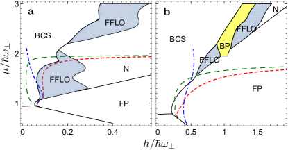
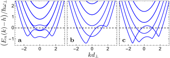
Figure 2 shows how the phase diagram changes at stronger interactions. As interactions favor pairing, we find superfluidity over a larger area. However, the phase diagram becomes more 3D-like, and the relative stabilities of different superfluid phases change. In particular, we see the appearance of a stable breached-pair (BP) phase near unitarity. As seen in the excitation spectra in Fig. 3a, the BP state is a gapless superfluid with a uniform order-parameter (in the direction), which contains both paired and unpaired modes. The unpaired fermions fill the sea of negative energy states. The literature (mostly on isotropic systems) distinguishes between BP states by the topology of the Fermi sea BPintro+detection ; BPintro+quarkmatter+BP1indeepBEC+topology ; BP1indeepBEC . For a given transverse quantum number, the Fermi sea in Fig. 3a is connected, making our state analogous to the “BP1” state in BPintro+detection . We do not find BP states where a Fermi sea is broken into disjoint momentum-intervals (cf. 3DsmallFFLO+BP1indeepBEC+detection+noncond ; 3DsmallFFLO+BPintro+BP1indeepBEC+detection ; 3DsmallFFLO+BPintro+BP1indeepBEC ; 3DsmallFFLO+BP1indeepBEC+noncond ; 3DsmallFFLO+BP1indeepBEC ; BPintro+quarkmatter+BP1indeepBEC+topology ; BPintro ; quasi1Dfinitesize+BP ; BP1indeepBEC ; interiorgap ; topology ; BP+display ). However, we do find FFLO states of both varieties (Fig. 3b-c). The BCS-BP transition, as well as the BP-FFLO transition are first-order, accompanied by jumps in the polarization.
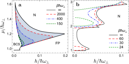
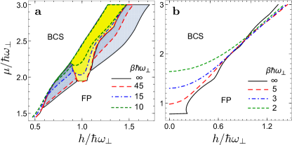
We show the phase diagrams at finite temperature in Figs. 4 and 5. Here we include thermal fluctuations at temperature by minimizing the mean-field free energy , where denotes the entropy. This has the effect of changing the sum in Eq. (4) to , where , and takes on both positive and negative values. Such a mean-field approach ignores the contribution of non-condensed pairs, and overestimates the critical temperature 3DsmallFFLO+BP1indeepBEC+detection+noncond ; 3DsmallFFLO+BP1indeepBEC+noncond ; fluctuations+noncond ; noncond+ ; noncond . However, we expect the qualitative features in Figs. 4 and 5 to be valid. In particular, we find vastly different critical temperatures for the FFLO and BCS phases, requiring separate figures to show the behavior. This separation of scales is reasonable, as the pairing energy of the gapped BCS phase is much larger than the gapless FFLO or BP phases. The critical temperatures grow with the interaction strength since the pairing energy is increased. The BCS phase acquires polarization at finite , which causes to decrease with , making the BCS-Normal transition second-order at small . At sufficiently high temperature the BP and BCS phases merge and become indistinguishable. The most striking feature of the weak-coupling phase diagram (Fig. 4) is that the BCS region breaks up into a series of disconnected lobes which disappear one by one at higher temperatures.
IV Derivation and comparison with an effective 1D model
To further understand this system, we take and map it onto an effective 1D model for . We project Eq. (3) into the harmonic oscillator basis, treating as a perturbation if or (where ). This yields a 1D BdG equation for the mode. Neglecting the influence of higher modes on the lowest mode yields an energy per unit length
| (7) |
where the integrals are over all , and the prime on the sum stands for . Here , and for , with . The first two terms in Eq. (7) separately diverge, but their sum is finite. This expression for maps to that of a purely 1D mean-field model provided we identify the effective 1D order parameter and the coupling constant as , and
| (8) |
Here , and when is even, and 0 otherwise, being a hypergeometric function. The prime on the sum now stands for . The expression in Eq. (8) converges as . The effective coupling constant is weakly dependent on , and its structure is best understood by taking , , for which
| (9) |
where denotes the Hurwitz zeta function, and is the unit step function. At , , which is Olshanii’s two-particle result mapping . As grows, decreases, approaching as . This divergence is unphysical, and signals a breakdown of the mapping to 1D when more channels open.
In Fig. 1b we evaluate the validity of this mapping by plotting the critical field of the BCS phase, , from the effective 1D model. It closely follows the critical field obtained from the full model for nearly all . We also plot using Olshanii’s mapping mapping , which agrees with the full model at small , but becomes less accurate as increases. Further, we show the prediction of the Bethe Ansatz with the mapping in Eq. (9), which illustrates the difference between an exact and a mean-field analysis in 1D 1DrichphasesMF+mapping+1Dphasediagram+exactvsMF . The mapping to 1D becomes less accurate at stronger interactions due to mixing of the trap levels, as seen in Fig. 2.
V Outlook
Achieving the temperatures required to directly observe the FFLO state at weak coupling is extremely challenging. The numbers near unitarity are more promising, but the accuracy of our mean-field theory is questionable there. The 1D thermodynamic measurements are promising 1Drichphases+1Dexperiment+1Dphasediagram . Time-dependent BdG calculations suggest the FFLO domain walls will be observable in time-of-flight expansion of 1D gases quasi1Dpromising+bolechFFLOdetection . This signature should be even more robust in the geometries we have been studying. There are also interesting connections to experiments on domain walls in highly elongated traps solitonvortex . It is likely that these various research directions will converge in the near future.
VI Acknowledgments
We thank Randy Hulet and Ben Olsen for useful discussions. This work was supported by the National Science Foundation under Grant PHY-1508300.
References
- (1) D. E. Sheehy and L. Radzihovsky, Phys. Rev. Lett. 96, 060401 (2006).
- (2) T. N. De Silva and E. J. Mueller, Phys. Rev. A 73, 051602(R) (2006); W. Yi and L.-M. Duan, ibid. 74, 013610 (2006).
- (3) M. M. Parish et al., Nat. Phys. 3, 124 (2007).
- (4) W. Yi and L.-M. Duan, Phys. Rev. A 73, 031604(R) (2006); X.-J. Liu and H. Hu, Europhys. Lett. 75, 364 (2006).
- (5) D. E. Sheehy and L. Radzihovsky, Ann. Phys. 322, 1790 (2007); L. Radzihovsky and D. E. Sheehy, Rep. Prog. Phys. 73, 076501 (2010); L. M. Jensen, J. Kinnunen, and P. Törmä, Phys. Rev. A 76, 033620 (2007); M. Mannarelli, G. Nardulli, and M. Ruggieri, ibid. 74, 033606 (2006); L. He, M. Jin, and P. Zhuang, Phys. Rev. B 73, 214527 (2006); C.-H. Pao, S.-T. Wu, and S.-K. Yip, ibid. 73, 132506 (2006); 74, 189901 (2006); A. Mishra and H. Mishra, Eur. Phys. J. D 53, 75 (2009).
- (6) N. Yoshida and S.-K. Yip, Phys. Rev. A 75, 063601 (2007); H. Hu and X.-J. Liu, ibid. 73, 051603(R) (2006).
- (7) X.-J. Liu, H. Hu, and P. D. Drummond, Phys. Rev. A 75, 023614 (2007).
- (8) X.-J. Liu, H. Hu, and P. D. Drummond, Phys. Rev. A 78, 023601 (2008); X.-W. Guan, M. T. Batchelor, and C. Lee, Rev. Mod. Phys. 85, 1633 (2013).
- (9) X.-J. Liu, H. Hu, and P. D. Drummond, Phys. Rev. A 76, 043605 (2007).
- (10) Y. Liao et al., Nature (London) 467, 567 (2010).
- (11) G. Orso, Phys. Rev. Lett. 98, 070402 (2007).
- (12) H. Hu, X.-J. Liu, and P. D. Drummond, Phys. Rev. Lett. 98, 070403 (2007).
- (13) G. G. Batrouni et al., Phys. Rev. Lett. 100, 116405 (2008); E. Zhao et al., ibid. 103, 140404 (2009); M. Tezuka and M. Ueda, ibid. 100, 110403 (2008); New J. Phys. 12, 055029 (2010); J.-S. He et al., ibid. 11 073009 (2009); P. Kakashvili and C. J. Bolech, Phys. Rev. A 79, 041603(R) (2009); M. J. Wolak et al., ibid. 82, 013614 (2010); F. Heidrich-Meisner, G. Orso, and A. E. Feiguin, ibid. 81, 053602 (2010); F. Heidrich-Meisner et al., ibid. 81, 023629 (2010); G. Xianlong and R. Asgari, ibid. 77, 033604 (2008); B. Wang and L.-M. Duan, ibid. 79, 043612 (2009); A. E. Feiguin and F. Heidrich-Meisner, Phys. Rev. B 76, 220508(R) (2007); A. E. Feiguin and D. A. Huse, ibid. 79, 100507(R) (2009); A-H. Chen and G. Xianlong, ibid. 85, 134203 (2012); E. Zhao and W. V. Liu, J. Low Temp. Phys. 158, 36 (2009); J. Y. Lee and X. W. Guan, Nucl. Phys. B 853, 125 (2011);
- (14) M. Rizzi, Phys. Rev. B 77, 245105 (2008).
- (15) M. Casula, D. M. Ceperley, and E. J. Mueller, Phys. Rev. A 78, 033607 (2008); S. K. Baur, J. Shumway, and E. J. Mueller, ibid. 81, 033628 (2010); A. Lüscher, R. M. Noack, and A. M. Läuchli, ibid. 78, 013637 (2008).
- (16) H. Müther and A. Sedrakian, Phys. Rev. Lett. 88, 252503 (2002); A. Sedrakian et al., Phys. Rev. A 72, 013613 (2005).
- (17) P. F. Bedaque, H. Caldas, and G. Rupak, Phys. Rev. Lett. 91, 247002 (2003); H. Caldas, Phys. Rev. A 69, 063602 (2004).
- (18) K. B. Gubbels and H. T. C. Stoof, Phys. Rep. 525, 255 (2013).
- (19) T.-L. Dao et al., Phys. Rev. Lett. 101, 236405 (2008).
- (20) Y.-L. Loh and N. Trivedi, Phys. Rev. Lett. 104, 165302 (2010); L. Radzihovsky, Phys. Rev. A 84, 023611 (2011); T. K. Koponen et al., New J. Phys. 10 045014 (2008).
- (21) C.-C. Chien et al., Phys. Rev. Lett. 97, 090402 (2006); 98, 110404 (2007); Phys. Rev. A 74, 021602(R) (2006); Y. He et al., ibid. 75, 021602(R) (2007); Q. Chen et al., ibid. 74, 063603 (2006).
- (22) A. Bulgac and M. M. Forbes, Phys. Rev. Lett. 101, 215301 (2008).
- (23) F. Chevy and C. Mora, Rep. Prog. Phys. 73, 112401 (2010); A. Bulgac, M. M. Forbes, and A. Schwenk, Phys. Rev. Lett. 97, 020402 (2006); K. Machida, T. Mizushima, and M. Ichioka, ibid. 97, 120407 (2006); K. B. Gubbels, M. W. J. Romans, and H. T. C. Stoof, ibid. 97, 210402 (2006); T. D. Cohen, ibid. 95, 120403 (2005); F. Chevy, ibid. 96, 130401 (2006); M. Iskin and C. A. R. Sá de Melo, ibid. 97, 100404 (2006); J. Carlson and S. Reddy, ibid. 95, 060401 (2005); T. Koponen et al., ibid. 99, 120403 (2007); S. Pilati and S. Giorgini, ibid. 100, 030401 (2008); P. Castorina et al., Phys. Rev. A 72, 025601 (2005); J.-P. Martikainen, ibid. 74, 013602 (2006); D. T. Son and M. A. Stephanov, ibid. 74, 013614 (2006); F. Chevy, ibid. 74, 063628 (2006); A. Bulgac and M. M. Forbes, ibid. 75, 031605(R) (2007); W.-C. Su, ibid. 74, 063627 (2006); Z. Zhang, ibid. 82, 033610 (2010); Z. Cai, Y. Wang, and C. Wu, ibid. 83, 063621 (2011); X. W. Guan et al., Phys. Rev. B 76, 085120 (2007); C.-H. Pao and S.-K. Kip, J. Phys. Condens. Matter 18, 5567 (2006); R. Combescot, Europhys. Lett. 55, 150 (2001); T. Koponen et al., New J. Phys. 8, 179 (2006); T.-L. Ho and H. Zhai, J. Low Temp. Phys. 148, 33 (2007); L. Radzihovsky, Physica C 481, 189 (2012); A. Koga and P. Werner, J. Phys. Soc. Jpn. 79, 064401 (2010).
- (24) L. Radzihovsky and A. Vishwanath, Phys. Rev. Lett. 103, 010404 (2009);
- (25) P. C. Hohenberg, Phys. Rev. 158, 383 (1967); N. D. Mermin and H. Wagner, Phys. Rev. Lett. 17, 1133 (1966).
- (26) P. Fulde and R. A. Ferrell, Phys. Rev. 135, A550 (1964); A. I. Larkin and Y. N. Ovchinnikov, Zh. Eksp. Teor. Fiz. 47, 1136 (1964) [Sov. Phys. JETP 20, 762 (1965)].
- (27) M. W. Zwierlein et al., Science 311, 492 (2006); G. B. Partridge et al., ibid. 311, 503 (2006); M. Zweierlein et al., Nature (London) 442, 54 (2006); Y. Shin et al., ibid. 451, 689 (2008); G. B. Partridge et al., Phys. Rev. Lett. 97, 190407 (2006); Y. Shin et al., ibid. 97, 030401 (2006).
- (28) M. M. Parish et al., Phys. Rev. Lett. 99, 250403 (2007).
- (29) R. M. Lutchyn, M. Dzero, and V. M. Yakovenko, Phys. Rev. A 84, 033609 (2011).
- (30) R. Mendoza, M. Fortes, and M. A. Solís, J. Low Temp. Phys. 175, 265 (2013).
- (31) H. Lu et al., Phys. Rev. Lett. 108, 225302 (2012).
- (32) H. Hu and X.-J. Liu, Phys. Rev. A 83, 013631 (2011); M. Swanson, Y. L. Loh, and N. Trivedi, New J. Phys. 14, 033036 (2012).
- (33) D.-H. Kim et al., Phys. Rev. Lett. 106, 095301 (2011).
- (34) L. O. Baksmaty et al., Phys. Rev. A 83, 023604 (2011); New J. Phys. 13 055014 (2011).
- (35) J. C. Pei, J. Dukelsky, and W. Nazarewicz, Phys. Rev. A 82, 021603(R) (2010).
- (36) X. Cui and Y. Wang, Phys. Rev. A 81, 023618 (2010).
- (37) W. Yi and L.-M. Duan, Phys. Rev. Lett. 97, 120401 (2006).
- (38) G. Sarma, J. Phys. Chem. Solids 24, 1029 (1963).
- (39) W. V. Liu and F. Wilczek, Phys. Rev. Lett. 90, 047002 (2003).
- (40) E. Gubankova, A. Schmitt, and F. Wilczek, Phys. Rev. B 74, 064505 (2006).
- (41) E. Zhao and W. V. Liu, Phys. Rev. A 78, 063605 (2008); K. Sun and C. J. Bolech, ibid. 87, 053622 (2013); 85, 051607(R) (2012).
- (42) K. Yang, Phys. Rev. B 63, 140511(R) (2001); A. E. Feiguin and F. Heidrich-Meisner, Phys. Rev. Lett. 102, 076403 (2009).
- (43) E. Gubankova, W. V. Liu, and F. Wilczek, Phys. Rev. Lett. 91, 032001 (2003); M. Alford, J. Berges, and K. Rajagopal, ibid. 84, 598 (2000); L. He, M. Jin, and P. Zhuang, Phys. Rev. D 74, 036005 (2006); J. A. Bowers and K. Rajagopal, ibid. 66, 065002 (2007); M. Alford, J. A. Bowers, and K. Rajagopal, ibid. 63, 074016 (2001); R. Casalbouni et al., ibid. 70, 054004 (2004); K. Rajagopal and A. Schmitt, ibid. 73, 045003 (2006); A. Sedrakian and D. H. Rischke, ibid. 80, 074022 (2009); I. Boettcher et al., Phys. Lett. B 742, 86 (2015); I. Giannakis, D.-f Hou, and H.-C. Ren, ibid. 631, 16 (2005); I. Shovkovy and M. Huang, ibid. 564, 205 (2003); M. Kitazawa, D. H. Rischke, and I. A. Shovkovy, ibid. 637, 367 (2006);
- (44) R. Casalbuoni and G. Nardulli, Rev. Mod. Phys. 76, 263 (2004).
- (45) H. A. Radovan et al., Nature (London) 425, 51 (2003); M. Kenzelmann et al., Science 321, 1652 (2008); A. I. Buzdin and S. V. Polonskii, Zh. Eksp. Teor. Fiz. 93, 747 (1987) [Sov. Phys. JETP 66, 422 (1987)]; L. W. Gruenberg and L. Gunther, Phys. Rev. Lett. 16, 996 (1966); K. Kakuyanagi et al., ibid. 94, 047602 (2005); C. F. Miclea et al., ibid. 96, 117001 (2006); A. Bianchi et al. ibid. 91, 187004 (2003); G. Koutroulakis et al., ibid. 104, 087001 (2010); K. Kumagai et al., ibid. 97, 227002 (2006); S. Uji et al., ibid. 97, 157001 (2006); R. Lortz et al., ibid. 99, 187002 (2007); S. Yonezawa et al., ibid. 100, 117002 (2008); T. Kontos et al., ibid. 86, 304 (2001); Y. L. Loh et al., ibid. 107, 067003 (2011); S. K. Sinha et al., ibid. 48, 950 (1982); H. Burkhardt and D. Rainer, Ann. Phys. (Leipzig), 3, 181 (1994); K. Machida and H. Nakanishi, Phys. Rev. B 30, 122 (1984); M. Houzet and A. Buzdin, ibid. 63, 184521 (2001); N. Dupuis, ibid. 51, 9074 (1995); A. G. Lebed and S. Wu, ibid. 82, 172504 (2010); H. Shimahara, ibid. 50, 12760 (1994); T. Watanabe et al., ibid. 70, 020506(R) (2004); C. Capan et al., ibid. 70, 134513 (2004); B. Bergk et al., ibid. 83, 064506 (2011); S. Uji et al., ibid. 85, 174530 (2012); K. Cho et al., ibid. 79, 220507(R) (2009); Y. Matsuda and H. Shimahara, J. Phys. Soc. Jpn. 76, 051005 (2007); M. Nicklas et al., ibid. 76, 128 (2007); S. Yonezawa et al., ibid. 77, 054712 (2008); I. T. Padilha and M. A. Continentino, J. Phys. Condens. Matter 21 095603 (2009); J. Singleton et al., ibid. 12, L641–L648 (2000); J. A. Symington et al., Physica B 294, 418 (2001); G. Zwicknagl and J. Wosnitza, Int. J. Mod. Phys. B 24, 3915 (2010);
- (46) H. Mayaffre et al., Nat. Phys. 10, 928 (2014).
- (47) Z. Koinov, R. Mendoza, and M. Fortes, Phys. Rev. Lett. 106, 100402 (2011); W. Ong et al., ibid. 114, 110403 (2015); M. M. Parish and J. Levinsen, Phys. Rev. A 87, 033616 (2013); J. P. A. Devreese, S. N. Klimin, and J. Tempere, ibid. 83, 013606 (2011); J. P. A. Devreese, M. Wouters, and J. Tempere, ibid. 84, 043623 (2011); S. Yin, J.-P. Martikainen, and P. Törmä, Phys. Rev. B 89, 014507 (2014); A. V. Samokhvalov, A. S. Mel’nikov, and A. I. Buzdin, ibid. 82, 174514 (2010); T. N. De Silva, J. Phys. B: At. Mol. Opt. Phys. 42, 165301 (2009); D. E. Sheehy, arXiv:1407.8021 (2015).
- (48) C. Chin et al., Rev. Mod. Phys. 82, 1225 (2010).
- (49) M. Olshanii, Phys. Rev. Lett. 81, 938 (1998); T. Bergeman, M. G. Moore, and M. Olshanii, ibid. 91, 163201 (2003).
- (50) R. Dasgupta, Phys. Rev. A 80, 063623 (2009).
- (51) A. Bulgac and M. M. Forbes, arXiv:0808.1436 (2008); A. Bulgac, M. M. Forbes, and P. Magierski, ibid.:1008.3933 (2012).
- (52) A. Perali et al., Phys. Rev. Lett. 92, 220404 (2004); J. Tempere, S. N. Klimin, and J. T. Devreese, Phys. Rev. A 78, 023626 (2008); I. Boettcher et al., ibid. 91, 013610 (2015); E. J. Mueller, ibid. 83, 053623 (2011).
- (53) M. M. Forbes et al., Phys. Rev. Lett. 94, 017001 (2005).
- (54) S.-T. Wu and S. Yip, Phys. Rev. A 67, 053603 (2003); P. Hor̆ava, Phys. Rev. Lett. 95, 016405 (2005); Y. X. Zhao and Z. D. Wang, ibid. 110, 240404 (2013); J. L. Mañes, F. Guinea, and M. A. H. Vozmediano, Phys. Rev. B 75, 155424 (2007); G. E. Volovik, arXiv:cond-mat/0601372 (2006).
- (55) C. J. Bolech et al., Phys. Rev. Lett. 109, 110602 (2012); M. Reza Bakhtiari, M. J. Leskinen, and P. Törmä, ibid. 101, 120404 (2008); C. Sanner et al., ibid. 106, 010402 (2011); J. M. Edge and N. R. Cooper, ibid. 103, 065301 (2009); T. Mizushima, K. Machida, and M. Ichioka, ibid. 94, 060404 (2005); A. Korolyuk, F. Massel, and P. Törmä, ibid. 104, 236402 (2010); G. M. Bruun et al., ibid. 102, 030401 (2009); J. Kinnunen, L. M. Jensen, and P. Törmä, ibid. 96, 110403 (2006); K. Yang, ibid. 95, 218903 (2005); arXiv:cond-mat/0603190 (2007); J. Kajala, F. Massel, and P. Törmä, Phys. Rev. A 84, 041601(R) (2011); V. Gritsev, E. Demler, and A. Polkovnikov, ibid. 78, 063624 (2008); E. Altman, E. Demler, and M. D. Lukin, ibid. 70, 013603 (2004); T. Paananen et al., ibid. 77, 053602 (2008); Y.-P. Shim, R. A. Duine, and A. H. MacDonald, ibid. 74, 053602 (2006); M. O. J. Heikkinen and P. Törmä, ibid. 83, 053630 (2011); J. T. Stewart, J. P. Gaebler, and D. S. Jin, Nature (London) 454, 744 (2008); K. Eckert et al., Nat. Phys. 4, 50 (2008); T. Rosclide et al., New J. Phys. 11, 055041 (2009).
- (56) H. T. C. Stoof, K. B. Gubbels, and D. B. M. Dickerscheid, Ultracold Quantum Fields (Springer, Dordrecht, 2009).
- (57) G. Bruun et al., Eur. Phys. J. D 7, 433 (1999); A. Bulgac and Y. Yu, Phys. Rev. Lett. 88, 042504 (2002); M. Grasso and M. Urban, Phys. Rev. A 68, 033610 (2003).
- (58) Y. He et al., Phys. Rev. B 76, 224516 (2007).
- (59) M. J. H. Ku et al., Phys. Rev. Lett. 113, 065301 (2014); T. Yesfah et al., Nature (London) 499, 426 (2013).