Classically and Quantum stable Emergent Universe from Conservation Laws

Abstract

It has been recently pointed out by Mithani-Vilenkin Mithani:2014jva ; Mithani:2011en ; Mithani:2012ii ; Mithani:2014toa that certain emergent universe scenarios which are classically stable are nevertheless unstable semiclassically to collapse. Here, we show that there is a class of emergent universes derived from scale invariant two measures theories with spontaneous symmetry breaking (s.s.b) of the scale invariance, which can have both classical stability and do not suffer the instability pointed out by Mithani-Vilenkin towards collapse.

We find that this stability is due to the presence of a symmetry in the ”emergent phase”, which together with the non linearities of the theory, does not allow that the FLRW scale factor to be smaller that a certain minimum value $a_{0}$ in a certain protected region.

The standard hot big-bang model provides us with the description of how the universe evolves, explaining the observational facts, such as the Hubble expansion, the $3K$ microwave background radiation and the abundance of light elements. However, this model presents some problems in its evolution. We will reference some of then; the smoothness or horizon problem, the flatness, the structure or primordial density problem, etc.. These problems can be solved in the context of the inflationary universe Guth , where the essential feature of any inflationary model is the rapid but finite period of expansion that the universe underwent at very early times in its evolution. Perhaps the most import feature of the inflationary universe model is that it provides a causal explication for the origin of the observed anisotropy in the cosmic microwave background radiation (CMB), and also to the distribution of large-scale structures, which are consistent with the observations Larson ; Planck .

However, one should point out that even in the context of the inflationary scenario one still encounters the initial singularity problem singular ; HE-book showing that the universe necessarily had a singular beginning for generic inflationary cosmologies Borde-Vilenkin-PRL .

One interesting way to avoid the initial singularity problem is to consider the emergent universe (EU) scenario orgemm . The emergent universe refers to models in which the universe emerges from a past eternal Einstein static state (ES), inflates, and then evolves into a hot big bang era. The EU is an attractive scenario since it avoids the initial singularity and provides a smooth transition towards an inflationary period.

The original proposal for the emergent universe orgemm supported an instability at the classical level of the ES state, and various models intended to formulate a stable model have been given emm2 , in particular the Jordan Brans Dicke models emm3 . In this context, Mithani-Vilenkin in Refs. Mithani:2011en -Mithani:2014toa have shown that certain classically stable static universes could be unstable semiclassically towards collapse. In this work, we show that there is a class of emergent universes derived from scale invariant two measures theories with spontaneous symmetry breaking of the scale invariance, which can have both classical stability and do not suffer the instability pointed out by Mithani-Vilenkin towards collapse of the ES state.

In a series of papers prev -Guendelman:2014bva we have studied a class of EU scenarios which are based on a spontaneously broken scale symmetry induced by the dynamics of a Two Measures Field Theory (TMT)GK1 -GK8 , (see also Ref.prev ). In such model there is a dilaton field $\phi$ and the EU as the $t\longrightarrow-\infty$ is well described by an Einstein static universe, where $t$ is the cosmological time.

In the Appendix A, we have included a summary of the principal characteristic of the TMT theories. Here we want to consider the detailed analysis of the EU solutions of the model developed in Ref. yo . The results obtained in this case can also be applied to models studied in Refs. prev -Guendelman:2014bva , which present similar symmetries as the model in Ref. yo .

We start by considering the Friedmann-Robertson-Walker closed cosmological solutions of the form

$$ds^{2}=dt^{2}-a(t)^{2}\left(\frac{dr^{2}}{1-r^{2}}+r^{2}(d\theta^{2}+sin^{2}\theta d\phi^{2})\right),\phi=\phi(t),$$ (1)

where $a(t)$ is the scale factor, and the scalar field $\phi$ is a function of the cosmic time $t$ only, due to homogeneously and isotropy. We will consider a scenario where the scalar field $\phi$ is moving in the extreme left region $\phi\rightarrow-\infty$. In this case, the expressions for the energy density $\rho$ and pressure $p$ are given by

$$\rho=\frac{A}{2}\dot{\phi}^{2}+3B\dot{\phi}^{4}+C,$$ (2)

and

$$p=\frac{A}{2}\dot{\phi}^{2}+B\dot{\phi}^{4}-C,$$ (3)

see Appendix A. Where the constants $A,B$ and $C$ are given by,

$$A=1-\frac{2\delta b_{g}V_{1}}{4(b_{g}V_{1}-V_{2})}\,,\,\,\,\,B=-\frac{\delta^{2}b^{2}_{g}}{4(b_{g}V_{1}-V_{2})}\,,\,\,\,\,\mbox{and}\,\,\,\,C=\frac{V^{2}_{1}}{4(b_{g}V_{1}-V_{2})}\,.$$ (4)

As was discussed in Ref.yo , the emergent universe can turn into inflation only if $C>0$. On the other hand, in order to have a scenario in which the emergent universe evolves from an static and classically stable universe at $a=a^{*}$ with

$$a^{*}=\sqrt{\left(\frac{3}{8\pi G}\right)\frac{12B}{A^{2}+24B\,C-A\sqrt{A^{2}+12B\,C}}}\,\,,$$ (5)

and then passed to an inflationary phase, the following conditions must to be met, see Ref. yo :

$$0.5<y<0.54\,,$$ (6)

$$B<0\,,$$ (7)

$$-\frac{1}{64B}<C<-\sqrt{\frac{3}{B^{2}}}-\frac{7}{4B}\,.$$ (8)

Where $A=1-y$ and we have defined $y=\frac{2\delta b_{g}C}{V_{1}}$.

Now will turn our attention to possible quantum tunneling from the solution $a=a^{*}$ to $a=0$, during the static regimen of the EU scenario. Let us first note that there is a conserved quantity $\Pi_{\phi}$, due to the fact that from $\phi\rightarrow-\infty$, there is other symmetry $\phi\rightarrow\phi+c$. Given that in the Einstein frame we can use the action

$$S=\frac{1}{\kappa}\left[\int\,R\,\sqrt{-g}\,d^{4}x\,+\,\int\,p\,\sqrt{-g}\,d^{4}x\right],$$ (9)

and the symmetry $\phi\rightarrow\phi+c$, in which c is a constant, leads to the conservation law

$$a^{3}(t)\,[A\dot{\phi}+4\,B\dot{\phi}^{3}]=\Pi_{\phi}=const.\,.$$ (10)

Without loss of generality, let us consider $\Pi_{\phi}>0$, see Appendix B for the case $\Pi_{\phi}<0$. From conservation equation (10), we can write $a$ as a function of $\dot{\phi}$

$$a(\dot{\phi})=\left(\frac{\Pi_{\phi}}{A\dot{\phi}+4\,B\dot{\phi}^{3}}\right)^{1/3}.$$ (11)

We can note that in this case $-\infty<\dot{\phi}<-\sqrt{\frac{A}{4|B|}}$ or $0<\dot{\phi}<\sqrt{\frac{A}{4|B|}}$ in order to satisfied $\Pi_{\phi}>0$. When $\dot{\phi}$ is in the first region $a(\dot{\phi})$ is a function which approach to zero when $\dot{\phi}\rightarrow-\infty$ and diverges when $\dot{\phi}\rightarrow-\sqrt{\frac{A}{4|B|}}$. But in this region $\rho$ becomes negative see Eq. (2), then we are not interested in this case.

On the other hand, when $\dot{\phi}$ is in the second region, $a(\dot{\phi})$ has an extremum (minimum) at $\dot{\phi}=\dot{\phi}_{0}$, where $a(\dot{\phi}_{0})=a_{0}$, with

$$\dot{\phi}_{0} = \sqrt{\frac{A}{12|B|}}\,,$$ (12)

$$a_{0} = \left(\frac{12|B|}{A}\right)^{1/6}\left[\frac{3\Pi_{\phi}}{2A}\right]^{1/3}\,.$$ (13)

Also from Eq. (11), we obtain that in this region $a$ diverges when $\dot{\phi}$ approach to zero or to $\sqrt{\frac{A}{4|B|}}$.

Therefore, we can note that a smaller scale factor than $a_{0}$ is out of the range where the scale factor is defined for the physical solutions.

As an example, in Fig. 1 we have plotted $a(\dot{\phi})$, where we have considered $B=-1$, $C=0.016$, $y=0.505964$ and $\Pi_{\phi}=113.41$.

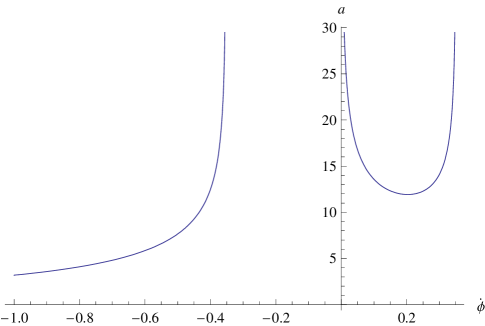
Figure 1: From Eq. (10), the scale factor $a$ as a function of $\dot{\phi}$, when it is consider $\Pi_{\phi}=113.41$.

From Eq. (10) we can obtain $\dot{\phi}$ as a function of $a$. We have three solutions:

$$\dot{\phi}_{1} = -\frac{a^{3}A}{2\,3^{1/3}\left(9a^{6}B^{2}\Pi_{\phi}+\sqrt{3}\sqrt{a^{18}A^{3}B^{3}+27a^{12}B^{4}\Pi_{\phi}^{2}}\right)^{1/3}}$$

$$+\frac{\left(9a^{6}B^{2}\Pi_{\phi}+\sqrt{3}\sqrt{a^{18}A^{3}B^{3}+27a^{12}B^{4}\Pi_{\phi}^{2}}\right)^{1/3}}{2\,3^{2/3}a^{3}B}\,,$$

$$\dot{\phi}_{2} = \frac{\left(1+i\sqrt{3}\right)a^{3}A}{43^{1/3}\left(9a^{6}B^{2}\Pi_{\phi}+\sqrt{3}\sqrt{a^{18}A^{3}B^{3}+27a^{12}B^{4}\Pi_{\phi}^{2}}\right)^{1/3}}$$

$$-\frac{\left(1-i\sqrt{3}\right)\left(9a^{6}B^{2}\Pi_{\phi}+\sqrt{3}\sqrt{a^{18}A^{3}B^{3}+27a^{12}B^{4}\Pi_{\phi}^{2}}\right)^{1/3}}{43^{2/3}a^{3}B}\,,$$

$$\dot{\phi}_{3} = \frac{\left(1-i\sqrt{3}\right)a^{3}A}{43^{1/3}\left(9a^{6}B^{2}\Pi_{\phi}+\sqrt{3}\sqrt{a^{18}A^{3}B^{3}+27a^{12}B^{4}\Pi_{\phi}^{2}}\right)^{1/3}}$$

$$-\frac{\left(1+i\sqrt{3}\right)\left(9a^{6}B^{2}\Pi_{\phi}+\sqrt{3}\sqrt{a^{18}A^{3}B^{3}+27a^{12}B^{4}\Pi_{\phi}^{2}}\right)^{1/3}}{43^{2/3}a^{3}B}\,.$$

As an example we plot these solutions in Figs. (2, 3, 4), where we have used the values of Ref. yo and $\Pi_{\phi}=113.41$. We can note that the plots are fully consistent with Fig. 1.

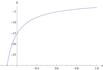
Figure 2: From Eq. (10), $\dot{\phi}_{1}$ as function of $a$ when it is consider $\Pi_{\phi}=113.41$.

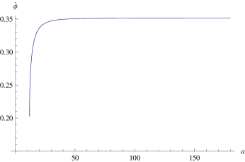
Figure 3: From Eq. (10), $\dot{\phi}_{2}$ as function of $a$ when it is consider $\Pi_{\phi}=113.41$.

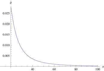
Figure 4: From Eq. (10), $\dot{\phi}_{3}$ as function of $a$ when it is consider $\Pi_{\phi}=113.41$.

The classical theory which describe this universe can be regarded as a constrained dynamical system with a Hamiltonian

$${\cal H}=-\frac{G}{3\pi\,a}\left(p^{2}_{a}+U(a)\right),$$ (17)

where

$$p_{a}=-\frac{3\pi}{2G}\,a\,\dot{a},$$ (18)

is the momentum conjugate to $a$, and $U(a)$ corresponds to the effective potential given by

$$U(a)=\left(\frac{3\pi}{2G}\right)a^{2}\left(1-\frac{8\pi G}{3}\,a^{2}\,\rho(a)\right),$$ (19)

where we have written $\rho$ as a function of $a$. It is possible to do that by using the solutions Eqs.(Classically and Quantum stable Emergent Universe from Conservation Laws, Classically and Quantum stable Emergent Universe from Conservation Laws, Classically and Quantum stable Emergent Universe from Conservation Laws) and Eq. (2).

The Hamiltonian constraint is ${\cal H}=0$, from where we obtain the Friedmann equation

$$\left(\frac{\dot{a}}{a}\right)^{2}=\frac{8\pi G}{3}\,\rho(a)-\frac{1}{a^{2}}\,.$$ (20)

Also, we can obtain the equation for $\dot{H}$ given by

$$\dot{H}=-4\pi\,G(\rho+p)+\frac{1}{a^{2}}\,.$$ (21)

One of the characteristic of the EU scenario is the period of superinflation after de static regimen and before inflation where ($\dot{H})>0$, see Labrana:2013oca . From Eq. (21), we note that in the relevant solutions of our model we do not need to violate the null energy condition, $\rho+p>0$, in order to have an EU scenario (with a superinflationary phase) and avoid the initial singularity, since we are considering a closed universe. This is different from what happens in models as Ref. Rubakov:2014jja , which by the way shows that some violations of the energy conditions can be consistent.

In the context of quantum theory, the universe could be described by a wave function $\psi(a)$, the conjugate momentum $p_{a}$ becomes the differential operator $-id/da$ and the constraint is replaced by the Wheeler-DeWitt (WDW) equation Will

$${\cal H}\psi(a)=0,$$ (22)

$$\left(-\frac{d^{2}}{da^{2}}-\frac{\beta}{a}\,\frac{d}{da}+U(a)\right)\psi(a)=0\,,$$ (23)

where we have used the minisuperspace approximation, which is appropriated for our model where the universe is homogeneous isotropic and closed during the ES regimen and therefore has a single degree of freedom, the scale factor Vilenkin:1987kf . The parameter $\beta$ represents the ambiguity in the ordering of the non-commuting factors $a$ and $p_{a}$ in the Hamiltonian. The value of $\beta$ does not affect the wave function in the semiclassical regimen, and usually in the study of semi-classical stability of EU it is chosen to be zero, see Mithani:2011en ; Mithani:2012ii ; Mithani:2014jva ; Mithani:2014toa .

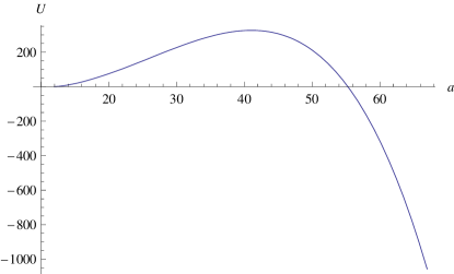
Figure 5: Potential $U(a)$ for $a>a_{0}$. Here, we have used Eq. (Classically and Quantum stable Emergent Universe from Conservation Laws).

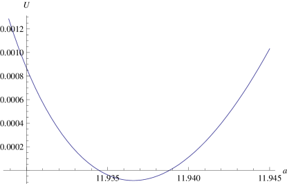
Figure 6: Potential $U(a)$ for $a>a_{0}$ near the equilibrium point. Here, we have used Eq. (Classically and Quantum stable Emergent Universe from Conservation Laws).

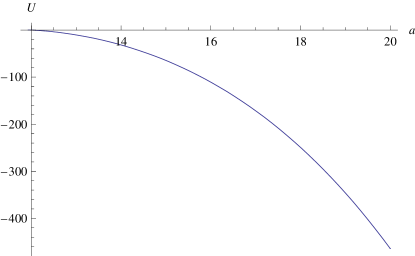
Figure 7: Potential $U(a)$ for $a>a_{0}$. Here, we have used Eq. (Classically and Quantum stable Emergent Universe from Conservation Laws).

In order to obtain the potential $U(a)$ for the case of the EU, we have to select one of the solutions Eqs.(Classically and Quantum stable Emergent Universe from Conservation Laws, Classically and Quantum stable Emergent Universe from Conservation Laws, Classically and Quantum stable Emergent Universe from Conservation Laws) which is related with the static and classically stable solution. This classical solution was discussed in Ref. yo . In this case this solution is Eq. (Classically and Quantum stable Emergent Universe from Conservation Laws). When we consider this solution the potential $U(a)$ has a local minimum at $a=a^{*}$, where $a^{*}$ was defined in Eq. (5) and a local maximum at $a=a^{\prime}$, where

$$a^{\prime}=\sqrt{\left(\frac{3}{8\pi G}\right)\frac{12B}{A^{2}+24B\,C+A\sqrt{A^{2}+12B\,C}}}\,\,.$$ (24)

The nature of these two equilibrium points was discussed in Ref.yo , where it is shown that $a=a^{*}$ is an stable equilibrium point and $a=a^{\prime}$ is an unstable equilibrium point. Then, the system is classically stable near the static solution, $a\sim a^{*}$. There is a finite barrier which prevents the scale factor to go from $a\simeq a^{*}$ to infinity and the potential is not well defined for $a<a_{0}$ given the discussion above, this can be interpreted as a hard wall at $a=a_{0}$ for the potential $U(a)$.

As an example, in Fig. 5 it is plot the potential for the values allowed for $a$, that is $a>a_{0}$. In Fig. 6 it is plot the potential $U(a)$ near the static point (where also was consider $a>a_{0}$).

Since a smaller scale factor than $a_{0}$ is out of the range where the scale factor is defined for the physical solutions, we find that the possible instability towards $a$ equal zero is not even a logical possibility in this context. Nevertheless, we observe that exist the possibility of tunneling through the finite barrier from the static solution to an expanding universe, see Fig. 5. This is an interesting scenario to study in future works.

As an example, in Fig. 7 it is show the potential for the solution Eq. (Classically and Quantum stable Emergent Universe from Conservation Laws), we can note, as we expected, that in this case there is not a equilibrium point as in Fig. 6.

From the Friedmann equation, Eq. (20), and Eq. (10) we can note that solutions $\dot{\phi}_{2}$ and $\dot{\phi}_{3}$ are not connected by the dynamics of the system. Solution Eq. (Classically and Quantum stable Emergent Universe from Conservation Laws) satisfies $\dot{\phi}_{2}>\dot{\phi}_{0}$ and solution Eq. (Classically and Quantum stable Emergent Universe from Conservation Laws) satisfies $\dot{\phi}_{3}<\dot{\phi}_{0}$, and it is not possible to cross the line $\dot{\phi}=\dot{\phi}_{0}$. At this respect, and by using Eq.(10), we can rewrite Eq. (20) as the following equations for $\dot{\phi}$,

$$\ddot{\phi}^{2}+V(\dot{\phi})=0\,,$$ (25)

where

$$V(\dot{\phi})=\frac{(A\dot{\phi}+4B\dot{\phi}^{3})^{2}}{(A+12B\dot{\phi}^{2})^{2}}\,\left[\frac{1}{\Pi_{\phi}^{2/3}}(A\dot{\phi}+4B\dot{\phi}^{3})^{2/3}-\frac{\kappa}{3}\,\left(\frac{A}{2}\dot{\phi}^{2}+3B\dot{\phi}^{4}+C\right)\right].$$ (26)

Then, from Eq. (26) we note that the solutions $\dot{\phi}_{2}$ and $\dot{\phi}_{3}$ are classically disconnected since $V\rightarrow\infty$ at the value $\dot{\phi}=\dot{\phi}_{0}=\sqrt{\frac{A}{12|B|}}$. However, there is the possibility of tunneling through this divergent barrier, see Dittrich:1986ef . In this case, the tunneling correspond to a quantum tunneling from the static solution to an expanding universe with initial values $a=a_{0}$.

As an example in Fig. 8 it is shown the potential $V(\dot{\phi})$, where we have used $\Pi_{\phi}=113.41$ and the values of Ref. yo . We can note that there is an infinite barrier at $\dot{\phi}=\dot{\phi}_{0}=0.20$.

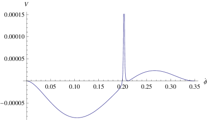
Figure 8: Potential $V(\dot{\phi})$, for $\dot{\phi}>0$.

In Fig. 9 we show the dependence of the potential $V(\dot{\phi})$ as a function of $\dot{\phi}$, near the equilibrium point.

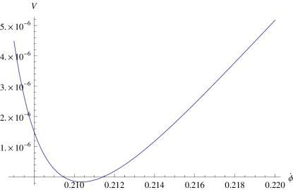
Figure 9: Potential $V(\dot{\phi})$ near the equilibrium point.

Therefore, we note that both tunnelings discussed above do not correspond to a collapse to $a\rightarrow 0$, but a creation of an expanding universe.

I Discussion and Conclusions

It has been recently pointed out by Mithani-Vilenkin Mithani:2014jva ; Mithani:2011en ; Mithani:2012ii ; Mithani:2014toa that certain emergent universe scenarios which are classically stable are nevertheless unstable semiclassically to collapse. In this work, we shown that there is a class of emergent universes derived from scale invariant two measures theories with spontaneous symmetry breaking of the scale invariance, which can have both classical stability and do not suffer the instability pointed out by Mithani-Vilenkin towards collapse. This stability is due to the presence of a symmetry in the ”emergent phase”, which together with the non linearities of the theory, does not allow the FLRW scale factor to be smaller that a certain minimum $a_{0}$ in a certain protected region.

Since a smaller scale factor than $a_{0}$ is out of the range where it is defined for the physical solutions $\dot{\phi}_{2}$ and $\dot{\phi}_{3}$ where $\rho$ is positive, we have found that the possible instability towards a scale factor equal zero is not even a logical possibility in this context. Therefore our model is free of the instability towards collapse described in Refs. Mithani:2014jva ; Mithani:2011en ; Mithani:2012ii ; Mithani:2014toa . The conserved quantity $\Pi_{\phi}\neq 0$ provides in this case with a protection towards collapse to $a$ equal zero.

It is interesting to observe that exist the possibility of tunneling through the finite barrier of the potentials $U(a)$ and $V(\dot{\phi})$ from the static solution to an expanding universe, but also there is the possibility of tunneling through the divergent barrier of potentials $V(\dot{\phi})$, see Eq. (26). In this case, the tunneling correspond to a quantum tunneling from the static solution to an expanding universe with initial values $a=a_{0}$. We have noted that both tunnelings process, do not correspond to a collapse to $a\rightarrow 0$, instead they correspond to a creation of an expanding universe. This is an interesting scenario to study in future works and correspond to an alternative scheme for an emergent universe scenario, similar to the one studied in Refs. Labrana:2011np .

In particular in this work we studied the model Ref. yo , but the results obtained in this work can also be applied to models studied in Refs. prev -Guendelman:2014bva , which present similar symmetries as the model in Ref. yo .

We should mention that, we have considered a closed universe, where the contribution of the curvature term is relevant before the inflationary period. Nevertheless, they are the possibility of contrast the EU with observation by studying the superinflationary period of these models. As it was reported in Ref. Labrana:2013oca , during the superinflationary period, the EU scenario produces a suppression of the CMB anisotropies at large scale which could be responsible for the observed lack of power at large angular scales of the CMB. We hope to be able to analyze this suppression and also submitting our model to further test such as CMB temperature anisotropies and density perturbations. This will be the subject of a future work.

II Acknowledgements

The authors dedicate this article to the memory of Professor Sergio del Campo (R.I.P.).

We thank Professor Alexander Vilenkin for suggesting and encouraging us to study the problem of the quantum stability of the emergent universe scenario and for multiple discussions on this subject. This work was supported by Comisión Nacional de Ciencias y Tecnología through FONDECYT Grants 1110230 (SdC), 1130628 (RH). Also it was supported by Pontificia Universidad Católica de Valparaíso through grants 123.787-2007 (SdC) and 123724 (RH). One of us (E.I.G) would like to thank the astrophysics and cosmology group at the Pontificia Universidad Católica de Valparaíso and the Frankfurt Institute of Advanced Studies of Frankfurt University for hospitality. P. L. is supported by Dirección de Investigación de la Universidad del Bío-Bío through Grants N⁰ 166907 2/R, and GI 150407/VC.

Appendix A: Review of the TMT theories

The TMT is a generally coordinate invariant theory, where the action has to be of the formGK3 -GK8

$$S=\int L_{1}\Phi d^{4}x+\int L_{2}\sqrt{-g}d^{4}x,$$ (27)

including two Lagrangians $L_{1}$ and $L_{2}$ and two measures of integration $\sqrt{-g}$ and $\Phi$. One is the usual measure of integration $\sqrt{-g}$ in the 4-dimensional space-time manifold equipped with the metric $g_{\mu\nu}$. The other is the new measure of integration $\Phi$ in the same 4-dimensional space-time manifold. The measure $\Phi$ being a scalar density and a total derivative (see Ref.Mstring ) may be defined by means of four scalar fields $\varphi_{a}$ ($a=1,2,3,4$),

$$\Phi=\varepsilon^{\mu\nu\alpha\beta}\varepsilon_{abcd}\partial_{\mu}\varphi_{a}\partial_{\nu}\varphi_{b}\partial_{\alpha}\varphi_{c}\partial_{\beta}\varphi_{d}.$$ (28)

It is assumed that the Lagrangian densities $L_{1}$ and $L_{2}$ are functions of all matter fields, the dilaton field, the metric, the connection but not of the ”measure fields” ($\varphi_{a}$ ). In such a case, i.e. when the measure fields enter in the theory only via the measure $\Phi$, the action (27) possesses an infinite dimensional symmetry. In the case given by Eq.(28) these symmetry transformations have the form $\varphi_{a}\rightarrow\varphi_{a}+f_{a}(L_{1})$, where $f_{a}(L_{1})$ are arbitrary functions of $L_{1}$ (see details in Ref.GK3 ).

In this theory, we assume that all fields, including also the metric, connection and the measure fields are independent dynamical variables. All the relations among them are results of the equations of motion. In particular, the independence of the metric and the connection means that we proceed in the first order formalism and the relation between connection and metric is not necessarily according to Riemannian geometry.

Varying the measure fields $\varphi_{a}$, we get $B^{\mu}_{a}\partial_{\mu}L_{1}=0$ where $B^{\mu}_{a}=\varepsilon^{\mu\nu\alpha\beta}\varepsilon_{abcd}\partial_{\nu}\varphi_{b}\partial_{\alpha}\varphi_{c}\partial_{\beta}\varphi_{d}.$ Since $Det(B^{\mu}_{a})=\frac{4^{-4}}{4!}\Phi^{3}$ it follows that if $\Phi\neq 0$,

$$L_{1}=sM^{4}=const,$$ (29)

where $s=\pm 1$ and $M$ is a constant of integration with the dimension of mass.

We proceed now to discuss the question of scale invariance in the context of TMT. A dilaton field $\phi$ allows to realize a spontaneously broken global scale invarianceG1 . We postulate that the theory is invariant under the global scale transformations:

$$g_{\mu\nu}\rightarrow e^{\theta}g_{\mu\nu},\quad\Gamma^{\mu}_{\alpha\beta}\rightarrow\Gamma^{\mu}_{\alpha\beta},\quad\varphi_{a}\rightarrow\lambda_{ab}\varphi_{b}\quad\text{where}\quad\det(\lambda_{ab})=e^{2\theta},\quad\phi\rightarrow\phi-\frac{M_{p}}{\alpha}\theta.$$ (30)

We choose an action which, except for the modification of the general structure caused by the basic assumptions of TMT, does not contain any exotic terms and fields as like as in the conventional formulation of the minimally coupled scalar-gravity system. Keeping the general structure (27), it is convenient to represent the underlying action of our model in the following form GKKess :

$$S = \int d^{4}xe^{\alpha\phi/M_{p}}\Big{[}-\frac{1}{2\,\kappa}R(\Gamma,g)(\Phi+b_{g}\sqrt{-g})+(\Phi+b_{\phi}\sqrt{-g})\frac{1}{2}g^{\mu\nu}\phi_{,\mu}\phi_{,\nu}$$

$$- e^{\alpha\phi/M_{p}}\left(\Phi V_{1}+\sqrt{-g}V_{2}\right)\Big{]}.$$

We use $\kappa=8\pi/M_{p}^{2}$ where $M_{p}$ is the four-dimensional Planck mass. In the equations of motion following from this action, we change the metric to the new one

$$\tilde{g}_{\mu\nu}=e^{\alpha\phi/M_{p}}(\zeta+b_{g})g_{\mu\nu},$$ (32)

where $\zeta\equiv\frac{\Phi}{\sqrt{-g}}$. The conformal metric $\tilde{g}_{\mu\nu}$ represents the ”Einstein frame”, since the connection becomes Riemannian. Notice that $\tilde{g}_{\mu\nu}$ is invariant under the scale transformations (30). After the change of variables to the Einstein frame the gravitational equations take the standard GR form

$$G_{\mu\nu}(\tilde{g}_{\alpha\beta})=\kappa\,T_{\mu\nu}^{eff},$$ (33)

where $G_{\mu\nu}(\tilde{g}_{\alpha\beta})$ is the Einstein tensor. The energy-momentum tensor, $T_{\mu\nu}^{eff}$, becomes

$$T_{\mu\nu}^{eff} = \frac{\zeta+b_{\phi}}{\zeta+b_{g}}\left(\phi_{,\mu}\phi_{,\nu}-\frac{1}{2}\tilde{g}_{\mu\nu}\tilde{g}^{\alpha\beta}\phi_{,\alpha}\phi_{,\beta}\right)-\tilde{g}_{\mu\nu}\frac{b_{g}-b_{\phi}}{2(\zeta+b_{g})}\tilde{g}^{\alpha\beta}\phi_{,\alpha}\phi_{,\beta}+\tilde{g}_{\mu\nu}V_{eff}(\phi;\zeta,M),$$ (34)

where the function $V_{eff}(\phi;\zeta,M)$ is defined as following:

$$V_{eff}(\phi;\zeta,M)=\frac{b_{g}\left[sM^{4}e^{-2\alpha\phi/M_{p}}+V_{1}\right]-V_{2}}{(\zeta+b_{g})^{2}}.$$ (35)

The scalar field $\zeta$ is determined by the consistency of (33) with (29), which lead to the constraint

$$(b_{g}-\zeta)\left[sM^{4}e^{-2\alpha\phi/M_{p}}+V_{1}\right]-2V_{2}-\delta\cdot b_{g}(\zeta+b_{g})Z=0,$$ (36)

where $Z\equiv\frac{1}{2}\tilde{g}^{\alpha\beta}\phi_{,\alpha}\phi_{,\beta}$ and $\delta=\frac{b_{g}-b_{\phi}}{b_{g}}$.

The effective energy-momentum tensor (34) can be represented in a form of that of a perfect fluid $T_{\mu\nu}^{eff}=(\rho+p)u_{\mu}u_{\nu}-p\tilde{g}_{\mu\nu}$, where $u_{\mu}=\frac{\phi_{,\mu}}{(2Z)^{1/2}}$ with the following energy and pressure densities resulting from Eqs.(34) and (35) after inserting the solution $\zeta=\zeta(\phi,Z;M)$ of Eq.(36)

$$\rho(\phi,Z;M)=Z+\frac{(sM^{4}e^{-2\alpha\phi/M_{p}}+V_{1})^{2}-2\delta b_{g}(sM^{4}e^{-2\alpha\phi/M_{p}}+V_{1})Z-3\delta^{2}b_{g}^{2}Z^{2}}{4[b_{g}(sM^{4}e^{-2\alpha\phi/M_{p}}+V_{1})-V_{2}]},$$ (37)

and

$$p(\phi,Z;M)=Z-\frac{\left(sM^{4}e^{-2\alpha\phi/M_{p}}+V_{1}+\delta b_{g}Z\right)^{2}}{4[b_{g}(sM^{4}e^{-2\alpha\phi/M_{p}}+V_{1})-V_{2}]}.$$ (38)

Notice that if $s$ and $V_{1}$ have different signs one obtains without fine tuning a vacuum state with zero energy density. In this work we will consider a scenario where the scalar field is moving in the extreme left region $\phi\rightarrow-\infty$, then, in this case $\alpha<0$. The constants of this model are subject to the observational constrains and stability conditions Eqs. (6-8) studied in Ref. yo .

Appendix B: Case $\Pi_{\phi}<0$

We consider the case $\Pi_{\phi}<0$. From conservation equation (10), we can write $a$ as a function of $\dot{\phi}$

$$a(\dot{\phi})=\left(\frac{\Pi_{\phi}}{A\dot{\phi}+4\,B\dot{\phi}^{3}}\right)^{1/3}.$$ (39)

We can note that in this case $-\sqrt{\frac{A}{4|B|}}<\dot{\phi}<0$ or $\sqrt{\frac{A}{4|B|}}<\dot{\phi}<\infty$ in order to satisfied $\Pi_{\phi}<0$. When $\dot{\phi}$ is in the second region $a(\dot{\phi})$ is a function which approach to zero when $\dot{\phi}\rightarrow\infty$ and diverges when $\dot{\phi}\rightarrow\sqrt{\frac{A}{4|B|}}$. But in this region $\rho$ becomes negative see Eq. (2), then we are not interested in this case.

On the other hand, when $\dot{\phi}$ is in the first region, $a(\dot{\phi})$ has a minimum at $\dot{\phi}=\dot{\phi}_{0}$, where $a(\dot{\phi}_{0})=a_{0}$, with

$$\dot{\phi}_{0} = -\sqrt{\frac{A}{12|B|}}\,,$$ (40)

$$a_{0} = \left(\frac{12|B|}{A}\right)^{1/6}\left[\frac{3|\Pi_{\phi}|}{2A}\right]^{1/3}\,.$$ (41)

Also from Eq. (39), we obtain that in this region $a$ diverges when $\dot{\phi}$ approach to zero or to $-\sqrt{\frac{A}{4|B|}}$.

Therefore, we can note that a smaller scale factor than $a_{0}$ is out of the range where the scale factor is defined for the physical solutions.

As an example, in Fig. 10 we have plotted $a(\dot{\phi})$, where we have considered $B=-1$, $C=0.016$, $y=0.505964$ and $\Pi_{\phi}=-113.41$.

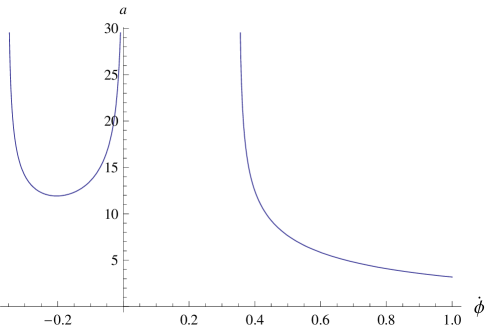
Figure 10: From Eq. (10), the scale factor $a$ as a function of $\dot{\phi}$, when it is consider $\Pi_{\phi}=-113.41$.

References

- (1) A. T. Mithani and A. Vilenkin, JCAP 1201, 028 (2012) [arXiv:1110.4096 [hep-th]].
- (2) A. Mithani and A. Vilenkin, arXiv:1204.4658 [hep-th].
- (3) A. T. Mithani and A. Vilenkin, JCAP 1405, 006 (2014) [arXiv:1403.0818 [hep-th]].
- (4) A. T. Mithani and A. Vilenkin, JCAP 1507, no. 07, 010 (2015) [arXiv:1407.5361 [hep-th]].
- (5) A. Guth, Phys. Rev. D23, 347 (1981); A. Linde, Phys Lett. B 129, 177 (1983); A. Linde; Particle physiscs and inflationary cosmology (Gordon and Breach, New York, 1990).
- (6) D.Larson et al., Astrophys. J. Suppl. textbf192, 16 (2011); Bennett C. et al., Astrophys. J. Suppl. 192, 17 (2011); Hinshaw G. et al. [WMAP Collaboration], Astrophys. J. Suppl. 208, 19 (2013).
- (7) P.A.R. Ade et al. [Planck Collaboration], arXiv:1502.02114 [astro-ph.CO]; P.A.R. Ade et al., Phys. Rev. Lett. 114, 101301 (2015).
- (8) R. Penrose and S. W. Hawking, Proc. R. Soc. A314, 529 (1970); R. P. Geroch, Phys. Rev. Lett. 17, 445 (1966).
- (9) S. W. Hawking and G. F. R. Ellis, The Large Scale Structure of Space-time. Cambridge University Press, New York, 1973.
- (10) A. Borde, A. Vilenkin, Phys.Rev.Lett. 72, 3305 (1994); Int.J.Mod.Phys. D5, 813 (1996).
- (11) G. F.R. Ellis, Roy Maartens, Class.Quant.Grav. 21, 223 (2004); G. F.R. Ellis, J. Murugan, C. G. Tsagas, ibid. 21, 233 (2004).
- (12) D.J. Mulryne, R. Tavakol, J.E. Lidsey and G.F.R. Ellis, Phys. Rev. 71, 123512 (2005); A. Banerjee, T. Bandyopadhyay and S. Chaakraborty, Grav. Cosmol., 290 13 (2007); J.E. Lidsey and D.J. Mulryne Phys. Rev. 73, 083508 (2006); S. Mukherjee, B.C.Paul, S.D. Maharaj and A. Beesham, arXiv:qr-qc/0505103;S. Mukherjee, B.C.Paul, N.K. Dadhich, S.D. Maharaj and A. Beesham, Class.Quant.Grav. 23, 6927 (2006).
- (13) S. del Campo, R. Herrera, P. Labrana, JCAP 0711: 030, (2007); S. del Campo, R. Herrera, P. Labrana, JCAP 0907: 006, (2009).
- (14) S. del Campo, E.I. Guendelman, R. Herrera, P. Labrana,JCAP 1006: 026, (2010).
- (15) S. del Campo, E. Guendelman, A.B. Kaganovich, R. Herrera and P. Labrana, Phys. Lett. B 699, 211 (2011).
- (16) E. I. Guendelman and P. Labrana, Int. J. Mod. Phys. D 22 (2013) 1330018.
- (17) E. Guendelman, R. Herrera, P. Labrana, E. Nissimov and S. Pacheva, Gen. Rel. Grav. 47, no. 2, 10 (2015) [arXiv:1408.5344 [gr-qc]].
- (18) E.I. Guendelman and A.B. Kaganovich, Phys. Rev. D53, 7020 (1996); Mod. Phys. Lett. A12, 2421 (1997); Phys. Rev. D55, 5970 (1997); Mod. Phys. Lett. A12, 2421 (1997); Phys. Rev. D56, 3548 (1997); Mod. Phys. Lett. A13, 1583 (1998).
- (19) E.I. Guendelman and A.B. Kaganovich, Phys. Rev. D60, 065004 (1999).
- (20) E.I. Guendelman, Mod. Phys. Lett. A14, 1043 (1999).
- (21) E.I. Guendelman and O. Katz, Class. Quant. Grav., 20, 1715 (2003).
- (22) E.I. Guendelman, A.B. Kaganovich, Phys.Rev. D75:083505, (2007).
- (23) E.I. Guendelman, A.B. Kaganovich, in Paris 2005, Albert Einstein’s century, p.875, Paris, 2006; hep-th/0603229.
- (24) P. Labrana, Phys. Rev. D 91, no. 8, 083534 (2015) [arXiv:1312.6877 [astro-ph.CO]].
- (25) V. A. Rubakov, Phys. Usp. 57, 128 (2014) doi:10.3367/UFNe.0184.201402b.0137 [arXiv:1401.4024 [hep-th]].
- (26) B.S. DeWitt, Quantum Theory of Gravity. 1. The Canonical Theory, Phys. Rev. 160, 1113 (1967).
- (27) A. Vilenkin, Phys. Rev. D 37, 888 (1988). doi:10.1103/PhysRevD.37.888.
- (28) J. Dittrich and P. Exner, J. Math. Phys. 26, 2000 (1985). J. Dittrich and P. Exner, JINR-E2-84-353. J. Dittrich and P. Exner, JINR-E2-84-352.
- (29) E.I. Guendelman, Class.Quant.Grav. 17, 3673 (2000); E.I. Guendelman, Phys. Rev. D63, 046006 (2002); E.I. Guendelman, A.B. Kaganovich, E. Nissimov, S. Pacheva, Phys. Rev. D66, 046003 (2002); E.I. Guendelman, A. Kaganovich, E. Nissimov, S. Pacheva, Phys.Rev. D72, 086011 (2005).
- (30) P. Labrana, Phys. Rev. D 86, 083524 (2012) doi:10.1103/PhysRevD.86.083524 [arXiv:1111.5360 [gr-qc]]; AIP Conf.Proc. 1606 (2014) 38-47; Astrophys.Space Sci.Proc. 38 (2014) 95-106.