Maximum Likelihood Estimation for Wishart processes

Abstract

In the last decade, there has been a growing interest to use Wishart processes for modelling, especially for financial applications. However, there are still few studies on the estimation of its parameters. Here, we study the Maximum Likelihood Estimator (MLE) in order to estimate the drift parameters of a Wishart process. We obtain precise convergence rates and limits for this estimator in the ergodic case and in some nonergodic cases. We check that the MLE achieves the optimal convergence rate in each case. Motivated by this study, we also present new results on the Laplace transform that extend the recent findings of Gnoatto and Grasselli [17] and are of independent interest.

Keywords : Wishart processes, Laplace transform, parameter inference, maximum likelihood, limit theorems, local asymptotic properties.
AMS MSC 2010: 62F12, 44A10, 60F05, 91B70.

1 Introduction and preliminary results

The goal of this paper is to study the maximum likelihood estimation of the parameters of Wishart processes. These processes have been introduced by Bru [7] and take values in the set of positive semidefinite matrices. Let $d\in\mathbb{N}^{*}$ denote the dimension, $\mathcal{M}_{d}$ be the set of real $d$-square matrices, ${\mathcal{S}_{d}^{+}}$ (resp. ${\mathcal{S}_{d}^{+,*}}$) be the subset of positive semidefinite (resp. definite) matrices, ${\mathcal{S}_{d}}$ (resp. ${\mathcal{A}_{d}}$) the subset of symmetric (resp. antisymmetric) matrices. Wishart processes are defined by the following SDE

$$\left\{\begin{array}[]{ll}dX_{t}=\left[\alpha a^{\top}a+bX_{t}+X_{t}b^{\top}\right]dt+\sqrt{X}_{t}dW_{t}a+a^{\top}dW_{t}^{\top}\sqrt{X}_{t},\quad t>0\\ X_{0}=x\in\textbf{${\mathcal{S}_{d}^{+}}$},\end{array}\right.$$ (3)

where $\alpha\geqslant d-1$, $a\in\mathcal{M}_{d}$, $b\in\mathcal{M}_{d}$ and $(W_{t})_{t\geqslant 0}$ denotes a $d$-square matrix made of independent Brownian motions. We recall that for $x\in\textbf{${\mathcal{S}_{d}^{+}}$}$, $\sqrt{x}$ is the unique matrix in ${\mathcal{S}_{d}^{+}}$ such that $\sqrt{x}^{2}=x$. It is shown by Bru [7] and Cuchiero et al. [8] in a more general affine setting that the SDE (3) has a unique strong solution when $\alpha\geqslant d+1$ and a unique weak solution when $\alpha\geqslant d-1$. Besides, we have $X_{t}\in\textbf{${\mathcal{S}_{d}^{+,*}}$}$ for any $t\geqslant 0$ when $x\in\textbf{${\mathcal{S}_{d}^{+,*}}$}$ and $\alpha\geqslant d+1$. In this paper, we will denote by $WIS_{d}(x,\alpha,b,a)$ the law of $(X_{t},t\geqslant 0)$ and $WIS_{d}(x,\alpha,b,a;t)$ the law of $X_{t}$. In dimension $d=1$, Wishart processes are known as Cox-Ingersoll-Ross processes in the literature. It is worth recalling that the law of $X$ only depends on $a$ through $a^{\top}a$ since we have

$$WIS_{d}(x,\alpha,b,a)\underset{law}{=}WIS_{d}(x,\alpha,b,\sqrt{a^{\top}a}),$$

see e.g. equation (12) in [1]. Therefore, the parameters to estimate are $\alpha$, $b$ and $a^{\top}a$.

Wishart processes have been originally considered by Bru [6] to model some biological data. Recently, they have been widely used in financial models in order to describe the evolution of the dependence between assets. Namely, Gourieroux and Sufana [19] and Da Fonseca et al. [10] have proposed a stochastic volatility model for a basket of assets that assumes that the instantaneous covariance between the assets follows a Wishart process. This extends the well-known Heston model [21] to many assets. Wishart processes have also been used for interest rates models. Affine term structure models involving these processes have been proposed for example by Gourieroux and Sufana [20], Gnoatto [16] and Ahdida et al. [2]. For these models, the question of estimating the parameters of the underlying Wishart process may be important for practical purposes and should be possible thanks to the profusion of financial data. This issue has been considered by Da Fonseca et al. [9] for the model presented in [10]. However, there is no dedicated study on the Maximum Likelihood Estimator (MLE) for Wishart processes. For the Cox-Ingersoll-Ross process, the estimation of parameters has been studied earlier, motivated in particular by its use for interest rates (see Fournié and Talay [14]). Later on, the MLE has been studied by Overbeck [31] including some nonergodic cases, and more recently by Ben Alaya and Kebaier [4, 5]. This paper completes the literature by studying the MLE for Wishart processes.

In this paper, we will follow the theory developed in the books by Lipster and Shiryaev [27] and Kutoyants [23] and assume that we observe the full path $(X_{t},t\in[0,T])$ up to time $T>0$. This choice will be convenient from a mathematical point of view to study the convergence of the MLE. Of course, in practice it can be relevant to study precisely the estimation when we only observe the process on a discrete time-grid. This is left for further research, but we already observe in our numerical experiments that the discrete approximation of the MLE gives a satisfactory estimation of Wishart parameters (see Section 6). It is worth noticing that once we observe the path $(X_{t},t\in[0,T])$, the parameter $a^{\top}a$ is known. In fact, we can calculate the quadratic covariation (see for example Lemma 2 in [1]) and get for $i,j,k,l\in\{1,\cdots,d\}$

$$\langle X_{i,j},X_{k,l}\rangle_{T}= \int_{0}^{T}(a^{\top}a)_{j,l}(X_{s})_{i,k}+(a^{\top}a)_{j,k}(X_{s})_{i,l}+(a^{\top}a)_{i,l}(X_{s})_{j,k}+(a^{\top}a)_{i,k}(X_{s})_{j,l}ds.$$ (4)

This leads to

$$(a^{\top}a)_{i,i} =\frac{1}{4}\langle X_{i,i}\rangle_{T}\Big{(}\int_{0}^{T}(X_{s})_{i,i}ds\Big{)}^{-1},$$ (5)

$$(a^{\top}a)_{i,j} =\left(\frac{1}{2}\langle X_{i,j},X_{i,i}\rangle_{T}-(a^{\top}a)_{i,i}\int_{0}^{T}(X_{s})_{i,j}ds\right)\Big{(}\int_{0}^{T}(X_{s})_{i,i}ds\Big{)}^{-1},$$

for $1\leqslant i,j\leqslant d$ and $j\not=i$. We note that these quantities are well defined as soon as the path $(X_{t},t\in[0,T])$ has a finite quadratic variation and is such that $X_{t}\in\textbf{${\mathcal{S}_{d}^{+,*}}$}$ $dt$-a.e., which is satisfied by the paths of Wishart processes (see Proposition 4 in [7]). We will assume that $a^{\top}a\in\textbf{${\mathcal{S}_{d}^{+,*}}$}$ and denote by $a\in\textbf{${\mathcal{M}_{d}}$}$ an invertible matrix that matches the observed value of $a^{\top}a$: $a$ can be for example the square root of $a^{\top}a$ or the Cholesky decomposition of $a^{\top}a$. Then, we know that $Y_{t}=(a^{\top})^{-1}X_{t}a^{-1}$ follows the law $WIS_{d}((a^{\top})^{-1}xa^{-1},\alpha,(a^{\top})^{-1}ba^{\top},I_{d})$, see e.g. equation (13) in [1]. It is therefore sufficient to focus on the estimation of the parameters $\alpha$ and $b$ when $a=I_{d}$, which we consider now.

We first present the MLE of $\theta=(b,\alpha)$, and we denote by $\mathbb{P}_{\theta}$ the original probability measure under which $X$ satisfies

$$dX_{t}=\left[\alpha I_{d}+bX_{t}+X_{t}b^{\top}\right]dt+\sqrt{X}_{t}dW_{t}+dW_{t}^{\top}\sqrt{X}_{t}.$$ (6)

When no confusion is possible, we also denote $\mathbb{P}$ this probability. We consider $\alpha_{0}\geqslant d+1$ and set $\theta_{0}=(\alpha_{0},0)$. We will assume for the joint estimation of $\alpha$ and $b$ that

$$\alpha\geqslant d+1\text{ and }x\in\textbf{${\mathcal{S}_{d}^{+,*}}$}.$$ (7)

The latter assumption is not restrictive in practice since the condition $\alpha\geqslant d+1$ ensures that $X_{t}\in\textbf{${\mathcal{S}_{d}^{+,*}}$}$ for any $t>0$. Due to this assumption, we know by Theorem 4.1 in Mayerhofer [29] that

$$\frac{d{\mathbb{P}}_{\theta_{0},T}}{d\mathbb{P}_{\theta,T}} :=\exp\left({\int_{0}^{T}\operatorname{Tr}[H_{s}dW_{s}]-\frac{1}{2}\int_{0}^{T}\operatorname{Tr}[H_{s}H_{s}^{\top}]ds}\right),\text{ with }H_{t}=\frac{\alpha_{0}-\alpha}{2}(\sqrt{X_{t}})^{-1}-b\sqrt{X_{t}}$$

defines a probability measure under which $\tilde{W}_{t}=W_{t}-\int_{0}^{t}H^{\top}_{s}ds$ is a $d\times d$-Brownian motion, where $\mathbb{P}_{\theta,T}$ is the restriction of $\mathbb{P}_{\theta}$ to the $\sigma$-algebra $\sigma(W_{s},s\in[0,T])$. We have

$$dX_{t}=\alpha_{0}I_{d}dt+\sqrt{X}_{t}d\tilde{W}_{t}+d\tilde{W}_{t}^{\top}\sqrt{X}_{t},$$

and the likelihood is then defined by (see Lipster and Shiryaev [27], Chapter 7)

$$L_{T}^{\theta,\theta_{0}}=\frac{1}{\mathbb{E}\left[\exp\left({\int_{0}^{T}\operatorname{Tr}[H_{s}dW_{s}]-\frac{1}{2}\int_{0}^{T}\operatorname{Tr}[H_{s}H_{s}^{\top}]ds}\right)\bigg{|}\mathcal{F}^{X}_{T}\right]},$$ (8)

where $(\mathcal{F}^{X}_{t})_{t\geqslant 0}$ denote the filtration generated by the process $X$.

Proposition 1.1.

For $X\in\textbf{${\mathcal{S}_{d}^{+,*}}$}$, let $\mathcal{L}_{X}:\textbf{${\mathcal{S}_{d}}$}\rightarrow\textbf{${\mathcal{S}_{d}}$}$ be the linear application defined by $\mathcal{L}_{X}(Y)=XY+YX$. It is invertible, and the likelihood of $(X_{t},t\in[0,T])$ is given by

$$L_{T}^{\theta,\theta_{0}}=\exp\Bigl{(}\frac{\alpha-\alpha_{0}}{4}\log\left(\frac{\det[X_{T}]}{\det[x]}\right)-\frac{\alpha-\alpha_{0}}{4}\big{(}\frac{\alpha+\alpha_{0}}{2}-1-d\big{)}\int_{0}^{T}\operatorname{Tr}[X_{s}^{-1}]ds-\frac{\alpha T}{2}\operatorname{Tr}[b]\\ +\frac{1}{2}\int_{0}^{T}\operatorname{Tr}\left[\mathcal{L}_{X_{t}}^{-1}\left(bX_{t}+X_{t}b^{\top}\right)dX_{t}\right]-\frac{1}{4}\int_{0}^{T}\operatorname{Tr}\left[\mathcal{L}_{X_{t}}^{-1}\left(bX_{t}+X_{t}b^{\top}\right)(bX_{t}+X_{t}b^{\top})\right]dt\Bigr{)}.$$ (9)

Lemmas B.1 and B.2 states some properties of $\mathcal{L}_{X}$, and the proof of Proposition 1.1 is given in Appendix A. In particular, we see from this proof that $\frac{d{\mathbb{P}}_{\theta_{0},T}}{d\mathbb{P}_{\theta,T}}\in\mathcal{F}^{X}_{T}$ if, and only if $b\in\textbf{${\mathcal{S}_{d}}$}$, in which case the likelihood has the following simpler form

$$L_{T}^{\theta,\theta_{0}}=\exp\Bigl{(}\frac{\alpha-\alpha_{0}}{4}\log\left(\frac{\det[X_{T}]}{\det[x]}\right)+\frac{\operatorname{Tr}[bX_{T}]-{\operatorname{Tr}[bx]}}{2}-\frac{1}{2}\int_{0}^{T}\operatorname{Tr}[b^{2}X_{s}]ds\\ -\frac{\alpha-\alpha_{0}}{4}\big{(}\frac{\alpha+\alpha_{0}}{2}-1-d\big{)}\int_{0}^{T}\operatorname{Tr}[X_{s}^{-1}]ds-\frac{\alpha T}{2}\operatorname{Tr}[b]\Bigr{)},$$ (10)

since $\mathcal{L}_{X_{t}}^{-1}\left(bX_{t}+X_{t}b\right)=b$.

Now, we want to maximize the likelihood and observe that the quantity in the exponential (9) is quadratic with respect to $(b,\alpha)$ and goes almost surely to $-\infty$ when $\|(b,\alpha)\|\rightarrow+\infty$. To do so, we first remark that $\operatorname{Tr}[b]=\operatorname{Tr}[\mathcal{L}_{X_{t}}^{-1}\left(bX_{t}+X_{t}b^{\top}\right)]$ by Lemma B.1. Then, Cauchy-Schwarz inequality yields to

$$|\operatorname{Tr}[\alpha b]| =\left|\frac{1}{T}\int_{0}^{T}\operatorname{Tr}\left[\sqrt{2}\mathcal{L}_{X_{s}}^{-1}\left(bX_{s}+X_{s}b^{\top}\right)\sqrt{X_{s}}\frac{\alpha}{\sqrt{2}}\sqrt{X_{s}^{-1}}\right]ds\right|$$

$$\leqslant\frac{1}{T}\int_{0}^{T}\operatorname{Tr}\left[(\mathcal{L}_{X_{s}}^{-1}\left(bX_{s}+X_{s}b^{\top}\right))^{2}X_{s}\right]ds+\frac{\alpha^{2}}{4}\frac{1}{T}\int_{0}^{T}\operatorname{Tr}\left[X_{s}^{-1}\right]ds$$ (11)

$$=\frac{1}{2T}\int_{0}^{T}\operatorname{Tr}\left[\mathcal{L}_{X_{s}}^{-1}\left(bX_{s}+X_{s}b^{\top}\right)(bX_{s}+X_{s}b^{\top})\right]ds+\frac{\alpha^{2}}{4}\frac{1}{T}\int_{0}^{T}\operatorname{Tr}\left[X_{s}^{-1}\right]ds,$$

and it is strict almost surely, which gives that the quadratic form in the exponential (9) is negative definite. There is thus a unique global maximum of (9) on $\mathbb{R}\times\textbf{${\mathcal{M}_{d}}$}$. We know from Lemma B.2 that $\mathcal{L}_{X_{s}}^{-1}$ is self-adjoint, and we get with straightforward calculations that the MLE $\hat{\theta}_{T}=(\hat{b}_{T},\hat{\alpha}_{T})$ is characterized by the following equations:

$$\begin{cases}\frac{1}{4}\log\left(\frac{\det[X_{T}]}{\det[x]}\right)-\frac{\hat{\alpha}_{T}-1-d}{4}\int_{0}^{T}\operatorname{Tr}[X_{s}^{-1}]ds-\frac{T}{2}\operatorname{Tr}[\hat{b}_{T}]=0,\\ \int_{0}^{T}\mathcal{L}_{X_{s}}^{-1}(dX_{s})X_{s}-\int_{0}^{T}\mathcal{L}_{X_{s}}^{-1}(\hat{b}_{T}X_{s}+X_{s}\hat{b}_{T}^{\top})X_{s}ds-\frac{\hat{\alpha}_{T}T}{2}I_{d}=0.\end{cases}$$ (12)

Unless in the ergodic case, we will not be able to obtain convergence results for this estimator. Instead, we will mostly work with the MLE estimator when $b$ is known to be symmetric. This enables us to work with more tractable formulas, even if the calculations are already quite involved in case. Analyzing the general case would require development of further arguments. Besides, we can consider that Wishart processes with $b$ symmetric already form an interesting family of processes that may be rich enough in many applications. When $b\in\textbf{${\mathcal{S}_{d}}$}$, the unique global maximum $\hat{\theta}_{T}=(\hat{b}_{T},\hat{\alpha}_{T})$ of (10) on $\mathbb{R}\times\textbf{${\mathcal{S}_{d}}$}$ is characterized by the following equations:

$$\begin{cases}\frac{1}{4}\log\left(\frac{\det[X_{T}]}{\det[x]}\right)-\frac{\hat{\alpha}_{T}-1-d}{4}\int_{0}^{T}\operatorname{Tr}[X_{s}^{-1}]ds-\frac{T}{2}\operatorname{Tr}[\hat{b}_{T}]=0,\\ \frac{X_{T}-{x}}{2}-\frac{1}{2}\int_{0}^{T}(\hat{b}_{T}X_{s}+X_{s}\hat{b}_{T})ds-\frac{\hat{\alpha}_{T}T}{2}I_{d}=0.\end{cases}$$ (13)

To get more explicit formulas, we have to invert this linear system. For $X\in\textbf{${\mathcal{S}_{d}}$}$ and $a\in\mathbb{R}$, we define the linear applications

$$\mathcal{L}_{X}:\begin{array}[t]{l}\textbf{${\mathcal{S}_{d}}$}\rightarrow\textbf{${\mathcal{S}_{d}}$}\\ Y\mapsto YX+XY\end{array}\text{ and }\mathcal{L}_{X,a}:\begin{array}[t]{l}\textbf{${\mathcal{S}_{d}}$}\rightarrow\textbf{${\mathcal{S}_{d}}$}\\ Y\mapsto YX+XY-2a\operatorname{Tr}[Y]I_{d}.\end{array}$$ (18)

We introduce the following shorthand notation

$$R_{T}:=\int_{0}^{T}X_{s}ds,\quad Q_{T}:=\left(\int_{0}^{T}\operatorname{Tr}[X_{s}^{-1}]ds\right)^{-1},\quad Z_{T}:=\log\left(\dfrac{\det[X_{T}]}{\det[x]}\right),$$ (19)

and note that $Q_{T}$ and $Z_{T}$ are defined only for $\alpha\geqslant d+1$ while $R_{T}$ is defined for $\alpha\geqslant d-1$ and belongs almost surely to ${\mathcal{S}_{d}^{+,*}}$. By using the convexity property of the inverse, see e.g. Mond and Pecaric [30], we have when $\alpha\geqslant d+1$

$$\operatorname{Tr}\left[\left(\frac{R_{T}}{T}\right)^{-1}\right]<\frac{Q_{T}^{-1}}{T},\ a.s.$$ (20)

We get $\hat{\alpha}_{T}=1+d+Q_{T}\big{(}Z_{T}-2T\operatorname{Tr}[\hat{b}_{T}]\big{)}$ and $\mathcal{L}_{R_{T},T^{2}Q_{T}}(\hat{b}_{T})=X_{T}-{x}-T\left(Q_{T}Z_{T}+1+d\right)I_{d}$. By (20) and Lemma B.1, the latter equation can be inverted, which leads to

$$\left\{\begin{array}[]{l l l}\hat{\alpha}_{T}&=&1+d+Q_{T}\Big{(}Z_{T}-2T\operatorname{Tr}\big{[}\mathcal{L}^{-1}_{R_{T},T^{2}Q_{T}}\left({X_{T}-{x}}-T\left[Q_{T}Z_{T}+1+d\right]I_{d}\right)\big{]}\Big{)}\\ \\ \hat{b}_{T}&=&\mathcal{L}^{-1}_{R_{T},T^{2}Q_{T}}\left({X_{T}-{x}}-T\left[Q_{T}Z_{T}+1+d\right]I_{d}\right).\end{array}\right.$$ (24)

The estimator of $\alpha$ when $\alpha\in[d-1,d+1)$ given by the MLE is no longer well defined. The same thing already occurs in dimension $d=1$ for the CIR process, see Ben Alaya and Kebaier [4]. However, it is still possible to estimate the parameter $b\in\textbf{${\mathcal{M}_{d}}$}$ when $\alpha\geqslant d-1$ is known. In this case, we denote $\theta=(b,\alpha)$ and $\theta_{0}=(0,\alpha)$ and get by repeating the same arguments that

$$L_{T}^{\theta,\theta_{0}}=\exp\Bigl{(}\frac{1}{2}\int_{0}^{T}\operatorname{Tr}\left[\mathcal{L}_{X_{t}}^{-1}\left(bX_{t}+X_{t}b^{\top}\right)dX_{t}\right]\\ -\frac{1}{4}\int_{0}^{T}\operatorname{Tr}\left[\mathcal{L}_{X_{t}}^{-1}\left(bX_{t}+X_{t}b^{\top}\right)(bX_{t}+X_{t}b^{\top})\right]dt-\frac{\alpha T}{2}\operatorname{Tr}[b]\Bigr{)},$$

and the MLE is characterized by

$$\int_{0}^{T}\mathcal{L}_{X_{s}}^{-1}(dX_{s})X_{s}-\int_{0}^{T}\mathcal{L}_{X_{s}}^{-1}(\hat{b}_{T}X_{s}+X_{s}\hat{b}_{T}^{\top})X_{s}ds-\frac{\alpha T}{2}I_{d}=0.$$ (25)

When $b$ is known a priori to be symmetric, the likelihood and the MLE are then given by

$$L_{T}^{\theta,\theta_{0}} =\exp\Bigl{(}\frac{\operatorname{Tr}[bX_{T}]-{\operatorname{Tr}[bx]}}{2}-\frac{1}{2}\int_{0}^{T}\operatorname{Tr}[b^{2}X_{s}]ds-\frac{\alpha T}{2}\operatorname{Tr}[b]\Bigr{)},$$ (26)

$$\hat{b}_{T} =\mathcal{L}^{-1}_{R_{T}}\left(X_{T}-x-\alpha TI_{d}\right).$$ (27)

The goal of the paper is to study the convergence of the MLE under the original probability $\mathbb{P}_{\theta}$. To do so, we first consider the case where the Wishart process is ergodic. By Lemma C.1, this holds if $-(b+b^{\top})\in\textbf{${\mathcal{S}_{d}^{+,*}}$}$ when $b\in\textbf{${\mathcal{M}_{d}}$}$, and the ergodicity is equivalent to $-b\in\textbf{${\mathcal{S}_{d}^{+,*}}$}$ when $b\in\textbf{${\mathcal{S}_{d}}$}$. Then, we can use Birkhoff’s ergodic theorem to determine the convergence of the MLE. Section 2 presents these results for (24) when $\alpha\geqslant d+1$, for (9) when $\alpha>d+1$ and for both (27) and (25) when $\alpha\geqslant d-1$. Section 3 studies the convergence of the MLE in some nonergodic cases, namely when $b=\lambda_{0}I_{d}$ with $\lambda_{0}\geqslant 0$ and when $b$ is known to be symmetric. More precisely, when $b=0$, we obtain convergence results for (24) when $\alpha\geqslant d+1$ and for (27) when $\alpha\geqslant d-1$. When $\lambda_{0}>0$, we only obtain convergence results for (27) when $\alpha\geqslant d-1$. In all these cases, we analyse the convergence by the mean of Laplace transforms. Though limited to some nonergodic cases, we however recover and extend the recent convergence results obtained by Ben Alaya and Kebaier for the one-dimensional CIR process [4, 5]. In Section 4, we check that the MLE achieves the optimal rate of convergence in the different cases by proving local asymptotic properties. Last, we study in Section 5 the Laplace transform of $(X_{T},R_{T})$. This study can be of independent interest and improves the recent results of Gnoatto and Grasselli [17].

2 Statistical Inference of the Wishart process: the ergodic case

When $-(b+b^{\top})\in\textbf{${\mathcal{S}_{d}^{+,*}}$}$, the Wishart process $X_{t}$ converges in law when $t\rightarrow+\infty$ to the stationary law $X_{\infty}\sim WIS_{d}(0,\alpha,0,\sqrt{2q_{\infty}};1/2)$ with $q_{\infty}=\int_{0}^{\infty}e^{sb}e^{sb^{\top}}ds$ for any starting point $x\in\textbf{${\mathcal{S}_{d}^{+}}$}$ by Lemma C.1. Therefore this is the unique stationary law which is thus extremal, and we know by Stroock ([35], Theorem 7.4.8) that it is then ergodic, see also Pagès [32], Annex A. We introduce the following quantity

$$\overline{R}_{\infty}:=\mathbb{E}_{\theta}(X_{\infty}).$$

From the ergodic Birkhoff’s theorem, we have

$$\frac{R_{T}}{T}\overset{a.s.}{\longrightarrow}\overline{R}_{\infty},\quad\mbox{ as }T\rightarrow+\infty.$$ (28)

Besides, when $\alpha\geqslant d+1$, $\overline{Q}_{\infty}=\frac{1}{\mathbb{E}_{\theta}(\operatorname{Tr}[X_{\infty}^{-1}])}$ is finite and satisfies

$$\overline{Q}_{\infty}\operatorname{Tr}[\overline{R}_{\infty}^{-1}]<1,$$ (29)

due to the convexity property of the inverse, see e.g. Mond and Pecaric [30]. Again, the ergodic Birkhoff’s theorem gives

$$TQ_{T}\overset{a.s.}{\longrightarrow}\overline{Q}_{\infty}=\frac{1}{\mathbb{E}_{\theta}(\operatorname{Tr}[X_{\infty}^{-1}])},\quad\mbox{ as }T\rightarrow+\infty.$$ (30)

This section is organized as follows. First, we study the MLE (24) when $b$ is known to be symmetric in the cases $\alpha>d+1$ and $\alpha=d+1$. Then, we focus on the MLE (12) when $b\in\textbf{${\mathcal{M}_{d}}$}$ and $\alpha>d+1$. The analysis follows the same steps and reuses some calculations made in the symmetric case. Last, we study the convergence of the MLE when $\alpha\geqslant d-1$ is known, in both symmetric and general cases.

2.1 The global MLE estimator of $\theta=(b,\alpha)$ when $b$ is known to be symmetric

When $b\in\textbf{${\mathcal{S}_{d}}$}$, the ergodicity is by Lemma (C.1) equivalent to $-b\in\textbf{${\mathcal{S}_{d}^{+,*}}$}$, which we assume in this subsection. We have $X_{\infty}\sim WIS_{d}(0,\alpha,0,\sqrt{-b^{-1}};1/2)$ and it is easy to get from (6) that $\alpha I_{d}+b\overline{R}_{\infty}+\overline{R}_{\infty}b=0$, which gives $\overline{R}_{\infty}=-\frac{\alpha}{2}b^{-1}\in\textbf{${\mathcal{S}_{d}^{+,*}}$}$. We will also show in the proof of Theorem 2.1 that

$$\overline{Q}_{\infty}:=\frac{\alpha-(1+d)}{2\operatorname{Tr}[-b]}.$$ (31)

We consider the convergence of the MLE given by (24) when $\alpha\geqslant d+1$. We introduce the following martingales:

$$M_{t} :=\int_{0}^{t}\sqrt{X_{s}}d{W}_{s}+\int_{0}^{t}d{W}^{\top}_{s}\sqrt{X}_{s},$$ (32)

$$N_{t} :=\int_{0}^{t}\operatorname{Tr}[(\sqrt{X_{s}})^{-1}d{W}_{s}].$$ (33)

We use the dynamics of $(X_{t})_{t\geqslant 0}$ under ${\mathbb{P}}_{\theta}$ and Itô’s formula for $(Z_{t})_{t\geqslant 0}$ (see e.g. Bru [7], equation (2.6)) to get on the one hand

$$X_{T} =x+\alpha TI_{d}+\mathcal{L}_{R_{T}}(b)+M_{T}, Z_{T} =(\alpha-1-d)Q_{T}^{-1}+2\operatorname{Tr}[b]T+2N_{T}.$$ (34)

On the other hand, we obtain from (13) and (19) that $X_{T}=x+\hat{\alpha}_{T}TI_{d}+\mathcal{L}_{R_{T}}(\hat{b}_{T})$ and $Z_{T}=(\hat{\alpha}_{T}-1-d)Q_{T}^{-1}+2T\operatorname{Tr}[\hat{b}_{T}]$, which yields to

$$\left\{\begin{array}[]{r c l}\hat{\alpha}_{T}-\alpha&=&2TQ_{T}\operatorname{Tr}[b-\hat{b}_{T}]+2Q_{T}N_{T}\\ \\ \mathcal{L}_{R_{T}}(\hat{b}_{T}-b)&=&(\alpha-\hat{\alpha}_{T})TI_{d}+M_{T}=2T^{2}Q_{T}\operatorname{Tr}[\hat{b}_{T}-b]I_{d}+M_{T}-2TQ_{T}N_{T}I_{d}.\end{array}\right.$$ (35)

Theorem 2.1.

Assume that $-b\in S^{+,*}_{d}$ and $\alpha>d+1$. Under $\mathbb{P}_{\theta}$, $\left(\sqrt{T}(\hat{b}_{T}-b,\hat{\alpha}_{T}-\alpha)\right)$ converges in law when $T\rightarrow+\infty$ to the centered Gaussian vector $(\mathbf{G},H)$ that takes values in $\textbf{${\mathcal{S}_{d}}$}\times\mathbb{R}$ and has the following Laplace transform: for $c,\lambda\in\textbf{${\mathcal{S}_{d}}$}\times\mathbb{R}$,

$$\mathbb{E}_{\theta}\left[\exp\left(\operatorname{Tr}[c\mathbf{G}]+\lambda H\right)\right]=\exp\left(\frac{2\overline{Q}_{\infty}\lambda^{2}}{1-\overline{Q}_{\infty}\operatorname{Tr}[\overline{R}_{\infty}^{-1}]}-\frac{2\overline{Q}_{\infty}\lambda}{1-\overline{Q}_{\infty}\operatorname{Tr}[\overline{R}_{\infty}^{-1}]}\operatorname{Tr}[c\overline{R}_{\infty}^{-1}]+\operatorname{Tr}[c\mathcal{L}^{-1}_{\overline{R}_{\infty},\overline{Q}_{\infty}}(c)]\right).$$

Proof.

By (20) and Lemma B.1, we can rewrite the system (35) as follows

$$\left\{\begin{array}[]{r c l}\sqrt{T}(\hat{\alpha}_{T}-\alpha)&=&2TQ_{T}\dfrac{N_{T}}{\sqrt{T}}-2TQ_{T}\operatorname{Tr}\left[\mathcal{L}^{-1}_{\frac{R_{T}}{T},TQ_{T}}\left(\dfrac{M_{T}}{\sqrt{T}}-2TQ_{T}I_{d}\dfrac{N_{T}}{\sqrt{T}}\right)\right]\\ \\ \sqrt{T}(\hat{b}_{T}-b)&=&\mathcal{L}^{-1}_{\frac{R_{T}}{T},TQ_{T}}\left(\dfrac{M_{T}}{\sqrt{T}}-2TQ_{T}I_{d}\dfrac{N_{T}}{\sqrt{T}}\right).\end{array}\right.$$

Note that, for $i,j,k,l\in\{1,\dots,d\}$ we have

$$\langle M_{i,j},M_{k,l}\rangle_{t} = \left[\delta_{jl}(R_{t})_{i,k}+\delta_{jk}(R_{t})_{i,l}+\delta_{il}(R_{t})_{j,k}+\delta_{ik}(R_{t})_{j,l}\right],$$

$$\langle M_{i,j},N\rangle_{t} = 2t\delta_{ij}\quad\mbox{ and }\quad\langle N\rangle_{t}=Q_{t}^{-1},$$ (36)

where $\delta_{ij}$ stands for the Kronecker symbol.

So, it follows from the central limit theorem for martingales (see e.g., Kutoyants [23], Proposition 1.21), that $(\frac{M_{T}}{\sqrt{T}},\frac{N_{T}}{\sqrt{T}})$ converges in law under $\mathbb{P}_{\theta}$ towards a centered Gaussian vector $(\tilde{\mathbf{G}},\tilde{H})$ taking values in $\textbf{${\mathcal{S}_{d}}$}\times\mathbb{R}$ such that

$$\mathbb{E}_{\theta}(\tilde{\mathbf{G}}_{i,j}\tilde{\mathbf{G}}_{k,l}) =\left[\delta_{jl}(\overline{R}_{\infty})_{i,k}+\delta_{jk}(\overline{R}_{\infty})_{i,l}+\delta_{il}(\overline{R}_{\infty})_{j,k}+\delta_{ik}(\overline{R}_{\infty})_{j,l}\right],$$ (37)

$$\mathbb{E}_{\theta}(\tilde{\mathbf{G}}_{i,j}\tilde{H}) =2\delta_{i,j}\text{ and }\mathbb{E}_{\theta}(\tilde{H}^{2})=\overline{Q}_{\infty}^{-1}.$$

From (34) and (30), we obtain (31). From Lemma B.1, the function $(X,Y,a)\mapsto\mathcal{L}^{-1}_{X,a}(Y)$ is continuous, and we get by Slutsky’s theorem that $(\sqrt{T}(\hat{b}_{T}-b),\sqrt{T}(\hat{\alpha}_{T}-\alpha))$ converges in law to the Gaussian vector

$$(\mathbf{G},H)=\left(\mathcal{L}^{-1}_{\overline{R}_{\infty},\overline{Q}_{\infty}}\left(\tilde{\mathbf{G}}-2\overline{Q}_{\infty}\tilde{H}I_{d}\right),2\overline{Q}_{\infty}\left(\tilde{H}-\operatorname{Tr}\left[\mathcal{L}^{-1}_{\overline{R}_{\infty},\overline{Q}_{\infty}}\left(\tilde{\mathbf{G}}-2\overline{Q}_{\infty}\tilde{H}I_{d}\right)\right]\right)\right).$$

We are interested to calculate the Laplace transform of this law. First, we calculate the Laplace transform of $(\tilde{\mathbf{G}},\tilde{H})$:

$$\forall c\in\textbf{${\mathcal{S}_{d}}$},\lambda\in\mathbb{R},\mathbb{E}_{\theta}\left[\exp\left(\operatorname{Tr}[c\tilde{\mathbf{G}}]+\lambda\tilde{H}\right)\right]=\exp\left(\frac{1}{2}\left(\lambda^{2}\overline{Q}_{\infty}^{-1}+4\lambda\operatorname{Tr}[c]+4\operatorname{Tr}[c^{2}\overline{R}_{\infty}]\right)\right).$$ (38)

We want to calculate for $c\in\textbf{${\mathcal{S}_{d}}$}$ and $\lambda\in\mathbb{R}$,

$$\mathbb{E}_{\theta}\left[\exp\left(\operatorname{Tr}[c\mathbf{G}]+\lambda H\right)\right] =\mathbb{E}_{\theta}\left[\exp\left(\operatorname{Tr}[(c-2\lambda\overline{Q}_{\infty}I_{d}){\mathbf{G}}]+2\lambda\overline{Q}_{\infty}\tilde{H}\right)\right].$$

Due to (29) and Lemma B.1, we can introduce $\tilde{c}=\mathcal{L}^{-1}_{\overline{R}_{\infty},\overline{Q}_{\infty}}(c-2\lambda\overline{Q}_{\infty}I_{d})$. We have

$$\overline{R}_{\infty}\tilde{c}+\tilde{c}\overline{R}_{\infty}-2\overline{Q}_{\infty}\operatorname{Tr}[\tilde{c}]I_{d}=c-2\lambda\overline{Q}_{\infty}I_{d},$$

and thus

$$\operatorname{Tr}[(c-2\lambda\overline{Q}_{\infty}I_{d})\mathbf{G}] =\operatorname{Tr}[(\overline{R}_{\infty}\tilde{c}+\tilde{c}\overline{R}_{\infty}-2\overline{Q}_{\infty}\operatorname{Tr}[\tilde{c}]I_{d})\mathbf{G}]$$

$$=\operatorname{Tr}[\tilde{c}(\overline{R}_{\infty}\mathbf{G}+\mathbf{G}\overline{R}_{\infty}-2\overline{Q}_{\infty}\operatorname{Tr}[\mathbf{G}]I_{d})]=\operatorname{Tr}[\tilde{c}(\tilde{\mathbf{G}}-2\overline{Q}_{\infty}\tilde{H}I_{d})].$$

We therefore obtain from (38)

$$\mathbb{E}_{\theta}\left[\exp\left(\operatorname{Tr}[c\mathbf{G}]+\lambda H\right)\right]$$

$$=\mathbb{E}_{\theta}\left[\exp\left(\operatorname{Tr}[\tilde{c}(\tilde{\mathbf{G}}-2\overline{Q}_{\infty}\tilde{H}I_{d})]+2\lambda\overline{Q}_{\infty}\tilde{H}\right)\right]$$

$$=\mathbb{E}_{\theta}\left[\exp\left(\operatorname{Tr}[\tilde{c}\tilde{\mathbf{G}}]+2\overline{Q}_{\infty}(\lambda-\operatorname{Tr}[\tilde{c}])\tilde{H}\right)\right]$$

$$=\exp\left(2\left\{(\lambda-\operatorname{Tr}[\tilde{c}])^{2}\overline{Q}_{\infty}+2(\lambda-\operatorname{Tr}[\tilde{c}])\operatorname{Tr}[\tilde{c}]\overline{Q}_{\infty}+\operatorname{Tr}[\tilde{c}^{2}\overline{R}_{\infty}]\right\}\right).$$

Since $2\operatorname{Tr}[\tilde{c}^{2}\overline{R}_{\infty}]=\operatorname{Tr}[\tilde{c}(\tilde{c}\overline{R}_{\infty}+\overline{R}_{\infty}\tilde{c})]=\operatorname{Tr}[\tilde{c}c]+2\overline{Q}_{\infty}(\operatorname{Tr}[\tilde{c}]-\lambda)\operatorname{Tr}[\tilde{c}]$, we get

$$\mathbb{E}_{\theta}\left[\exp\left(\operatorname{Tr}[c\mathbf{G}]+\lambda H\right)\right]=\exp\left(2\lambda(\lambda-\operatorname{Tr}[\tilde{c}])\overline{Q}_{\infty}+\operatorname{Tr}[\tilde{c}c]\right).$$

We now use that $\mathcal{L}^{-1}_{\overline{R}_{\infty},\overline{Q}_{\infty}}(I_{d})=\frac{1}{2(1-\overline{Q}_{\infty}\operatorname{Tr}[\overline{R}_{\infty}^{-1}])}\overline{R}_{\infty}^{-1}$ to get $\tilde{c}=\mathcal{L}^{-1}_{\overline{R}_{\infty},\overline{Q}_{\infty}}(c)-\lambda\frac{\overline{Q}_{\infty}\overline{R}_{\infty}^{-1}}{1-\overline{Q}_{\infty}\operatorname{Tr}[\overline{R}_{\infty}^{-1}]}$. Since we have $\operatorname{Tr}[\mathcal{L}^{-1}_{\overline{R}_{\infty},\overline{Q}_{\infty}}(c)]=\frac{\operatorname{Tr}[\overline{R}_{\infty}^{-1}c]}{2(1-\overline{Q}_{\infty}\operatorname{Tr}[\overline{R}_{\infty}^{-1}])}$ by Lemma B.1, this yields to the claimed result. ∎

When $\alpha=d+1$, the rate of convergence of the MLE of $\alpha$ is even better as stated by the following theorem.

Theorem 2.2.

Assume $-b\in S^{+,*}_{d}$ and $\alpha=d+1$. Then, under $\mathbb{P}_{\theta}$, $\left(\sqrt{T}(\hat{b}_{T}-b),T(\hat{\alpha}_{T}-\alpha)\right)$ converges in law when $T\rightarrow+\infty$ to $\left(\mathbf{G},-2\tau^{-1}_{{}_{-\operatorname{Tr}[b]}}\operatorname{Tr}[b]\right)$, where $\tau_{a}=\inf\{t\geq 0,\;B_{t}=a\}$ with $(B_{t})_{t\geq 0}$ a given one-dimensional standard Brownian motion and $\mathbf{G}$ is a Gaussian vector independent of $B$ such that $\mathbb{E}_{\theta}\left[\exp\left(\operatorname{Tr}[c\mathbf{G}]\right)\right]=\exp\left(\operatorname{Tr}[c\mathcal{L}^{-1}_{\overline{R}_{\infty}}(c)]\right)$, $c\in\textbf{${\mathcal{S}_{d}}$}$.

Proof.

By (20) and Lemma B.1, we can rewrite the system (35) as follows

$$\left\{\begin{array}[]{r c l}T(\hat{\alpha}_{T}-\alpha)&=&2T^{2}Q_{T}\left(\dfrac{N_{T}}{T}-\frac{1}{\sqrt{T}}\operatorname{Tr}\left[\mathcal{L}^{-1}_{\frac{R_{T}}{T},TQ_{T}}\left(\dfrac{M_{T}}{\sqrt{T}}-2T^{3/2}Q_{T}I_{d}\dfrac{N_{T}}{T}\right)\right]\right)\\ \\ \sqrt{T}(\hat{b}_{T}-b)&=&\mathcal{L}^{-1}_{\frac{R_{T}}{T},TQ_{T}}\left(\dfrac{M_{T}}{\sqrt{T}}-2T^{3/2}Q_{T}I_{d}\dfrac{N_{T}}{T}\right).\end{array}\right.$$ (39)

From (34), we have

$$\frac{N_{T}}{T}=\frac{1}{2T}\log\left(\dfrac{\det[X_{T}]}{\det[x]}\right)-\operatorname{Tr}[b].$$

As for $-b\in S^{+,*}_{d}$ the Wishart process $(X_{t})_{t\geq 0}$ is stationary with invariant limit distribution $X_{\infty}$ we easily deduce that $\frac{N_{T}}{T}$ converges in probability to $-\operatorname{Tr}[b]$ when $T\rightarrow\infty$. Then, it follows from (28) that

$$(T^{-1}R_{T},T^{-1}N_{T})\overset{\mathbb{P}_{\theta}}{\rightarrow}(\overline{R}_{\infty},-\operatorname{Tr}[b]),\quad{as}\;T\rightarrow\infty.$$ (40)

Hence, we only need to study the asymptotic behavior of the couple $(T^{-1/2}M_{T},T^{2}Q_{T})$. According to Theorem 4.1 in Mayerhofer [29], we have for $\lambda\geqslant 0$ and $\Gamma\in S_{d}$

$$\mathbb{E}_{\theta}\left[\exp\left(\frac{\lambda}{T}N_{T}-\frac{\lambda^{2}}{2T^{2}}Q_{T}^{-1}+\frac{1}{\sqrt{T}}\operatorname{Tr}[\Gamma M_{T}]-\frac{2}{T}\int_{0}^{T}\operatorname{Tr}[\Gamma^{2}X_{s}]ds-\frac{2\lambda}{\sqrt{T}}\operatorname{Tr}[\Gamma]\right)\right]=1.$$ (41)

Now, let us introduce the quantity

$$A_{T}=\mathbb{E}_{\theta}\left[\exp\left(\lambda\frac{N_{T}}{T}+\lambda\operatorname{Tr}[b]\right)\exp\left(-\frac{\lambda^{2}}{2T^{2}}Q_{T}^{-1}+\frac{1}{\sqrt{T}}\operatorname{Tr}[\Gamma M_{T}]\right)\right.\\ \times\left.\exp\left(-\frac{2}{T}\int_{0}^{T}\operatorname{Tr}[\Gamma^{2}X_{s}]ds+2\operatorname{Tr}[\Gamma^{2}\overline{R}_{\infty}]\right)\right].$$

Then, by (41) we easily get $A_{T}=\exp\left(\lambda\operatorname{Tr}[b]+2\operatorname{Tr}[\Gamma^{2}\overline{R}_{\infty}]+\frac{2\lambda}{\sqrt{T}}\operatorname{Tr}[\Gamma]\right).$ We now write $A_{T}=\tilde{A}_{T}+\mathbb{E}_{\theta}\left[\exp\left(-\frac{\lambda^{2}}{2T^{2}}Q_{T}^{-1}+\frac{1}{\sqrt{T}}\operatorname{Tr}[\Gamma M_{T}]\right)\right]$ with

$$\tilde{A}_{T} =\mathbb{E}_{\theta}\left[(\exp\left(\xi_{T}\right)-1)\exp\left(-\frac{\lambda^{2}}{2T^{2}}Q_{T}^{-1}+\frac{1}{\sqrt{T}}\operatorname{Tr}[\Gamma M_{T}]\right)\right]$$

$$\xi_{T} =\lambda\frac{N_{T}}{T}+\lambda\operatorname{Tr}[b]-\frac{2}{T}\int_{0}^{T}\operatorname{Tr}[\Gamma^{2}X_{s}]ds+2\operatorname{Tr}[\Gamma^{2}\overline{R}_{\infty}].$$

Cauchy-Schwarz inequality and $Q_{T}^{-1}>0$ give

$$|\tilde{A}_{T}|\leqslant\mathbb{E}_{\theta}^{1/2}[\exp\left(2\xi_{T}\right)-2\exp\left(\xi_{T}\right)+1]\mathbb{E}_{\theta}^{1/2}\left[\exp\left(\frac{2}{\sqrt{T}}\operatorname{Tr}[\Gamma M_{T}]\right)\right].$$

On the one hand, Proposition 5.1 with $m=-b\in\textbf{${\mathcal{S}_{d}^{+,*}}$}$ gives

$$\mathbb{E}_{\theta}\left[\exp\left(\frac{2}{\sqrt{T}}\operatorname{Tr}[\Gamma M_{T}]\right)\right]\leqslant\mathbb{E}_{\theta}\left[\exp\left(\frac{2}{T}\operatorname{Tr}[\Gamma^{2}R_{T}]\right)\right]<\infty.$$

On the other hand, we have for any $r\geqslant 0$,

$$\mathbb{E}_{\theta}[\exp\left(r\xi_{T}\right)]\leqslant\mathbb{E}_{\theta}\left[\exp\left(\frac{\lambda r}{T}N_{T}\right)\right]\exp(2r\operatorname{Tr}[\Gamma^{2}\overline{R}_{\infty}]).$$

From (34), we have

$$\mathbb{E}_{\theta}\left[\exp\left(\frac{\lambda r}{T}N_{T}\right)\right]=\exp(-\lambda r\operatorname{Tr}[b])\mathbb{E}_{\theta}\left[\left(\frac{\det[X_{T}]}{\det[x]}\right)^{\frac{\lambda r}{2T}}\right].$$

The sublinear growth of the coefficients of the Wishart SDE and the convergence to a stationary law gives that $\mathbb{E}_{\theta}\left[\left(\frac{\det[X_{T}]}{\det[x]}\right)^{\tilde{\lambda}}\right]$ is uniformly bounded in $T>0,\ \tilde{\lambda}<1$ and therefore $\sup_{T>\frac{\lambda r}{2}}\mathbb{E}_{\theta}\left[\left(\frac{\det[X_{T}]}{\det[x]}\right)^{\frac{\lambda r}{2T}}\right]<\infty$. This gives the uniform integrability of the family $(\exp\left(2\xi_{T}\right),T>\lambda)$. Then, we deduce from (40) that $\mathbb{E}_{\theta}[\exp\left(2\xi_{T}\right)-2\exp\left(\xi_{T}\right)+1]\underset{T\rightarrow+\infty}{\rightarrow}0$ and thus $\tilde{A}_{T}\underset{T\rightarrow+\infty}{\rightarrow}0$.

Hence, we obtain

$$\lim_{T\rightarrow\infty}\mathbb{E}_{\theta}\left[\exp\left(-\frac{\lambda^{2}}{2T^{2}}Q_{T}^{-1}+\frac{1}{\sqrt{T}}\operatorname{Tr}[\Gamma M_{T}]\right)\right]=\lim_{T\rightarrow\infty}A_{T}=\exp\left(\lambda\operatorname{Tr}[b]+2\operatorname{Tr}[\Gamma^{2}\overline{R}_{\infty}]\right).$$

Therefore, we deduce by Lemma B.4 the following convergence in law

$$\left(\dfrac{Q_{T}^{-1}}{T^{2}},\dfrac{M_{T}}{\sqrt{T}}\right)\Rightarrow\left(\tau_{{}_{-\operatorname{Tr}[b]}},{\sqrt{\overline{R}_{\infty}}\tilde{\mathbf{G}}+\tilde{\mathbf{G}}^{\top}\sqrt{\overline{R}_{\infty}}}\right)\text{ as }T\rightarrow\infty,$$

where $\tilde{G}_{i,j}$ $1\leqslant i,j\leqslant d$ are independent standard normal variables. Together with (40), we obtain that

$$(T^{-1}R_{T},T^{2}Q_{T},T^{-1}N_{T},T^{-1/2}M_{T})\Rightarrow(\overline{R}_{\infty},1/\tau_{{}_{-\operatorname{Tr}[b]}},-\operatorname{Tr}[b],{\sqrt{\overline{R}_{\infty}}\tilde{\mathbf{G}}+\tilde{\mathbf{G}}^{\top}\sqrt{\overline{R}_{\infty}}}),$$ (42)

which gives the claim by (39) and Lemma B.4. ∎

2.2 The global MLE estimator of $\theta=(b,\alpha)$ when $b\in\textbf{${\mathcal{M}_{d}}$}$

We define the linear operators $\bar{\mathcal{L}}_{X},\bar{\mathcal{L}}_{X,a}:\textbf{${\mathcal{M}_{d}}$}\rightarrow\textbf{${\mathcal{M}_{d}}$}$ by

$$\bar{\mathcal{L}}_{X}(Y)=\mathcal{L}_{X}^{-1}(YX+XY^{\top})X,\ \bar{\mathcal{L}}_{X,a}(Y)=\bar{\mathcal{L}}_{X}(Y)-a\operatorname{Tr}[Y]I_{d}.$$

From (6), we get $Z_{T}=(\alpha-1-d)Q_{T}^{-1}+2\operatorname{Tr}[b]T+2N_{T}$. This yields with (12) to

$$\left\{\begin{array}[]{r c l}\hat{\alpha}_{T}-\alpha&=&2TQ_{T}\operatorname{Tr}[b-\hat{b}_{T}]+2Q_{T}N_{T}\\ \\ \int_{0}^{T}\bar{\mathcal{L}}_{X_{s}}(\hat{b}_{T}-b)ds-T^{2}Q_{T}\operatorname{Tr}[\hat{b}_{T}-b]I_{d}&=&\int_{0}^{T}\mathcal{L}_{X_{s}}^{-1}(dM_{s})X_{s}-TQ_{T}N_{T}I_{d}.\end{array}\right.$$ (43)

We now define

$$\hat{\mathcal{L}}_{T}(Y)=\frac{1}{T}\int_{0}^{T}\bar{\mathcal{L}}_{X_{s}}(Y)ds-TQ_{T}\operatorname{Tr}[Y]I_{d},$$

which is a linear operator on ${\mathcal{M}_{d}}$. By using the convexity of the inverse function, there exists $\gamma\in(0,1)$ that depends on $(X_{s},s\in[0,T])$ such that $TQ_{T}=\frac{\gamma}{T}\int_{0}^{T}\frac{1}{\operatorname{Tr}[X_{s}^{-1}]}ds$. We get $\hat{\mathcal{L}}_{T}(Y)=\frac{1}{T}\int_{0}^{T}\bar{\mathcal{L}}_{X_{s},\frac{\gamma}{\operatorname{Tr}[X_{s}^{-1}]}}(Y)ds$. By Lemma B.3, $\hat{\mathcal{L}}_{T}$ is self adjoint and positive. It is even positive definite since $\operatorname{Tr}[\hat{\mathcal{L}}_{T}(Y)^{\top}Y]=0$ implies by using Lemmas B.3 that $YX_{s}+X_{s}Y^{\top}=0$ a.s. on $[0,T]$ under $\mathbb{P}_{\theta}$, and therefore the quadratic variation of $\operatorname{Tr}[uYX_{s}]$ is equal to zero for any $u\in\textbf{${\mathcal{S}_{d}}$}$. This gives $\int_{0}^{T}\operatorname{Tr}[(uY+Y^{\top}u)X_{s}(uY+Y^{\top}u)]ds=0$ and thus $uY+Y^{\top}u=0$ for all $u\in\textbf{${\mathcal{S}_{d}}$}$, which necessarily implies $Y=0$. Thus, we rewrite (43) as

$$\left\{\begin{array}[]{r c l}\sqrt{T}(\hat{\alpha}_{T}-\alpha)&=&-2TQ_{T}\operatorname{Tr}[\sqrt{T}(\hat{b}_{T}-b)]+2TQ_{T}\frac{N_{T}}{\sqrt{T}}\\ \sqrt{T}(\hat{b}_{T}-b)&=&\hat{\mathcal{L}}_{T}^{-1}\left(\frac{1}{\sqrt{T}}\int_{0}^{T}\mathcal{L}_{X_{s}}^{-1}(dM_{s})X_{s}-TQ_{T}\frac{N_{T}}{\sqrt{T}}I_{d}\right).\end{array}\right.$$ (44)

We will assume $-(b+b^{\top})\in\textbf{${\mathcal{S}_{d}^{+,*}}$}$ and know from Lemma C.1 that $X_{T}$ converges in law under $\mathbb{P}_{\theta}$ to the stationary law $X_{\infty}\sim WIS_{d}(0,\alpha,0,\sqrt{2q_{\infty}};1/2)$. We define

$$\hat{\mathcal{L}}_{\infty}(Y)=\mathbb{E}_{\theta}[\bar{\mathcal{L}}_{X_{\infty}}(Y)]-\overline{Q}_{\infty}\operatorname{Tr}[Y]I_{d}.$$ (45)

Note that for $Y\in\textbf{${\mathcal{S}_{d}}$}$, $\hat{\mathcal{L}}_{\infty}(Y)=Y\overline{R}_{\infty}-\overline{Q}_{\infty}\operatorname{Tr}[Y]I_{d}$. From the convexity of the inverse function, $\overline{Q}_{\infty}=\gamma\mathbb{E}_{\theta}[1/\operatorname{Tr}[X_{\infty}^{-1}]]$ with $\gamma\in(0,1)$, and thus $\hat{\mathcal{L}}_{\infty}(Y)=\mathbb{E}_{\theta}[\bar{\mathcal{L}}_{X_{\infty},\frac{\gamma}{\operatorname{Tr}[X_{\infty}^{-1}]}}(Y)]$ is a self-adjoint positive operator by Lemma B.3. It is even positive definite since $\operatorname{Tr}[\hat{\mathcal{L}}_{\infty}(Y)^{\top}Y]=0$ implies by Lemma B.3 that $YX_{\infty}+X_{\infty}Y^{\top}=0$ almost surely. Since the law $X_{\infty}$ has a positive density on ${\mathcal{S}_{d}^{+,*}}$, this gives $Yu+uY^{\top}=0$ for any $u\in\textbf{${\mathcal{S}_{d}}$}$ and thus $Y=0$.

Theorem 2.3.

Assume $-(b+b^{\top})\in S^{+,*}_{d}$ and $\alpha>d+1$. Then, under $\mathbb{P}_{\theta}$, $\left(\sqrt{T}(\hat{b}_{T}-b),T(\hat{\alpha}_{T}-\alpha)\right)$ converges in law when $T\rightarrow+\infty$ to the centered Gaussian vector $(\mathbf{G},H)$ that takes values in $\textbf{${\mathcal{M}_{d}}$}\times\mathbb{R}$ and has the following Laplace transform: for $c,\lambda\in\textbf{${\mathcal{M}_{d}}$}\times\mathbb{R}$,

$$\mathbb{E}_{\theta}[\exp(\operatorname{Tr}[c^{\top}{\mathbf{G}}]+\lambda{H})] =\exp\bigg{(}\frac{2\overline{Q}_{\infty}\lambda^{2}}{1-\overline{Q}_{\infty}\operatorname{Tr}[\overline{R}_{\infty}^{-1}]}-\frac{2\overline{Q}_{\infty}\lambda}{1-\overline{Q}_{\infty}\operatorname{Tr}[\overline{R}_{\infty}^{-1}]}\operatorname{Tr}[c\overline{R}_{\infty}^{-1}]$$ (46)

$$+\frac{1}{4}\mathbb{E}_{\theta}[\operatorname{Tr}[\mathcal{L}_{X_{\infty}}^{-1}(\hat{\mathcal{L}}_{\infty}^{-1}(c)X_{\infty}+X_{\infty}\hat{\mathcal{L}}_{\infty}^{-1}(c)^{\top})(\hat{\mathcal{L}}_{\infty}^{-1}(c)X_{\infty}+X_{\infty}\hat{\mathcal{L}}_{\infty}^{-1}(c)^{\top})]]$$

$$+\frac{\operatorname{Tr}[c\overline{R}_{\infty}^{-1}]\overline{Q}_{\infty}}{1-\overline{Q}_{\infty}\operatorname{Tr}[\overline{R}_{\infty}^{-1}]}\left(\frac{1}{2}\frac{\operatorname{Tr}[c\overline{R}_{\infty}^{-1}]}{1-\overline{Q}_{\infty}\operatorname{Tr}[\overline{R}_{\infty}^{-1}]}-\operatorname{Tr}[\hat{\mathcal{L}}_{\infty}^{-1}(c)]\right)\bigg{)}$$

Proof.

From the ergodic Birkhoff’s theorem, $\hat{\mathcal{L}}_{T}$ converges almost surely to $\hat{\mathcal{L}}_{\infty}$, and thus $\hat{\mathcal{L}}_{T}^{-1}$ converges almost surely to $\hat{\mathcal{L}}_{\infty}^{-1}$. We define the martingale $\hat{M}_{T}=\int_{0}^{T}\mathcal{L}_{X_{s}}^{-1}(dM_{s})X_{s}$. We have

$$d(\hat{M}_{s})_{i,j} =\operatorname{Tr}[e_{i,j}^{\top}\mathcal{L}_{X_{s}}^{-1}(dM_{s})X_{s}]=\frac{1}{2}\operatorname{Tr}[\mathcal{L}_{X_{s}}^{-1}(e_{i,j}X_{s}+X_{s}e_{i,j}^{\top})dM_{s}]$$

$$=\frac{1}{2}\sum_{1\leq k,l\leq d}(\mathcal{L}_{X_{s}}^{-1}(e_{i,j}X_{s}+X_{s}e_{i,j}^{\top}))_{k,l}(dM_{s})_{k,l}.$$

We get from (2.1) that

$$\langle d(\hat{M}_{s})_{i,j},d(\hat{M}_{s})_{i^{\prime},j^{\prime}}\rangle =\frac{1}{2}\operatorname{Tr}\left[\mathcal{L}_{X_{s}}^{-1}(e_{i,j}X_{s}+X_{s}e_{i,j}^{\top})(e_{i^{\prime},j^{\prime}}X_{s}+X_{s}e_{i^{\prime},j^{\prime}}^{\top})\right]ds,$$

$$\langle d(\hat{M}_{s})_{i,j},dN_{s}\rangle =\operatorname{Tr}[\mathcal{L}_{X_{s}}^{-1}(e_{i,j}X_{s}+X_{s}e_{i,j}^{\top})]ds=\delta_{i,j}ds.$$

From the central limit theorem for martingales, $(\frac{\hat{M}_{T}}{\sqrt{T}},\frac{N_{T}}{\sqrt{T}})$ converges in law under $\mathbb{P}_{\theta}$ towards a centered Gaussian vector $(\hat{\mathbf{G}},\hat{H})$ taking values in $\textbf{${\mathcal{M}_{d}}$}\times\mathbb{R}$ such that

$$\mathbb{E}_{\theta}(\hat{\mathbf{G}}_{i,j}\hat{\mathbf{G}}_{i^{\prime},j^{\prime}})=\frac{1}{2}\mathbb{E}_{\theta}\left[\operatorname{Tr}\left[\mathcal{L}_{X_{\infty}}^{-1}(e_{i,j}X_{\infty}+X_{\infty}e_{i,j}^{\top})(e_{i^{\prime},j^{\prime}}X_{\infty}+X_{\infty}e_{i^{\prime},j^{\prime}}^{\top})\right]\right]$$ (47)

$$\mathbb{E}_{\theta}(\hat{\mathbf{G}}_{i,j}\hat{H})=\delta_{i,j}\text{ and }\mathbb{E}_{\theta}(\hat{H}^{2})=\overline{Q}_{\infty}^{-1}.$$

We thus have the following Laplace transform for $c\in\textbf{${\mathcal{M}_{d}}$}$, $\lambda\in\mathbb{R}$,

$$\mathbb{E}_{\theta}[\exp(\operatorname{Tr}[c^{\top}\hat{\mathbf{G}}]+\lambda\hat{H})]=\exp\left(\frac{1}{4}\mathbb{E}_{\theta}[\operatorname{Tr}[\mathcal{L}_{X_{\infty}}^{-1}(cX_{\infty}+X_{\infty}c^{\top})(cX_{\infty}+X_{\infty}c^{\top})]]+\lambda\operatorname{Tr}[c]+\frac{1}{2}\lambda^{2}\overline{Q}_{\infty}^{-1}\right).$$ (48)

By using Slutsky’s Theorem, we get from (44) that $\left(\sqrt{T}(\hat{b}_{T}-b,\hat{\alpha}_{T}-\alpha)\right)$ converges in law under $\mathbb{P}_{\theta}$ when $T\rightarrow+\infty$ to the centered Gaussian vector

$$(\mathbf{G},H)=\left(\hat{\mathcal{L}}_{\infty}^{-1}(\hat{\mathbf{G}}-\overline{Q}_{\infty}\hat{H}I_{d}),2\overline{Q}_{\infty}\left(\hat{H}-\operatorname{Tr}[\hat{\mathcal{L}}_{\infty}^{-1}(\hat{\mathbf{G}}-\overline{Q}_{\infty}\hat{H}I_{d})]\right)\right).$$

Now, we use that $\hat{\mathcal{L}}_{\infty}^{-1}(I_{d})=\frac{1}{1-\overline{Q}_{\infty}\operatorname{Tr}[\overline{R}_{\infty}^{-1}]}\overline{R}_{\infty}^{-1}$ and that $\hat{\mathcal{L}}_{\infty}$ is self-adjoint to get for $c\in\textbf{${\mathcal{M}_{d}}$}$,

$$\operatorname{Tr}[c^{\top}{\mathbf{G}}]=\operatorname{Tr}[\hat{\mathcal{L}}_{\infty}^{-1}(c)^{\top}\hat{\mathbf{G}}]-\frac{\overline{Q}_{\infty}\hat{H}\operatorname{Tr}[c^{\top}\overline{R}_{\infty}^{-1}]}{1-\overline{Q}_{\infty}\operatorname{Tr}[\overline{R}_{\infty}^{-1}]},\ H=\frac{2\overline{Q}_{\infty}}{1-\overline{Q}_{\infty}\operatorname{Tr}[\overline{R}_{\infty}^{-1}]}(\hat{H}-\operatorname{Tr}[\overline{R}_{\infty}^{-1}\hat{\mathbf{G}}])].$$

From (48), we obtain after some calculations (46), using in particular that for $m\in\textbf{${\mathcal{M}_{d}}$},s\in\textbf{${\mathcal{S}_{d}}$}$,

$$\mathbb{E}_{\theta}[\operatorname{Tr}[\mathcal{L}_{X_{\infty}}^{-1}((m+s)X_{\infty}+X_{\infty}(m+s)^{\top})((m+s)X_{\infty}+X_{\infty}(m+s)^{\top})]]$$ (49)

$$=\mathbb{E}_{\theta}[\operatorname{Tr}[\mathcal{L}_{X_{\infty}}^{-1}(mX_{\infty}+X_{\infty}m^{\top})(mX_{\infty}+X_{\infty}m^{\top})]]+2\operatorname{Tr}[s(m\overline{R}_{\infty}+\overline{R}_{\infty}m^{\top})]+2\operatorname{Tr}[s^{2}\overline{R}_{\infty}]$$

and taking $m=\hat{\mathcal{L}}_{\infty}^{-1}(c)$ and $s=-\lambda\frac{2\overline{Q}_{\infty}}{1-\overline{Q}_{\infty}\operatorname{Tr}[\overline{R}_{\infty}^{-1}]}\overline{R}_{\infty}^{-1}$. ∎

Remark 2.1.

It is interesting to compare Theorems 2.1 and 2.3 and see that the asymptotic variance of $\sqrt{T}(\hat{\alpha}_{T}-\alpha)$ is the same in both cases. Instead, for the estimation of the symmetric part of $b$, we can check that the asymptotic variance is greater when we do not know a priori that $b$ is symmetric. For $c\in\textbf{${\mathcal{S}_{d}}$}$, we have $c=\frac{1}{2}[\hat{\mathcal{L}}_{\infty}^{-1}(c)\overline{R}_{\infty}+\overline{R}_{\infty}\hat{\mathcal{L}}_{\infty}^{-1}(c)^{\top}]-\overline{Q}_{\infty}\operatorname{Tr}[\hat{\mathcal{L}}_{\infty}^{-1}(c)]I_{d}$ and $c=\mathcal{L}^{-1}_{\overline{R}_{\infty},\overline{Q}_{\infty}}(c)\overline{R}_{\infty}+\overline{R}_{\infty}\mathcal{L}^{-1}_{\overline{R}_{\infty},\overline{Q}_{\infty}}(c)-2\overline{Q}_{\infty}\operatorname{Tr}[\mathcal{L}^{-1}_{\overline{R}_{\infty},\overline{Q}_{\infty}}(c)]I_{d}.$ Multiplying by $\overline{R}_{\infty}^{-1}$, we get

$$\operatorname{Tr}[\hat{\mathcal{L}}_{\infty}^{-1}(c)]=\frac{\operatorname{Tr}[c\overline{R}_{\infty}^{-1}]}{1-\overline{Q}_{\infty}\operatorname{Tr}[\overline{R}_{\infty}^{-1}]}=2\operatorname{Tr}[\mathcal{L}^{-1}_{\overline{R}_{\infty},\overline{Q}_{\infty}}(c)],$$

and then $\hat{\mathcal{L}}_{\infty}^{-1}(c)=2\mathcal{L}^{-1}_{\overline{R}_{\infty},\overline{Q}_{\infty}}(c)+\Delta$ with $\Delta\overline{R}_{\infty}+\overline{R}_{\infty}\Delta^{\top}=0$. This gives from (49)

$$\frac{1}{4}\mathbb{E}_{\theta}[\operatorname{Tr}[\mathcal{L}_{X_{\infty}}^{-1}(\hat{\mathcal{L}}_{\infty}^{-1}(c)X_{\infty}+X_{\infty}\hat{\mathcal{L}}_{\infty}^{-1}(c)^{\top})(\hat{\mathcal{L}}_{\infty}^{-1}(c)X_{\infty}+X_{\infty}\hat{\mathcal{L}}_{\infty}^{-1}(c)^{\top})]]$$

$$+\frac{\operatorname{Tr}[c\overline{R}_{\infty}^{-1}]\overline{Q}_{\infty}}{1-\overline{Q}_{\infty}\operatorname{Tr}[\overline{R}_{\infty}^{-1}]}\left(\frac{1}{2}\frac{\operatorname{Tr}[c\overline{R}_{\infty}^{-1}]}{1-\overline{Q}_{\infty}\operatorname{Tr}[\overline{R}_{\infty}^{-1}]}-\operatorname{Tr}[\hat{\mathcal{L}}_{\infty}^{-1}(c)]\right)$$

$$= 2\operatorname{Tr}[\mathcal{L}^{-1}_{\overline{R}_{\infty},\overline{Q}_{\infty}}(c)^{2}\overline{R}_{\infty}]+\frac{1}{4}\mathbb{E}_{\theta}[\operatorname{Tr}[\mathcal{L}_{X_{\infty}}^{-1}(\Delta X_{\infty}+X_{\infty}\Delta^{\top})(\Delta X_{\infty}+X_{\infty}\Delta^{\top})]]-2\overline{Q}_{\infty}\operatorname{Tr}[\mathcal{L}^{-1}_{\overline{R}_{\infty},\overline{Q}_{\infty}}(c)]^{2}$$

$$= \operatorname{Tr}[\mathcal{L}^{-1}_{\overline{R}_{\infty},\overline{Q}_{\infty}}(c)c]+\frac{1}{4}\mathbb{E}_{\theta}[\operatorname{Tr}[\mathcal{L}_{X_{\infty}}^{-1}(\Delta X_{\infty}+X_{\infty}\Delta^{\top})(\Delta X_{\infty}+X_{\infty}\Delta^{\top})]]\geq\operatorname{Tr}[\mathcal{L}^{-1}_{\overline{R}_{\infty},\overline{Q}_{\infty}}(c)c],$$

since $\mathcal{L}_{X_{\infty}}^{-1}$ is a self-adjoint positive operator.

2.3 The MLE estimator of $b$

When $\alpha\in[d-1,d+1)$, we are no longer able to study the convergence of the MLE of $\alpha$. It is however still possible to get the speed of convergence of the MLE of $b$.

Theorem 2.4.

Assume that $-b\in S^{+,*}_{d}$ and $\alpha\geqslant d-1$. For $T>0$, we consider $\hat{b}_{T}$ defined by (27). Then, under $\mathbb{P}_{\theta}$, $\sqrt{T}(\hat{b}_{T}-b)$ converges in law to a centered Gaussian vector $\mathbf{G}$ on ${\mathcal{S}_{d}}$ with the following Laplace transform $\mathbb{E}_{\theta}\left[\exp\left(\operatorname{Tr}[c\mathbf{G}]\right)\right]=\exp\left(\operatorname{Tr}[c\mathcal{L}^{-1}_{\overline{R}_{\infty}}(c)]\right)$, $c\in\textbf{${\mathcal{S}_{d}}$}$.

Assume that $-(b+b^{\top})\in S^{+,*}_{d}$ and $\alpha\geqslant d-1$. For $T>0$, we consider $\hat{b}_{T}$ defined by (25). Then, under $\mathbb{P}_{\theta}$, $\sqrt{T}(\hat{b}_{T}-b)$ converges in law to a centered Gaussian vector $\mathbf{G}$ on ${\mathcal{M}_{d}}$ with the following Laplace transform: for $c\in\textbf{${\mathcal{M}_{d}}$}$, $\mathbb{E}_{\theta}\left[\exp\left(\operatorname{Tr}[c^{\top}\mathbf{G}]\right)\right]$

$$=\exp\left(\frac{1}{4}\mathbb{E}_{\theta}[\operatorname{Tr}[\mathcal{L}_{X_{\infty}}^{-1}(\check{\mathcal{L}}_{\infty}^{-1}(c)X_{\infty}+X_{\infty}\check{\mathcal{L}}_{\infty}^{-1}(c)^{\top})(\check{\mathcal{L}}_{\infty}^{-1}(c)X_{\infty}+X_{\infty}\check{\mathcal{L}}_{\infty}^{-1}(c)^{\top})]]\right),$$

with $\check{\mathcal{L}}_{\infty}(c)=\mathbb{E}_{\theta}[\bar{\mathcal{L}}_{X_{\infty}}(Y)]$.

Proof.

We could prove the result for (27) by using the explicit Laplace transform Proposition 5.1. Here, we use the same arguments as before based on the ergodic property. From (27), we have

$$\sqrt{T}(\hat{b}_{T}-b)=\mathcal{L}_{\frac{R_{T}}{T}}^{-1}\left(\frac{1}{\sqrt{T}}\left(X_{T}-x-bR_{T}-R_{T}b-\alpha TI_{d}\right)\right)=\mathcal{L}_{\frac{R_{T}}{T}}^{-1}\left(\frac{M_{T}}{\sqrt{T}}\right).$$

As in the proof of Theorem 2.1, $\frac{M_{T}}{\sqrt{T}}$ converges in law to the centered Gaussian vector $\tilde{\mathbf{G}}$ defined by (4.1). Slutsky’s theorem and (28) give then the convergence of $\sqrt{T}(\hat{b}_{T}-b)$ to $\mathbf{G}=\mathcal{L}_{\overline{R}_{\infty}}^{-1}\left(\tilde{\mathbf{G}}\right)$, whose Laplace transform is given by Lemma B.4.

Similarly, we get from (25) that $\sqrt{T}(\hat{b}_{T}-b)=\check{\mathcal{L}}_{T}^{-1}(\hat{M}_{T}/\sqrt{T})$ with $\check{\mathcal{L}}_{T}(Y)=\frac{1}{T}\int_{0}^{T}\bar{\mathcal{L}}_{X_{s}}(Y)ds$. We easily check that $\operatorname{Tr}[\check{\mathcal{L}}_{T}(Y)Y]\geq\operatorname{Tr}[\hat{\mathcal{L}}_{T}(Y)Y]$ and $\operatorname{Tr}[\check{\mathcal{L}}_{\infty}(Y)Y]\geq\operatorname{Tr}[\hat{\mathcal{L}}_{\infty}(Y)Y]$ for $Y\in\textbf{${\mathcal{M}_{d}}$}$. Therefore, $\check{\mathcal{L}}_{T}$ and $\check{\mathcal{L}}_{\infty}$ are positive definite and thus invertible. Besides, the ergodic theorem gives that $\check{\mathcal{L}}_{T}^{-1}$ converges almost surely to $\check{\mathcal{L}}_{\infty}$. The result follows from (48) and the self-adjoint property of $\check{\mathcal{L}}_{\infty}$. ∎

3 Statistical Inference of the Wishart process: some nonergodic cases

This section studies the convergence of the MLE in the case $b=b_{0}I_{d}$ with $b_{0}\geqslant 0$. When $b_{0}=0$ and $\alpha\geqslant d+1$, we are able to describe the rate of convergence of the MLE of $(b,\alpha)$ given by (24), when $b$ is known to be symmetric. When $b_{0}>0$ and $\alpha\geqslant d-1$, we can also obtain the rate of convergence of the MLE of $b$ given by (27). Last, when $b$ is known a priori to be diagonal, the MLE of $b$ has a simpler form and we can describe precisely its convergence.

3.1 The global MLE of $\theta=(b,\alpha)$ when $b=0$

The following result provides the asymptotic behavior of the estimator of the couple when $\alpha>d+1$ and $b=0$ in (6).

Theorem 3.1.

Assume that $b=0$ and $\alpha>d+1$. Let $(\hat{b}_{T},\hat{\alpha}_{T})$ be the MLE defined by (24). Then, $(T(\hat{b}_{T}-b),\sqrt{\log(T)}(\hat{\alpha}_{T}-\alpha))$ converges in law under $\mathbb{P}_{\theta}$ when $T\rightarrow+\infty$ to

$$\left(\mathcal{L}^{-1}_{R_{1}^{0}}\left(X_{1}^{0}-\alpha I_{d}\right),2\sqrt{\frac{\alpha-(d+1)}{d}}G\right),$$

where $X^{0}_{t}=\alpha tI_{d}+\int_{0}^{t}\sqrt{X^{0}_{s}}dW_{s}+dW_{s}^{\top}\sqrt{X^{0}_{s}}$ is a Wishart process with the same parameters but starting from $0$, $R_{t}^{0}=\int_{0}^{t}X_{s}^{0}ds$ and $G\sim\mathcal{N}(0,1)$ is an independent standard Normal variable.

Proof.

From (24) and (35), we obtain

$$\left\{\begin{array}[]{r c l}\sqrt{\log(T)}(\hat{\alpha}_{T}-\alpha)&=&-2\frac{T\operatorname{Tr}[\hat{b}_{T}]}{\sqrt{\log(T)}}\log(T)Q_{T}+2\log(T)Q_{T}\frac{N_{T}}{\sqrt{\log(T)}}\\ \\ T\hat{b}_{T}&=&\mathcal{L}^{-1}_{\frac{R_{T}}{T^{2}},Q_{T}}\left(\frac{X_{T}}{T}-\frac{x}{T}-(Q_{T}Z_{T}+1+d)I_{d}\right),\end{array}\right.$$

and we are interested in studying the convergence in law of $\left(\frac{N_{T}}{\sqrt{\log(T)}},\frac{X_{T}}{T},\frac{R_{T}}{T^{2}}\right).$ By Theorem 4.1 in [29], for $\mu\geqslant 0$ and $T>1$,

$$\frac{d\overline{\mathbb{P}}}{d\mathbb{P}_{\theta}}=\exp\left(\frac{\mu N_{T}}{\sqrt{\log(T)}}-\frac{\mu^{2}}{2Q_{T}\log(T)}\right)$$

defines a change of probability and $(X_{t})_{t\in[0,T]}$ is a Wishart process with degree $\alpha+\frac{\mu}{\sqrt{\log(T)}}$ under $\overline{\mathbb{P}}$. Let $\lambda_{1},\lambda_{2}\in\textbf{${\mathcal{S}_{d}^{+,*}}$}$ and

$$A_{T}=\mathbb{E}_{\theta}\left[\exp\left(\frac{\mu N_{T}}{\sqrt{\log(T)}}-\frac{\mu^{2}}{2Q_{T}\log(T)}\right)\exp\left(-\operatorname{Tr}\left[\frac{\lambda_{2}}{T}X_{T}\right]-\operatorname{Tr}\left[\frac{\lambda_{1}}{T^{2}}R_{T}\right]\right)\right].$$

By Proposition 5.1, we have

$$A_{T} =\overline{\mathbb{E}}\left[\exp\left(-\operatorname{Tr}\left[\frac{\lambda_{2}}{T}X_{T}\right]-\operatorname{Tr}\left[\frac{\lambda_{1}}{T^{2}}R_{T}\right]\right)\right]$$

$$=\frac{1}{\det[V]^{\frac{\alpha+\mu/\sqrt{\log(T)}}{2}}}\exp\Big{(}-\frac{1}{2T}\operatorname{Tr}\big{[}V^{\prime}V^{-1}x\big{]}\Big{)}\underset{T\rightarrow+\infty}{\rightarrow}\frac{1}{\det[V]^{\frac{\alpha}{2}}},$$ (50)

where

$$V=(\sqrt{2\lambda_{1}})^{-1}\sinh(\sqrt{2\lambda_{1}})2\lambda_{2}+\cosh(\sqrt{2\lambda_{1}}),\ V^{\prime}=2\cosh(\sqrt{2\lambda_{1}})\lambda_{2}+\sqrt{2\lambda_{1}}\sinh(\sqrt{2\lambda_{1}}).$$ (51)

We note that this limit does not depend on $\mu$ and is the Laplace transform of $(X^{0}_{1},R^{0}_{1})$ by Proposition 5.1.

We now use that $\frac{1}{Q_{T}\log(T)}\underset{T\rightarrow+\infty}{\rightarrow}\frac{d}{\alpha-(d+1)}$ a.s., see Lemma C.2 and we define

$$\tilde{A}_{T} =\mathbb{E}_{\theta}\left[\exp(\xi_{T})\right]\text{ and }\xi_{T}=\frac{\mu N_{T}}{\sqrt{\log(T)}}-\frac{\mu^{2}d}{2(\alpha-(d+1))}-\operatorname{Tr}\left[\frac{\lambda_{2}}{T}X_{T}\right]-\operatorname{Tr}\left[\frac{\lambda_{1}}{T^{2}}R_{T}\right]$$

that is finite by using equation (84) of Lemma C.2 since $\xi_{T}\leqslant\frac{\mu N_{T}}{\sqrt{\log(T)}}$. We have

$$A_{T}=\tilde{A}_{T}+\mathbb{E}_{\theta}\left[\left\{\exp\left(\frac{\mu^{2}d}{2(\alpha-(d+1))}-\frac{\mu^{2}}{2Q_{T}\log(T)}\right)-1\right\}\exp\left(\xi_{T}\right)\right].$$

The Cauchy-Schwarz inequality gives

$$(A_{T}-\tilde{A}_{T})^{2}\leqslant\mathbb{E}_{\theta}\left[\left\{\exp\left(\frac{\mu^{2}d}{2(\alpha-(d+1))}-\frac{\mu^{2}}{2Q_{T}\log(T)}\right)-1\right\}^{2}\right]\mathbb{E}_{\theta}\left[\exp\left(2\xi_{T}\right)\right].$$

Since $Q_{T}\log(T)$ is positive for $T>1$ and converges a.s. to $\frac{\alpha-(d+1)}{d}$, the first expectation goes to $0$ while the second one is bounded by using again (84). Therefore, $A_{T}-\tilde{A}_{T}\underset{T\rightarrow+\infty}{\rightarrow}0$, and we get

$$\mathbb{E}_{\theta}\left[\exp\left(\frac{\mu N_{T}}{\sqrt{\log(T)}}-\operatorname{Tr}\left[\frac{\lambda_{2}}{T}X_{T}\right]-\operatorname{Tr}\left[\frac{\lambda_{1}}{T^{2}}R_{T}\right]\right)\right]\underset{T\rightarrow+\infty}{\rightarrow}\frac{\exp\left(\frac{\mu^{2}d}{2(\alpha-(d+1))}\right)}{\det[V]^{\frac{\alpha}{2}}}.$$

Thus, $\left(\frac{N_{T}}{\sqrt{\log(T)}},\frac{X_{T}}{T},\frac{R_{T}}{T^{2}}\right)$ converges in law to $(\sqrt{\frac{d}{\alpha-(d+1)}}G,X^{0}_{1},R^{0}_{1})$, where $G\sim\mathcal{N}(0,1)$ is independent of $X^{0}$. From (34), we have

$$Q_{T}Z_{T}+1+d=2\frac{1}{\sqrt{\log(T)}}\log(T)Q_{T}\frac{N_{T}}{\sqrt{\log(T)}}+\alpha,$$

and therefore $Q_{T}Z_{T}+1+d$ converges in probability to $\alpha$. Slutsky’s theorem gives then the following convergence in law: as $T\rightarrow+\infty$,

$$\left(\frac{N_{T}}{\sqrt{\log(T)}},\frac{X_{T}}{T},\frac{R_{T}}{T^{2}},Q_{T}Z_{T}+1+d,Q_{T}\log(T)\right)\Rightarrow\left(\sqrt{\frac{d}{\alpha-(d+1)}}G,X^{0}_{1},R^{0}_{1},\alpha,\frac{\alpha-(d+1)}{d}\right).$$ (52)

This gives the claimed convergence for $(\hat{\alpha}_{T},\hat{b}_{T})$ due to the continuity property given in Lemma B.1. ∎

Theorem 3.2.

Assume that $b=0$ and $\alpha=d+1$. Let $(\hat{b}_{T},\hat{\alpha}_{T})$ be the MLE defined by (24). Then, $(T(\hat{b}_{T}-b),\log(T)(\hat{\alpha}_{T}-\alpha))$ converges in law under $\mathbb{P}_{\theta}$ when $T\rightarrow+\infty$ to

$$\left(\mathcal{L}^{-1}_{R_{1}^{0}}\left(X_{1}^{0}-\alpha I_{d}\right),\frac{4}{d\tau_{1}}\right),$$

where $X^{0}_{t}=\alpha tI_{d}+\int_{0}^{t}\sqrt{X^{0}_{s}}dW_{s}+dW_{s}^{\top}\sqrt{X^{0}_{s}}$ is a Wishart process with the same parameters but starting from $0$, $R_{t}^{0}=\int_{0}^{t}X_{s}^{0}ds$ and $\tau_{1}=\inf\{t\geqslant 0,B_{t}=1\}$ where $B$ is a standard Brownian motion independent from $W$.

Proof.

The proof follows the same line as the one of Theorem 3.1, but we now write

$$\log(T)(\hat{\alpha}_{T}-\alpha)=-2\frac{T\operatorname{Tr}[\hat{b}_{T}]}{\log(T)}\log(T)^{2}Q_{T}+2\log(T)^{2}Q_{T}\frac{N_{T}}{\log(T)},$$

while we still have $T\hat{b}_{T}=\mathcal{L}^{-1}_{\frac{R_{T}}{T^{2}},Q_{T}}\left(\frac{X_{T}}{T}-\frac{x}{T}-(Q_{T}Z_{T}+1+d)I_{d}\right)$. By Theorem 4.1 in [29], for $\mu\geqslant 0$ and $T>1$, $\frac{d\overline{\mathbb{P}}}{d\mathbb{P}}=\exp\left(\frac{\mu N_{T}}{\log(T)}-\frac{\mu^{2}}{2Q_{T}\log(T)^{2}}\right)$ defines a change of probability, and we define for $\lambda_{1},\lambda_{2}\in\textbf{${\mathcal{S}_{d}^{+,*}}$}$,

$$A_{T}=\mathbb{E}_{\theta}\left[\exp\left(\frac{\mu N_{T}}{{\log(T)}}-\frac{\mu^{2}}{2Q_{T}\log(T)^{2}}\right)\exp\left(-\operatorname{Tr}\left[\frac{\lambda_{2}}{T}X_{T}\right]-\operatorname{Tr}\left[\frac{\lambda_{1}}{T^{2}}R_{T}\right]\right)\right].$$

By Proposition 5.1, we have

$$A_{T} =\frac{1}{\det[V]^{\frac{\alpha+\mu/{\log(T)}}{2}}}\exp\Big{(}-\frac{1}{2T}\operatorname{Tr}\big{[}V^{\prime}V^{-1}x\big{]}\Big{)}\underset{T\rightarrow+\infty}{\rightarrow}\frac{1}{\det[V]^{\frac{\alpha}{2}}},$$

where $V$ and $V^{\prime}$ are defined by (51).

We now use that $\frac{N_{T}}{\log(T)}\rightarrow\frac{d}{2}$ in probability, see Lemma C.2, and define

$$\tilde{A}_{T} =\mathbb{E}_{\theta}\left[\exp(\xi_{T})\right],\ \xi_{T}=\frac{\mu d}{2}-\frac{\mu^{2}}{2Q_{T}\log(T)^{2}}-\operatorname{Tr}\left[\frac{\lambda_{2}}{T}X_{T}\right]-\operatorname{Tr}\left[\frac{\lambda_{1}}{T^{2}}R_{T}\right]$$

and have

$$A_{T}=\tilde{A}_{T}+\mathbb{E}_{\theta}\left[\left\{\exp\left(\frac{\mu N_{T}}{\log(T)}-\frac{\mu d}{2}\right)-1\right\}\exp\left(\xi_{T}\right)\right].$$

We note that $\exp(\xi_{T})\leqslant\exp\left(\frac{\mu d}{2}\right)$. By using Lemma C.2 and the uniform integrability (85), we get that $A_{T}-\tilde{A}_{T}\underset{T\rightarrow+\infty}{\rightarrow}0$ and therefore

$$\mathbb{E}_{\theta}\left[\exp\left(-\frac{\mu^{2}}{2Q_{T}\log(T)^{2}}-\operatorname{Tr}\left[\frac{\lambda_{2}}{T}X_{T}\right]-\operatorname{Tr}\left[\frac{\lambda_{1}}{T^{2}}R_{T}\right]\right)\right]\underset{T\rightarrow+\infty}{\rightarrow}\frac{\exp(-\mu d/2)}{\det[V]^{\frac{\alpha}{2}}}.$$

Therefore, $\left(\frac{X_{T}}{T},\frac{R_{T}}{T^{2}},Q_{T}\log(T)^{2}\right)$ converges in law to $\left(X^{0}_{1},R^{0}_{1},\left(\frac{2}{d}\right)^{2}\frac{1}{\tau_{1}}\right)$, where $\tau_{1}$ is independent of $X^{0}$. We observe that $Q_{T}Z_{T}=\frac{1}{\log(T)}Q_{T}\log(T)^{2}\frac{Z_{T}}{\log(T)}$. Lemma C.2 and Slutsky’s theorem gives

$$\left(\frac{N_{T}}{\log(T)},\frac{X_{T}}{T},\frac{R_{T}}{T^{2}},Q_{T}Z_{T}+1+d,Q_{T}\log(T)^{2}\right)\Rightarrow\left(\frac{d}{2},X^{0}_{1},R^{0}_{1},d+1,\left(\frac{2}{d}\right)^{2}\frac{1}{\tau_{1}}\right),$$ (53)

which gives the claim by using the formulas for $T\hat{b}_{T}$ and $\log(T)(\hat{\alpha}_{T}-\alpha)$. ∎

3.2 The MLE of $b$

Until the end of this section we consider that $\alpha\geqslant d-1$ is known and study the speed of convergence of the estimator of $b$ defined by (27).

3.2.1 Case $b=0$.

Theorem 3.3.

Assume that $b=0$ and $\alpha\geqslant d-1$. For $T>0$, let $\hat{b}_{T}$ be defined by (27). When $T\rightarrow+\infty$, $T(\hat{b}_{T}-b)$ converges in law under $\mathbb{P}_{\theta}$ to $\mathcal{L}^{-1}_{R_{1}^{0}}\left(X_{1}^{0}-\alpha I_{d}\right)$, where $(X_{t}^{0})_{t\geqslant 0}$ is the solution to $X^{0}_{t}=\alpha tI_{d}+\int_{0}^{t}\sqrt{X^{0}_{s}}dW_{s}+dW_{s}^{\top}\sqrt{X^{0}_{s}}$ and $R_{t}^{0}=\int_{0}^{t}X_{s}^{0}ds$.

Proof.

From (27), we have $T\hat{b}_{T}=\mathcal{L}^{-1}_{\frac{R_{T}}{T^{2}}}\left(\frac{X_{T}}{T}-\frac{x}{T}-\alpha I_{d}\right)$. Let $V$ and $V^{\prime}$ be defined by (51). Similarly to (50), we have by Proposition 5.1 for $\lambda_{1},\lambda_{2}\in\textbf{${\mathcal{S}_{d}^{+,*}}$}$

$$\mathbb{E}_{\theta}\left[\exp\left(-\operatorname{Tr}\left[\frac{\lambda_{2}}{T}X_{T}\right]-\operatorname{Tr}\left[\frac{\lambda_{1}}{T^{2}}R_{T}\right]\right)\right]=\frac{1}{\det[V]^{\frac{\alpha}{2}}}\exp\Big{(}-\frac{1}{2T}\operatorname{Tr}\big{[}V^{\prime}V^{-1}x\big{]}\Big{)}\underset{T\rightarrow+\infty}{\rightarrow}\frac{1}{\det[V]^{\frac{\alpha}{2}}}.$$

This gives the convergence in law of $\left(\frac{X_{T}}{T},\frac{R_{T}}{T^{2}}\right)$ to $(X^{0}_{1},R^{0}_{1})$ and then the claimed result. ∎

3.2.2 Case $b=b_{0}I_{d},b_{0}>0$.

In this case $b=b_{0}I_{d}$ with $b_{0}>0$. In order to identify the speed of convergence and the limit law, we use the Laplace transform approach. We have the following result,

Theorem 3.4.

Assume that $b=b_{0}I_{d}$, $b_{0}>0$, and $\alpha\geqslant d-1$. For $T>0$ let $\hat{b}_{T}$ defined by (27). When $T\rightarrow+\infty$, $\exp(b_{0}T)(\hat{b}_{T}-b)$ converges in law under $\mathbb{P}_{\theta}$ to $\mathcal{L}^{-1}_{X}\left(\sqrt{X}\tilde{\mathbf{G}}+\tilde{\mathbf{G}}\sqrt{X}\right)$ where $X\sim WIS_{d}\left(\frac{x}{2b_{0}},\alpha,0,I_{d};\frac{1}{4b_{0}^{2}}\right)$ and $\tilde{\mathbf{G}}$ is an independent $d$-square matrix whose elements are independent standard Normal variables.

The proof of this results relies on the explicit calculation of the Laplace transform of $(X_{T},R_{T})$ and is postponed to Subsection 5.2.

Obviously, the case $b=b_{0}I_{d}$ is very particular. One would like to consider more general nonergodic cases or ideally to be able to state a general convergence results of $\hat{b}_{T}$ towards $b$ for any $b\in\textbf{${\mathcal{S}_{d}}$}$. Despite our efforts, we have not been able to get such a result. The reason why we can handle the ergodic case and the nonergodic case $b=b_{0}I_{d}$ with $b_{0}\geqslant 0$ is that the convergence of all the matrix terms occurs at the same speed, namely $1/\sqrt{T}$ for the ergodic case, $1/T$ for $b=0$ and $e^{-b_{0}T}$ when $b_{0}>0$. In the other cases, there is no such a simple scalar rescaling. Heuristically, there may be different speeds of convergence that are difficult to disentangle because of the different matrix products. To get an idea of this, we present now the case of the estimation of $b$ when $b$ is known to be a diagonal matrix. In this case, we obtain different speed of convergence for each diagonal terms.

3.2.3 The MLE of $b$ when $b$ is known a priori to be diagonal.

We assume that $\alpha\geqslant d-1$ is known and that $b$ is a diagonal matrix, i.e. $b=\operatorname{diag}(b_{1},\cdots,b_{d})$. We want to estimate the diagonal elements by maximizing the likelihood. We denote $\theta_{0}=(0,\alpha)$. As in (26), we have

$$L_{T}^{\theta,\theta_{0}}=\exp\Bigl{(}\frac{\operatorname{Tr}[bX_{T}]-{\operatorname{Tr}[bx]}}{2}-\frac{1}{2}\int_{0}^{T}\operatorname{Tr}[b^{2}X_{s}]ds-\frac{\alpha T}{2}\operatorname{Tr}[b]\Bigr{)}.$$

By differentiating this with respect to $b_{i}$, $1\leqslant i\leqslant d$, we get

$$\frac{\partial_{b_{i}}L_{T}^{\theta,\theta_{0}}}{L_{T}^{\theta,\theta_{0}}}=\frac{1}{2}\Big{(}(X_{T})_{i,i}-x_{i,i}-\alpha tI_{d}-2b_{i}\int_{0}^{T}(X_{s})_{i,i}ds\Big{)},$$

and therefore the MLE of $b$ is given by

$$(\hat{b}_{T})_{i}=\frac{(X_{T})_{i,i}-x_{i,i}-\alpha T}{2(R_{T})_{i,i}}.$$ (54)

We therefore obtain

$$(\hat{b}_{T})_{i}-b_{i}=\frac{(X_{T})_{i,i}-x_{i,i}-\alpha T-2b_{i}(R_{T})_{i,i}}{2(R_{T})_{i,i}}.$$ (55)

Let us observe that this estimator is precisely the one obtained by Ben Alaya and Kebaier [5] for the CIR process. This is not very surprising since we know from (6), (4) and $b$ diagonal that there exists independent Brownian motions $\beta^{i}$, $1\leqslant i\leqslant d$ such that

$$d(X_{t})_{i,i}=(\alpha+2b_{i}(X_{t})_{i,i})dt+2\sqrt{(X_{t})_{i,i}}d\beta^{i}_{t}.$$

Thus, the diagonal elements follow independent CIR processes, and the observation of the non diagonal elements does not improve the ML estimation. We can obtain the asymptotic convergence by applying Theorem 1 in [4], up to a small correction in the nonergodic case which is given by our Theorem 3.4 in dimension $d=1$. This yields to the following proposition.

Proposition 3.1.

Let $\alpha\geqslant d-1$ and $b$ a diagonal matrix. Let $\epsilon_{t}=\operatorname{diag}(\epsilon_{t}^{1},\cdots,\epsilon_{t}^{d})$ be a diagonal matrix with

$${\epsilon_{t}^{i}=}\left\{\begin{array}[]{r c l}t^{-\frac{1}{2}}&\text{if}&b_{i}<0\\ t^{-1}&\text{if}&b_{i}=0\\ \exp(-b_{i}t)&\text{if}&b_{i}>0\end{array}\right.$$

Then, under $\mathbb{P}_{\theta}$, $\epsilon^{-1}_{T}\operatorname{diag}((\hat{b}_{T})_{1}-b_{1},\cdots,(\hat{b}_{T})_{d}-b_{d})$ converges in law to a diagonal matrix $\mathbf{D}$ made with independent elements. Each diagonal element $\mathbf{D}_{i}$ is distributed as follows:

$${\forall i\in\{1,\cdots,d\},\quad\mathbf{D}_{i}\underset{law}{=}}\left\{\begin{array}[]{r c l}&\sqrt{\frac{-2b_{i}}{\alpha}}\mathbf{G}&\mbox{if }b_{i}<0\\ &\frac{X_{1}^{0}-\alpha}{2R_{1}^{0}}&\mbox{if }b_{i}=0\\ &\frac{\mathbf{G}}{\sqrt{X^{x_{i,i}/(2b_{i})}_{1/(4b_{i}^{2})}}},&\mbox{if }b_{i}>0\end{array}\right.$$

where $X^{x}_{t}=x+\alpha t+2\int_{0}^{t}\sqrt{X^{x}_{s}}dW_{s}$, $R_{t}^{0}=\int_{0}^{t}X_{s}^{0}ds$, and $\mathbf{G}\sim\mathcal{N}(0,1)$ is independent of $X$.

4 Optimality of the MLE

In parametric estimation theory, a fundamental role is played by the local asymptotic normality (LAN) property since the work of Le Cam [24]. This general concept developed by Le Cam is extended later by Le Cam and Yang [25] and Jeganathan [22] to local asymptotic mixed normality (LAMN) and local asymptotic quadraticity (LAQ) properties. These notions are mainly dedicated to study the asymptotic efficiency of estimators of a given parametric model. The aim of this section is to check the validity of either LAN, LAMN or LAQ properties for the global model in order to get the asymptotic efficiency of our maximum likelihood estimators studied in the previous section. Here we prove these properties only for the global model $\theta=(b,\alpha)$ when $b$ is known to be symmetric. The same technique applies for all the other cases considered in this paper where we have been able to obtain the corresponding local asymptotic property.

Let us consider the Wishart process $(X_{t})_{t\geqslant 0}\in\mathcal{S}_{d}^{+}$ with parameters $\theta:=(b,\alpha)$, with $\alpha\geq d+1$ and $b\in\mathcal{S}_{d}$.

$$\left\{\begin{array}[]{ll}dX_{t}=\left[\alpha I+bX_{t}+X_{t}b\right]dt+\sqrt{X}_{t}dW_{t}+dW_{t}^{\top}\sqrt{X}_{t},t>0\\ X_{0}\in\mathcal{S}_{d}^{+}.\end{array}\right.$$ (58)

We recall that $\mathbb{P}_{\theta}$ denotes the distributions induced by the solutions of (58) on canonical space $C(\mathbb{R}_{+},\textbf{${\mathcal{S}_{d}^{+}}$})$ with the natural filtration $\mathcal{F}^{X}_{t}:=\sigma(X_{s},s\leq t)$ and $\mathbb{P}_{\theta,t}={\mathbb{P}_{\theta}}_{|\mathcal{F}^{X}_{t}}$ denotes the restriction of $\mathbb{P}_{\theta}$ on the filtration $\mathcal{F}_{t}$.

For $\tilde{\alpha}\geq d+1$ and $\tilde{b}\in\mathcal{S}_{d}^{+}$, we set $\tilde{\theta}=(\tilde{b},\tilde{\alpha})$,

$$H_{t}=\frac{\tilde{\alpha}-\alpha}{2}(\sqrt{X_{t}})^{-1}+(\tilde{b}-b)\sqrt{X_{t}},$$

and we introduce the log-likelihood function

$$\ell^{\theta}_{T}(\tilde{\theta}) = \log\left(\frac{d\mathbb{P}_{\tilde{\theta},T}}{d\mathbb{P}_{\theta,T}}\right)={\int_{0}^{T}\operatorname{Tr}[H_{s}dW_{s}]-\frac{1}{2}\int_{0}^{T}\operatorname{Tr}[H_{s}H_{s}^{\top}]ds}$$ (59)

The process $(\tilde{W}_{t}=W_{t}-\int_{0}^{t}H^{\top}_{s}ds,t\leq T)$ is a $d\times d$-Brownian motion under ${\mathbb{P}}_{\tilde{\theta},T}$. In the sequel, let us introduce the quantity $\delta_{T}:=(\delta_{1,T},\delta_{2,T})\in\mathbb{R}^{2}$ where for $i\in\{1,2\}$ the localizing rates satisfy $|\delta_{i,T}|\rightarrow 0$ when $T\rightarrow\infty$. For all $u:=(u_{1},u_{2})\in\mathbb{R}\times\mathcal{S}_{d}$, we define $\delta_{T}\cdot u:=(\delta_{1,T}u_{1},\delta_{2,T}u_{2})\in\mathbb{R}\times\mathcal{S}_{d}$. Now, we rewrite (59) with $\tilde{\theta}=\theta+\delta_{T}\cdot u$

$$\ell^{\theta}_{T}(\theta+\delta_{T}\cdot u) = \int_{0}^{T}\operatorname{Tr}\left[\frac{\delta_{1,T}u_{1}(\sqrt{X_{s}})^{-1}}{2}dW_{s}+\delta_{2,T}u_{2}\sqrt{X_{s}}dW_{s}\right]$$

$$-\frac{1}{2}\int_{0}^{T}\operatorname{Tr}\left[\delta_{2,T}u_{2}X_{s}\delta_{2,T}u_{2}\right]ds-\frac{T}{2}\delta_{1,T}u_{1}\operatorname{Tr}\left[\delta_{2,T}u_{2}\right]$$

$$-\frac{1}{8}\int_{0}^{T}(\delta_{1,T}u_{1})^{2}\operatorname{Tr}\left[(X_{s})^{-1}\right]ds.$$

Hence, by using the definitions (19), (32) and (33) of the martingales processes $(N_{t})_{t\geq 0}$ and $(M_{t})_{t\geq 0}$ and the processes $(R_{t})_{t\geq 0}$ and $(Q_{t})_{t\geq 0}$, it is easy to check that

$$\ell_{T}^{\theta}(\theta+\delta_{T}\cdot u) = \frac{1}{2}\Bigl{(}\delta_{1,T}u_{1}N_{T}+\operatorname{Tr}\bigl{[}\delta_{2,T}u_{2}M_{T}\bigr{]}\Bigr{)}-\frac{1}{2}\operatorname{Tr}\left[\delta_{2,T}u_{2}R_{T}\delta_{2,T}u_{2}\right]$$ (60)

$$-\frac{T}{2}\delta_{1,T}u_{1}\operatorname{Tr}\left[\delta_{2,T}u_{2}\right]-\frac{1}{8}(\delta_{1,T}u_{1})^{2}(Q_{T})^{-1}$$

$$= \Lambda_{T}(u)-\frac{1}{2}\Gamma_{T}(u),$$

where $\Lambda_{T}(u)=\frac{1}{2}\Bigl{(}\delta_{1,T}u_{1}N_{T}+\operatorname{Tr}\bigl{[}\delta_{2,T}u_{2}M_{T}\bigr{]}\Bigr{)}$ is a linear random function with respect to $u\in\mathbb{R}\times\textbf{${\mathcal{S}_{d}^{+}}$}$ with quadratic variation

$$\Gamma_{T}(u)=\delta_{2,T}^{2}\operatorname{Tr}[u_{2}^{2}R_{T}]+T\delta_{1,T}\delta_{2,T}u_{1}\operatorname{Tr}\left[u_{2}\right]+\frac{1}{4}\delta_{1,T}^{2}u_{1}^{2}Q_{T}^{-1}.$$

4.1 Case $-b\in S^{+}_{d}$ and $\alpha\geqslant d+1$

We first consider $\alpha>d+1$. In this ergodic case, we set $\delta_{i,T}=T^{-1/2}$ for $i\in\{1,2\}$, and we get from (28) and (30)

$$\Gamma_{T}(u)\overset{a.s.}{\longrightarrow}\overline{\Gamma}_{\infty}(u):=\operatorname{Tr}\left[u^{2}_{2}\overline{R}_{\infty}\right]+u_{1}\operatorname{Tr}\left[u_{2}\right]+\frac{1}{4}u_{1}^{2}\operatorname{Tr}\left[(\overline{Q}_{\infty})^{-1}\right],\quad\mbox{ as }T\rightarrow+\infty.$$ (61)

This yields the validity of the so called Raykov type condition. Hence, according to Theorem 1 in [28], relations (60) and (61) ensure the validity of the local asymptotic normality (LAN) property, that is under $\mathbb{P}_{\theta}$ we have

$$\left(\Lambda_{T}(u),\Gamma_{T}(u)\right)\Rightarrow\left(\overline{\Gamma}_{\infty}^{1/2}(u)Z,\overline{\Gamma}_{\infty}(u)\right),\;\;\mbox{as }T\rightarrow\infty,$$ (62)

with $Z$ a standard normal real random variable. It is worth noting that the above convergence can also be obtained using the proof of Theorem 2.1. In fact, we have already proven that under $\mathbb{P}_{\theta}$

$$\left(\frac{N_{T}}{\sqrt{T}},\frac{M_{T}}{\sqrt{T}}\right)\Rightarrow(\tilde{\mathbf{G}},\tilde{H})$$ (63)

where $(\tilde{G},\tilde{H})$ is a centered Gaussian vector taking values in $\mathbb{R}\times S^{+}_{d}$ such that

$$\mathbb{E}_{\theta}(\tilde{\mathbf{G}}_{i,j}\tilde{\mathbf{G}}_{k,l}) =\left[\delta_{jl}(\overline{R}_{\infty})_{i,k}+\delta_{jk}(\overline{R}_{\infty})_{i,l}+\delta_{il}(\overline{R}_{\infty})_{j,k}+\delta_{ik}(\overline{R}_{\infty})_{j,l}\right],$$

$$\mathbb{E}_{\theta}(\tilde{\mathbf{G}}_{i,j}\tilde{H}) =2\delta_{i,j}\text{ and }\mathbb{E}_{\theta}(\tilde{H}^{2})=\overline{Q}_{\infty}^{-1}.$$

Therefore, LAN property (62) follows from relations (61) and (63).

We now consider the case $\alpha=d+1$ and set $\delta_{1,T}=T^{-1}$ and $\delta_{2,T}=T^{-1/2}$. By using (42), we get that under $\mathbb{P}_{\theta}$,

$$\left(\Lambda_{T}(u),\Gamma_{T}(u)\right)\Rightarrow\left(-\frac{u_{1}}{2}\operatorname{Tr}[b]+\operatorname{Tr}\left[u_{2}\sqrt{\overline{R}_{\infty}}\tilde{\mathbf{G}}\right],\operatorname{Tr}[u_{2}^{2}\overline{R}_{\infty}]+\frac{1}{4}u_{1}^{2}\tau_{{}_{-\operatorname{Tr}[b]}}\right),\;\;\mbox{as }T\rightarrow\infty,$$

where $\tau_{{}_{-\operatorname{Tr}[b]}}$ is defined as in Theorem 2.2 and $\tilde{G}$ is an independent matrix, whose elements $\tilde{G}_{i,j}$, $1\leqslant i,j\leqslant d$, are independent standard normal variables. Hence, according to Le Cam and Yang [25] and Jeganathan [22] this last convergence yields the LAQ property for this ergodic case.

4.2 Case $b=0$ and $\alpha\geqslant d+1$

We first assume $\alpha>d+1$. From (58) with $b=0$ and (32), we have $M_{T}=X_{T}-x-\alpha I_{d}T$. From (52), it follows that as $T\rightarrow\infty$

$$\left(\frac{N_{T}}{\sqrt{\log(T)}},\frac{M_{T}}{T},\frac{R_{T}}{T^{2}},\frac{Q^{-1}_{T}}{\log(T)}\right)\Rightarrow\left(\sqrt{\frac{d}{\alpha-(d+1)}}G,X^{0}_{1}-\alpha I_{d},R^{0}_{1},\frac{d}{\alpha-(d+1)}\right),$$

where $X^{0}_{1}$ and $R^{0}_{1}$ are defined as in Theorem 3.1. Thus, in the same way as in the previous case if we set $\delta_{1,T}=\frac{1}{\sqrt{\log(T)}}$ and $\delta_{2,T}=T^{-1}$, then $\left(\Lambda_{T}(u),\Gamma_{T}(u)\right)$ converges in law under $\mathbb{P}_{\theta}$ to

$$\left(\frac{1}{2}\sqrt{\frac{d}{\alpha-(d+1)}}u_{1}G+\frac{1}{2}\operatorname{Tr}\left[u_{2}(X_{1}^{0}-\alpha I_{d})\right],\operatorname{Tr}\left[u_{2}^{2}\overline{R}_{1}^{0}\right]+\frac{u_{1}^{2}d}{4(\alpha-(d+1))}\right),\;\;\mbox{as }T\rightarrow\infty.$$

This ensures the validity of the LAQ property in this non-ergodic case.

When $\alpha=d+1$, we use the notation of Theorem 3.2 and get from (53)

$$\left(\frac{N_{T}}{\log(T)},\frac{M_{T}}{T},\frac{R_{T}}{T^{2}},\frac{Q^{-1}_{T}}{\log(T)^{2}}\right)\Rightarrow\left(\frac{d}{2},X^{0}_{1}-\alpha I_{d},R^{0}_{1},\left(\frac{d}{2}\right)^{2}\tau_{1}\right).$$

With $\delta_{1,T}=\frac{1}{\log(T)}$ and $\delta_{2,T}=T^{-1}$, we get that $\left(\Lambda_{T}(u),\Gamma_{T}(u)\right)$ converges in law under $\mathbb{P}_{\theta}$ to

$$\left(\frac{d}{4}u_{1}+\frac{1}{2}\operatorname{Tr}[u_{2}(X^{0}_{1}-\alpha I_{d})],\operatorname{Tr}\left[u_{2}^{2}\overline{R}_{1}^{0}\right]+\frac{d^{2}u_{1}^{2}}{8}\tau_{1}\right),\;\;\mbox{as }T\rightarrow\infty.$$

This gives again the LAQ property.

5 The Laplace transform and its use to study the MLE

5.1 The Laplace transform of $(X_{T},R_{T})$

We present our main result on the joint Laplace transform of $(X_{T},R_{T})$, that can be of independent interest. This Laplace transform is given by Bru [7], eq. (4.7) when $b=0$ and has been recently studied and obtained explicitly by Gnoatto and Grasselli [17]. Here, we present another proof that enables us to get the Laplace transform for any $\alpha\geqslant d-1$, as well as a more precise result concerning its set of convergence, see Remarks 5.1 and 5.2 below for a further discussion.

Proposition 5.1.

Let $\alpha\geqslant d-1$, $x\in\textbf{${\mathcal{S}_{d}^{+}}$}$, $b\in\textbf{${\mathcal{S}_{d}}$}$ and $X\sim WIS_{d}(x,\alpha,b,I_{d})$. Let $v,w\in\mathcal{S}_{d}$ be such that

$$\exists m\in\textbf{${\mathcal{S}_{d}}$},\ \frac{v}{2}-mb-bm-2m^{2}\in\textbf{${\mathcal{S}_{d}^{+}}$}\text{ and }\frac{w}{2}+m\in\textbf{${\mathcal{S}_{d}^{+}}$}.$$ (64)

Then, we have for $t\geqslant 0$

$$\mathbb{E} \Big{[}\exp\Big{(}-\frac{1}{2}\operatorname{Tr}[wX_{t}]-\frac{1}{2}\operatorname{Tr}[vR_{t}\big{]}\Big{)}\Big{]}$$

$$=\frac{\exp\big{(}-\frac{\alpha}{2}\operatorname{Tr}[b]t\big{)}}{\det[V_{v,w}(t)]^{\frac{\alpha}{2}}}\exp\Big{(}-\frac{1}{2}\operatorname{Tr}\big{[}(V^{\prime}_{v,w}(t)V_{v,w}(t)^{-1}+b)x\big{]}\Big{)},$$ (65)

with

$$V_{v,w}(t)=\left(\sum_{k=0}^{\infty}t^{2k+1}\frac{\tilde{v}^{k}}{(2k+1)!}\right)\tilde{w}+\sum_{k=0}^{\infty}t^{2k}\frac{\tilde{v}^{k}}{(2k)!},\quad\tilde{v}=v+b^{2},\quad\mbox{and}\quad\tilde{w}=w-b.$$

If besides $\tilde{v}=v+b^{2}\in\textbf{${\mathcal{S}_{d}^{+,*}}$}$, we have $V_{v,w}(t)=(\sqrt{\tilde{v}})^{-1}\sinh(\sqrt{\tilde{v}}t)\tilde{w}+\cosh(\sqrt{\tilde{v}}t)$ and then $V^{\prime}_{v,w}(t)=\cosh(\sqrt{\tilde{v}}t)\tilde{w}+\sinh(\sqrt{\tilde{v}}t)\sqrt{\tilde{v}}$.

Before proving this result, we recall the following fact:

$$\forall x,y\in\textbf{${\mathcal{S}_{d}^{+}}$},\ \operatorname{Tr}[xy]\geqslant 0,$$ (66)

which is clear once we have observed that $\operatorname{Tr}[xy]=\operatorname{Tr}[\sqrt{x}y\sqrt{x}]$ and $\sqrt{x}y\sqrt{x}\in\textbf{${\mathcal{S}_{d}^{+}}$}$. We also recall a result on matrix Riccati equations, see Dieci and Eirola [11] Proposition 1.1.

Lemma 5.1.

Let $\tilde{b}\in\textbf{${\mathcal{S}_{d}}$}$ and $\tilde{\delta}\in\textbf{${\mathcal{S}_{d}^{+}}$}$. Let $\xi$ denote the solution of the following matrix Riccati differential equation

$$\xi^{\prime}+2\xi^{2}=\tilde{b}\xi+\xi\tilde{b}+\tilde{\delta},\ \xi(0)\in\textbf{${\mathcal{S}_{d}}$}.$$ (67)

If $\xi(0)\in\textbf{${\mathcal{S}_{d}^{+}}$}$, the solution $\xi$ is well-defined for any $t\geqslant 0$ and satisfies $\xi(t)\in\textbf{${\mathcal{S}_{d}^{+}}$}$.

Proof of Proposition 5.1.

Let $T>0$ be given. We first assume $w,v\in\textbf{${\mathcal{S}_{d}^{+}}$}$, which ensures that $\mathbb{E}\left[\exp\left(-\frac{1}{2}\operatorname{Tr}[wX_{T}+vR_{T}]\right)\right]<\infty$. We consider the martingale

$$M_{t}=\mathbb{E}\left[\exp\left(-\frac{1}{2}\operatorname{Tr}[wX_{T}+vR_{T}]\right)\bigg{|}\mathcal{F}_{t}\right],\ t\in[0,T].$$

Due to the affine structure, we are looking for smooth functions $\beta:\mathbb{R}_{+}\rightarrow\mathbb{R}$, $\gamma,\delta:\mathbb{R}_{+}\rightarrow\textbf{${\mathcal{S}_{d}}$}$ such that

$$M_{t}=\exp\left(\beta(T-t)+\operatorname{Tr}[\gamma(T-t)X_{t}]+\operatorname{Tr}[\delta(T-t)R_{t}]\right).$$

We necessarily have $\beta(0)=0$, $\gamma(0)=-w/2$ and $\delta(0)=-v/2$. Itô’s formula gives

$$\frac{dM_{t}}{M_{t}}= \Big{\{}-\beta^{\prime}(T-t)-\operatorname{Tr}[\gamma^{\prime}(T-t)X_{t}]-\operatorname{Tr}[\delta^{\prime}(T-t)R_{t}]+\operatorname{Tr}[\gamma(T-t)(\alpha I_{d}+bX_{t}+X_{t}b)]$$

$$+\operatorname{Tr}[\delta(T-t)X_{t}]+2\operatorname{Tr}[\gamma(T-t)^{2}X_{t}]\Big{\}}dt+\operatorname{Tr}[\gamma(T-t)(\sqrt{X_{t}}dW_{t}+dW_{t}^{\top}\sqrt{X_{t}})].$$

Since $M$ is a martingale, the drift term should vanish almost surely. The drift term being a (deterministic) affine function of $(X_{t},R_{t})$, we obtain the following system of differential equations:

$$\delta^{\prime}=0,$$ (68)

$$-\gamma^{\prime}+\gamma b+b\gamma+2\gamma^{2}+\delta=0,$$ (69)

$$-\beta^{\prime}+\alpha\operatorname{Tr}[\gamma]=0.$$ (70)

The first equation gives $\delta(t)=-v/2$. The second equation is a matrix Riccati differential equation. We now consider $\xi=m-\gamma$ with $m$ satisfying (64). It solves (67) with $\tilde{b}=b+2m$, $\tilde{\delta}=-bm-mb-2m^{2}+v/2$ and $\xi(0)=m+w/2$. We know then by Lemma 5.1 that $\xi$ is well defined for any $t\geqslant 0$ and stays in ${\mathcal{S}_{d}^{+}}$. In particular, $\gamma$ is well defined for any $t\geqslant 0$.

We set $\tilde{\gamma}=\gamma+\frac{1}{2}b$. We have $\gamma^{2}=\tilde{\gamma}^{2}-\frac{1}{2}(b\tilde{\gamma}+\tilde{\gamma}b)+\frac{1}{4}b^{2}$ and thus $\tilde{\gamma}$ solves the following matrix Riccati differential equation:

$$\tilde{\gamma}^{\prime}=2\tilde{\gamma}^{2}-\frac{1}{2}\tilde{v},\ \tilde{\gamma}(0)=-\frac{1}{2}\tilde{w},\text{ with }\tilde{v}=v+b^{2}\text{ and }\tilde{w}=w-b.$$

We set $M(t)=\left[\begin{array}[]{cc}M_{1}(t)&M_{2}(t)\\ M_{3}(t)&M_{4}(t)\end{array}\right]=\exp\left(t\left[\begin{array}[]{cc}0&-\tilde{v}/2\\ -2I_{d}&0\end{array}\right]\right)\in\mathcal{M}_{2d}$ and get by Levin [26] that

$$\tilde{\gamma}(t)=\left[M_{2}(t)-\frac{1}{2}M_{1}(t)\tilde{w}\right]\left[M_{4}(t)-\frac{1}{2}M_{3}(t)\tilde{w}\right]^{-1}.$$

We check that the matrix $M_{4}(t)-\frac{1}{2}M_{3}(t)\tilde{w}$ is indeed invertible. In fact, let

$$\tau=\inf\left\{t\geqslant 0,\det\left[M_{4}(t)-\frac{1}{2}M_{3}(t)\tilde{w}\right]=0\right\}.$$

We have $\tau>0$ and for $t\in[0,\tau)$, $\frac{d}{dt}[M_{4}(t)-\frac{1}{2}M_{3}(t)\tilde{w}]=-2\left[M_{2}(t)-\frac{1}{2}M_{1}(t)\tilde{w}\right]$ and thus

$$\frac{d}{dt}\det\left[M_{4}(t)-\frac{1}{2}M_{3}(t)\tilde{w}\right]=-2\det\left[M_{4}(t)-\frac{1}{2}M_{3}(t)\tilde{w}\right]\operatorname{Tr}[\tilde{\gamma}(t)].$$

This gives $\det\left[M_{4}(t)-\frac{1}{2}M_{3}(t)\tilde{w}\right]=\exp(-2\int_{0}^{t}\operatorname{Tr}[\tilde{\gamma}(s)]ds)>0$, and we necessary get $\tau=+\infty$ since $\gamma$ and thus $\tilde{\gamma}$ is well defined for $t\geqslant 0$.

Since

$$\left[\begin{array}[]{cc}0&-\tilde{v}/2\\ -2I_{d}&0\end{array}\right]^{2k}=\left[\begin{array}[]{cc}\tilde{v}^{k}&0\\ 0&\tilde{v}^{k}\end{array}\right]\text{ and }\left[\begin{array}[]{cc}0&-\tilde{v}/2\\ -2I_{d}&0\end{array}\right]^{2k+1}=\left[\begin{array}[]{cc}0&-\tilde{v}^{k+1}/2\\ -2\tilde{v}^{k}&0\end{array}\right],$$

we get

$$M_{1}(t)=M_{4}(t)=\sum_{k=0}^{\infty}\frac{t^{2k}\tilde{v}^{k}}{(2k)!},\ M_{2}(t)=-\frac{1}{2}\sum_{k=0}^{\infty}\frac{t^{2k+1}\tilde{v}^{k+1}}{(2k+1)!},\ M_{3}(t)=-2\sum_{k=0}^{\infty}\frac{t^{2k+1}\tilde{v}^{k}}{(2k+1)!}.$$

If $\tilde{v}=v+b^{2}\in\textbf{${\mathcal{S}_{d}^{+,*}}$}$, $\sqrt{\tilde{v}}$ is well defined and we have $M_{1}(t)=M_{4}(t)=\cosh(t\sqrt{\tilde{v}})$, $M_{2}(t)=-\frac{1}{2}\sqrt{\tilde{v}}\sinh(t\sqrt{\tilde{v}})$ and $M_{3}(t)=-2(\sqrt{\tilde{v}})^{-1}\sinh(t\sqrt{\tilde{v}})$. Now, we define

$$V(t)=M_{4}(t)-\frac{1}{2}M_{3}(t)\tilde{w}=\left(\sum_{k=0}^{\infty}t^{2k+1}\frac{\tilde{v}^{k}}{(2k+1)!}\right)\tilde{w}+\sum_{k=0}^{\infty}t^{2k}\frac{\tilde{v}^{k}}{(2k)!}.$$

Since $V^{\prime}(t)=-2M_{2}(t)+M_{1}(t)\tilde{w}$, we obtain that

$$\tilde{\gamma}(t)=-\frac{1}{2}V^{\prime}(t)V(t)^{-1}\text{ and thus }\gamma(t)=-\frac{1}{2}\left(V^{\prime}(t)V(t)^{-1}+b\right).$$

Last, we have $\beta^{\prime}(t)=-\frac{1}{2}\alpha\operatorname{Tr}[V^{\prime}(t)V(t)^{-1}]-\frac{1}{2}\alpha\operatorname{Tr}[b]$ and we obtain that

$$\beta(t)=-\frac{1}{2}\alpha\log(\det[V(t)])-\frac{1}{2}\alpha\operatorname{Tr}[b]t,$$

since $\frac{d\det[V(t)]}{dt}=\det[V(t)]\operatorname{Tr}[V^{\prime}(t)V(t)^{-1}]$.

It remains to show that we indeed have (65) for $v$ and $w$ satisfying (64). We define $\mathcal{E}_{t}=\frac{\exp\left(\beta(T-t)+\operatorname{Tr}[\gamma(T-t)X_{t}]+\operatorname{Tr}[-\frac{v}{2}R_{t}]\right)}{\exp\left(\beta(T)+\operatorname{Tr}[\gamma(T)x]\right)}$. By Itô’s formula, we have

$$\frac{d\mathcal{E}_{t}}{\mathcal{E}_{t}}=\operatorname{Tr}[\gamma(T-t)(\sqrt{X_{t}}dW_{t}+dW_{t}^{\top}\sqrt{X_{t}})].$$

This is a positive local martingale and thus a supermartingale which gives $\mathbb{E}[\mathcal{E}_{T}]\leqslant 1$, and we want to prove that this is a martingale. To do so, we use the argument presented by Rydberg in [34]. For $L>0$, we define

$$\tau_{L}=\inf\{t\geqslant 0,\operatorname{Tr}[X_{t}]\geqslant L\},$$

and $\pi_{L}(x)=x\mathbf{1}_{\operatorname{Tr}[x]\leqslant L}+\frac{L}{\operatorname{Tr}[x]}x\mathbf{1}_{\operatorname{Tr}[x]>L}$ for $x\in\textbf{${\mathcal{S}_{d}^{+}}$}$. We consider $(\mathcal{E}^{L}_{t},t\in[0,T])$ the solution of

$$d\mathcal{E}^{L}_{t}=\mathcal{E}^{L}_{t}\operatorname{Tr}[\gamma(T-t)(\sqrt{\pi_{L}(X_{t})}dW_{t}+dW_{t}^{\top}\sqrt{\pi_{L}(X_{t})})],\ \mathcal{E}^{L}_{0}=1.$$

We clearly have $\mathbb{E}[\mathcal{E}^{L}_{T}]=1$. Besides, under $\mathbb{P}^{L}$ given by $\frac{d\mathbb{P}^{L}}{d\mathbb{P}}\big{|}_{\mathcal{F}_{T}}=\mathcal{E}^{L}_{T}$, the process

$$dW^{L}_{t}=dW_{t}-2\sqrt{\pi_{L}(X_{t})}\gamma(T-t)dt,\ t\in[0,T],$$

is a matrix Brownian motion. Since $\mathcal{E}_{t}=\mathcal{E}_{t}^{L}$ for $t\leqslant\tau_{L}$, we have $\mathbb{E}[\mathcal{E}_{T}]=\mathbb{E}[\mathcal{E}^{L}_{T}\mathbf{1}_{\tau_{L}>T}]+\mathbb{E}[\mathcal{E}_{T}\mathbf{1}_{\tau_{L}\leqslant T}]$. By Lebesgue’s theorem, we get $\mathbb{E}[\mathcal{E}_{T}\mathbf{1}_{\tau_{L}\leqslant T}]\underset{L\rightarrow+\infty}{\rightarrow}0$. On the other hand, $\mathbb{E}[\mathcal{E}^{L}_{T}\mathbf{1}_{\tau_{L}>T}]=\mathbb{P}^{L}(\tau_{L}>T)$. Let us consider the Wishart process $\tilde{X}$ starting from $x$ such that

$$d\tilde{X}_{t}=\left[\alpha I_{d}+(b+2\gamma(T-t))\tilde{X}_{t}+\tilde{X}_{t}(b+2\gamma(T-t))\right]dt+\sqrt{\tilde{X}}_{t}dW_{t}+dW_{t}^{\top}\sqrt{\tilde{X}}_{t}.$$

We also define $\tilde{\tau}_{L}=\inf\{t\in[0,T],\operatorname{Tr}[\tilde{X}_{t}]\geqslant L\}$ with convention $\inf\emptyset=+\infty$. The process $\tilde{X}$ solves the same SDE on $[0,\tilde{\tau}_{L}\wedge T]$ under $\mathbb{P}$ as $X$ on $[0,\tau_{L}\wedge T]$ under $\mathbb{P}^{L}$. We therefore have

$$\mathbb{P}^{L}(\tau_{L}>T)=\mathbb{P}(\tilde{\tau_{L}}>T)\underset{L\rightarrow+\infty}{\rightarrow}1,$$

which finally gives $\mathbb{E}[\mathcal{E}_{T}]=1$. ∎

Corollary 5.1.

Let $Y\sim WIS_{d}(y,\alpha,b,a)$ be a Wishart process with parameters $\alpha\geqslant d-1$, $y\in\textbf{${\mathcal{S}_{d}^{+}}$}$, $a,b\in\textbf{${\mathcal{M}_{d}}$}$ satisfying

$$ba^{\top}a=a^{\top}ab^{\top}\text{ and }a\text{ invertible.}$$ (71)

Let $v,w\in\textbf{${\mathcal{S}_{d}}$}$ be such that

$$\exists m\in\textbf{${\mathcal{S}_{d}}$},\ \frac{1}{2}awa^{\top}+m\in\textbf{${\mathcal{S}_{d}^{+}}$}\text{ and }\frac{ava^{\top}}{2}-ab^{\top}a^{-1}m-m(a^{\top})^{-1}ba^{\top}-2m^{2}\in\textbf{${\mathcal{S}_{d}^{+}}$}.$$ (72)

Then, we have

$$\mathbb{E}\left[\exp\left(-\frac{1}{2}\operatorname{Tr}\left[wY_{T}+v\int_{0}^{T}Y_{s}ds\right]\right)\right]$$

$$=\frac{\exp\big{(}-\frac{\alpha}{2}\operatorname{Tr}[b]t\big{)}}{\det[V_{v,w}(t)]^{\frac{\alpha}{2}}}\exp\Big{(}-\frac{1}{2}\operatorname{Tr}\big{[}(V^{\prime}_{v,w}(t)V_{v,w}(t)^{-1}+(a^{\top})^{-1}ba^{\top})(a^{\top})^{-1}ya^{-1}\big{]}\Big{)},$$

with $V_{v,w}(t)=\left(\sum_{k=0}^{\infty}t^{2k+1}\frac{\tilde{v}^{k}}{(2k)!}\right)\tilde{w}+\sum_{k=0}^{\infty}t^{2k}\frac{\tilde{v}^{k}}{(2k)!}$ and

$$\tilde{v}=ava^{\top}+(a^{\top})^{-1}b^{2}a^{\top},\quad\mbox{and}\quad\tilde{w}=awa^{\top}-(a^{\top})^{-1}ba^{\top}.$$

Proof.

We know that $Y\underset{law}{=}a^{\top}Xa$ with $x=(a^{\top})^{-1}ya^{-1}$ and $X\sim WIS_{d}(x,\alpha,(a^{\top})^{-1}ba^{\top},I_{d})$, see e.g. equation (13) in [1]. We notice that $(a^{\top})^{-1}ba^{\top}=ab^{\top}a^{-1}\iff ba^{\top}a=a^{\top}ab^{\top}$ and thus $(a^{\top})^{-1}ba^{\top}\in\textbf{${\mathcal{S}_{d}}$}$. We have

$$\mathbb{E}\left[\exp\left(-\frac{1}{2}\operatorname{Tr}\left[wY_{T}+v\int_{0}^{T}Y_{s}ds\right]\right)\right]=\mathbb{E}\left[\exp\left(-\frac{1}{2}\operatorname{Tr}\left[awa^{\top}X_{T}+ava^{\top}\int_{0}^{T}X_{s}ds\right]\right)\right],$$

which gives the result by applying Proposition 5.1. ∎

By setting $\tilde{m}=a^{-1}m(a^{\top})^{-1}$, the condition (72) is equivalent to the existence of $\tilde{m}\in\textbf{${\mathcal{S}_{d}}$}$, such that

$$\frac{1}{2}w+\tilde{m}\in\textbf{${\mathcal{S}_{d}^{+}}$}\text{ and }\frac{v}{2}-b^{\top}\tilde{m}-\tilde{m}b-2\tilde{m}a^{\top}a\tilde{m}\in\textbf{${\mathcal{S}_{d}^{+}}$}.$$ (73)

The case $m=0$ gives back the finiteness of the Laplace transform when $v,w\in\textbf{${\mathcal{S}_{d}^{+}}$}$. If we take $\tilde{m}=-w/2$, we get also the finiteness when

$$v+b^{\top}w+wb-wa^{\top}aw\in\textbf{${\mathcal{S}_{d}^{+}}$}.$$ (74)

Another interesting choice is $m=-\frac{1}{2}(a^{\top})^{-1}ba^{\top}$. We have $m\in\textbf{${\mathcal{S}_{d}}$}$ from (71). This choice gives the finiteness of the Laplace transform when $v+b^{\top}(a^{\top}a)^{-1}b\in\textbf{${\mathcal{S}_{d}^{+}}$}$ and $w-(a^{\top}a)^{-1}b\in\textbf{${\mathcal{S}_{d}^{+}}$}$. Let us note that $\tilde{v}=a(v+b^{\top}(a^{\top}a)^{-1}b)a^{\top}$ so that the first condition is the same as $\tilde{v}\in\textbf{${\mathcal{S}_{d}^{+}}$}$. Another interesting choice of $m$ is given by the next remark.

Remark 5.1.

Proposition 5.1 extends the result of Gnoatto and Grasselli [17] to $\alpha\geqslant d-1$, and the sufficient condition (72) that ensures the finiteness of the Laplace transform is also less restrictive, which is crucial in our study especially in the nonergodic case. In particular, it does not assume a priori that $v+b^{\top}(a^{\top}a)^{-1}b\in\textbf{${\mathcal{S}_{d}^{+}}$}$. We can recover the result of [17] as follows. Let us assume $v+b^{\top}(a^{\top}a)^{-1}b\in\textbf{${\mathcal{S}_{d}^{+}}$}$ and take $m=-\frac{(a^{\top})^{-1}ba^{\top}}{2}+\frac{1}{2}\sqrt{a(v+b^{\top}(a^{\top}a)^{-1}b)a^{\top}}$. We have $m\in\textbf{${\mathcal{S}_{d}}$}$ from (71) and it satisfies $\frac{ava^{\top}}{2}-ab^{\top}a^{-1}m-m(a^{\top})^{-1}ba^{\top}-2m^{2}=0\in\textbf{${\mathcal{S}_{d}^{+}}$}$. Therefore, (72) holds if

$$w-(a^{\top}a)^{-1}b+a^{-1}\sqrt{a(v+b^{\top}(a^{\top}a)^{-1}b)a^{\top}}(a^{\top})^{-1}\in\textbf{${\mathcal{S}_{d}^{+}}$}.$$

This is precisely the condition stated in [17].

Remark 5.2.

It is possible to get similarly the Laplace transform of $\left(Y_{T},\int_{0}^{T}Y_{s}ds\right)$ when $Y$ solves

$$dY_{t}=\left[\overline{\alpha}+bY_{t}+Y_{t}b^{\top}\right]dt+\sqrt{Y}_{t}dW_{t}a+a^{\top}dW_{t}^{\top}\sqrt{Y}_{t},\ Y_{0}=y\in\textbf{${\mathcal{S}_{d}^{+}}$},$$

with $a,b$ satisfying (71) and $\overline{\alpha}-(d-1)a^{\top}a\in\textbf{${\mathcal{S}_{d}^{+}}$}$. Again, equation (13) in [1] gives $Y\underset{law}{=}a^{\top}Xa$, where

$$dX_{t}=\left[\hat{\alpha}+\hat{b}X_{t}+X_{t}\hat{b}^{\top}\right]dt+\sqrt{X}_{t}dW_{t}+dW_{t}^{\top}\sqrt{X}_{t},\ X_{0}=x,$$

with $x=(a^{\top})^{-1}ya^{-1}\in\textbf{${\mathcal{S}_{d}}$}$, $\hat{b}=(a^{\top})^{-1}ba^{\top}\in\textbf{${\mathcal{S}_{d}}$}$ and $\hat{\alpha}=(a^{\top})^{-1}\overline{\alpha}a^{-1}\in\textbf{${\mathcal{S}_{d}}$}$. Repeating the proof of Proposition 5.1, we observe that the Riccati equation (69) and equation (68) remain unchanged while (70) is replaced by

$$\beta^{\prime}=\operatorname{Tr}[\hat{\alpha}\gamma]=-\frac{1}{2}\operatorname{Tr}[\hat{\alpha}V^{\prime}(t)V(t)^{-1}]-\frac{1}{2}\operatorname{Tr}[\hat{\alpha}\hat{b}].$$

Therefore, we deduce that under the same condition (72), we have

$$\mathbb{E}\left[\exp\left(-\frac{1}{2}\operatorname{Tr}\left[wY_{T}+v\int_{0}^{T}Y_{s}ds\right]\right)\right]$$

$$=\exp(\beta(T))\exp\Big{(}-\frac{1}{2}\operatorname{Tr}\big{[}(V^{\prime}_{v,w}(t)V_{v,w}(t)^{-1}+(a^{\top})^{-1}ba^{\top})(a^{\top})^{-1}ya^{-1}\big{]}\Big{)},$$

with $\beta(t)=-\frac{1}{2}\int_{0}^{t}\operatorname{Tr}[(a^{\top})^{-1}\overline{\alpha}a^{-1}V^{\prime}_{v,w}(s)V_{v,w}(s)^{-1}]ds-\frac{t}{2}\operatorname{Tr}[\overline{\alpha}(a^{\top}a)^{-1}b]$ and $V_{v,w}(t)$ defined as in Corollary 5.1. Thus, the formula is no longer totally explicit. In Gnoatto and Grasselli [17], the result is stated with $\operatorname{Tr}[(a^{\top})^{-1}\overline{\alpha}a^{-1}\log(V_{v,w}(t))]$ instead of the first integral. However, this replacement does not seem clear to us unless $V^{\prime}_{v,w}(s)$ and $V_{v,w}(s)$ commute for all $s\geqslant 0$ (this happens when the matrices $\tilde{v}$ and $\tilde{w}$ in $V_{v,w}$ commute) or $\overline{\alpha}=\alpha a^{\top}a$ by using the trace cyclic theorem.

Corollary 5.2.

Let $Y\sim WIS_{d}(y,\alpha,b,a)$ be a Wishart process with parameters such that $ba^{\top}a=a^{\top}ab^{\top}$ and $a$ invertible. Then,

$$\forall u\in\textbf{${\mathcal{S}_{d}}$},\ \mathbb{E}\left[\exp\left(\int_{0}^{T}\operatorname{Tr}[u\sqrt{Y_{s}}dW_{s}a]ds-\frac{1}{2}\int_{0}^{T}\operatorname{Tr}[auY_{s}ua^{\top}]ds\right)\right]=1.$$

Proof.

We have $2\int_{0}^{T}\operatorname{Tr}[u\sqrt{Y_{s}}dW_{s}a]ds=\operatorname{Tr}[u(Y_{T}-y)]-\alpha T\operatorname{Tr}[ua^{\top}a]-\operatorname{Tr}\left[(ub+b^{\top}u)\int_{0}^{T}Y_{s}ds\right]$. We apply Corollary 5.1 with $w=-u$ and $v=ub+b^{\top}u+ua^{\top}au$. Therefore, (74) holds. We then have $\tilde{w}=-(aua^{\top}+(a^{\top})^{-1}ba^{\top})$ and $\tilde{v}=\tilde{w}^{2}$ and the result follows by simple calculations. ∎

5.2 Study of the MLE of $b$ with the Laplace transform

We consider $\epsilon:\mathbb{R}_{+}\rightarrow\mathbb{R}_{+}^{*}$ a (deterministic) decreasing function such that $\lim_{t\rightarrow+\infty}\epsilon_{t}=0$. From the definition of the MLE of $b$ (27), we get that

$$\frac{1}{\epsilon_{T}}(\hat{b}_{T}-b)=\mathcal{L}^{-1}_{\epsilon_{T}^{2}R_{T}}(\epsilon_{T}[X_{T}-x-\alpha TI_{d}-bR_{T}-R_{T}b]).$$

Thus, we want to calculate the Laplace transform of $(\epsilon_{T}[X_{T}-x-\alpha TI_{d}-bR_{T}-R_{T}b],\epsilon_{T}^{2}R_{T})$ in order to study the convergence of $\frac{1}{\epsilon_{T}}(\hat{b}_{T}-b)$. For $\lambda_{1},\lambda_{2}\in\textbf{${\mathcal{S}_{d}}$}$, we define

$$\mathbf{\mathcal{E}}(T,\lambda_{1},\lambda_{2}):=\mathbb{E}_{\theta}\Big{[}\exp\Big{(}-{\epsilon_{T}}\operatorname{Tr}[\lambda_{2}(X_{T}-x-\alpha TI_{d}-bR_{T}-R_{T}b)]-{\epsilon_{T}^{2}}\operatorname{Tr}[\lambda_{1}R_{T}]\Big{)}\Big{]}$$ (75)

$$=\exp\left({\epsilon_{T}}\operatorname{Tr}[\lambda_{2}(x+\alpha TI_{d})]\right)\mathbb{E}_{\theta}\Big{[}\exp\Big{(}-\operatorname{Tr}[\epsilon_{T}\lambda_{2}X_{T}]-\operatorname{Tr}[(\epsilon_{T}^{2}\lambda_{1}-\epsilon_{T}(\lambda_{2}b+b\lambda_{2}))R_{T}]\Big{)}\Big{]}.$$ (76)

We now consider $\lambda_{1},\lambda_{2}\in\textbf{${\mathcal{S}_{d}}$}$ such that

$$\lambda_{1}-2\lambda_{2}^{2}\in\textbf{${\mathcal{S}_{d}^{+,*}}$}.$$ (77)

We define

$$v_{T}=2\lambda_{1}\epsilon_{T}^{2}-2(b\lambda_{2}+\lambda_{2}b)\epsilon_{T},\quad\tilde{v}_{T}=v_{T}+b^{2},\quad w_{T}=2\lambda_{2}\epsilon_{T},\quad\tilde{w}_{T}=w_{T}-b,$$ (78)

and have $v_{T}+bw_{T}+w_{T}b-w_{T}^{2}=\epsilon_{T}^{2}(2\lambda_{1}-4\lambda_{2}^{2})\in\textbf{${\mathcal{S}_{d}^{+,*}}$}$. Thus, by applying Proposition 5.1 with $m=-\epsilon_{T}\lambda_{2}$, we get that $\mathbf{\mathcal{E}}(T,\lambda_{1},\lambda_{2})$ is finite and given by

$${\mathcal{E}}(T,\lambda_{1},\lambda_{2})= \frac{\exp\big{(}-\frac{\alpha}{2}\operatorname{Tr}[b]T\big{)}}{\det[V_{v_{T},w_{T}}(T)]^{\frac{\alpha}{2}}}\exp\Big{(}-\frac{1}{2}\operatorname{Tr}\big{[}(V^{\prime}_{v_{T},w_{T}}(T)V_{v_{T},w_{T}}(T)^{-1}+b)x\big{]}\Big{)}$$

$$\times\exp\Big{(}{\epsilon_{T}}\operatorname{Tr}\big{[}\lambda_{2}(x+\alpha TI_{d})\big{]}\Big{)}$$ (79)

with

$$V_{v_{T},w_{T}}(T)= (\sqrt{\tilde{v}_{T}})^{-1}\sinh(\sqrt{\tilde{v}_{T}}T)\tilde{w}_{T}+\cosh(\sqrt{\tilde{v_{T}}}T)$$

$$V^{\prime}_{v_{T},w_{T}}(T)= \cosh(\sqrt{\tilde{v}_{T}}T)\tilde{w}_{T}+\sinh(\sqrt{\tilde{v}_{T}}T)\sqrt{\tilde{v}_{T}}.$$

Besides, we have $\tilde{v}_{T}=(b-2\epsilon_{T}\lambda_{2})^{2}+\epsilon_{T}^{2}(2\lambda_{1}-4\lambda_{2}^{2})\in\textbf{${\mathcal{S}_{d}^{+,*}}$}$.

When $-b\in\textbf{${\mathcal{S}_{d}^{+,*}}$}$ and $\epsilon_{T}=1/\sqrt{T}$, we can make explicit calculations and get

$$\lim_{T\rightarrow+\infty}{\mathcal{E}}(T,\lambda_{1},\lambda_{2})=\exp(-\operatorname{Tr}[\lambda_{1}\overline{R}_{\infty}]-\operatorname{Tr}[2\lambda_{2}^{2}\overline{R}_{\infty}]),$$

which gives another mean to prove Theorem 2.4. Here, we prove Theorem 3.4.

Proof of Theorem 3.4.

Here, we focus on the case $b=b_{0}I_{d}$ with $b_{0}>0$ and set $\epsilon_{T}=e^{-b_{0}T}$. Since the square root function is analytic on the set of positive definite matrices (see e.g. [33], p. 134) we get that

$$\sqrt{\tilde{v}_{T}}=b_{0}I_{d}-2\epsilon_{T}\lambda_{2}+\frac{\epsilon_{T}^{2}}{b_{0}}(\lambda_{1}-2\lambda_{2}^{2})+O(\epsilon_{T}^{3}),$$

since the squares of each sides coincides up to a $O(\epsilon_{T}^{3})$ term. We observe that $\tilde{w}_{T}=2\epsilon_{T}\lambda_{2}-b_{0}I_{d}$, and thus $\sqrt{\tilde{v}_{T}}+\tilde{w}_{T}=\frac{\epsilon_{T}^{2}}{b_{0}}(\lambda_{1}-2\lambda_{2}^{2})+O(\epsilon_{T}^{3}).$

We now write

$$V_{v_{T},w_{T}}(T)= (\sqrt{\tilde{v}_{T}})^{-1}\left[\frac{1}{2}\exp(\sqrt{\tilde{v}_{T}}T)(\sqrt{\tilde{v}_{T}}+\tilde{w}_{T})+\frac{1}{2}\exp(-\sqrt{\tilde{v}_{T}}T)(\sqrt{\tilde{v}_{T}}-\tilde{w}_{T})\right]$$

$$V^{\prime}_{v_{T},w_{T}}(T)= \frac{1}{2}\exp(\sqrt{\tilde{v}_{T}}T)(\sqrt{\tilde{v}_{T}}+\tilde{w}_{T})+\frac{1}{2}\exp(-\sqrt{\tilde{v}_{T}}T)(\tilde{w}_{T}-\sqrt{\tilde{v}_{T}}).$$

Since $\epsilon_{T}\exp(\sqrt{\tilde{v}_{T}}T)\underset{T\rightarrow+\infty}{\rightarrow}I_{d}$, we get $\frac{1}{\epsilon_{T}}V_{v_{T},w_{T}}(T)\underset{T\rightarrow+\infty}{\rightarrow}\frac{1}{b_{0}}\left[\frac{1}{2b_{0}}(\lambda_{1}-2\lambda_{2}^{2})+b_{0}I_{d}\right]$ and $\frac{1}{\epsilon_{T}}V^{\prime}_{v_{T},w_{T}}(T)\underset{T\rightarrow+\infty}{\rightarrow}\frac{1}{2b_{0}}(\lambda_{1}-2\lambda_{2}^{2})-b_{0}I_{d}$. This yields to

$$V^{\prime}_{v_{T},w_{T}}(T)V_{v_{T},w_{T}}(T)^{-1}+b_{0}I_{d}\underset{T\rightarrow+\infty}{\longrightarrow}(\lambda_{1}-2\lambda_{2}^{2})\left(\frac{1}{2b_{0}}(\lambda_{1}-2\lambda_{2}^{2})+b_{0}I_{d}\right)^{-1}.$$

We also have $\frac{\exp\big{(}-\frac{\alpha}{2}\operatorname{Tr}[b_{0}I_{d}]T\big{)}}{\det[V_{v_{T},w_{T}}(T)]^{\frac{\alpha}{2}}}=\frac{1}{\det[\epsilon_{T}^{-1}V_{v_{T},w_{T}}(T)]^{\frac{\alpha}{2}}}\underset{T\rightarrow+\infty}{\rightarrow}\frac{1}{\det\left[\frac{1}{b_{0}}\left[\frac{1}{2b_{0}}(\lambda_{1}-2\lambda_{2}^{2})+b_{0}I_{d}\right]\right]}$, and therefore

$$\lim_{T\rightarrow+\infty}{\mathcal{E}}(T,\lambda_{1},\lambda_{2})=\frac{\exp\left(-\frac{1}{2b_{0}}\operatorname{Tr}\left[(\lambda_{1}-2\lambda_{2}^{2})\left(\frac{1}{2b_{0}^{2}}(\lambda_{1}-2\lambda_{2}^{2})+I_{d}\right)^{-1}x\right]\right)}{\det\left[\frac{1}{2b_{0}^{2}}(\lambda_{1}-2\lambda_{2}^{2})+I_{d}\right]}.$$ (80)

We now want to identify the limit. We know that $X\sim WIS_{d}\left(\frac{x}{2b_{0}},\alpha,0,I_{d};\frac{1}{4b_{0}^{2}}\right)$ has the following Laplace transform

$$u\in\textbf{${\mathcal{S}_{d}^{+}}$},\mathbb{E}[\exp(-\operatorname{Tr}[uX])]=\frac{\exp\left(-\operatorname{Tr}\left[u(I_{d}+\frac{1}{2b_{0}^{2}}u)^{-1}\frac{x}{2b_{0}}\right]\right)}{\det[I_{d}+\frac{1}{2b_{0}^{2}}u]}.$$

Let $\tilde{\mathbf{G}}$ denote a $d$-square matrix independent from $X$, whose entries are independent and follow a standard Normal distribution. By Lemma B.4, we have

$$\mathbb{E}[\exp(-\operatorname{Tr}[\lambda_{1}X+\lambda_{2}(\sqrt{X}\tilde{\mathbf{G}}+\tilde{\mathbf{G}}\sqrt{X})])] =\mathbb{E}[\exp(-\operatorname{Tr}[(\lambda_{1}-2\lambda_{2}^{2})X])].$$

Thus, (80) shows the convergence in law of $\left(\epsilon_{T}(X_{T}-x-\alpha TI_{d}-bR_{T}-R_{T}b),\epsilon_{T}^{2}R_{T}\right)$ to $\left(X,\sqrt{X}\tilde{\mathbf{G}}+\tilde{\mathbf{G}}\sqrt{X}\right)$ under $\mathbb{P}_{\theta}$, which gives the claim of Theorem 3.4. ∎

6 Numerical Study

In this section, we test the convergence of the MLE given by (24) and (27). To do so, we consider a given large value of $T$ and simulate the Wishart process exactly on the regular time grid $t_{i}=\frac{iT}{N}$, $i=0,\cdots,N$. This can be done by using the method presented in Ahdida and Alfonsi [1], see also Alfonsi [3]. We take $N$ sufficiently large and approximate the integrals $R_{T}$ and $Q_{T}^{-1}$ applying the trapezoidal rule along this time grid. Thus, we will use the estimator with the exact value of $X_{T}$ and these approximated values of $R_{T}$ and $Q_{T}^{-1}$.

This section has three goals. First, we check numerically the convergence results that we have obtained. Second, we investigate numerically the convergence of the MLE in some nonergodic cases, where no theoretical result of convergence have been found. Last, we test the estimation of the parameters of a full Wishart process (3). To do so, we estimate first $a$ with the quadratic variation and then the parameters $\alpha$ and $b$ by using the MLE (24) on the process $(a^{\top})^{-1}Xa^{-1}$.

6.1 Numerical validation of the convergence results

Using the method mentioned above, we have checked the convergence results obtained in this paper. Namely, we sample $M=10000$ independent paths of $X$ in order to draw an histogram of the properly rescaled value of $\hat{b}_{i,j}-b_{i,j}$ or $\hat{\alpha}-\alpha$. We do not reproduce all these graphics here, and present for example in Figure 1 an illustration of the convergence given by Theorem 3.4.

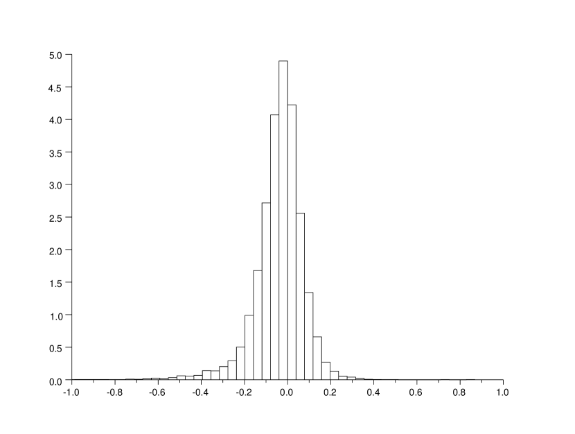
(a) Limit law of $\exp(0.05T)(b-\hat{b}_{T})_{1,1}$.

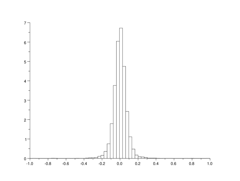
(b) Limit law of $\exp(0.05T)(b-\hat{b}_{T})_{1,2}$.

Figure 1: Asymptotic law of the error for the estimation of $\theta=b$ with for: $x=$ $\left(\begin{smallmatrix}0.5&0.1\\ 0.1&0.3\end{smallmatrix}\right)$, $T=100$, $N=10000$, $\alpha=4.5$ and $b=0.05I_{d}$.

6.2 Experimental convergence in a nonergodic case

In this paragraph, we try to guess the asymptotic behavior of the MLE in a nonergodic case, where no theoretical convergence result is known. Namely, we observe in Figure 2 the asymptotic estimation error, when $b=\operatorname{diag}(0.1,0.005)$ is diagonal with positive and distinct terms on its diagonal and when we use the estimator (27). As one might have guess, the convergence of the diagonal terms seems to be with an exponential rate, with the exponential speed corresponding to its value. Namely, $\hat{b}_{11}$ seems to converge to $b_{11}$ with a speed of $\exp(0.1T)$ while $\hat{b}_{22}$ seems to converge to $b_{22}$ with a speed of $\exp(0.005T)$. More interesting is the antidiagonal term. One could have imagine that the convergence rate is the slowest of these two rates. Instead, on our experiment, the convergence of $\hat{b}_{12}$ towards $b_{12}$ seems to happen with the rate $\exp(0.1T)$. We have observed the same behaviour for other parameter values. Of course, it would be hasty to draw a global conclusion from few particular experiments. However, it is interesting to note that these numerical tests are a way to guess or check the convergence rate of the MLE.

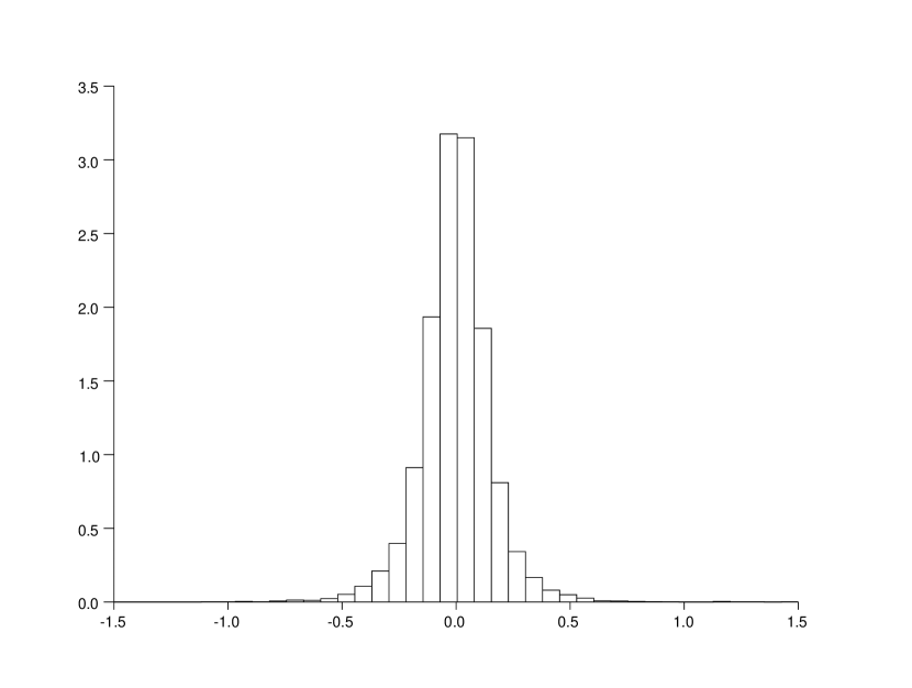
(a) Limit law of $\exp(0.1T)(b-\hat{b}_{T})_{1,1}$.

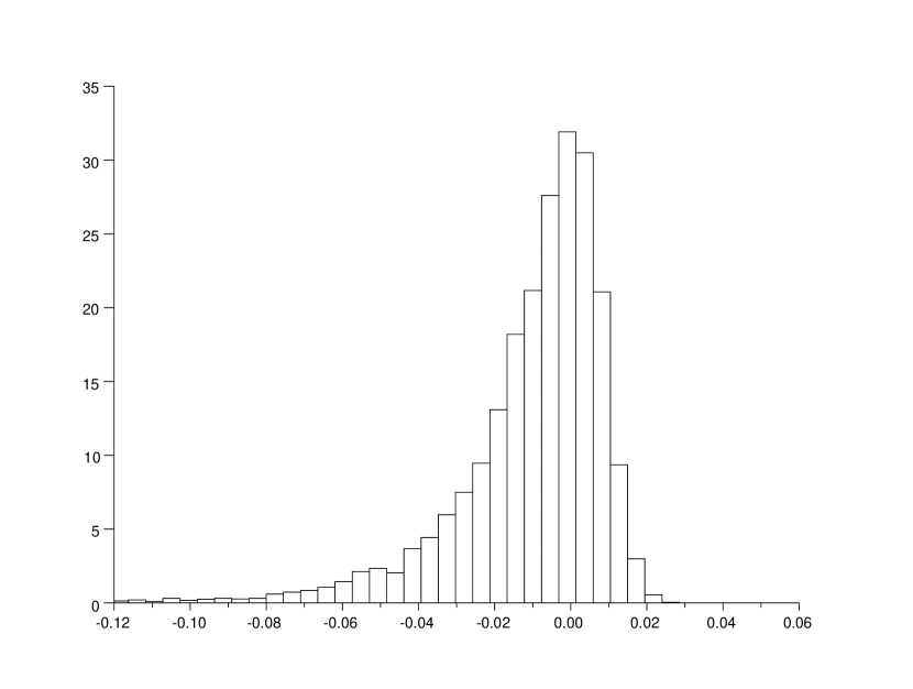
(b) Limit law of $\exp(0.005T)(b-\hat{b}_{T})_{2,2}$.

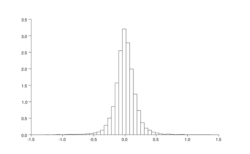
(c) Limit law of $\exp(0.1T)(b-\hat{b}_{T})_{1,2}$.

Figure 2: Asymptotic law of the error for the estimation of $\theta=b$ with $x=$$\left(\begin{smallmatrix}0.3&0.1\\ 0.1&0.2\end{smallmatrix}\right)$, $T=100$, $N=10000$, $\alpha=3.5$ and $b=\operatorname{diag}(0.1,0.005)$.

6.3 Estimation of the whole Wishart process

In this last part of the numerical study, we perform the estimation of all the parameters of the Wishart process (3). We consider a case where $a$ is upper triangular and $(a^{\top})^{-1}ba^{\top}$ is symmetric. We proceed as follows. First, we sample exactly a discrete path $(X_{iT/N},0\leqslant i\leqslant N)$. Then, we estimate the matrix $a^{\top}a$ by using (5), where the quadratic variations are replaced by their classical approximations and the integrals are replaced by the trapezoidal rule. By a Cholesky decomposition we get then an estimator $\hat{a}$ of $a$. Then, we use the MLE (24) on the path $((\hat{a}^{\top})^{-1}X_{iT/N}\hat{a}^{\top},0\leqslant i\leqslant N)$. This gives an estimator of $\alpha$ and $(a^{\top})^{-1}ba^{\top}$, and therefore an estimator of $b$. As a comparison, we also calculate similarly the estimator of $\alpha$ and $b$ when $a$ is known and has not to be estimated. To draw histograms or calculate empirical expectations, we run $M=10000$ independent paths of $X$.

We consider a sufficiently large value of $T$ and are interested in looking at the convergence with respect to $N$. First, we plot the the error on the estimator of $a$ with respect to the number of time step in Log-Log scale. We observe that the convergence to zero takes place with experimental rate close to $1/2$. This is in line with the general results on the estimation of the diffusion coefficient, see Dohnal [12] and Genon-Catalot and Jacod [15]. Then, we focus on the influence of the discretization and the unknown parameter $a$ on the convergence of the MLE of $b$ and $\alpha$. In Table 1, we give in function of $N$ the Mean Squared Error $\operatorname{MSE}(\widehat{\theta}^{N}|\theta)=\mathbb{E}[|\widehat{\theta}^{N}-\theta|^{2}]$ of the estimator $\widehat{\theta}^{N}$, with $\theta=(b,\alpha)$. It is estimated with the empirical expectation. First, we observe that the convergence of the estimator of $\alpha$ is roughly the same whether we know $a$ or not. This is expected since the estimation of $\alpha$ does not depend on the estimation of $a$. Instead, the bias on $b$ is much higher when $a$ is estimated than when $a$ is known. However, it decreases also faster at an experimental order of $0.7$ while the bias when $a$ is known decreases at an experimental order of $0.45$. This latter rate is in line with the rate of $1/2$ obtained in dimension 1 by Ben Alaya and Kebaier [5]. In our case, it seems that the influence of the estimation of $a$ vanishes around $N=5000$. Last, we have plotted in Figure 4 the limit law of the estimator $\sqrt{T}(\widehat{\theta}^{N}-\theta)$ with $N=10000$.

This short numerical study shows that the estimator obtained by discretizing the continuous time estimator is efficient in practice. Of course, it would be nice to obtain general convergence results in function of $T$ and $N$, but we leave this for further research.

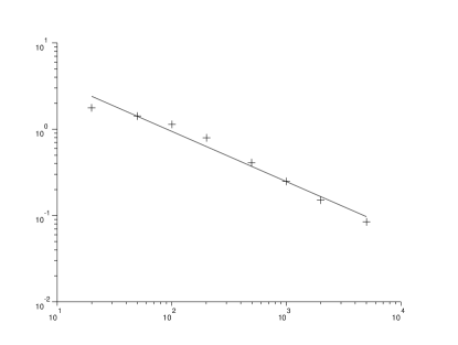
Figure 3: Log-Log representation of the empirical expectation of $\mathbb{E}[\operatorname{Tr}[(a-\widehat{a}^{N})^{2}]]^{1/2}$ for $x=$$\left(\begin{smallmatrix}0.8&0.5\\ 0.5&1\end{smallmatrix}\right)$, $T=100$, $a=$$\left(\begin{smallmatrix}1&1\\ 0&2\end{smallmatrix}\right)$, $\alpha=4.5$, $b=$$\left(\begin{smallmatrix}-1&0.2\\ 2&-2\end{smallmatrix}\right)$, where the line is the simple linear regression i.e. $\log(\mathbb{E}[\operatorname{Tr}[(a-\widehat{a}^{N})^{2}]]^{1/2})\approx 2.62-0.58\log(N)$.

Number of time steps		20	50	100	200	500	1000	2000	5000
$\mathbb{E}[\operatorname{Tr}[(a-\widehat{a}^{N})^{2}]]^{1/2}$		1.7671	1.4311	1.1487	0.7913	0.4107	0.2472	0.1514	0.0846
	$\widehat{a}=a$	0.0745	0.0338	0.0181	0.0115	0.0082	0.0069	0.0061	0.0058
$\operatorname{MSE}(\widehat{b}^{N}_{1,1}|b_{1,1})$	$\widehat{a}=\widehat{a}^{N}$	0.7636	0.5266	0.3489	0.1891	0.0624	0.0273	0.0142	0.0085
	$\widehat{a}=a$	0.2554	0.1310	0.0664	0.0372	0.0231	0.0176	0.0153	0.0139
$\operatorname{MSE}(\widehat{b}^{N}_{2,2}|b_{2,2})$	$\widehat{a}=\widehat{a}^{N}$	3.4085	2.8722	2.1159	1.1995	0.3600	0.1264	0.0480	0.0201
	$\widehat{a}=a$	0.0075	0.0033	0.0017	0.0011	0.0008	0.0008	0.0007	0.0007
$\operatorname{MSE}(\widehat{b}^{N}_{1,2}|b_{1,2})$	$\widehat{a}=\widehat{a}^{N}$	0.0442	0.0568	0.0596	0.0352	0.0148	0.0075	0.0039	0.0019
	$\widehat{a}=a$	0.8448	0.3579	0.1993	0.1151	0.0614	0.0416	0.0308	0.0230
$\operatorname{MSE}(\widehat{\alpha}^{N}|\alpha)$	$\widehat{a}=\widehat{a}^{N}$	0.8267	0.3496	0.1895	0.1095	0.0617	0.0410	0.0311	0.0234

Table 1: Mean Squared Error for the estimation of $\theta=(b,\alpha)$ with respect to $N$. Same parameters as Figure 3.

(a) Limit law of $\sqrt{T}(b-\hat{b}^{N}_{T})_{1,1}$.

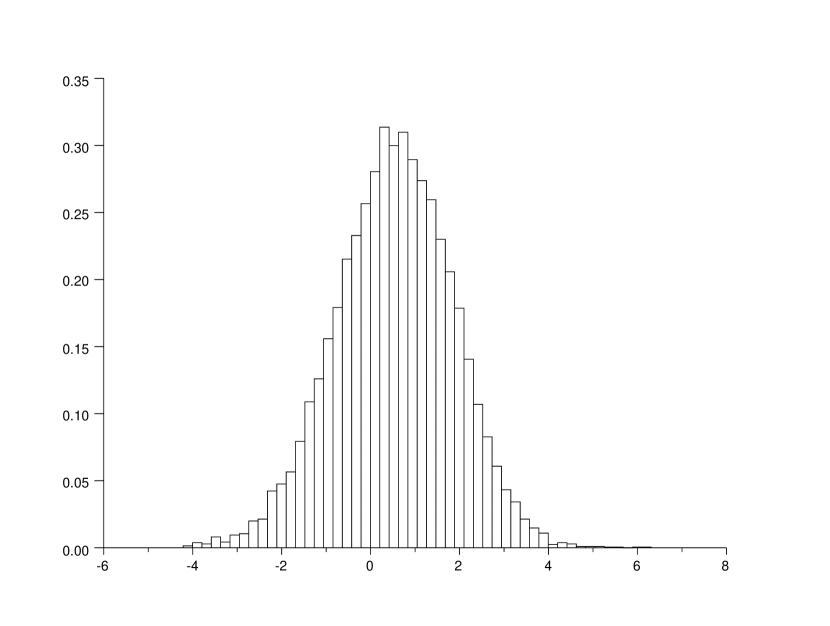
(b) Limit law of $\sqrt{T}(b-\hat{b}^{N}_{T})_{2,2}$.

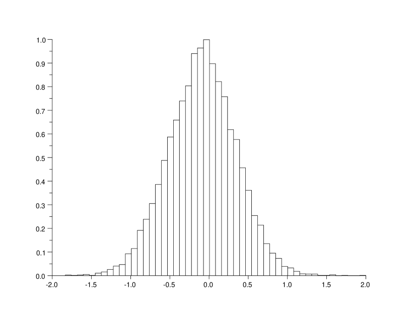
(c) Limit law of $\sqrt{T}(b-\hat{b}^{N}_{T})_{1,2}$.

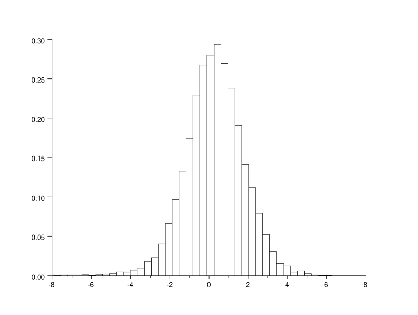
(d) Limit law of $\sqrt{T}(\alpha-\hat{\alpha}^{N}_{T})$.

Figure 4: Asymptotic laws of the error for the estimation of $\theta=(b,\alpha)$ for $\widehat{a}=\widehat{a}^{N}$, $N=10000$, same parameters as Figure 3.

Appendix A Proof of Proposition 1.1

We denote $b^{s}=(b+b^{\top})/2$ (resp. $b^{a}=(b-b^{\top})/2$) the symmetric (resp. antisymmetric) part of $b$. We have

$$\int_{0}^{T}\operatorname{Tr}[(\sqrt{X_{s}})^{-1}dW_{s}] =\frac{1}{2}\log\left(\frac{\det[X_{T}]}{\det[x]}\right)-\operatorname{Tr}[b]T-\frac{1}{2}\int_{0}^{T}(\alpha-1-d)\operatorname{Tr}[X_{s}^{-1}]ds,$$

$$\int_{0}^{T}\operatorname{Tr}[b^{s}\sqrt{X_{s}}dW_{s}] =\frac{1}{2}\int_{0}^{T}\operatorname{Tr}[b^{s}(\sqrt{X_{s}}dW_{s}+dW_{s}^{\top}\sqrt{X_{s}})]$$

$$=\frac{\operatorname{Tr}[b^{s}X_{T}]-{\operatorname{Tr}[b^{s}x]}}{2}-\frac{\alpha T}{2}{\operatorname{Tr}[b^{s}]}-\frac{1}{2}\int_{0}^{T}\operatorname{Tr}[b^{s}(bX_{t}+X_{t}b^{\top})]dt.$$

Thus, the only part to calculate is $\mathbb{E}\left[\exp(\int_{0}^{T}\operatorname{Tr}[-b^{a}\sqrt{X_{s}}dW_{s}])\bigg{|}\mathcal{F}^{X}_{T}\right]$, and we set $M^{a}_{t}=\int_{0}^{t}\operatorname{Tr}[b^{a}\sqrt{X_{s}}dW_{s}]$. We now observe that $\langle\operatorname{Tr}[A_{s}dW_{s}],\operatorname{Tr}[B_{s}dW_{s}]\rangle=\operatorname{Tr}[A_{s}B_{s}^{\top}]ds$ and are looking for the process $\Gamma$ that takes values in ${\mathcal{S}_{d}}$ and minimizes

$$\langle dM^{a}_{t}-\operatorname{Tr}[\Gamma_{t}(dX_{t}-(\alpha I_{d}+bX_{t}+X_{t}b^{\top})dt)]\rangle=\left\{-\operatorname{Tr}[b^{a}X_{t}b^{a}]+2\operatorname{Tr}[\Gamma_{t}(X_{t}b^{a}-b^{a}X_{t})]+4\operatorname{Tr}[\Gamma_{t}^{2}X_{t}]\right\}dt.$$

We obtain that $2(X_{t}b^{a}-b^{a}X_{t})+4(X_{t}\Gamma_{t}+\Gamma_{t}X_{t})=0$ and thus

$$\Gamma_{t}=\mathcal{L}_{X_{t}}^{-1}\left(\frac{1}{2}(b^{a}X_{t}-X_{t}b^{a})\right).$$

It satisfies $\operatorname{Tr}[\Gamma_{t}(X_{t}b^{a}-b^{a}X_{t})]=-2\operatorname{Tr}[\Gamma_{t}(\Gamma_{t}X_{t}+X_{t}\Gamma_{t})]=-4\operatorname{Tr}[\Gamma_{t}^{2}X_{t}]$. By construction, we have $\langle dM^{a}_{t}-\operatorname{Tr}[\Gamma_{t}(dX_{t}-(\alpha I_{d}+bX_{t}+X_{t}b^{\top})dt)],\operatorname{Tr}[\tilde{\Gamma}(dX_{t}-(\alpha I_{d}+bX_{t}+X_{t}b^{\top})dt)]\rangle=0$ for any $\tilde{\Gamma}\in\textbf{${\mathcal{S}_{d}}$}$. Thus, there exists a Brownian motion $\beta$ independent of $X$ such that $dM^{a}_{t}-\operatorname{Tr}[\Gamma_{t}(dX_{t}-(\alpha I_{d}+bX_{t}+X_{t}b^{\top})dt)]=\sqrt{-\operatorname{Tr}[b^{a}X_{t}b^{a}]-\operatorname{Tr}[\Gamma_{t}(b^{a}X_{t}-X_{t}b^{a})]}d\beta_{t}$. In fact, both processes $(X_{t},\int_{0}^{t}\sqrt{-\operatorname{Tr}[b^{a}X_{s}b^{a}]-\operatorname{Tr}[\Gamma_{t}(b^{a}X_{s}-X_{s}b^{a})]}d\beta_{s})$ and

$$(X_{t},M^{a}_{t}-\int_{0}^{t}\operatorname{Tr}[\Gamma_{s}(\sqrt{X_{s}}dW_{s}+dW_{s}^{\top}\sqrt{X_{s}})])$$

solve the same martingale problem for which uniqueness holds. Therefore, we have

$$\mathbb{E}\left[\exp\left(-\int_{0}^{T}\operatorname{Tr}[b^{a}\sqrt{X_{t}}dW_{t}]\right)\bigg{|}\mathcal{F}^{X}_{T}\right]$$

$$= \exp\left(\int_{0}^{T}\operatorname{Tr}\left[\Gamma_{t}((\alpha I_{d}+bX_{t}+X_{t}b^{\top})dt-dX_{t})\right]-\frac{1}{2}\int_{0}^{T}\operatorname{Tr}[b^{a}X_{t}b^{a}]+\operatorname{Tr}[\Gamma_{t}(b^{a}X_{t}-X_{t}b^{a})]dt\right)$$

$$= \exp\left(-\int_{0}^{T}\operatorname{Tr}\left[\mathcal{L}_{X_{t}}^{-1}\left(\frac{1}{2}(b^{a}X_{t}-X_{t}b^{a})\right)dX_{t}\right]-\int_{0}^{T}\frac{1}{2}\operatorname{Tr}[b^{a}X_{t}b^{a}]dt\right.$$

$$\left.+\frac{1}{2}\int_{0}^{T}\operatorname{Tr}\left[\mathcal{L}_{X_{t}}^{-1}\left(\frac{1}{2}(b^{a}X_{t}-X_{t}b^{a})\right)(b^{a}X_{t}-X_{t}b^{a})\right]dt+\int_{0}^{T}\operatorname{Tr}[b^{a}X_{t}b^{s}]dt\right),$$

since $\operatorname{Tr}\left[\mathcal{L}_{X_{t}}^{-1}\left(\frac{1}{2}(b^{a}X_{t}-X_{t}b^{a})\right)\right]=\frac{1}{2}\operatorname{Tr}[X_{t}^{-1}(b^{a}X_{t}-X_{t}b^{a})]=0$ by Lemma B.1 and

$$\operatorname{Tr}[\Gamma_{t}(b^{s}X_{t}+X_{t}b^{s})]=\operatorname{Tr}[b^{s}(\Gamma_{t}X_{t}+X_{t}\Gamma_{t})]=\frac{1}{2}\operatorname{Tr}\left[b^{s}(b^{a}X_{t}-X_{t}b^{a})\right]=\operatorname{Tr}[b^{a}X_{t}b^{s}].$$

Using (8) and the previous calculations, we obtain

$$L_{T}^{\theta,\theta_{0}}=\exp\Bigl{(}\frac{\alpha-\alpha_{0}}{4}\log\left(\frac{\det[X_{T}]}{\det[x]}\right)+\frac{\operatorname{Tr}[b^{s}X_{T}]-{\operatorname{Tr}[b^{s}x]}}{2}-\frac{1}{2}\int_{0}^{T}\operatorname{Tr}[(b^{s})^{2}X_{s}]ds\\ -\int_{0}^{T}\operatorname{Tr}[b^{a}X_{s}b^{s}]ds-\frac{\alpha-\alpha_{0}}{4}\big{(}\frac{\alpha+\alpha_{0}}{2}-1-d\big{)}\int_{0}^{T}\operatorname{Tr}[X_{s}^{-1}]ds-\frac{\alpha T}{2}\operatorname{Tr}[b]\\ +\frac{1}{2}\int_{0}^{T}\operatorname{Tr}\left[\mathcal{L}_{X_{t}}^{-1}\left(b^{a}X_{t}-X_{t}b^{a}\right)dX_{t}\right]-\frac{1}{4}\int_{0}^{T}\operatorname{Tr}\left[\mathcal{L}_{X_{t}}^{-1}\left(b^{a}X_{t}-X_{t}b^{a}\right)(b^{a}X_{t}-X_{t}b^{a})\right]dt\Bigr{)}.$$

Last, we use $\mathcal{L}_{X_{t}}^{-1}\left(b^{s}X_{t}+X_{t}b^{s}\right)=b^{s}$ and $\operatorname{Tr}[\mathcal{L}_{X_{t}}^{-1}\left(b^{a}X_{t}-X_{t}b^{a}\right)(b^{s}X_{t}+X_{t}b^{s})]=2\operatorname{Tr}[b^{a}X_{t}b^{s}]$ to obtain (9).

Appendix B Technical lemmas

Lemma B.1.

For $X\in\textbf{${\mathcal{S}_{d}^{+,*}}$}$ and $a\geqslant 0$, let ${\mathcal{L}}_{X,a}$ and $\mathcal{L}_{X}={\mathcal{L}}_{X,0}$ be the linear applications defined by (18) on $\mathcal{S}_{d}$. If $a\operatorname{Tr}[X^{-1}]\neq 1$, then ${\mathcal{L}}_{X,a}$ is invertible and we have $\operatorname{Tr}[\mathcal{L}^{-1}_{X,a}(Y)]=\frac{\operatorname{Tr}[X^{-1}Y]}{2(1-a\operatorname{Tr}[X^{-1}])}$. Besides, the map $(X,Y,a)\mapsto\mathcal{L}^{-1}_{X,a}(Y)$ is continuous on $\{(X,Y,a)\in\textbf{${\mathcal{S}_{d}^{+,*}}$}\times\textbf{${\mathcal{S}_{d}}$}\times\mathbb{R}_{+},\ a\operatorname{Tr}[X^{-1}]\neq 1\}$.

Proof.

The invertibility of ${\mathcal{L}}_{X,a}$ is equivalent to its one-to-one property. Since $X\in\mathcal{S}_{d}^{+,*}$, there exists an orthogonal matrix $O_{X}$ and a diagonal matrix $D_{X}$ with positive elements such that $X=O_{X}D_{X}O_{X}^{\top}$. We get

$$Y\in\ker({\mathcal{L}}_{X,a})\iff O_{X}D_{X}O_{X}^{\top}Y+YO_{X}D_{X}O_{X}^{\top}=2a\operatorname{Tr}[Y]I_{d}$$

$$\iff D_{X}(O^{\top}_{X}YO_{X})=2a\operatorname{Tr}[Y]I_{d}-(O_{X}^{\top}YO_{X})D_{X}.$$ (81)

Since $D_{X}$ is diagonal, we obtain for $1\leqslant i,k\leqslant d$, $\left((O^{\top}_{X}YO_{X})D_{X}\right)_{i,k}=(O^{\top}_{X}YO_{X})_{i,k}(D_{X})_{k,k}$ and $\left(D_{X}(O^{\top}_{X}YO_{X})\right)_{i,k}=(D_{X})_{i,i}(O^{\top}_{X}YO_{X})_{i,k}$. For $k\not=i$, (81) gives $(O^{\top}_{X}YO_{X})_{i,k}=0$. For $k=i$, we get $(O^{\top}_{X}YO_{X})_{i,i}(D_{X})_{i,i}=a\operatorname{Tr}[Y]$ and therefore

$$\operatorname{Tr}[Y]=\operatorname{Tr}[O^{\top}_{X}YO_{X}]=\operatorname{Tr}[Y]a\sum_{i=1}^{d}\frac{1}{(D_{X})_{i,i}}=\operatorname{Tr}[Y]a\operatorname{Tr}[X^{-1}].$$

Since $a\operatorname{Tr}[X^{-1}]\not=1$, we obtain $\operatorname{Tr}[Y]=0$ and then $(O^{\top}_{X}YO_{X})_{i,i}=0$, which gives $Y=0$ and the invertibility of ${\mathcal{L}}_{X,a}$. Let $c=\mathcal{L}_{X,a}^{-1}(Y)$. We have $c+X^{-1}cX-2a\operatorname{Tr}[c]X^{-1}=X^{-1}Y$, which gives $2(1-a\operatorname{Tr}[X^{-1}])\operatorname{Tr}[c]=\operatorname{Tr}[X^{-1}Y].$ Last, the continuity property is obvious since $(X,a)\mapsto\mathcal{L}_{X,a}$ is continuous and $\mathcal{L}\mapsto\mathcal{L}^{-1}$ is continuous on $\{\mathcal{L}:\textbf{${\mathcal{S}_{d}}$}\rightarrow\textbf{${\mathcal{S}_{d}}$}\text{ linear and invertible}\}$. ∎

Lemma B.2.

For $X\in\textbf{${\mathcal{S}_{d}^{+,*}}$}$, $\mathcal{L}_{X}$ is self-adjoint and positive definite:

$$\operatorname{Tr}[\mathcal{L}_{X}(Y)Y]\geq 2\underline{\lambda}(X)\operatorname{Tr}[Y^{2}],$$

where $\underline{\lambda}(X)>0$ is the lowest eigenvalue of $X$. Besides, for $a<1/\operatorname{Tr}[X^{-1}]$, $\mathcal{L}_{X,a}$ is self-adjoint and positive definite.

Proof.

For $Y,Z\in\textbf{${\mathcal{S}_{d}}$}$, we have $\operatorname{Tr}[\mathcal{L}_{X}(Y)Z]=\operatorname{Tr}[(XY+YX)Z]=\operatorname{Tr}[Y(XZ+ZX)]=\operatorname{Tr}[Y\mathcal{L}_{X}(Z)]$ and $\operatorname{Tr}[\mathcal{L}_{X}(Y)Y]=2\operatorname{Tr}[XY^{2}]\geq 2\underline{\lambda}(X)\operatorname{Tr}[Y^{2}]$ since $X-\underline{\lambda}(X)I_{d}\in\textbf{${\mathcal{S}_{d}^{+}}$}$. The self-adjoint property is then clear for $\mathcal{L}_{X,a}$, and the positive definiteness comes from Lemma B.1 and the continuity of the eigenvalues of $\mathcal{L}_{X,a}$ with respect to $a$. ∎

Lemma B.3.

For $X\in\textbf{${\mathcal{S}_{d}^{+,*}}$}$, $Y\in\textbf{${\mathcal{M}_{d}}$}$, $\bar{\mathcal{L}}_{X}(Y)=\mathcal{L}_{X}^{-1}(YX+XY^{\top})X$ is self-adjoint and positive. The linear application $\bar{\mathcal{L}}_{X,a}(Y)=\mathcal{L}_{X}^{-1}(YX+XY^{\top})X-a\operatorname{Tr}[Y]I_{d}$ is also positive for $a<1/\operatorname{Tr}[X^{-1}]$, and there is a positive $c_{X,a}>0$ such that

$$\operatorname{Tr}[\bar{\mathcal{L}}_{X}(Y)^{\top}Y]\geq c_{X,a}\operatorname{Tr}[(\mathcal{L}_{X}^{-1}(YX+XY^{\top}))^{2}].$$

Proof.

Since $\mathcal{L}_{X}^{-1}$ is self-adjoint, we have for $Z\in\textbf{${\mathcal{M}_{d}}$}$

$$\operatorname{Tr}[\bar{\mathcal{L}}_{X}(Y)^{\top}Z] =\operatorname{Tr}[\mathcal{L}_{X}^{-1}(YX+XY^{\top})ZX]=\frac{1}{2}\operatorname{Tr}[\mathcal{L}_{X}^{-1}(YX+XY^{\top})(ZX+XZ^{\top})]$$

$$=\frac{1}{2}\operatorname{Tr}[(YX+XY^{\top})\mathcal{L}_{X}^{-1}(ZX+XZ^{\top})]=\operatorname{Tr}[Y^{\top}\bar{\mathcal{L}}_{X}(Z)].$$

Similarly, $\operatorname{Tr}[\bar{\mathcal{L}}_{X,a}(Y)^{\top}Z]=\operatorname{Tr}[\bar{\mathcal{L}}_{X}(Y)^{\top}Z]-a\operatorname{Tr}[Y]\operatorname{Tr}[Z]=\operatorname{Tr}[Y^{\top}\bar{\mathcal{L}}_{X,a}(Z)]$. Besides, we notice that

$$\operatorname{Tr}[\bar{\mathcal{L}}_{X,a}(Y)^{\top}Y] =\frac{1}{2}\left(\operatorname{Tr}[(YX+XY^{\top})\mathcal{L}_{X}^{-1}(YX+XY^{\top})]-2a\operatorname{Tr}[Y]^{2}\right)$$

$$=\frac{1}{2}\left(\operatorname{Tr}[\mathcal{L}_{X,a}(\mathcal{L}_{X}^{-1}(YX+XY^{\top}))\mathcal{L}_{X}^{-1}(YX+XY^{\top})]\right)$$

by Lemma B.1. This gives the claim since $\mathcal{L}_{X,a}$ is positive definite by Lemma B.2. ∎

The following lemma gives the Laplace transform of the matrix Normal distribution.

Lemma B.4.

Let $C\in\mathcal{S}_{d}^{+,*}$ and $\mathscr{C}[C]\in(\mathbb{R}^{d})^{\otimes 4}$ defined by

$$\mathscr{C}[C]_{i,j,k,l}=\delta_{ik}C_{j,l}+\delta_{il}C_{j,k}+\delta_{jk}C_{i,l}+\delta_{jl}C_{i,k}.$$ (82)

We introduce the $\mathcal{M}_{d}$-valued random variables $\tilde{\mathbf{G}}$ and $\mathbf{G}\sim\mathcal{N}(0,\mathscr{C}[C])$ of which components are Normal random variables with mean $0$ such that

$$\forall i,j,k,l\in\{1,\dots,d\},\quad\mathbb{E}[\tilde{\mathbf{G}}_{i,j}\tilde{\mathbf{G}}_{k,l}]=\delta_{ik}\delta_{jl},\quad\mathbb{E}[\mathbf{G}_{i,j}\mathbf{G}_{k,l}]=\mathscr{C}[C]_{i,j,k,l}.$$ (83)

We have the following results.

1. For all $c\in\mathcal{S}_{d}$, $\mathbb{E}\big{[}\exp(-\operatorname{Tr}[c\mathbf{G}])\big{]}=\exp(2\operatorname{Tr}[c^{2}C])$.

2. For $\tilde{C}\in\textbf{${\mathcal{M}_{d}}$}$ such that $\tilde{C}\tilde{C}^{\top}=C$, $\tilde{C}\tilde{\mathbf{G}}+\tilde{\mathbf{G}}^{\top}\tilde{C}^{\top}$ and $\mathbf{G}$ have the same law.

3. Let $X\in\textbf{${\mathcal{S}_{d}^{+,*}}$}$. For $c\in\textbf{${\mathcal{S}_{d}}$}$, $\mathbb{E}[\exp(-\operatorname{Tr}[c\mathcal{L}_{X}^{-1}(\sqrt{X}\tilde{\mathbf{G}}+\tilde{\mathbf{G}}^{\top}\sqrt{X})])]=\mathbb{E}[\exp(\operatorname{Tr}[c\mathcal{L}_{X}^{-1}(c)])$

Proof.

We focus on the first point. For all $c\in\mathcal{S}_{d}$, we have

$$\mathbb{E}\big{[}\exp(-\operatorname{Tr}[c\mathbf{G}])\big{]}=\mathbb{E}\big{[}\exp(-\sum_{1\leqslant i,j\leqslant d}c_{i,j}\mathbf{G}_{i,j})\big{]}.$$

Moreover, $\sum_{1\leqslant i,j\leqslant d}c_{i,j}\mathbf{G}_{i,j}$ is a Normal random variable and its variance is given by

$$\mathbb{E}\big{[}\big{(}\sum_{1\leqslant i,j\leqslant d}c_{i,j}\mathbf{G}_{i,j}\big{)}^{2}\big{]}= \sum_{1\leqslant i,j,k,l\leqslant d}c_{i,j}c_{k,l}\mathscr{C}[C]_{i,j,k,l}=4\operatorname{Tr}[c^{2}C].$$

It follows from the moment generating function of the Normal distribution that

$$\mathbb{E}\big{[}\exp(-\operatorname{Tr}[c\mathbf{G}])\big{]}=\exp(2\operatorname{Tr}[c^{2}C]).$$

To prove the second point it is sufficient to notice that $\operatorname{Tr}[c(\tilde{C}\tilde{\mathbf{G}}+\tilde{\mathbf{G}}^{\top}\tilde{C}^{\top})]=\operatorname{Tr}[2c\tilde{C}\tilde{\mathbf{G}}]$ and

$$\mathbb{E}\big{[}\big{(}\sum_{1\leqslant i,j\leqslant d}(c\tilde{C})_{i,j}\tilde{\mathbf{G}}_{i,j}\big{)}^{2}\big{]}= \sum_{1\leqslant i,j,k,l\leqslant d}(c\tilde{C})_{i,j}(c\tilde{C})_{k,l}\delta_{ik}\delta_{jl}=\sum_{1\leqslant i,j\leqslant d}(c\tilde{C})_{i,j}^{2}=\operatorname{Tr}[c\tilde{C}\tilde{C}^{\top}c].$$

For the third point, we set $Z=\mathcal{L}_{X}^{-1}(\sqrt{X}\tilde{\mathbf{G}}+\tilde{\mathbf{G}}^{\top}\sqrt{X})$ and have $XZ+ZX=\sqrt{X}\tilde{\mathbf{G}}+\tilde{\mathbf{G}}^{\top}\sqrt{X}$. We also introduce $\tilde{c}=\mathcal{L}_{X}^{-1}(c)$ and have $\tilde{c}X+X\tilde{c}=c$. Thus, we obtain

$$\operatorname{Tr}[cZ] =\operatorname{Tr}[(\tilde{c}X+X\tilde{c})Z]=\operatorname{Tr}[\tilde{c}(\sqrt{X}\tilde{\mathbf{G}}+\tilde{\mathbf{G}}^{\top}\sqrt{X})]$$

and therefore $\mathbb{E}[\exp(-\operatorname{Tr}[cZ])]=\exp(2\operatorname{Tr}[\tilde{c}^{2}X])=\exp(\operatorname{Tr}[\tilde{c}(\tilde{c}X+X\tilde{c})])=\exp(\operatorname{Tr}[\tilde{c}c])$.

∎

Appendix C Some asymptotic behaviour of Wishart processes

Lemma C.1.

Let $X\sim WIS_{d}(x,\alpha,b,I_{d})$ with $b\in\textbf{${\mathcal{S}_{d}}$}$, $x\in\textbf{${\mathcal{S}_{d}^{+}}$}$ and $\alpha\geqslant d-1$. Then $X_{T}$ converges in law when $T\rightarrow+\infty$ if and only if $-b\in\textbf{${\mathcal{S}_{d}^{+,*}}$}$. In this case, $X_{T}$ converges in law to $WIS_{d}(0,\alpha,0,\sqrt{-b^{-1}};1/2)$.

Let $X\sim WIS_{d}(x,\alpha,b,I_{d})$ with $b\in\textbf{${\mathcal{M}_{d}}$}$, $x\in\textbf{${\mathcal{S}_{d}^{+}}$}$ and $\alpha\geqslant d-1$. If $-(b+b^{\top})\in\textbf{${\mathcal{S}_{d}^{+,*}}$}$, $q_{\infty}:=\int_{0}^{\infty}e^{sb}e^{sb^{\top}}ds$ is well defined and $X_{T}$ converges in law to $WIS_{d}(0,\alpha,0,\sqrt{2q_{\infty}};1/2)$.

Proof.

Let us first consider the case $-b\in\textbf{${\mathcal{S}_{d}^{+,*}}$}$. From Proposition 4 in [2], we have for $v\in\textbf{${\mathcal{S}_{d}^{+}}$}$,

$$\mathbb{E}[\exp(-\operatorname{Tr}[vX_{T}])] =\frac{\exp\left(\operatorname{Tr}\left[-v\left(I_{d}+2\left(\int_{0}^{T}e^{2bs}ds\right)v\right)^{-1}e^{Tb}xe^{Tb}\right]\right)}{\det\left[I_{d}+2\left(\int_{0}^{T}e^{2bs}ds\right)v\right]^{\alpha/2}}$$

$$\underset{T\rightarrow+\infty}{\rightarrow}\frac{1}{\det\left[I_{d}-b^{-1}v\right]^{\alpha/2}},$$

which is the Laplace transform of $WIS_{d}(0,\alpha,0,\sqrt{-b^{-1}};1/2)$. Now, let us consider $-b\not\in\textbf{${\mathcal{S}_{d}^{+,*}}$}$. Then, there exists an eigenvector $v\in\mathbb{R}^{d}\setminus\{0\}$ such that $bv=\lambda v$ with $\lambda\geqslant 0$. Then, we have $\frac{d}{dt}\mathbb{E}[v^{\top}X_{t}v]=\alpha v^{\top}v+2\lambda\mathbb{E}[v^{\top}X_{t}v]$, and therefore $\mathbb{E}[v^{\top}X_{T}v]\underset{T\rightarrow+\infty}{\rightarrow}+\infty$.

In the case $b\in\textbf{${\mathcal{M}_{d}}$}$ with $-(b+b^{\top})\in\textbf{${\mathcal{S}_{d}^{+,*}}$}$, we know that the norm of $e^{bs}$ decays exponentially to $0$ as $s\rightarrow+\infty$, see e.g. Problem 11.3.6 in Golub and Van Loan [18]. Using again Proposition 4 in [2], we get that $\mathbb{E}[\exp(-\operatorname{Tr}[vX_{T}])]\underset{T\rightarrow+\infty}{\rightarrow}\frac{1}{\det\left[I_{d}+2q_{\infty}v\right]^{\alpha/2}}$. ∎

Lemma C.2.

$\bullet$ Assume $\alpha>d+1$ and $b=0$. Then, $\frac{Q_{T}^{-1}}{d\log(T)}\underset{T\rightarrow+\infty}{\rightarrow}\frac{1}{\alpha-(d+1)}$ a.s. Besides, $\frac{Z_{T}}{\log(T)}$ converges almost surely to $d$, and we have

$$\forall\mu>0,\sup_{T\geqslant 2}\mathbb{E}\left[\exp\left(\frac{\mu}{\sqrt{\log(T)}}N_{T}\right)\right]<\infty.$$ (84)

$\bullet$ Assume $\alpha=d+1$ and $b=0$. Then, as $T\rightarrow+\infty$, $\left(\frac{2}{d\log(T)}\right)^{2}Q_{T}^{-1}$ converges in law to $\tau_{1}=\inf\{t\geqslant 0,B_{t}=1\}$, where $B$ is a Brownian motion. Besides, $\frac{Z_{T}}{\log(T)}=\frac{2N_{T}}{\log(T)}$ converges in probability to $d$, and we have

$$\forall\mu>0,\sup_{T\geqslant 2}\mathbb{E}\left[\exp\left(\frac{\mu}{{\log(T)}}N_{T}\right)\right]<\infty.$$ (85)

We mention that the results on the convergence for $Q_{T}$ are given in Donati-Martin et al. [13]. However, their proofs is in a working paper by the same authors that we have not been able to find. For this reason, we present here an autonomous proof.

Proof.

We first consider the case $\alpha>d+1$. We have $dX_{t}=\alpha I_{d}dt+\sqrt{X_{t}}dW_{t}+dW_{t}^{\top}\sqrt{X_{t}}$ and thus

$$d(e^{-t}X_{e^{t}-1})=[\alpha I_{d}-e^{-t}X_{e^{t}-1}]dt+\sqrt{e^{-t}X_{e^{t}-1}}d\tilde{W}_{t}+d\tilde{W}_{t}^{\top}\sqrt{e^{-t}X_{e^{t}-1}},$$

with $d\tilde{W}_{t}=e^{-t/2}d(W_{e^{t}-1})$. We observe that $\tilde{W}$ is a matrix Brownian motion, which gives $Y\sim WIS_{d}(x,\alpha,-I_{d}/2,I_{d})$, where $Y_{t}=e^{-t}X_{e^{t}-1}$ for $t\geqslant 0$. Using equation (34) to the process $Y$, we get

$$\frac{1}{t}\log\left(\frac{\det[Y_{t}]}{\det[Y_{0}]}\right)=(\alpha-1-d)\frac{1}{t}\int_{0}^{t}\operatorname{Tr}[Y^{-1}_{s}]ds-d+\frac{2}{t}\int_{0}^{t}\operatorname{Tr}[\sqrt{Y^{-1}_{s}}d\tilde{W}_{s}].$$ (86)

Since $Y$ is ergodic and $\langle\int_{0}^{t}\operatorname{Tr}[\sqrt{Y^{-1}_{s}}d\tilde{W}_{s}]\rangle=\int_{0}^{t}\operatorname{Tr}[Y^{-1}_{s}]ds$, we get that the left hand side converges in probability to zero and the right hand side converges a.s. to $(\alpha-1-d)\mathbb{E}[\operatorname{Tr}[Y^{-1}_{\infty}]]-d$, where $Y_{\infty}\sim WIS_{d}(0,\alpha,0,\sqrt{2}I_{d};1/2)$ is the stationary law of $Y$. Therefore, $\frac{1}{t}\log\left(\frac{\det[Y_{t}]}{\det[Y_{0}]}\right)$ converges a.s. to zero. Since $\frac{1}{t}\log\left(\frac{\det[Y_{t}]}{\det[Y_{0}]}\right)=\frac{1}{t}\log\left(\frac{\det[e^{-t}X_{e^{t}-1}]}{\det[x]}\right)=\frac{1}{t}\log\left(\frac{\det[X_{e^{t}-1}]}{\det[x]}\right)-d$, we get that $\frac{Z_{T}}{\log(T)}=\frac{1}{\log(T)}\log\left(\frac{\det[X_{T}]}{\det[x]}\right)$ converges a.s. to $d$ when $T\rightarrow+\infty$.

Now, we use (34) taken at time $T=e^{t}-1$ and Dubins-Schwarz theorem: there is a Brownian motion $\beta$ such that for all $t\geqslant 0$,

$$\frac{\alpha-(1+d)}{Q_{e^{t}-1}t}+\frac{2\beta_{Q^{-1}_{e^{t}-1}}}{t}=\frac{1}{t}\log\left(\frac{\det[X_{e^{t}-1}]}{\det[x]}\right).$$

This gives that $\frac{\alpha-(1+d)}{Q_{e^{t}-1}t}\underset{t\rightarrow+\infty}{\rightarrow}d$ a.s., and therefore $\frac{Q_{T}^{-1}}{d\log(T)}\underset{T\rightarrow+\infty}{\rightarrow}\frac{1}{\alpha-(d+1)}$, a.s.

It remains to prove (84). From (34), we have $N_{T}=\frac{Z_{T}}{2}-\frac{\alpha-1-d}{2}Q_{T}^{-1}\leq\frac{Z_{T}}{2}$ and thus $\mathbb{E}\left[\exp\left(\frac{\mu}{\sqrt{\log(T)}}N_{T}\right)\right]\leqslant\mathbb{E}\left[\left(\frac{\det[X_{T}]}{\det[x]}\right)^{\frac{\mu}{2\sqrt{\log(T)}}}\right]<\infty$, since the moments of $X$ are bounded. Again we set $t=\log(T+1)$, and for $\Lambda\in[0,1]$, we have from (86)

$$N_{T} =\int_{0}^{T}\operatorname{Tr}[\sqrt{X^{-1}_{s}}dW_{s}]=\int_{0}^{t}\operatorname{Tr}[\sqrt{Y^{-1}_{s}}d\tilde{W}_{s}]$$

$$=\Lambda\int_{0}^{t}\operatorname{Tr}[\sqrt{Y^{-1}_{s}}d\tilde{W}_{s}]+(1-\Lambda)\left(\frac{1}{2}\log\left(\frac{\det[Y_{t}]}{\det[x]}\right)+\frac{d}{2}t-\frac{\alpha-1-d}{2}\int_{0}^{t}\operatorname{Tr}[Y_{s}^{-1}]ds\right).$$

By Cauchy-Schwarz inequality, we get

$$\mathbb{E}\left[\exp\left(\frac{\mu}{\sqrt{\log(T+1)}}N_{T}\right)\right]$$

$$\leq e^{\frac{\mu d(1-\Lambda)}{2}\sqrt{t}}\mathbb{E}^{\frac{1}{2}}\left[\left(\frac{\det[Y_{t}]}{\det[x]}\right)^{(1-\Lambda)\frac{\mu}{\sqrt{t}}}\right]$$

$$\times\mathbb{E}^{\frac{1}{2}}\left[\exp\left(\frac{2\mu\Lambda}{\sqrt{t}}\int_{0}^{t}\operatorname{Tr}[\sqrt{Y^{-1}_{s}}d\tilde{W}_{s}]-\mu(1-\Lambda)\frac{\alpha-1-d}{\sqrt{t}}\int_{0}^{t}\operatorname{Tr}[Y_{s}^{-1}]ds\right)\right].$$

We now take $\Lambda=\Lambda_{t}=\frac{1}{2\epsilon_{t}}\left(-1+\sqrt{1+4\epsilon_{t}}\right)$ with $\epsilon_{t}=\frac{2\mu}{(\alpha-1-d)\sqrt{t}}$ in order to obtain$\frac{1}{2}\left(\frac{2\mu\Lambda_{t}}{\sqrt{t}}\right)^{2}=\mu(1-\Lambda_{t})\frac{\alpha-1-d}{\sqrt{t}}.$ We note that for $t$ large enough, $\Lambda_{t}\in[0,1]$. Besides, we have $\Lambda_{t}\underset{t\rightarrow+\infty}{=}1-\epsilon_{t}+o(1/t)$, so that $\sqrt{t}(1-\Lambda_{t})$ converges to $\frac{2\mu}{\alpha-1-d}$. From Theorem 4.1 in [29], the second expectation is then equal to $1$, while the first one is bounded since $Y$ is ergodic. This yields to (84).

We now consider the case $\alpha=d+1$. We set again $t=\log(1+T)$ and have $T=e^{t}-1$. Thus,

$$Z_{T}=\log\left(\frac{\det[X_{T}]}{\det[x]}\right)=\log\left(\frac{\det[e^{t}Y_{t}]}{\det[x]}\right)=\log\left(\frac{\det[Y_{t}]}{\det[x]}\right)+dt.$$

Again, $Y_{t}$ converges in law towards $WIS_{d}(0,\alpha,0,\sqrt{2}I_{d};1/2)$. Therefore, the ergodic theorem gives that $\frac{1}{t}\log\left(\frac{\det[Y_{t}]}{\det[x]}\right)$ converges in probability to $0$, which yields to the convergence in probability of $\frac{Z_{T}}{\log(T)}$ to $d$. We now turn to the convergence of $\left(\frac{2}{d\log(T)}\right)^{2}Q_{T}^{-1}$. We know from Theorem 4.1 in Mayerhofer [29] that for $T>0$ and $\lambda\geqslant 0$,

$$\mathbb{E}\left[\exp\left(\frac{2\lambda}{d\log(1+T)}N_{T}-\frac{(2\lambda)^{2}}{2d^{2}\log(1+T)^{2}}Q_{T}^{-1}\right)\right]=1.$$

From (34), we have $N_{T}=Z_{T}/2$ and we write

$$1= \mathbb{E}\left[\exp\left(\lambda-\frac{(2\lambda)^{2}}{2d^{2}\log(1+T)^{2}}Q_{T}^{-1}\right)\right]$$

$$+\mathbb{E}\left[\exp\left(-\frac{(2\lambda)^{2}}{2d^{2}\log(1+T)^{2}}Q_{T}^{-1}\right)\left(\exp\left(\frac{2\lambda}{d\log(1+T)}N_{T}\right)-\exp(\lambda)\right)\right]$$

We now observe that $\exp\left(-\frac{(2\lambda)^{2}}{2d^{2}\log(1+T)^{2}}Q_{T}^{-1}\right)\leqslant 1$ and that

$$\mathbb{E}\left[\exp\left(\frac{2\lambda}{d\log(1+T)}N_{T}\right)\right]=\mathbb{E}\left[\left(\frac{\det[X_{T}]}{\det[x]}\right)^{\frac{\lambda}{d\log(1+T)}}\right]=e^{\lambda}\mathbb{E}\left[\left(\frac{\det[Y_{t}]}{\det[x]}\right)^{\frac{\lambda}{dt}}\right].$$

Since $Y$ has bounded moments and is stationary, $\sup_{t\geqslant 1}\mathbb{E}\left[\left(\frac{\det[Y_{t}]}{\det[x]}\right)^{\frac{\lambda}{dt}}\right]<\infty$. This gives the uniform integrability (85) and that

$$\mathbb{E}\left[\exp\left(-\frac{(2\lambda)^{2}}{2d^{2}\log(1+T)^{2}}Q_{T}^{-1}\right)\left(\exp\left(\frac{2\lambda}{d\log(1+T)}N_{T}\right)-\exp(\lambda)\right)\right]\underset{T\rightarrow+\infty}{\rightarrow}0.$$

Therefore, $\lim_{T\rightarrow+\infty}\mathbb{E}\left[\exp\left(\lambda-\frac{(2\lambda)^{2}}{2d^{2}\log(1+T)^{2}}Q_{T}^{-1}\right)\right]=1$, which gives the desired convergence in law. ∎

Acknowledgements. The authors would like to thank Arnaud Gloter (University of Evry) and Marina Kleptsyna (University of Le Mans) for helpful discussions, and the two anonymous referees for their fruitful comments.

References

• [1] A. Ahdida and A. Alfonsi. Exact and high-order discretization schemes for Wishart processes and their affine extensions. Ann. Appl. Probab., 23(3):1025–1073, 2013.
• [2] A. Ahdida, A. Alfonsi, and E. Palidda. Smile with the Gaussian term structure model. Working paper, 2014.
• [3] A. Alfonsi. Affine diffusions and related processes: simulation, theory and applications, volume 6 of Bocconi & Springer Series. Springer, Cham; Bocconi University Press, Milan, 2015.
• [4] M. Ben Alaya and A. Kebaier. Parameter estimation for the square-root diffusions: ergodic and nonergodic cases. Stoch. Models, 28(4):609–634, 2012.
• [5] M. Ben Alaya and A. Kebaier. Asymptotic behavior of the maximum likelihood estimator for ergodic and nonergodic square-root diffusions. Stoch. Anal. Appl., 31(4):552–573, 2013.
• [6] M. Bru. Thèse $3^{\text{\`{e}me}}$ cycle. Résistance d’Escherichia coli aux antibiotiques: Sensibilités des analyses en composantes principales aux perturbations Browniennes et simulation. PhD thesis, Université Paris Nord, 1987.
• [7] M. Bru. Wishart processes. J. Theoret. Probab., 4(4):725–751, 1991.
• [8] C. Cuchiero, D. Filipović, E. Mayerhofer, and J. Teichmann. Affine processes on positive semidefinite matrices. Ann. Appl. Probab., 21(2):397–463, 2011.
• [9] J. Da Fonseca, M. Grasselli, and F. Ielpo. Estimating the Wishart affine stochastic correlation model using the empirical characteristic function. Stud. Nonlinear Dyn. Econom., 18(3):253–289, 2014.
• [10] J. Da Fonseca, M. Grasselli, and C. Tebaldi. Option pricing when correlations are stochastic: an analytical framework. Review of Derivatives Research, 10:151–180, 2008.
• [11] L. Dieci and T. Eirola. Positive definiteness in the numerical solution of Riccati differential equations. Numer. Math., 67(3):303–313, 1994.
• [12] G. Dohnal. On estimating the diffusion coefficient. J. Appl. Probab., 24(1):105–114, 1987.
• [13] C. Donati-Martin, Y. Doumerc, H. Matsumoto, and M. Yor. Some properties of the Wishart processes and a matrix extension of the Hartman-Watson laws. Publ. Res. Inst. Math. Sci., 40(4):1385–1412, 2004.
• [14] E. Fournié and D. Talay. Application de la statistique des diffusions à un modèle de taux d’interêt. Finance, 12(2):79–111, 1991.
• [15] V. Genon-Catalot and J. Jacod. On the estimation of the diffusion coefficient for multi-dimensional diffusion processes. Ann. Inst. H. Poincaré Probab. Statist., 29(1):119–151, 1993.
• [16] A. Gnoatto. The Wishart short rate model. Int. J. Theor. Appl. Finance, 15(8):1250056, 24, 2012.
• [17] A. Gnoatto and M. Grasselli. The explicit Laplace transform for the Wishart process. J. Appl. Probab., 51(3):640–656, 2014.
• [18] G. H. Golub and C. F. Van Loan. Matrix computations. Johns Hopkins Studies in the Mathematical Sciences. Johns Hopkins University Press, Baltimore, MD, third edition, 1996.
• [19] C. Gourieroux and R. Sufana. Derivative pricing with Wishart multivariate stochastic volatility. J. Bus. Econom. Statist., 28(3):438–451, 2010.
• [20] C. Gourieroux and R. Sufana. Discrete time Wishart term structure models. J. Econom. Dynam. Control, 35(6):815–824, 2011.
• [21] S. Heston. A closed-form solution for options with stochastic volatility with applications to bond and currency options. The Review of Financial Studies, 6(2):327–343, 1993.
• [22] P. Jeganathan. Some aspects of asymptotic theory with applications to time series models. Econometric Theory, 11(5):818–887, 1995. Trending multiple time series (New Haven, CT, 1993).
• [23] Y. A. Kutoyants. Statistical inference for ergodic diffusion processes. Springer Series in Statistics. Springer-Verlag London, Ltd., London, 2004.
• [24] L. Le Cam. Locally asymptotically normal families of distributions. Certain approximations to families of distributions and their use in the theory of estimation and testing hypotheses. Univ. california Publ. Statist., 3:37–98, 1960.
• [25] L. Le Cam and G. L. Yang. Asymptotics in statistics. Springer Series in Statistics. Springer-Verlag, New York, second edition, 2000. Some basic concepts.
• [26] J. J. Levin. On the matrix Riccati equation. Proc. Amer. Math. Soc., 10:519–524, 1959.
• [27] R. S. Liptser and A. N. Shiryaev. Statistics of random processes. I,II. Applications of Mathematics (New York). Springer-Verlag, Berlin, expanded edition, 2001. Applications, Translated from the 1974 Russian original by A. B. Aries, Stochastic Modelling and Applied Probability.
• [28] H. Luschgy. Local asymptotic mixed normality for semimartingale experiments. Probab. Theory Related Fields, 92(2):151–176, 1992.
• [29] E. Mayerhofer. Wishart Processes and Wishart Distributions: An Affine Processes Point of View. ArXiv e-prints, Jan. 2012.
• [30] B. Mond and J. E. Pečarić. On matrix convexity of the Moore-Penrose inverse. Internat. J. Math. Math. Sci., 19(4):707–710, 1996.
• [31] L. Overbeck. Estimation for continuous branching processes. Scand. J. Statist., 25(1):111–126, 1998.
• [32] G. Pagès. Sur quelques algorithmes récursifs pour les probabilités numériques. ESAIM Probab. Statist., 5:141–170 (electronic), 2001.
• [33] L. C. G. Rogers and D. Williams. Diffusions, Markov processes, and martingales. Vol. 2. Cambridge Mathematical Library. Cambridge University Press, Cambridge, 2000. Itô calculus, Reprint of the second (1994) edition.
• [34] T. H. Rydberg. A note on the existence of unique equivalent martingale measures in a markovian setting. Finance and Stochastics, 1(3):251–257, 1997.
• [35] D. W. Stroock. Probability theory, an analytic view. Cambridge University Press, Cambridge, 1993.