Three-photon generation by means of third-order spontaneous parametric down-conversion in bulk crystals

Abstract

We investigate the third order spontaneous parametric down-conversion process in a nonlinear media with inversion centers. Specifically, we analyze in details the three-photon differential count rate in unit frequency and angular regions, total count rate and measurement time for rutile and calcite crystals which have comparatively large cubic susceptibilities. Special attention is given to consideration of limited frequency and angular detection ranges in order to calculate experimentally available detection rate values.

• May 2015

Keywords: nonlinear crystals, central symmetry, qubic susceptibility.

1 Introduction

Generation of photon-number (Fock) states of light is one of the main tasks in quantum optics. They are interesting not only from fundamental, but also from practical points of view because of their necessity for solving problems of quantum communications and linear optical quantum computations. While problems of single-photon and biphoton-state generation are well studied, the direct and non post-selective generation of higher-order Fock states is still an attractive challenge.

In this work we consider the problem of three-photon state generation. Non-classical properties of such states enable heralded emission of photon pairs [1, 2, 3] as well as preparation of three-body entangled states (for example, Greenberger-Horne-Zeilinger (GHZ) states [4, 5]).

There are several proposed solutions for the problem of three-photon generation such as cascaded or postselective second-order nonlinear processes [6, 7, 8, 9, 10, 11, 12] and formation of approximate photon triplets by SPDC photon pairs together with an attenuated coherent state [13]. All these approaches give relatively low photon generation rates (up to 45/minute [8]) and have a big contribution of low-photon-number impurities.

On the other hand, the most natural way to generate three-photon states is a third-order spontaneous parametric down-conversion (TOSPDC). Unlike the other techniques, it enables to generate a three-particle entanglement in continuous degrees of freedom, such as energy and momentum. This problem was previously studied theoretically, but to the best of our knowledge no experimental results were reported for direct spontaneous generation of triplets based on $\chi^{(3)}$. Only stimulated third-order parametric down-conversion was demonstrated by seeding triplet modes [14, 15].

There are two approaches for TOSPDC generation: in bulk crystals [6, 16, 17, 18] or in optical fibers [19, 20, 21, 22, 23, 24]. The bulk crystals allow satisfying simply the phase-matching condition using different polarization modes, but a spatial multimode structure of three-photon light and a limited crystal length complicate a high photon conversion probability and an effective detection. One can increase the interaction length and decrease the spatial mode number by using optical fibers. In this case phase-matching condition can be realized while the pump and three-photon light propagate in different spatial modes or by using the quasi-phase-matching. But a small mode overlap ($\sim 10^{-3}$ [24]) and a high absorption coefficient for the pump (in a visible and especially in UV case) also limit the generation rate.

Our work presents a theoretical description of the third-order parametric down-conversion in crystals. Special attention will be paid to crystals with inversion centers, having zero $\chi^{(2)}$ and hence prohibiting all three-wave processes. That is of great importance especially in the case of triple generation with seeding beams because three-wave processes are much more intense and may suppress generation of triplets as well as their detection.

The paper is organized as follows. In Sec. 2 we evaluate the three-photon count rate in unit ranges of frequency and transverse wave vector and the integral count rate over all detectable frequencies and transverse wave vectors of scattered photons in a collinear degenerate regime of generation for the type-I and type-II phase-matching. In Sec. 3 we get estimates of the minimal measurement time sufficient for distinguishing signal triple coincidences from noise ones. Then in Sec. 4 our estimates are specified for two nonlinear crystals with inversion centers: calcite and rutile. And finally in Sec. 5 we discuss obtained results.

2 Calculation of photon count rate

As the process of third-order SPDC (TOSPDC) is similar to two-photon SPDC, in this section we follow the approach developed by D. N. Klyshko for biphotons in [25], though somewhat extended for the case of triplets.

Let a pump photon in the mode $\vec{k}_{p},\omega_{p}$ be decaying for three photons in modes $\vec{k}_{1},\omega_{1}$, $\vec{k}_{2},\omega_{2}$ and $\vec{k}_{3},\omega_{3}$ and let a pump be a monochromatic plane-wave propagating along the $z$-axis. Under these assumptions the photon energy and transverse momentum are conserved and the non-conservation of the longitudinal momentum determines the phase mismatch $\Delta k_{z}$:

$$\omega_{1}+\omega_{2}+\omega_{3}-\omega_{p}=0,$$ (1)

$$\vec{q}_{1}+\vec{q}_{2}+\vec{q}_{3}=0,$$ (2)

$$k_{1z}+k_{2z}+k_{3z}-k_{p}=\Delta k_{z},$$ (3)

where $\vec{q}_{i}$ denote perpendicular components of $\vec{k}_{i}$.

In the second order of the perturbation theory TOSPDC is described by the Hamiltonian

$$H=\frac{1}{2}\int\limits_{V}d^{3}\vec{r}\sum\limits_{\vec{k}_{1},\vec{k}_{2},\vec{k}_{3}}\;\chi^{(3)}c_{k_{1}}c_{k_{2}}c_{k_{3}}a_{k_{1}}^{\dagger}a_{k_{2}}^{\dagger}a_{k_{3}}^{\dagger}E_{p}\times$$

$$\exp\left[{i(\vec{k}_{p}-\vec{k}_{1}-\vec{k}_{2}-\vec{k}_{3})\vec{r}-i(\omega_{p}-\omega_{1}-\omega_{2}-\omega_{3})t}\right]$$

$$\hphantom{H=\frac{1}{2}\int\limits_{V}d^{3}\vec{r}\sum\limits_{\vec{k}_{1},\vec{k}_{2},\vec{k}_{3}}\;\chi^{(3)}c_{k_{1}}c_{k_{2}}c_{k_{3}}a_{k_{1}}^{\dagger}a_{k_{2}}^{\dagger}}+H.c.,$$ (4)

where $E_{p}$ is the amplitude of the pump considered as a classical monochromatic plain wave, $V$ is the interaction volume,

$$c_{k}\approx i\sqrt{\frac{2\pi\hbar\omega_{k}}{v}},$$ (5)

$v$ is the quantization volume and $a^{\dagger}_{ki}$ are the photon creation operators for modes $k_{i}$ ($i=1,\ 2,\ 3,\ p$).

The rate of transitions per unit spectral and transverse-wave-vector ranges of each photon $d\omega_{i}$ and $d\vec{q}_{i}$ is determined by the Fermi Golden Rule

$$\begin{array}[b]{R}\lx@intercol\displaystyle R_{\omega_{1}\vec{q}_{1}\omega_{2}\vec{q}_{2}\omega_{3}\vec{q}_{3}}=\Gamma\;l^{2}W_{p}\mbox{sinc}^{2}\left(\frac{\Delta k_{z}l}{2}\right)\times\hfil\lx@intercol\\[12.0pt] \lx@intercol\hfil\displaystyle\hphantom{\frac{dP}{\omega_{2}\omega_{2}d\omega_{3}d\omega_{3}\Omega_{2}\Omega_{1}\Omega_{1}\Omega_{1}\Omega_{1}\Omega_{1}\Omega_{1}\Omega_{1}}}\delta^{(2)}(\vec{q})\delta({\color[rgb]{0,0,0}\Omega})\lx@intercol,\end{array}$$ (8)

where

$$\delta^{(2)}(\vec{q})=\delta(q_{1x}+q_{2x}+q_{3x})\delta(q_{1y}+q_{2y}+q_{3y}),$$

$${\color[rgb]{0,0,0}\Omega_{i}=\omega_{i}-\omega_{p}/3,\quad\delta(\Omega)=\delta(\Omega_{1}+\Omega_{2}+\Omega_{3})},$$

$$\Gamma=\hbar\left[\chi^{(3)}\right]^{2}\omega_{1}\omega_{2}\omega_{3}/\left(c^{4}(2\pi)^{2}n_{1}n_{2}n_{3}n_{p}\right),$$ (9)

$n_{i}$ are the refractive indices, $W_{p}$ is the pump power and $c$ is the speed of light.

To calculate the total three-photon generation rate, we have to integrate the differential rate of Eq. (8) over spectral and angular regions, restricted by features of the detection scheme:

$$R_{T}\approx I\Gamma l^{2}W_{p}\mbox{, where}$$ (10)

$$I\equiv\int\mbox{sinc}^{2}\left(\frac{\Delta k_{z}l}{2}\right)\,{\delta^{(2)}(\vec{q})\delta(\Omega)}\times$$

$$\hphantom{qqqqqqqqqqqqqqqqqqqqq}\times d\omega_{1}\,d\omega_{2}\,d\omega_{3}\,d\vec{q}_{1}\,d\vec{q}_{2}\,d\vec{q}_{3}$$ (11)

The above-mentioned restrictions of the integration ranges will be applied to variables of all three photons. This is the approach needed for description of experimentally measurable correlations of photons. In contrast, in earlier publications [16, 17] filtering related to the features of detectors was assumed to be applied only to variables of one photon of a triplet whereas for two other photons ranges of integration were taken unlimited, which is sufficient only for description of the single-photon count rate.

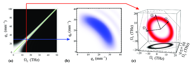
Figure 1: (a) Function sinc${}^{2}\left[\Delta k_{z}(q_{\Sigma},\Omega_{\Sigma})l/2\right]$ and corresponding spectral distributions in $q_{A}-q_{B}$ parameters (b) and in $\Omega_{A}-\Omega_{B}$ parameters (c) for type-I TOSPDC. Green dotted line in (a) corresponds to the phase-matching curve defined by the equation $\Delta k_{z}(q_{\Sigma},\Omega_{\Sigma})=0$. Calculation is made for 10 cm long rutile crystal at pump wavelength 532 nm.

In the biphoton case one can calculate the total count rate, integrating along the phase-matching curve, defined by the equation $\Delta k_{z}(q_{1},q_{2}=-q_{1},\Omega_{1},\Omega_{2}=-\Omega_{1})=0$. This case is comparatively simple as there are only two independent integration variables. Below we will derive the expressions for the curves analogous to the biphoton phase-matching curve in the case of triplets for the type-I and type-II TOSPDC collinear degenerate regime of generation.

In order to do this, let us expand $\Delta k_{z}$ in powers of $\Omega_{i}$, $q_{ix}$ and $q_{iy}$ up to the second order:

$${\color[rgb]{0,0,0}k_{z_{i}}=\sqrt{k_{i}^{2}-q_{i}^{2}},\quad k_{i}=n(\omega_{i})\frac{\omega_{i}}{c},\quad i=1,2,3},$$ (12)

$$\Delta k_{z}=k_{z1}+k_{z2}+k_{z3}-k_{p}=\left[k_{1}+k_{2}+k_{3}\right]_{0}-k_{p}+$$

$$\hphantom{\Delta_{z}}\sum\limits_{i=1,2,3}\left[\frac{\partial k_{i}}{\partial q_{ix}}\right]_{0}q_{ix}+\left[\frac{\partial k_{i}}{\partial q_{iy}}\right]_{0}q_{iy}+\left[\frac{\partial k_{i}}{\partial\omega_{i}}\right]_{0}\Omega_{i}+$$

$$\hphantom{\Delta_{z}}\frac{1}{2}\left[\frac{\partial^{2}k_{i}}{\partial q_{ix}^{2}}\right]_{0}q_{ix}^{2}+\frac{1}{2}\left[\frac{\partial^{2}k_{i}}{\partial q_{iy}^{2}}\right]_{0}q_{iy}^{2}+\frac{1}{2}\left[\frac{\partial^{2}k_{i}}{\partial\omega_{i}^{2}}\right]_{0}\Omega_{i}^{2}$$ (13)

Here $[\ldots]_{0}$ means that the expression in brackets is evaluated at the exact collinear degenerate regime of generation. All mixed derivatives are equal zero.

Let’s consider separately two types of phase-matching, type-I and type-II.

2.1 Type-I phasematching

In the case of phase matching of the type-I (e$\rightarrow$ooo) the first-order derivatives of $k_{i}$ in Eq. (12) appear to be identical for different $i$ and, as $\sum\limits_{i}q_{ix,y}=0$ and $\sum\limits_{i}\Omega_{i}=0$, Eq. (13) takes the form

$$\Delta k_{z}(q_{\Sigma},\Omega_{\Sigma})=\beta\Omega_{\Sigma}^{2}-\alpha q_{\Sigma}^{2},$$ (14)

where

$$\alpha=-\frac{1}{2}\left[\frac{\partial^{2}\Delta k_{z}}{\partial q_{i}^{2}}\right]_{0}=\frac{3}{2}k_{p},$$

$$\beta=\frac{1}{2}\left[\frac{\partial^{2}\Delta k_{z}}{\partial\omega_{i}^{2}}\right]_{0}=\frac{1}{4\pi c^{2}}\left[\lambda^{3}\frac{\partial^{2}n_{i}}{\partial\lambda_{i}^{2}}\right]_{0},$$

$$q_{\Sigma}^{2}=\sum\limits_{i=1,2,3}q_{i}^{2},\quad\Omega_{\Sigma}^{2}=\sum\limits_{i=1,2,3}\Omega_{i}^{2}.$$

Thus, $\Delta k_{z}$ depends on two variables, $q_{\Sigma}$ and $\Omega_{\Sigma}$, and hence, the exact-phase-matching curve is defined by the equation $\beta\Omega_{\Sigma}^{2}-\alpha q_{\Sigma}^{2}=0$ (the dotted green line in Fig. 1a).

Now, let us change the integration variables in Eq. (11) $\Omega_{1}$, $\Omega_{2}$, $\Omega_{3}$ $\rightarrow$ $\Omega_{A}$, $\Omega_{B}$, $\Omega_{C}$ (Fig. 1c):

$$\Omega_{A}=\frac{2\Omega_{3}-\Omega_{1}-\Omega_{2}}{\sqrt{6}},\quad\Omega_{B}=\frac{{\color[rgb]{0,0,0}\Omega}_{1}+{\color[rgb]{0,0,0}\Omega}_{2}}{\sqrt{2}},$$

$$\Omega_{C}=\frac{\Omega_{1}+\Omega_{2}+\Omega_{3}}{\sqrt{3}}$$

and $\vec{q}_{1}$, $\vec{q}_{2}$, $\vec{q}_{3}$ $\rightarrow$ $\vec{q}_{A}$, $\vec{q}_{B}$, $\vec{q}_{C}$:

$$\vec{q}_{A}=\frac{2\vec{q}_{3}-\vec{q}_{1}-\vec{q}_{2}}{\sqrt{6}},\quad\vec{q}_{B}=\frac{\vec{q}_{1}+\vec{q}_{2}}{\sqrt{2}},$$

$$\vec{q}_{C}=\frac{\vec{q}_{1}+\vec{q}_{2}+\vec{q}_{3}}{\sqrt{3}}.$$

In these variables $\delta(\Omega)\equiv\delta(\Omega_{C})$ and $\delta^{(2)}(\vec{q})\equiv\delta^{(2)}(\vec{q}_{C})$ in (11), owing to which integrals over $\Omega_{C}$ and $\vec{q}_{C}$ are easily taken. As for the other variables, let us introduce the polar coordinates in the planes $(q_{Ax},q_{Ay})$, $(q_{Bx},q_{By})$, $(q_{A},q_{B})$, and $(\Omega_{A},\Omega_{B})$:

$$q_{Ax}=q_{A}\cos{\phi_{A}},\quad q_{Ay}=q_{A}\sin{\phi_{A}},$$

$$q_{Bx}=q_{B}\cos{\phi_{B}},\quad q_{By}=q_{B}\sin{\phi_{B}},$$

$${q}_{A}=q_{\Sigma}\cos{\phi_{q}},\quad q_{B}=q_{\Sigma}\sin{\phi_{q}},$$

$$\Omega_{A}=\Omega_{\Sigma}\cos{\phi_{\Omega}},\quad \Omega_{B}=\Omega_{\Sigma}\sin{\phi_{\Omega}}.$$

The Jacobian of transformation to polar coordinates is given by $J=\Omega_{\Sigma}q_{\Sigma}^{3}\cos{\phi_{q}}\sin{\phi_{q}}$ and Eq. (11) takes the form:

$$I=\int dq_{\Sigma}d\Omega_{\Sigma}d\phi_{q}d\phi_{A}d\phi_{B}d\phi_{\Omega}\,J\,\mbox{sinc}^{2}\left(\frac{\Delta k_{z}l}{2}\right)=$$

$$\hphantom{I=}\frac{(2\pi)^{3}}{2}\int q_{\Sigma}^{3}dq_{\Sigma}\Omega_{\Sigma}d\Omega_{\Sigma}\,\mbox{sinc}^{2}\left(\frac{\Delta k_{z}l}{2}\right)$$ (15)

The phase-matching area in the plane ($\Omega_{\Sigma},q_{\Sigma}$) is shown in white in Fig. 1a. Each point at the exact-phase-matching curve in this area corresponds to one quarter of a ring of the spectral distribution in $q_{A}-q_{B}$ variables (Fig. 1b), and to a full ring of the distribution in the $\Omega_{A}-\Omega_{B}$ variables (Fig. 1c).The integrals over the $q_{A}-q_{B}$ and $\Omega_{A}-\Omega_{B}$ distributions are included into the Jacobian $J$.

The integral over $q_{\Sigma}$ in Eq. (15) can be approximated by the product of the integrand at the exact-phase-matching curve with the width of the phase-matching area in the $q_{\Sigma}$ direction, $\Delta q_{\Sigma}$. The latter can be found from the equation :

$$(\beta\Omega_{\Sigma}^{2}-\alpha(q_{\Sigma}+\Delta q_{\Sigma})^{2})l/2=\pi\;\Rightarrow\;q_{\Sigma}\,\Delta q_{\Sigma}=\frac{\pi}{l\alpha},$$ (16)

which reduces Eq. (15) to the form

$$I{\approx}\frac{(2\pi)^{3}}{2}\int\limits_{0}^{\Omega_{\Sigma max}}\frac{\pi}{\alpha l}\frac{\beta}{\alpha}\Omega_{\Sigma}^{3}d\Omega_{\Sigma}=\frac{\pi^{4}\beta}{\alpha^{2}l}\Omega^{4}_{\Sigma max},$$ (17)

where

$$\Omega_{\Sigma max}\equiv\min\left[\frac{2\pi c}{\lambda_{min}}-\frac{\omega_{p}}{3},\frac{\omega_{p}}{3}-\frac{2\pi c}{\lambda_{max}},\frac{k_{p}\theta_{max}}{3}\sqrt{\frac{\alpha}{\beta}}\right]$$

Here we have taken into account the limitation of the spectral (from $\lambda_{min}$ to $\lambda_{max}$) and angular (no more than $\theta_{max}$) detection range.

2.2 Type-II phasematching

Let us consider now the TOSPDC process with the type-II (e$\rightarrow$ooe) phase-matching. Let the optical axis of a crystal is located in the $(xz)$ plane. In this case the first-order derivatives in Eq. (13) are not equal and the decomposition of $\Delta k_{z}$ has the following form (we assume that the photons 1 and 2 are ordinary and the photon 3 is extraordinary):

$$\Delta k_{z}=\beta_{o}(\Omega_{1}+\Omega_{2})+\beta_{e}\Omega_{3}+\alpha_{e}q_{3x}+$$

$${\color[rgb]{0,0,0}\hphantom{qqqqqqqqqqqqqq}\frac{1}{2}\gamma_{ox}(q_{1x}^{2}+q_{2x}^{2})+\frac{1}{2}\gamma_{ex}q^{2}_{3x}+}$$

$$\hphantom{qqqqqqqqqqqqqq}\frac{1}{2}\gamma_{oy}(q_{1y}^{2}+q_{2y}^{2})+\frac{1}{2}\gamma_{ey}q^{2}_{3y},$$ (18)

where

$$\beta_{o}\equiv\frac{\partial k_{1,2}}{\partial\omega_{1,2}},\quad\beta_{e}\equiv\frac{\partial k_{3}}{\partial\omega_{3}},\quad\alpha_{e}\equiv\frac{\partial k_{3}}{\partial q_{3x}},$$

$$\gamma_{ox,y}\equiv\frac{\partial^{2}k_{1,2}}{\partial^{2}q_{1,2,x,y}},\quad\gamma_{ex,y}\equiv\frac{\partial^{2}k_{3}}{\partial^{2}q_{3,x,y}}.$$

We took into account here that inside a small angular range in the $x$-direction the terms with the second-order derivatives $\gamma_{o,ex}$ are much smaller than the terms with the first-order derivatives $\alpha_{o,e}$, but in the $y$-direction $\partial\Delta k_{z}/\partial q_{iy}$=0 and, hence, the second-order derivatives $\gamma_{o,ey}$ have to be retained.

By denoting $\gamma\simeq\gamma_{ey}\simeq\gamma_{oy}$, we get

$$\Delta k_{z}=(\beta_{o}-\beta_{e})(\Omega_{1}+\Omega_{2})-\alpha_{e}(q_{1x}+q_{2x})+$$

$$\gamma(q_{1y}^{2}+q_{2y}^{2}),$$ (19)

and the integral $I$ of Eq. (11) takes the form

$$I=\frac{2\pi}{l|\gamma|}\int\mbox{sinc}^{2}\left(\frac{[\beta_{+}\Omega_{+}-\alpha_{+}q_{+}]l}{2}\right)d\Omega_{+}d\Omega_{-}dq_{+}dq_{-},$$

where

$$\Omega_{\pm}=\frac{\Omega_{1}\pm\Omega_{2}}{\sqrt{2}},\quad q_{\pm}=\frac{q_{1x}\pm q_{2x}}{\sqrt{2}},$$

$$\alpha_{+}=\sqrt{2}\alpha_{e},\quad\beta_{+}=\sqrt{2}(\beta_{o}-\beta_{e}),$$

with the intervals of $q_{1,2y}^{2}$ where $\left|\Delta k_{z}l\right|<2\pi$ estimated as $\Delta q_{y}^{2}={2\pi}/{l|\gamma|}$.

Hence, the exact-phase-matching curve for type-II TOSPDC has the form $\beta_{+}\Omega_{+}-\alpha_{+}q_{+}=0$ (the green dotted line in Fig. 2a). Each point of the phase-matching area $\{\Omega_{+},q_{+}\}$ corresponds to the ranges $\Delta q_{-}$ (Fig. 2b) and $\Delta\Omega_{-}$ (Fig. 2c),

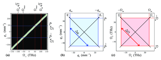
Figure 2: (a) The function sinc${}^{2}\left[{\Delta k_{z}(\Omega_{+},q_{+})}l/2\right]$ and the integration areas over the variables $q_{1}$, $q_{2}$ (b) and over the variables $\Omega_{1}$, $\Omega_{2}$ (c) for type-II TOSPDC. Green dotted line in (a) corresponds to the phase-matching curve defined by the equation $\Delta k_{z}(\Omega_{+},q_{+})=0$. Calculation is made for a 1 mm long calcite crystal at the pump wavelength 532 nm.

which can be found from phase-matching conditions:

$$\Delta q_{-}=2(q_{m}\sqrt{2}-|q_{+}|)=2\left(q_{m}\sqrt{2}-\left|\frac{\beta_{+}}{\alpha_{+}}\Omega_{+}\right|\right)$$

$$\hphantom{qqqqqqqqqqq}\mbox{(shown as blue arrow on Fig.\leavevmode\nobreak\ {\ref{fig:type_II}b})},$$

$$\Delta\Omega_{-}=2({\Omega}_{m}\sqrt{2}-|\Omega_{+}|)$$

$$\hphantom{qqqqqqqqqqqq}\mbox{(shown as red arrow on Fig.\leavevmode\nobreak\ {\ref{fig:type_II}c})}{.}$$

Similarly to the type-I case we approximate the integral over $q_{+}$ by the product of the integrand at the exact-phase-matching curve with the width of the phase-matching area $\Delta q_{+}=4\pi/|\alpha_{e}|l$ and get

$$I{\approx}\frac{2\pi}{l|\gamma|}\int\limits_{-\sqrt{2}\Omega_{max}}^{\sqrt{2}\Omega_{max}}d\Omega_{+}\cdot\Delta\Omega_{-}\Delta q_{+}\Delta q_{-}=$$

$$\frac{32\pi^{2}}{|\alpha_{e}\gamma|l^{2}}\int\limits_{-\sqrt{2}\Omega_{max}}^{\sqrt{2}\Omega_{max}}d\Omega_{+}\cdot({\Omega}_{m}\sqrt{2}-|\Omega_{+}|)\times$$

$$\hphantom{qqqqqqqqqqqqqqqq}\left(q_{m}\sqrt{2}-\left|\frac{\beta_{+}}{\alpha_{+}}\Omega_{+}\right|\right),$$ (20)

where $\Omega_{max}$, $\Omega_{m}$ and $q_{m}$ are determined by detection ranges in frequency and angle shown in Fig. 2:

$$q_{m}=k_{p}\theta_{max},\quad\Omega_{max}\equiv\min[{\Omega_{m}},\Omega_{q}],\quad\mbox{ {with}}$$

$${\Omega_{m}}\equiv\min\left[\frac{2\pi c}{\lambda_{min}}-\frac{\omega_{p}}{3},\frac{\omega_{p}}{3}-\frac{2\pi c}{\lambda_{max}}\right],\quad\Omega_{q}\equiv q_{m}{\frac{\alpha_{+}}{\beta_{+}}}.$$

.

3 Evaluation of the measurement time

The measurement time $T_{3}$ can be defined as the time sufficient for extracting the signal triple coincidence count rate $R_{s}^{(3)}$ from noise $R_{n}^{(3)}$. Mathematically this means that the total number of triple coincidence counts (found as the difference of two measured rates, of the sum of signal and noise counts and, separately, of only noise counts) $N_{s}^{(3)}=R_{s}^{(3)}T_{3}$ is at least $t_{C,\infty}$ times bigger than its standard deviation $\sigma_{s}^{(3)}$, where $t_{C,\infty}$ is the Student’s $t$-factor for a confidence level $C$. Taking into account the Poisson distribution of photo counts one can calculate the dispersions:

$$\sigma^{(3)}_{n}=\sqrt{R_{n}^{(3)}T_{3}},\quad\sigma^{(3)}_{n+s}=\sqrt{\left(R_{n}^{(3)}+R_{s}^{(3)}\right)T_{3}}$$

$$\sigma^{(3)}_{s}=\sqrt{\left(\sigma^{(3)}_{n}\right)^{2}+\left(\sigma^{(3)}_{n+s}\right)^{2}}=\sqrt{\left(2R_{n}^{(3)}+R_{s}^{(3)}\right)T_{3}}$$

So, we obtain the equation for $T_{3}$:

$${N^{(3)}=}T_{3}R_{s}^{(3)}={t_{C,\infty}}{\sigma_{s}^{(3)}}={t_{C,\infty}}\sqrt{\left(2R_{n}^{(3)}+R_{s}^{(3)}\right)T_{3}}.$$

With given quantum efficiency $\eta$ and the noise count rate $R_{n}^{(1)}$ of each detector¹ (we assume that all detectors have approximately the same characteristics), the temporal resolution of electronics (typically limited by a detector jitter) $\delta\tau$, and $R_{T}$ evaluated in (10), we get

$$R_{n}^{(3)}=\left(R_{n}^{(1)}\right)^{3}\delta\tau^{2},$$ (21)

$$R_{s}^{(3)}=\xi_{3}R_{T}\eta^{3},$$ (22)

where the parameter $\xi_{3}$ (and also the parameter $\xi_{2}$ – see below) characterizes features of non-polarized beam splitters to be used in a possible experimental setup for dividing TOSPDC signal into three channels. Hence,

$$T_{3}={t_{C,\infty}^{2}}\frac{2\left(R_{n}^{(1)}\right)^{3}\delta\tau^{2}+\xi_{3}R_{T}\eta^{3}}{\left(\xi_{3}R_{T}\eta^{3}\right)^{2}}.$$ (23)

Similar expressions can be derived for the minimal time $T_{2}$ ($T_{1}$) required for distinguishing two-photon signal coincidence and single-photon counts from the noise:

$$T_{2}={t_{C,\infty}^{2}}\frac{2\left(R_{n}^{(1)}\right)^{2}\delta\tau+\xi_{2}R_{T}\eta^{2}}{\left(\xi_{2}R_{T}\eta^{2}\right)^{2}},$$ (24)

$$T_{1}={t_{C,\infty}^{2}}\frac{2R_{n}^{(1)}\delta\tau+R_{T}\eta}{\left(R_{T}\eta\right)^{2}}$$ (25)

and in case of two consistent 30/70 and 50/50 beam splitters, which provide approximately equal power in three channels, parameters $\xi_{3,2}$ are given by $\xi_{3}=0.22$ and $\xi_{2}=0.75$.

4 Example: calcite and rutile crystals

Let us make estimates for two specific crystals, calcite and rutile, having comparatively large cubic susceptibilities. For these two crystals and for four pump wavelengths, 266, 325, 405 and 532 nm, the results of calculations are presented in Table 1. By using data about crystal refractive indices of Refs. [26, 27], we found values of angles between the optical axes of crystals and the pump propagation direction providing collinear emission of TOSPDC photons. For these orientations of crystals, with the use of matrix elements determining $\chi^{(3)}$ [28, 29, 30, 31], and with the dependence of $\chi^{(3)}$ on the angle between the pump propagation direction and the crystal optical axis [32] taken into account, we calculated values of the effective cubic susceptibility $\chi^{(3)}_{eff}$ for both crystals and for all collinear TOSPDC regimes indicated in Table 1. Together with $\chi^{(3)}_{eff}$, we present in Table 1 the total count rates (10), calculated from Eq. (17) for rutile and from Eq. (2.2) for calcite.

Table 1: Calculated values of effective third-order nonlinear susceptibility $\chi^{(3)}_{eff}$, triplets generation rates $R_{T}$, measurement times necessary for registration of triple $T_{3}$ and double $T_{2}$ coincidences for different pump wavelengths $\lambda_{p}$ and power $W_{p}$, type of nonlinear media, its length $l$ and type of phase-matching, for different detectors and for the cases with presence $(+)$ and absence $(-)$ the cavity. Easy accessible in an experiment values marked as green, hardly accessible as yellow and unaccessible as red.

$\lambda_{p}$	Medium	$\chi^{(3)}_{eff}$	$W_{p}$,	Detector	l	Cavity	$R_{T}$	$T_{3}$	$T_{2}$
(nm)		$(10^{-15}$esu)	(W)		(mm)		(Hz)	(days)	(days)
266	Calcite	0.32	10	Si APD	0.1	$-$	$4.0\cdot 10^{-5}$	94	15
	(e$\rightarrow$ooe)					$+$	$4.0\cdot 10^{-2}$	$9.4\cdot 10^{-2}$	$1.4\cdot 10^{-2}$
325	Calcite	0.59	0.05	Si APD	0.1	$+$	$1.1\cdot 10^{-5}$	5 200	750
	(e$\rightarrow$ooe)			Super Cond.			$3.4\cdot 10^{-6}$	18 000	1 000
405	Calcite	0.76	0.5	PMD	0.1	$+$	$1.8\cdot 10^{-4}$	$8.1\cdot 10^{10}$	$2.0\cdot 10^{11}$
	(e$\rightarrow$ooe)			Super Cond.			$9.5\cdot 10^{-6}$	6 200	$370$
532	Calcite	0.88	10	PMD	0.1	$+$	$1.8\cdot 10^{-4}$	$8.2\cdot 10^{10}$	$2.0\cdot 10^{11}$
	(e$\rightarrow$ooe)			Super Cond.			$5.0\cdot 10^{-6}$	1 200	$690$
532	Rutile	71.6	10	PMD	100	$-$	$1.5\cdot 10^{-2}$	$1.1\cdot 10^{7}$	$2.8\cdot 10^{7}$
	(o$\rightarrow$eee)			Super Cond.	0.77		$8.9\cdot 10^{-7}$	$6.6\cdot 10^{4}$	$3.9\cdot 10^{3}$

Note that though rutile is a positive crystal and in the type-I phase-matching all three TOSPDC photons are not ordinary, it can be shown that even in this case the calculation based on (17) results in inaccuracy of $\Delta k_{z}$ about 10 percents.

The phase-matching conditions in calcite at the mentioned pump wavelengths are satisfied for each type of phase-matching (e$\rightarrow$ooo, e$\rightarrow$ooe and e$\rightarrow$oee), but for all types except e$\rightarrow$ooe values of $\chi^{(3)}_{eff}$ are very small and, therefore, these cases are not included into Table 1.

We paid special attention to calculations of the optimal crystal length $l$ and angular detection range $\theta_{max}$ .

Note, first, that the total count rate is proportional to $l$ in type-I (8), (17) and independent of $l$ in type-II (8), (2.2) phase-matching cases. The last assertion is correct while in the phase-matching inequality (see (2.2) and further)

$$|\Delta k_{z}|=\left|\alpha q+\frac{1}{2}\gamma q^{2}\right|<\frac{2\pi}{l}$$

the quadratic term can be omitted. For calcite this is true for $l\gg l_{min}=4\pi\gamma/\alpha^{2}\sim 0.05$ mm . But the crystal length can limit the detection angular range. For multi-mode detection (see Table 2) we assume $\theta_{max}=\pi/2$² (we suppose, that all the SPDC radiation can be focused on the detector area). But for single-mode detection the angular range is defined by a gaussian mode divergence $\theta_{max}=\lambda/\pi w$, where $w$ is the waist of the pump, which should be less than the spatial walk-off $\rho l$ (for the considered crystals $\rho\sim 0.1$). So, we obtain $\theta_{max}\propto 1/l$. It means that in the case of type-II phase-matching we need to use as thin crystal as possible (we set $l=2l_{min}=0.1$ mm). In the case of type-I phase-matching the crystal length $l$ has to be decreased until the integration limits in Eq. (17) become defined by the angular range. This means that the optimal crystal length is

$$l=\frac{k_{p}\lambda}{3\pi\rho}\sqrt{\frac{\alpha}{\beta}}\left/\min\left[\frac{2\pi c}{\lambda_{min}}-\frac{\omega_{p}}{3},\frac{\omega_{p}}{3}-\frac{2\pi c}{\lambda_{max}}\right]\right..$$

Finally, for multi-mode detection and the type-I phase-matching the crystal has to be taken as long as possible (we set 100 mm).

[b] Type $\lambda_{min}$-$\lambda_{max}$ Number Quantum Dark count rate $R_{n}^{(1)}$ Jitter $\delta\tau$ (nm) of spatial modes efficiency $\eta$ (Hz) (ps) Si APD¹ $\hphantom{1}400$–$1040$ Multi 0.1-0.7 100 350 InGaAs APD² $1000$–$1650$ Single 0.1 3000 200 Super Conductive³ $\hphantom{1}600$–$1700$ Single 0.2 1 50 PMD⁴ $\hphantom{1}950$–$1700$ Multi 0.01 50000 70

Table 2: Characteristics of single-photon detectors to be used for three-photons registration.

• Excelitas SPCM-AQRH-16

• IDQuantique ID210

• Scontel SSPD

• Hamamatsu R3809U-69

5 Results and Discussion

In calculations we took parameters of the most widely used single-photon detectors (see Table 2) and the most suitable cw lasers: DPSS lasers at 266 and 532 nm, diode blue-ray laser at 405 nm and HeCd gas laser at 325 nm. Typical powers are given in Table 1. It was shown[22] that the use of pulsed pump lasers gives no advantages for TOSPDC generation.

Also we consider a possibility of increasing the pump power inside the crystal by means of mirror deposition at the rear and front faces of the crystal, which turns the latter into a cavity. Accordingly, maximal growth of the pump intensity in a crystal (cavity) is characterized by the factor $\varepsilon=$1000.³ Unfortunately, this optimization cannot be used in rutile crystals because of their comparatively high adsorption.

In addition to the total triplet generation rates $R_{T}$, we have calculated and presented in Table 1 the time, required for two- and three-photon coincidences, (23) and (24) at $t_{0.998,\infty}=3$. .

One can see, that one of the main problems of TOSPDC detection is related to low efficiency and high noise of IR detectors. It is really difficult to extract a signal from noise even for triple coincidence measurements. So we found only one combination of parameters when detection of TOSPDC photons looks possible. This is the case of a calcite crystal with a mirror coverage deposited at rear and front faces, the crystal length $l=0.1$ mm, and the pump parameters $\lambda_{p}$=266 nm and $W_{p}$=10 W. In this case we found $T_{2}=20$ and $T_{3}=135$ minutes.

One more advantage of UV pump is the increase of the differential generation rate, because it is proportional to $\omega_{1}\omega_{2}\omega_{3}\propto\omega_{p}^{3}$ (8).

Another well-known problem is a low value of $\chi^{(3)}_{eff}$. For rutile crystal $\chi^{(3)}_{eff}$ is about two orders higher if the crystal optical axis is taken parallel to the pump propagation direction. But for the phase-matching conditions to be satisfied one has to use a crystal with periodical poling (quasi-phase-matching). This is an evident way for making the type-I and type-II phase-matching conditions satisfied and TOSPDC photons detectable in visible range of wavelengths. Another possibility of increasing $\chi^{(3)}_{eff}$ is an addition of special impurities to crystals which would provide resonance enhancement of the third-order susceptibility.

One more problem is a really multi-mode structure of TOPDC generation in bulk crystals, which requires multi-mode detection of signals. This problem can be solved by producing a wave-guide inside the crystal medium, as proposed in [34]. In this way the length of interaction can be done arbitrary long.

6 Conclusion

Finally, we have performed a detailed analysis of three-photon generation in birefringent crystals with special attention paid to calcite and rutile crystals. The analysis includes the calculation of differential generation rate in unit frequency and transverse wave vectors range (8), total count rate (10) for type-I and type-II phase-matching and measurement time, required for distinguishing signal coincidences from noise ((24) and (23)).

The results show that the registration of TOSPDC in calcite is possible for the process with the pump at 266 nm with the presence of a cavity. All the other considered cases need too much time for three-photon registration.

This work was supported by the Russian Science Foundation (project 14-12-01338).

7 References

References

- [1] Cezary Śliwa and Konrad Banaszek. Conditional preparation of maximal polarization entanglement. Physical Review A, 67(3):030101, March 2003.
- [2] Stefanie Barz, Gunther Cronenberg, Anton Zeilinger, and Philip Walther. Heralded generation of entangled photon pairs. Nature Photonics, 4(8):553–556, August 2010.
- [3] Claudia Wagenknecht, Che-Ming Li, Andreas Reingruber, Xiao-Hui Bao, Alexander Goebel, Yu-Ao Chen, Qiang Zhang, Kai Chen, and Jian-Wei Pan. Experimental demonstration of a heralded entanglement source. Nature Photonics, 4(8):549–552, August 2010.
- [4] Anton Zeilinger, A Horne, and Daniel M Greenberger. Higher-Order Quantum Entanglement. NASA Conf. Publ., (3135):73–81, 1992.
- [5] Dik Bouwmeester, Jian-Wei Pan, Matthew Daniell, Harald Weinfurter, and Anton Zeilinger. Observation of Three-Photon Greenberger-Horne-Zeilinger Entanglement. Physical Review Letters, 82(7), 1999.
- [6] Timothy E Keller, Morton H Rubin, and Yanhua Shih. Theory of the three-photon entangled state. phys rev a, 57(3), 1998.
- [7] Hannes Hübel, Deny R Hamel, Alessandro Fedrizzi, Sven Ramelow, Kevin J Resch, and Thomas Jennewein. Direct generation of photon triplets using cascaded photon-pair sources. Nature, 466(7306):601–603, 2010.
- [8] L K Shalm, D R Hamel, Z Yan, C Simon, K J Resch, and T Jennewein. Three-photon energy – time entanglement. Nature Physics, 9(1):19–22, 2012.
- [9] Mitsuyoshi Yukawa, Kazunori Miyata, Takahiro Mizuta, Hidehiro Yonezawa, Petr Marek, Radim Filip, and Akira Furusawa. Generating superposition of up-to three photons for continuous variable quantum information processing. Optics Express, 21(5):5, 2013.
- [10] Deny R. Hamel, Lynden K. Shalm, Hannes Hübel, Aaron J. Miller, Francesco Marsili, Varun B. Verma, Richard P. Mirin, Sae Woo Nam, Kevin J. Resch, and Thomas Jennewein. Direct generation of three-photon polarization entanglement. Nature Photonics, 8(10):801–807, September 2014.
- [11] T. Guerreiro, A. Martin, B. Sanguinetti, J. S. Pelc, C. Langrock, M. M. Fejer, N. Gisin, H. Zbinden, N. Sangouard, and R. T. Thew. Nonlinear Interaction between Single Photons. Physical Review Letters, 113(17):173601, 2014.
- [12] Stephan Krapick, Benjamin Brecht, Viktor Quiring, Raimund Ricken, Harald Herrmann, and Christine Silberhorn. On-Chip generation of photon-triplet states in integrated waveguide structures. In CLEO: 2015, page FM2E.3, Washington, D.C., May 2015. OSA.
- [13] J. Rarity and P. Tapster. Three-particle entanglement from entangled photon pairs and a weak coherent state. Physical Review A, 59(1):R35–R38, 1999.
- [14] J Douady and B Boulanger. Experimental demonstration of a pure third-order optical parametric downconversion process. Optics letters, 29(23), 2004.
- [15] Fabien Gravier and Benoît Boulanger. Triple-photon generation: comparison between theory and experiment. Journal of the Optical Society of America B, 25(1):98, 2008.
- [16] M. V. Chekhova, O. a. Ivanova, V. Berardi, and A. Garuccio. Spectral properties of three-photon entangled states generated via three-photon parametric down-conversion in a medium. Physical Review A, 72(2):23818, 2005.
- [17] Kamel Bencheikh, Fabien Gravier, Julien Douady, Ariel Levenson, and Benoît Boulanger. Triple photons: a challenge in nonlinear and quantum optics. Comptes Rendus Physique, 8(2):206–220, 2007.
- [18] A Dot, A Borne, B Boulanger, K Bencheikh, and J A Levenson. Quantum theory analysis of triple photons generated by a process. Physical Review A, 85(2):023809, February 2012.
- [19] S Richard, K Bencheikh, B Boulanger, and J A Levenson. Semiclassical model of triple photons generation in optical fibers. Opt. Lett., 36(15):3000–3002, 2011.
- [20] Karol Tarnowski, Bertrand Kibler, Christophe Finot, and Waclaw Urbanczyk. Quasi-phase-matched third harmonic generation in optical fibers using refractive-index gratings. IEEE Journal of Quantum Electronics, 47(5):622–629, 2011.
- [21] María Corona, Karina Garay-palmett, and Alfred B U Ren. Experimental proposal for the generation of entangled photon triplets by third-order spontaneous parametric downconversion in optical fibers. Opt. Lett., 36(2):190–192, 2011.
- [22] María Corona, Karina Garay-Palmett, and Alfred B. U’Ren. Third-order spontaneous parametric down-conversion in thin optical fibers as a photon-triplet source. Physical Review A - Atomic, Molecular, and Optical Physics, 84(3):1–13, 2011.
- [23] Tianye Huang, Zhifang Wu, Xuguang Shao, Jing Zhang, and Lam Quoc Huy. Generation photon triplets in mid-infrared by third order spontaneous parametric down conversion in micro-fiber. In Asia Communications and Photonics Conference 2013, page ATh3C.5, Beijing, China, 2013. Optical Society of America.
- [24] Tianye Huang, Xuguang Shao, Zhifang Wu, Timothy Lee, Yunxu Sun, Huy Quoc Lam, Jing Zhang, Gilberto Brambilla, and Shum Ping. Efficient one-third harmonic generation in highly Germania-doped fibers enhanced by pump attenuation. Optics Express, 21(23):28403, November 2013.
- [25] David Nikolaevich Klyshko. Photons and nonlinear optics. Gordon and Breach, New York, 1988.
- [26] Gorachand Ghosh. Dispersion-equation coefficients for the refractive index and birefringence of calcite and quartz crystals. Optics Communications, 163(1-3):95–102, 1999.
- [27] Fabien Gravier and Benoît Boulanger. Cubic parametric frequency generation in rutile single crystal. Optics express, 14(24):11715–11720, 2006.
- [28] N.G. Khadzhiiski and N.I. Koroteev. Coherent Raman ellipsometry of crystals: Determination of the components and the dispersion of the third-order nonlinear susceptibility tensor of rutile. Optics Communications, 42(6):423–427, August 1982.
- [29] M Thalhammer and A Penzkofer. Measurement of Third-Order Nonlinear Susceptibilities by Non Phase Matched Third-Harmonic Generation. Applied Physics B, 143(32):137–143, 1983.
- [30] A Penzkofer, F Ossig, and P Qiu. Picosecond third-harmonic light generation in calcite. Applied Physics B Photophysics and Laser Chemistry, 47(1):71–81, 1988.
- [31] Adrien Borne, Patricia Segonds, Benoit Boulanger, Corinne Félix, and Jérôme Debray. Refractive indices, phase-matching directions and third order nonlinear coefficients of rutile TiO2 from third harmonic generation. Optical Materials Express, 2(12):1797–1802, 2012.
- [32] J E Midwinter and J Warner. The effects of phase matching method and crystal symmetry on the polar dependence of third-order non-linear optical polarization. brit j appl phys, 16, 1965.
- [33] A E Siegman. Resonance Properties of Passive Optical Cavities. In Lasers, chapter 11, page 1283. University Science Books, Mill Valley, 1986.
- [34] Eric Mazur, Christopher Courtney Evans, Michael Gerhard Moebius, Orad Reshef, and Sarah E. Griesse-Nascimento. Direct Entangled Triplet-Photon Sources And Methods For Their Design And Fabrication (US20150117826 A1), April 2015.