Scalar and tensor perturbations in loop quantum cosmology: High-order corrections

Abstract

Loop quantum cosmology (LQC) provides promising resolutions to the trans-Planckian issue and initial singularity arising in the inflationary models of general relativity. In general, due to different quantization approaches, LQC involves two types of quantum corrections, the holonomy and inverse-volume, to both of the cosmological background evolution and perturbations. In this paper, using the third-order uniform asymptotic approximations, we derive explicitly the observational quantities of the slow-roll inflation in the framework of LQC with these quantum corrections. We calculate the power spectra, spectral indices, and running of the spectral indices for both scalar and tensor perturbations, whereby the tensor-to-scalar ratio is obtained. We expand all the observables at the time when the inflationary mode crosses the Hubble horizon. As the upper error bounds for the uniform asymptotic approximation at the third-order are $\lesssim 0.15\%$, these results represent the most accurate results obtained so far in the literature. It is also shown that with the inverse-volume corrections, both scalar and tensor spectra exhibit a deviation from the usual shape at large scales. Then, using the Planck, BAO and SN data we obtain new constraints on quantum gravitational effects from LQC corrections, and find that such effects could be within the detection of the forthcoming experiments.

I Introduction

The inflationary cosmology provides the simplest and most elegant mechanism to produce the primordial density perturbations and primordial gravitational waves (PGWs) Guth ; InfGR . The former grows to produce the large-scale structure (LSS) seen today in the universe, and meanwhile creates the cosmic microwave background (CMB) temperature anisotropy, which has been extensively probed by WMAP WMAP , PLANCK PLANCK , and other CMB experiments as well as galaxy surveys. PGWs, on the other hand, produce not only a temperature anisotropy, but also a distinguishable signature in CMB polarization–the B-mode, which was once thought to be already observed by BICEP2 BICEP2 , although subsequent analysis of multi-frequency data from BICEP2/Keck and Planck Collaborations showed that the signals could be due to galactic dust Planck-intermediate (see also Mort2014 ), and further confirmation is needed. These observations in the measurement of the power spectra and spectral indices, together with the forthcoming ones, provide unique opportunities for us to gain deep insight into the physics of the very early Universe. More importantly, they may provide a unique window to explore quantum gravitational effects, which otherwise cannot be studied in the near future by any man-made terrestrial experiments.

Inflation is very sensitive to Planckian physics DB . In particular, in most inflationary scenarios, the energy scale of the inflationary fluctuations, which relates to the present observations, was not far from the Planck scale at the beginning of inflation. As in such high energy regime the usual classical general relativity and effective field theory are known to be broken, and it is widely expected a quantum theory of gravity could provide a complete description of the early Universe. However, such a theory of quantum gravity has not been established yet, and only a few candidates exist. One of the promising approaches is loop quantum gravity. On the basis of this theory, loop quantum cosmology (LQC) was proposed, which offers a natural framework to address the trans-Planckian issue and initial singularity, arising in the inflation scenarios. In fact, in LQC, because of the quantum gravitational effects deep inside the Planck scale, the big bang singularity is replaced by a big bounce Bojowald2001 ; Ashtekar2006 . This remarkable feature has motivated a lot of interest to consider the underlying quantum geometry effects in the standard inflationary scenario and their detectability QGEs .

In LQC, roughly speaking, there are two kinds of quantum gravitational corrections to the cosmological background and cosmological perturbations: the holonomy Mielczarek2008 ; Grain2009PRL ; Grain2010PRD ; vector_holonomy ; scalar ; scalar2 ; loop_corrections and the inverse-volume Bojowald2008 ; Bojowald2009 ; Bojowald2007 ; Bojowald2008b ; Bojowald2011 ; Bojowald2011b . The main consequence of holonomy corrections on the cosmological background is to replace the big bang singularity of the Friedmann-Lemaître-Robertson-Walker (FLRW) universe by a big bounce. The cosmological scalar scalar , vector vector_holonomy , and tensor perturbations Mielczarek2008 ; Grain2009PRL ; Grain2010PRD have been calculated explicitly with holonomy corrections (see also scalar2 ). Due to these corrections, the modifications of the algebra of constraints generically leads to anomalies vector_holonomy ; scalar . Recently, it has been shown that these anomalies can be removed by adjusting the form of the quantum corrections to the Hamiltonian constraint. This is achieved by adding suitable counter terms that vanish in the classical limit vector_holonomy ; scalar ; scalar2 . With these anomaly-free cosmological perturbations, the dispersion relation of the inflationary mode function $\mu_{k}(\eta)$ (of scalar and tensor perturbations) is modified by the quantum corrections to the form scalar2 ; loop_corrections ,

$$\omega^{2}_{k}(\eta)=\left(1-2\frac{\rho(\eta)}{\rho_{c}}\right)k^{2},$$ (1.1)

where $\rho_{c}$ is the energy density at which the big bounce happens. In the classical limit $\rho\ll\rho_{c}$, the above equation reduces to the standard one of GR. From this equation, one can see that when the energy density $\rho$ approaches ${\rho_{c}}/{2}$, the dynamics of cosmological perturbations is significantly modified by the holonomy corrections. With this modified dispersion relation, the power spectra for both scalar and gravitational wave perturbations were calculated up to the first-order approximations of the slow-roll parameters, and the observability of these corresponding quantum gravitational effects were discussed in some detail loop_corrections ; Mielczarek2014 .

The inverse-volume corrections are due to terms in the Hamiltonian constraint which cannot be quantized directly but only after being re-expressed as a Poisson bracket. It was demonstrated that the algebra of cosmological scalar Bojowald2008 ; Bojowald2009 , vector Bojowald2007 , and tensor perturbations Bojowald2008b with quantum corrections can be closed. Consequently, the cosmological perturbed equations for scalar and tensor perturbations are modified Bojowald2011 ; Bojowald2011b . For the scalar perturbations, the dispersion relation takes the form Bojowald2011

$$\omega^{2}_{k}(\eta)=\left\{1+\left[\frac{\sigma\vartheta_{0}}{3}\left(\frac{\sigma}{6}+1\right)+\frac{\alpha_{0}}{2}\left(5-\frac{\sigma}{3}\right)\right]\delta_{\text{Pl}}(\eta)\right\}k^{2},$$

where the constants $\alpha_{0}$, $\vartheta_{0}$, and $\sigma$ encode the specific features of the model, and $\delta_{\text{Pl}}(\eta)$ is time-dependent, which usually behaves like $\delta_{\text{Pl}}\sim a^{-\sigma}$. For tensor perturbations, $\omega^{2}_{k}(\eta)$ is given by Bojowald2011 ,

$$\omega^{2}_{k}(\eta) = \Big{(}1+2\alpha_{0}\delta_{\text{Pl}}(\eta)\Big{)}k^{2}.$$ (1.3)

The power spectra of both scalar and tensor perturbations due to the inverse-volume corrections, again up to the first-order approximations of the slow-roll parameters, were studied in Bojowald2011 , in which some constraints on some parameters of the model were obtained from observational data Bojowald2011b . The non-Gaussianities with inverse-volume corrections was also discussed in Cai2012 .

Although a lot of effort has already been devoted to the inflationary models of LQC with both holonomy and inverse-volume quantum corrections, very accurate calculations of inflationary observables in LQC are still absent, and with the arrival of the era of precision cosmology, such calculations are highly demanded. Recently, we have developed a powerful method, the uniform asymptotic approximation method Zhu1 ; Zhu2 ; Uniform3 ; Uniform4 , to make precise observational predictions from inflation models, after quantum gravitational effects are taken into account. We note here that such method was first applied to inflationary cosmology in uniformPRL , and then we have developed it to more general mult-turning points cases and more precise higher order approximations Zhu1 ; Zhu2 ; Uniform3 ; Uniform4 . The main purpose of the present paper is to use this powerful method to derive the inflationary observables in LQC with holonomy and inverse-volume quantum corrections with high accuracy. More specifically, we consider the slow-roll inflation with the quantum gravitational corrections, but ignore the pre-inflation dynamics. By using the general expressions of power spectra, spectral indices, and running of spectral indices obtained in Uniform3 , we calculate explicitly these quantities, up to the third-order approximations in terms of the uniform asymptotic approximation parameter, for which the upper error bounds are $\lesssim 0.15\%$. All the inflationary observables are expressed in terms of slow-roll parameters and parameters representing quantum corrections explicitly. In the present paper, we also provide the expansion of all these inflationary observables at the time when the inflationary mode crosses the Hubble horizon, and calculate the tensor-to-scalar ratio. It is interesting to note that the holonomy corrections do not contribute to the tensor-to-scalar ratio up to the third-order approximation. More interestingly, it is shown that with the inverse-volume corrections, both scalar and tensor spectra exhibit a deviation from the standard one at large scales, which could provide a smoking gun for further observations.

The paper is organized as follows. In Sec. II, we present all the background evolution and perturbation equations with the holonomy corrections, and calculate explicitly the power spectra, spectral indices, and running of spectral indices. Then, in Sec. III we turn to consider both background and perturbations with the inverse-volume corrections, and calculate all the inflationary observables. Our main conclusions are summarized in Sec. IV. Three appendices are also included. In Appendix A, we give a brief introduction to the uniform asymptotic approximation method with high-order corrections, while in Appendices B and C, we present some quantities discussed in the content of the paper.

Part of the results to be presented in this paper was reported recently in Zhu3 . In this paper, we shall provide detailed derivations of these results, and meanwhile report our studies of other aspects of LQC inflationary cosmology.

II Inflationary observables with holonomy corrections

In this section, let us consider the inflationary cosmology with the holonomy corrections.

II.1 Background equations and equations of motion for scalar and tensor perturbations

To begin with, let us first consider a flat FLRW background

$$ds^{2}=a^{2}(\eta)(-d\eta^{2}+dx^{i}dx^{i}),$$ (2.1)

where $a(\eta)$ is the expansion factor and $\eta$ the conformal time. With the holonomy corrections, the Friedmann equation is modified to the form Ashtekar2006

$$H^{2}=\frac{8\pi G}{3}\rho\left(1-\frac{\rho}{\rho_{c}}\right),$$ (2.2)

where $H=\dot{a}/a$ is the Hubble parameter with a dot representing derivative with respect to the cosmic time $t$ ($dt\equiv ad\eta$), $\rho$ is the energy density of the matter content, and $\rho_{c}$ is a characteristic energy scale of the holonomy corrections and usually is of the order of the Planck energy density: $\rho_{c}\sim m_{\text{Pl}}^{4}$ with the Planck mass $m_{\text{Pl}}=1.22\times 10^{19}\text{GeV}$. A general prediction associated with the above equation is that the holonomy corrections lead to a resolution of the big bang singularity, in which it is replaced by a non-singular big bounce occurring at $\rho=\rho_{c}$. For a scalar field $\varphi$ with potential $V(\varphi)$, the Klein-Gordon equation reads

$$\ddot{\varphi}+3H\dot{\varphi}+\frac{dV(\varphi)}{d\varphi}=0.$$ (2.3)

The energy density of the inflaton field is

$$\rho=\frac{\dot{\varphi}^{2}}{2}+V(\varphi).$$ (2.4)

The above set of equations determines uniquely the evolution of the FLRW background. As shown in slow-roll-holonomy , “the standard slow-roll inflation” can be triggered by the preceding phase of quantum bounce. In this paper, for the sake of simplification, we shall focus on the slow-roll inflation with the holonomy corrections, and ignore the pre-inflation dynamics. In this case, we are in a process such that the energy density of the cosmological fluid is supposed to be dominated by the potential of inflaton $\varphi$, i.e., $\dot{\varphi}^{2}\ll V(\varphi)$. With this condition, it is convenient to define a hierarchy of Hubble flow parameters,

$$\epsilon_{0}\equiv\frac{H_{\text{ini}}}{H},\;\;\;\epsilon_{n+1}\equiv\frac{d\ln\epsilon_{n}}{d\ln a}.$$ (2.5)

On the other hand, as the quantum holonomy correction is also small, it is convenient to introduce the parameter $\delta_{H}$ by,

$$\delta_{H}\equiv\frac{\rho}{\rho_{c}}\ll 1.$$ (2.6)

Then we have $\Omega\equiv 1-2\rho/\rho_{c}=1-2\delta_{H}$.

Let us now consider cosmological perturbations. With the holonomy corrections, the equations for cosmological scalar perturbations can be cast in a modified Mukhanov equation for the gauge-invariant mode function $\mu_{k}^{(s)}(\eta)$ scalar ; scalar2 ,

$$\frac{d^{2}\mu_{k}^{(s)}(\eta)}{d\eta^{2}}+\left(\omega_{k}^{2}(\eta)-\frac{z_{s}^{\prime\prime}(\eta)}{z_{s}(\eta)}\right)\mu_{k}^{(s)}(\eta)=0,$$ (2.7)

where $\omega_{k}^{2}(\eta)=\Omega(\eta)k^{2}$, and $z_{s}\equiv a\dot{\varphi}/H$. Similarly, the equation for the tensor perturbation can be cast in the form scalar2 ,

$$\frac{d^{2}\mu_{k}^{(t)}(\eta)}{d\eta^{2}}+\left(\Omega(\eta)k^{2}-\frac{z_{t}^{\prime\prime}(\eta)}{z_{t}(\eta)}\right)\mu_{k}^{(t)}(\eta)=0,$$ (2.8)

where $z_{t}\equiv a/\sqrt{\Omega}$.

II.2 Power spectra and spectral indices in the uniform asymptotic approximation

To apply for the uniform asymptotic approximation, first we write the equations of motion for both scalar (Eq. (2.7)) and tensor (Eq. (2.8)) perturbations in the form (A.1) by introducing a new variable $y=-k\eta$. Then, we find that $\hat{g}(y)$ and $q(y)$ must be chosen as Zhu1 ; Zhu2 ,

$$\lambda^{2}\hat{g}(y) = -\frac{1}{k^{2}}\left(\Omega(\eta)-\frac{z^{\prime\prime}(\eta)}{z(\eta)}\right)+\frac{1}{4y^{2}}$$ (2.9)

$$= \frac{\nu^{2}(\eta)}{y^{2}}-c_{s}^{2}(\eta),$$

$$q(y) = -\frac{1}{4y^{2}},$$ (2.10)

where $c_{s}(\eta)=\sqrt{\Omega(\eta)}$ and $\nu^{2}(\eta)=\eta^{2}z^{\prime\prime}(\eta)/z(\eta)+1/4$. For the scalar perturbations, using the slow-roll parameters defined in Eqs. (2.5) and (2.6), we find that

$$\frac{z_{s}^{\prime\prime}(\eta)}{z_{s}(\eta)} \simeq a^{2}H^{2}\Big{(}2-\epsilon_{1}+\frac{3\epsilon_{2}}{2}+\frac{\epsilon_{2}^{2}}{4}+\frac{\epsilon_{2}\epsilon_{3}}{2}-\frac{\epsilon_{1}\epsilon_{2}}{2}$$

$$~{}~{}~{}-6\epsilon_{1}\delta_{H}+6\epsilon_{1}^{2}\delta_{H}-4\epsilon_{1}\epsilon_{2}\delta_{H}-18\epsilon_{1}\delta_{H}^{2}\Big{)}.$$

In the above, we used the subscript (or superscript) “s” to denote quantities associated with the scalar perturbations. Similarly, for the tensor perturbations, we find

$$\frac{z_{t}^{\prime\prime}(\eta)}{z_{t}(\eta)} \simeq a^{2}H^{2}\Big{(}2-\epsilon_{1}-6\delta_{H}\epsilon_{1}-18\delta_{H}^{2}\epsilon_{1}-48\delta_{H}^{3}\epsilon_{1}$$

$$~{}~{}+6\delta_{H}\epsilon_{1}^{2}+38\delta_{H}^{2}\epsilon_{1}^{2}-2\delta_{H}\epsilon_{1}\epsilon_{2}-6\delta_{H}^{2}\epsilon_{1}\epsilon_{2}\Big{)},$$

where the subscript (or superscript) “t” denotes quantities associated with the tensor perturbations.

With the functions $\hat{g}(y)$ and $q(y)$ given above, we are in the position to calculate the power spectra and spectral indices from the general formulas Eq. (B. Power spectra and spectral indices up to the third-order) and Eq. (A.27). As we discussed in Zhu2 , in order to do so, first we need to expand $\nu(\eta)$ and $c_{s}(\eta)$ around the turning point $\bar{y}_{0}$ of $\hat{g}(y)$ (i.e., $\hat{g}(\bar{y}_{0})=0$ with $\bar{y}_{0}=-k\eta_{0}$), then perform the integral of $\sqrt{\hat{g}(y)}$ in Eq. (B. Power spectra and spectral indices up to the third-order), and calculate the error control function $\mathscr{H}(+\infty)$. In the slow-roll inflation, it is convenient to consider the following expansions,

$$\nu(\eta) \simeq \bar{\nu}_{0}+\bar{\nu}_{1}\ln\frac{y}{\bar{y}_{0}}+\frac{1}{2}\bar{\nu}_{2}\ln^{2}\frac{y}{\bar{y}_{0}},$$ (2.13)

$$c_{s}(\eta) \simeq \bar{c}_{0}+\bar{c}_{1}\ln\frac{y}{\bar{y}_{0}}+\frac{1}{2}\bar{c}_{2}\ln^{2}\frac{y}{\bar{y}_{0}},$$ (2.14)

with

$$\bar{\nu}_{1}\equiv\frac{d\nu(\eta)}{d\ln(-\eta)}\Bigg{|}_{\eta_{0}},\;\;\;\;\;\bar{\nu}_{2}\equiv\frac{d^{2}\nu(\eta)}{d\ln^{2}(-\eta)}\Bigg{|}_{\eta_{0}},$$

$$\bar{c}_{1}\equiv\frac{dc_{s}(\eta)}{d\ln(-\eta)}\Bigg{|}_{\eta_{0}},\;\;\;\;\;\bar{c}_{2}\equiv\frac{d^{2}c_{s}(\eta)}{d\ln^{2}(-\eta)}\Bigg{|}_{\eta_{0}}.$$ (2.15)

In the above, $\eta_{0}$ is the conformal time for mode $k$ at the turning point $\bar{y}_{0}$. In the slow-roll inflation with the holonomy corrections, in general we have $\nu(\eta)\simeq\frac{3}{2}+\mathcal{O}(\epsilon)$, $\bar{\nu}_{1}\simeq\mathcal{O}(\epsilon^{2})$, $\bar{\nu}_{2}\simeq\mathcal{O}(\epsilon^{3})$, and $\bar{c}_{0}\simeq 1+\mathcal{O}(\delta_{H})$, $\bar{c}_{1}\simeq\mathcal{O}(\epsilon\delta_{H})$, $\bar{c}_{2}\simeq\mathcal{O}(\epsilon^{2}\delta_{H})$. The slow-roll expansions of all these quantities are presented in Appendix C.

With the above expansions, we notice that $\sqrt{g(y)}=\sqrt{\lambda^{2}\hat{g}(y)}$ can be expanded as

$$\sqrt{g(y)} \simeq \frac{\sqrt{\bar{\nu}_{0}^{2}-\bar{c}_{0}^{2}y^{2}}}{y}+\frac{\bar{\nu}_{0}\bar{\nu}_{1}-\bar{c}_{0}\bar{c}_{1}y^{2}}{y\sqrt{\bar{\nu}_{0}^{2}-\bar{c}_{0}^{2}y^{2}}}\ln\frac{y}{\bar{y}_{0}}$$ (2.16)

$$+\Bigg{(}\frac{\bar{\nu}_{0}\bar{\nu}_{2}}{2y\sqrt{\bar{\nu}_{0}^{2}-\bar{c}_{0}^{2}y^{2}}}-\frac{\bar{c}_{0}\bar{c}_{2}y}{2\sqrt{\bar{\nu}_{0}^{2}-\bar{c}_{0}^{2}y^{2}}}$$

$$\;\;\;\;\;\;\;\;\;-\frac{(\bar{c}_{0}\bar{\nu}_{1}+\bar{\nu}_{0}\bar{c}_{1})^{2}y}{2(\bar{\nu}_{0}^{2}-\bar{c}_{0}^{2}y^{2})^{3/2}}\Bigg{)}\ln^{2}\frac{y}{\bar{y}_{0}}.$$

Therefore, the integral $\int\sqrt{g}dy$ is divided into three parts,

$$\int_{y}^{\bar{y}_{0}}\sqrt{g(\hat{y})}dy=I_{1}+I_{2}+I_{3},$$ (2.17)

where

$$\lim_{y\to 0}I_{1} = -\bar{\nu}_{0}\left(1+\ln\frac{y}{2\bar{y}_{0}}\right),$$

$$\lim_{y\to 0}I_{2} = \frac{(1-\ln 2)\bar{c}_{1}\bar{\nu}_{0}}{\bar{c}_{0}}-\left(\frac{\pi^{2}}{24}-\frac{\ln^{2}2}{2}+\frac{1}{2}\ln^{2}\frac{y}{\bar{y}_{0}}\right)\bar{\nu}_{1},$$

$$\lim_{y\to 0}I_{3} = -\bar{\nu}_{0}\left(\frac{\pi^{2}-12\ln^{2}2}{24}\right)\left(\frac{\bar{c}_{1}}{\bar{c}_{0}}-\frac{\bar{\nu}_{1}}{\bar{\nu}_{0}}\right)^{2}$$

$$-\bar{\nu}_{0}\left(1-\frac{\pi^{2}}{24}-\ln 2+\frac{\ln^{2}2}{2}\right)\frac{\bar{c}_{2}}{\bar{c}_{0}}$$

$$+\left(\frac{\zeta(3)}{4}-\frac{\pi^{2}\ln 2}{24}+\frac{\ln^{2}3}{6}-\frac{1}{6}\ln^{3}\frac{y}{\bar{y}_{0}}\right)\bar{\nu}_{2}.$$

In the above, $\zeta(n)$ denotes the Riemann zeta function.

Now, we turn to consider the error control function $\mathscr{H}$, which in general can be written as

$$\mathscr{H}(\xi) = \frac{5}{36}\left\{\int_{\bar{y}_{0}}^{\tilde{y}}\sqrt{\hat{g}(y^{\prime})}dy^{\prime}\right\}^{-1}\Bigg{|}^{y}_{\bar{y}_{0}}$$ (2.19)

$$-\int_{\bar{y}_{0}}^{y}\left\{\frac{q}{\hat{g}}-\frac{5\hat{g}^{\prime 2}}{16\hat{g}^{3}}+\frac{\hat{g}^{\prime\prime}}{4\hat{g}^{2}}\right\}\sqrt{\hat{g}}dy.$$

In the limit $y\to 0$, after some lengthy calculations, the above expression can be cast in the form

$$\frac{\mathscr{H}(+\infty)}{\lambda} \simeq \frac{1}{6\bar{\nu}_{0}}\left(1+\frac{\bar{c}_{1}}{\bar{c}_{0}}\right)-\frac{\bar{\nu}_{1}(23+12\ln 2)}{72\bar{\nu}_{0}^{2}}.$$

As we only need to calculate the power spectra up to the second-order in slow-roll parameters, in the above we have ignored $\bar{c}_{1}^{2},\bar{c}_{2},\bar{\nu}_{1}^{2},\bar{\nu}_{2}$, terms. Once we get the integral of $\sqrt{g(y)}$ (as presented in Eq. (2.17)) and error control function $\mathscr{H}(+\infty)$ (as presented in Eq. (II.2)), from Eq. (B. Power spectra and spectral indices up to the third-order) we can calculate the power spectra.

To calculate the corresponding spectral indices, let us first consider the $k$-dependence of $\bar{\nu}_{0}(\eta_{0})$, $\bar{\nu}_{1}(\eta_{0})$ through $\eta_{0}=\eta_{0}(k)$. From the relation $-k\eta_{0}=\bar{\nu}_{0}(\eta_{0})/\bar{c}_{0}(\eta_{0})$, we observe that

$$\frac{d\ln(-\eta_{0})}{d\ln k} \simeq -1+\frac{\bar{c}_{1}}{\bar{c}_{0}}-\frac{\bar{\nu}_{1}}{\bar{\nu}_{0}}-\left(\frac{\bar{c}_{1}}{\bar{c}_{0}}-\frac{\bar{\nu}_{1}}{\bar{\nu}_{0}}\right)^{2}.~{}~{}~{}$$ (2.21)

Then, the spectral index is given by

$$n-1 \simeq \left(3-2\bar{\nu}_{0}\right)+\frac{2\bar{c}_{1}\bar{\nu}_{0}}{\bar{c}_{0}}+\left(\frac{1}{6\bar{\nu}_{0}^{2}}-2\ln 2\right)\bar{\nu}_{1}$$ (2.22)

$$+\left(-\frac{2\bar{\nu}_{0}}{\bar{c}_{0}}-\frac{1}{6\bar{c}_{0}\bar{\nu}_{0}}+\frac{2\bar{\nu}_{0}\ln 2}{\bar{c}_{0}}\right)\bar{c}_{2}$$

$$+\left(\frac{23+12\ln 2}{72\bar{\nu}_{0}^{2}}+\frac{\pi^{2}}{12}-\ln^{2}2\right)\bar{\nu}_{2}.$$

Similarly, after some tedious calculations, we find that the running of the spectral index $\alpha\equiv dn/d\ln k$ can be written in the form

$$\alpha(k) \simeq \frac{2\bar{\nu}_{0}\bar{c}_{1}^{2}}{\bar{c}_{0}^{2}}-\frac{4\bar{\nu}_{1}\bar{c}_{1}}{\bar{c}_{0}}+\left(\frac{1}{3\bar{\nu}_{0}^{3}}+\frac{2}{\bar{\nu}_{0}}\right)\bar{\nu}_{1}^{2}$$ (2.23)

$$+\left(-\frac{2\ln 2\bar{\nu}_{0}}{\bar{c}_{0}}+\frac{2\bar{\nu}_{0}}{\bar{c}_{0}}+\frac{1}{6\bar{c}_{0}\bar{\nu}_{0}}\right)\bar{c}_{3}+2\bar{\nu}_{1}$$

$$+\left(\ln 4-\frac{1}{6\bar{\nu}_{0}^{2}}\right)\bar{\nu}_{2}-\frac{2\bar{c}_{2}\bar{\nu}_{0}}{\bar{c}_{0}}$$

$$+\left(\ln^{2}2-\frac{\pi^{2}}{12}-\frac{\ln 2}{6\bar{\nu}_{0}^{2}}-\frac{23}{72\bar{\nu}_{0}^{2}}\right)\bar{\nu}_{3}.$$

II.3 Scalar perturbations

With the slow-roll expansions of $\bar{\nu}_{0},\;\bar{\nu}_{1},\;\bar{\nu}_{2},\;\bar{\nu}_{3}$ and $\bar{c}_{1},\;\bar{c}_{2},\;\bar{c}_{3}$ presented in the above and after some tedious calculations, we obtain the scalar spectrum,

$$\Delta_{s}^{2}(k) \simeq \bar{A}_{s}\Bigg{\{}1+\bar{\delta}_{H}-2\left(\bar{D}_{\text{p}}+1\right)\bar{\epsilon}_{1}-\bar{D}_{\text{p}}\bar{\epsilon}_{2}+\frac{3}{2}\bar{\delta}_{H}^{2}$$

$$~{}~{}~{}~{}-2\left(2\bar{D}_{\text{p}}+3\right)\bar{\delta}_{H}\bar{\epsilon}_{1}-\bar{D}_{\text{p}}\bar{\delta}_{H}\bar{\epsilon}_{2}$$

$$~{}~{}~{}~{}+\left(2\bar{D}_{\text{p}}+2\bar{D}_{\text{p}}^{2}+\frac{\pi^{2}}{2}-5+\bar{\Delta}_{1}\right)\bar{\epsilon}_{1}^{2}$$

$$~{}~{}~{}~{}+\left(\bar{D}_{\text{p}}^{2}-\bar{D}_{\text{p}}+\frac{7\pi^{2}}{12}-8+\bar{\Delta}_{1}+2\bar{\Delta}_{2}\right)\bar{\epsilon}_{1}\bar{\epsilon}_{2}$$

$$~{}~{}~{}~{}+\left(\frac{1}{2}\bar{D}_{\text{p}}^{2}+\frac{\pi^{2}}{8}-\frac{3}{2}+\frac{\bar{\Delta}_{1}}{4}\right)\bar{\epsilon}_{2}^{2}$$

$$~{}~{}~{}~{}+\left(\frac{\pi^{2}}{24}+\bar{\Delta}_{1}-\frac{\bar{D}_{\text{p}}^{2}}{2}\right)\bar{\epsilon}_{2}\bar{\epsilon}_{3}\Bigg{\}},$$

where $\bar{A}_{s}\equiv\frac{181\bar{H}^{2}}{72e^{3}\pi^{2}\bar{\epsilon}_{1}}$, $\bar{D}_{\text{p}}\equiv\frac{67}{181}-\ln 2$, $\bar{\Delta}_{1}\equiv\frac{183606}{32761}-\frac{\pi^{2}}{2}$, and $\bar{\Delta}_{2}\equiv\frac{9269}{589698}$. Note that a letter with an over bar denotes a quantity evaluated at the turning point $\bar{y}_{0}$. Then, the scalar spectral index is

$$n_{s} \simeq 1-2\bar{\epsilon}_{1}-\bar{\epsilon}_{2}+4\bar{\delta}_{H}\bar{\epsilon}_{1}-2\bar{\epsilon}_{1}^{2}-\bar{D}_{\text{n}}\bar{\epsilon}_{2}\bar{\epsilon}_{3}$$

$$-\left(2\bar{D}_{\text{n}}+3\right)\bar{\epsilon}_{1}\bar{\epsilon}_{2}+12\bar{\delta}_{H}^{2}\bar{\epsilon}_{1}+4\bar{D}_{\text{n}}\bar{\delta}_{H}\bar{\epsilon}_{1}^{2}-2\bar{\epsilon}_{1}^{3}$$

$$-2\left(\bar{D}_{\text{n}}-1\right)\bar{\delta}_{H}\bar{\epsilon}_{1}\bar{\epsilon}_{2}$$

$$-\left(6\bar{D}_{\text{n}}-2\bar{\Delta}_{\text{n}1}-\pi^{2}+\frac{53}{3}\right)\bar{\epsilon}_{1}^{2}\bar{\epsilon}_{2}$$

$$-\left(3\bar{D}_{\text{n}}+\bar{D}_{\text{n}}^{2}-\frac{7\pi^{2}}{12}-\bar{\Delta}_{\text{n}1}-2\bar{\Delta}_{\text{n}2}+\frac{25}{3}\right)\bar{\epsilon}_{1}\bar{\epsilon}_{2}^{2}$$

$$+\left(\frac{\bar{\Delta}_{\text{n}1}}{2}+\frac{\pi^{2}}{4}-\frac{8}{3}\right)\bar{\epsilon}_{2}^{2}\bar{\epsilon}_{3}$$

$$-\left(4\bar{D}_{\text{n}}+\bar{D}_{\text{n}}^{2}-\frac{7\pi^{2}}{12}-\bar{\Delta}_{\text{n}1}-2\bar{\Delta}_{\text{n}2}+\frac{22}{3}\right)\bar{\epsilon}_{1}\bar{\epsilon}_{2}\bar{\epsilon}_{3}$$

$$+\left(\bar{\Delta}_{\text{n}2}-\frac{\bar{D}_{\text{n}}^{2}}{2}+\frac{\pi^{2}}{24}\right)(\bar{\epsilon}_{2}\bar{\epsilon}_{3}^{2}+\bar{\epsilon}_{2}\bar{\epsilon}_{3}\bar{\epsilon}_{4}),$$

where $\bar{D}_{\text{n}}\equiv\frac{10}{27}-\ln 2$, $\bar{\Delta}_{\text{n}1}\equiv\frac{454}{81}-\frac{\pi^{2}}{2}$, and $\bar{\Delta}_{\text{n}2}\equiv\frac{371}{2916}$. The running of the scalar spectral index reads

$$\alpha_{s} \simeq -2\bar{\epsilon}_{1}\bar{\epsilon}_{2}-\bar{\epsilon}_{2}\bar{\epsilon}_{3}+4\bar{\epsilon}_{1}^{2}\bar{\delta}_{H}-2\bar{\epsilon}_{1}\bar{\epsilon}_{2}\bar{\delta}_{H}-6\bar{\epsilon}_{1}^{2}\bar{\epsilon}_{2}$$

$$-\left(3+2\bar{D}_{\text{n}}\right)\bar{\epsilon}_{1}\bar{\epsilon}_{2}^{2}-2\left(\bar{D}_{\text{n}}+2\right)\bar{\epsilon}_{1}\bar{\epsilon}_{2}\bar{\epsilon}_{3}-\bar{D}_{\text{n}}\bar{\epsilon}_{2}\bar{\epsilon}_{3}^{2}$$

$$-\bar{D}_{\text{n}}\bar{\epsilon}_{2}\bar{\epsilon}_{3}\bar{\epsilon}_{4}-8\bar{D}_{\text{n}}\bar{\epsilon}_{1}^{3}\bar{\delta}_{H}-12\bar{\epsilon}_{1}^{3}\bar{\epsilon}_{2}$$

$$+\left(2\pi^{2}-14\bar{D}_{\text{n}}+4\bar{\Delta}_{\text{n}1}-39\right)\bar{\epsilon}_{1}^{2}\bar{\epsilon}_{2}^{2}$$

$$+\left(\frac{7\pi^{2}}{12}-3\bar{D}_{\text{n}}-\bar{D}_{\text{n}}^{2}+\bar{\Delta}_{\text{n}1}+2\bar{\Delta}_{\text{n}2}-\frac{25}{3}\right)\bar{\epsilon}_{1}\bar{\epsilon}_{2}^{3}$$

$$+\left(\pi^{2}-8\bar{D}_{\text{n}}+2\bar{\Delta}_{\text{n}1}-\frac{65}{3}\right)\bar{\epsilon}_{1}^{2}\bar{\epsilon}_{2}\bar{\epsilon}_{3}$$

$$+\left(\frac{7\pi^{2}}{4}-10\bar{D}_{\text{n}}-3\bar{D}_{\text{n}}^{2}\right.$$

$$~{}~{}~{}~{}~{}\left.+3\bar{\Delta}_{\text{n}1}+6\bar{\Delta}_{\text{n}2}-\frac{71}{3}\right)\bar{\epsilon}_{1}\bar{\epsilon}_{2}^{2}\bar{\epsilon}_{3}$$

$$+\left(\frac{7\pi^{2}}{12}-5\bar{D}_{\text{n}}-\bar{D}_{\text{n}}^{2}+\bar{\Delta}_{\text{n}1}+2\bar{\Delta}_{\text{n}2}-\frac{22}{3}\right)\bar{\epsilon}_{1}\bar{\epsilon}_{2}\bar{\epsilon}_{3}^{2}$$

$$+\left(\frac{\pi^{2}}{2}+\bar{\Delta}_{\text{n}1}-5\right)\bar{\epsilon}_{2}^{2}\bar{\epsilon}_{3}^{2}+\left(\frac{\pi^{2}}{24}-\frac{\bar{D}_{\text{n}}^{2}}{2}+\bar{\Delta}_{\text{n}2}\right)\bar{\epsilon}_{2}\bar{\epsilon}_{3}^{3}$$

$$+\left(\frac{7\pi^{2}}{12}-5\bar{D}_{\text{n}}-\bar{D}_{\text{n}}^{2}+\bar{\Delta}_{\text{n}1}+2\bar{\Delta}_{\text{n}2}-\frac{22}{3}\right)\bar{\epsilon}_{1}\bar{\epsilon}_{2}\bar{\epsilon}_{3}\bar{\epsilon}_{4}$$

$$+\left(\frac{\pi}{4}+\frac{\bar{\Delta}_{\text{n}1}}{2}-\frac{8}{3}\right)\bar{\epsilon}_{2}^{2}\bar{\epsilon}_{3}\bar{\epsilon}_{4}$$

$$+\left(\frac{\pi^{2}}{8}-\frac{3\bar{D}_{\text{n}}^{2}}{2}+3\bar{\Delta}_{\text{n}2}\right)\bar{\epsilon}_{2}\bar{\epsilon}_{3}^{2}\bar{\epsilon}_{4}$$

$$+\left(\frac{\pi^{2}}{24}-\frac{\bar{D}_{\text{n}}^{2}}{2}+\bar{\Delta}_{\text{n}2}\right)\bar{\epsilon}_{2}\bar{\epsilon}_{3}\bar{\epsilon}_{4}^{2}+6\left(2\bar{D}_{\text{n}}+3\right)\bar{\epsilon}_{1}^{2}\bar{\epsilon}_{2}\bar{\delta}_{H}$$

$$+\left(\frac{\pi^{2}}{24}-\frac{\bar{D}_{\text{n}}^{2}}{2}+\bar{\Delta}_{\text{n}2}\right)\bar{\epsilon}_{2}\bar{\epsilon}_{3}\bar{\epsilon}_{4}\bar{\epsilon}_{5}-2\left(\bar{D}_{\text{n}}+3\right)\bar{\epsilon}_{1}\bar{\epsilon}_{2}^{2}\bar{\delta}_{H}$$

$$-2\left(\bar{D}_{\text{n}}+2\right)\bar{\epsilon}_{1}\bar{\epsilon}_{2}\bar{\epsilon}_{3}\bar{\delta}_{H}+16\bar{\epsilon}_{1}^{2}\bar{\delta}_{H}^{2}-6\bar{\epsilon}_{1}\bar{\epsilon}_{2}\bar{\delta}_{H}^{2}.$$

II.4 Tensor perturbations

Similar to the scalar perturbations, within the slow-roll approximations, we find that the power spectrum for the tensor perturbations reads

$$\Delta_{t}^{2}(k) \simeq \bar{A}_{t}\Big{\{}1+\bar{\delta}_{H}-2(\bar{D}_{\text{p}}+1)\bar{\epsilon}_{1}$$

$$~{}~{}~{}~{}+\frac{3\bar{\delta}_{H}^{2}}{2}-2(2\bar{D}_{\text{p}}+3)\bar{\delta}_{H}\bar{\epsilon}_{1}$$

$$~{}~{}~{}~{}+\left(\bar{\Delta}_{1}+\frac{\pi^{2}}{2}-5+2\bar{D}_{\text{p}}+2\bar{D}_{\text{p}}^{2}\right)\bar{\epsilon}_{1}^{2}$$

$$~{}~{}~{}~{}+\left(2\bar{\Delta}_{2}-2-2\bar{D}_{\text{p}}-\bar{D}_{\text{p}}^{2}+\frac{\pi^{2}}{12}\right)\bar{\epsilon}_{1}\bar{\epsilon}_{2}\Big{\}},$$

where $\bar{A}_{t}\equiv\frac{181\bar{H}^{2}}{36e^{3}\pi^{2}}$. Also the tensor spectral index and its running are given by

$$n_{t} \simeq -2\bar{\epsilon}_{1}+4\bar{\delta}_{H}\bar{\epsilon}_{1}-2\bar{\epsilon}_{1}^{2}-2(\bar{D}_{\text{n}}+1)\bar{\epsilon}_{1}\bar{\epsilon}_{2}+12\bar{\delta}_{H}^{2}\bar{\epsilon}_{1}$$

$$+4\bar{D}_{\text{n}}\bar{\delta}_{H}\bar{\epsilon}_{1}^{2}-2\bar{\epsilon}_{1}^{3}-2(\bar{D}_{\text{n}}-1)\bar{\delta}_{H}\bar{\epsilon}_{1}\bar{\epsilon}_{2}$$

$$+\left(\pi^{2}-6\bar{D}_{\text{n}}+2\bar{\Delta}_{\text{n}1}-\frac{50}{3}\right)\bar{\epsilon}_{1}^{2}\bar{\epsilon}_{2}$$

$$+\left(\frac{\pi^{2}}{12}-2\bar{D}_{\text{n}}-\bar{D}_{\text{n}}^{2}+2\bar{\Delta}_{\text{n}2}-2\right)\bar{\epsilon}_{1}\bar{\epsilon}_{2}^{2}$$

$$+\left(\frac{\pi^{2}}{12}-2\bar{D}_{\text{n}}-\bar{D}_{\text{n}}^{2}+2\bar{\Delta}_{\text{n}2}-2\right)\bar{\epsilon}_{1}\bar{\epsilon}_{2}\bar{\epsilon}_{3},$$

and

$$\alpha_{t} \simeq -2\bar{\epsilon}_{1}\bar{\epsilon}_{2}+4\bar{\delta}_{H}\bar{\epsilon}_{1}^{2}-2\bar{\delta}_{H}\bar{\epsilon}_{1}\bar{\epsilon}_{2}-6\bar{\epsilon}_{1}^{2}\bar{\epsilon}_{2}-2(\bar{D}_{\text{n}}+1)\bar{\epsilon}_{1}\bar{\epsilon}_{2}^{2}$$ (2.29)

$$-2(\bar{D}_{\text{n}}+1)\bar{\epsilon}_{1}\bar{\epsilon}_{2}\bar{\epsilon}_{3}-8\bar{D}_{\text{n}}\bar{\delta}_{H}\bar{\epsilon}_{1}^{3}+2(7+6\bar{D}_{\text{n}})\bar{\delta}_{H}\bar{\epsilon}_{1}^{2}\bar{\epsilon}_{2}$$

$$-2(\bar{D}_{\text{n}}+2)\bar{\delta}_{H}\bar{\epsilon}_{1}\bar{\epsilon}_{2}^{2}-2(\bar{D}_{\text{n}}+2)\bar{\delta}_{H}\bar{\epsilon}_{1}\bar{\epsilon}_{2}\bar{\epsilon}_{3}-12\bar{\epsilon}_{1}^{3}\bar{\epsilon}_{2}$$

$$+\left(2\pi^{2}-36-14\bar{D}_{\text{n}}+4\bar{\Delta}_{\text{n}1}\right)\bar{\epsilon}_{1}^{2}\bar{\epsilon}_{2}^{2}$$

$$+\left(\frac{\pi^{2}}{12}-2\bar{D}_{\text{n}}-\bar{D}_{\text{n}}^{2}+2\bar{\Delta}_{\text{n}2}-2\right)\bar{\epsilon}_{1}\bar{\epsilon}_{2}^{3}$$

$$+\left(\pi^{2}-8\bar{D}_{\text{n}}+2\bar{\Delta}_{\text{n}1}-\frac{56}{3}\right)\bar{\epsilon}_{1}^{2}\bar{\epsilon}_{2}\bar{\epsilon}_{3}$$

$$+\left(\frac{\pi^{2}}{4}-6\bar{D}_{\text{n}}-3\bar{D}_{\text{n}}^{2}+6\bar{\Delta}_{\text{n}2}-6\right)\bar{\epsilon}_{1}\bar{\epsilon}_{2}^{2}\bar{\epsilon}_{3}$$

$$+\left(\frac{\pi^{2}}{12}-2\bar{D}_{\text{n}}-\bar{D}_{\text{n}}^{2}+2\bar{\Delta}_{\text{n}2}-2\right)\bar{\epsilon}_{1}\bar{\epsilon}_{2}\bar{\epsilon}_{3}^{2}$$

$$+\left(\frac{\pi^{2}}{12}-2\bar{D}_{\text{n}}-\bar{D}_{\text{n}}^{2}+2\bar{\Delta}_{\text{n}2}-2\right)\bar{\epsilon}_{1}\bar{\epsilon}_{2}\bar{\epsilon}_{3}\bar{\epsilon}_{4}.$$

II.5 Expansions at horizon crossing

In the last two subsections, we have obtained the expressions of the power spectra, spectral indices, and running of spectral indices for both scalar and tensor perturbations. It should be noted that all these expressions were evaluated at the turning point $\bar{y}_{0}$. However, in the usual treatments, all expressions were expanded at the horizon crossing $a(\eta_{\star})H(\eta_{\star})=\sqrt{\Omega(\eta_{\star})}k$. Thus, it is useful to rewrite all the expressions given in the last section at the time when the scalar (or tensor) mode crosses the horizon. After some tedious calculations, for the scalar perturbations, we find the scalar spectrum can be expressed as

$$\Delta_{s}^{2}(k) \simeq A^{\star}_{s}\Big{[}1-2\left(1+D^{\star}_{\text{p}}\right)\epsilon_{\text{$\star$1}}-D^{\star}_{\text{p}}\epsilon_{\text{$\star$2}}+\delta_{\text{$\star$H}}$$ (2.30)

$$~{}~{}~{}~{}+\left(2D^{\star 2}_{\text{p}}+2D^{\star}_{\text{p}}+\frac{\pi^{2}}{2}-5+\Delta^{\star}_{1}\right)\epsilon_{\text{$\star$1}}^{2}$$

$$~{}~{}~{}~{}+\left(\frac{1}{2}D^{\star 2}_{\text{p}}+\frac{\pi^{2}}{8}-1+\frac{\Delta_{1}^{\star}}{4}\right)\epsilon_{\text{$\star$2}}^{2}$$

$$~{}~{}~{}~{}+\frac{3}{2}\delta_{\text{$\star$H}}^{2}-D^{\star}_{\text{p}}\delta_{\text{$\star$H}}\epsilon_{\text{$\star$2}}-\left(4D^{\star}_{\text{p}}+6\right)\delta_{\text{$\star$H}}\epsilon_{\text{$\star$1}}$$

$$~{}~{}~{}~{}+\left(D^{\star 2}_{\text{p}}-D^{\star}_{\text{p}}+\frac{7\pi^{2}}{12}-7+\Delta^{\star}_{1}+2\Delta^{\star}_{2}\right)\epsilon_{\text{$\star$1}}\epsilon_{\text{$\star$2}}$$

$$~{}~{}~{}~{}+\left(\frac{\pi^{2}}{24}-\frac{1}{2}D^{\star 2}_{\text{p}}+\Delta^{\star}_{2}\right)\epsilon_{\text{$\star$2}}\epsilon_{\text{$\star$3}}\Big{]},$$

where the subscript “$\star$” denotes evaluation at the horizon crossing, $A^{\star}_{s}\equiv\frac{181H_{\star}^{2}}{72e^{3}\pi^{2}\epsilon_{\star 1}}$, $D_{\text{p}}^{\star}=\frac{67}{181}-\ln 3$, $\Delta_{1}^{\star}=\frac{485296}{98283}-\frac{\pi^{2}}{2}$, and $\Delta_{2}^{\star}=\frac{9269}{589698}$. For the scalar spectral index, one obtains

$$n_{s} \simeq 1-2\epsilon_{\star 1}-\epsilon_{\star 2}-2\epsilon_{\star 1}^{2}-(3+2D_{\text{n}}^{\star})\epsilon_{\star 1}\epsilon_{\star 2}$$ (2.31)

$$-D_{\text{n}}^{\star}\epsilon_{\star 2}\epsilon_{\star 3}+4\delta_{\text{$\star$H}}\epsilon_{\text{$\star$1}}+12\delta_{\text{$\star$H}}^{2}\epsilon_{\text{$\star$1}}$$

$$+\left(-\frac{55}{3}-6D_{\text{n}}^{\star}+\pi^{2}+2\Delta^{\star}_{\text{n}1}\right)\epsilon_{\star 1}^{2}\epsilon_{\star 2}-2\epsilon_{\star 1}^{3}$$

$$+\left(\frac{7\pi^{2}}{12}+\Delta^{\star}_{\text{n}1}+2\Delta^{\star}_{\text{n}2}-\frac{23}{3}-3D_{\text{n}}^{\star}-D_{\text{n}}^{\star 2}\right)\epsilon_{\star 1}\epsilon_{\star 2}^{2}$$

$$+\left(\frac{7\pi^{2}}{12}+\Delta^{\star}_{\text{n}1}+2\Delta^{\star}_{\text{n}2}-\frac{23}{3}-4D_{\text{n}}^{\star}-D_{\text{n}}^{\star 2}\right)\epsilon_{\star 1}\epsilon_{\star 2}\epsilon_{\star 3}$$

$$+\left(\frac{\pi^{2}}{4}+\frac{\Delta^{\star}_{\text{n}1}}{2}-\frac{7}{3}\right)\epsilon_{\star 2}^{2}\epsilon_{\star 3}+\left(12\bar{D}_{\text{n}}-8D_{\text{n}}^{\star}\right)\delta_{\text{$\star$H}}\epsilon_{\text{$\star$1}}^{2}$$

$$+\left(\frac{\pi^{2}}{24}+\Delta^{\star}_{\text{n}2}-\frac{D_{\text{n}}^{\star 2}}{2}\right)(\epsilon_{\star 2}\epsilon_{\star 3}^{2}+\epsilon_{\star 2}\epsilon_{\star 3}\epsilon_{\star 4})$$

$$+\left(4D_{\text{n}}^{\star}-6\bar{D}_{\text{n}}+2\right)\delta_{\text{$\star$H}}\epsilon_{\text{$\star$1}}\epsilon_{\text{$\star$2}}.$$

The running of the scalar spectral index reads

$$\alpha_{s} \simeq -2\epsilon_{\star 1}\epsilon_{\star 2}-\epsilon_{\star 2}\epsilon_{\star 3}-2(D_{\text{n}}^{\star}+2)\epsilon_{\star 1}\epsilon_{\star 2}\epsilon_{\star 3}$$ (2.32)

$$-6\epsilon_{\star 1}^{2}\epsilon_{\star 2}-D_{\text{n}}^{\star}\epsilon_{\star 2}\epsilon_{\star 3}\epsilon_{\star 4}-(3+2D_{\text{n}}^{\star})\epsilon_{\star 1}\epsilon_{\star 2}^{2}$$

$$-D_{\text{n}}^{\star}\epsilon_{\star 2}\epsilon_{\star 3}^{2}+4\delta_{\text{$\star$H}}\epsilon_{\text{$\star$1}}^{2}-2\delta_{\text{$\star$H}}\epsilon_{\text{$\star$1}}\epsilon_{\text{$\star$2}}-12\epsilon_{\star 1}^{3}\epsilon_{\star 2}$$

$$+\left(2\pi^{2}+4\Delta^{\star}_{\text{n}1}-\frac{119}{3}-14D_{\text{n}}^{\star}\right)\epsilon_{\star 1}^{2}\epsilon_{\star 2}^{2}$$

$$+\left(\frac{7\pi^{2}}{12}+\Delta^{\star}_{\text{n}1}+2\Delta^{\star}_{\text{n}2}\right.$$

$$~{}~{}~{}~{}~{}~{}\left.-\frac{23}{3}-3D_{\text{n}}^{\star}-D_{\text{n}}^{\star 2}\right)\epsilon_{\star 1}\epsilon_{\star 2}^{3}$$

$$+\left(\pi^{2}+2\Delta^{\star}_{\text{n}1}-\frac{67}{3}-8D_{\text{n}}^{\star}\right)\epsilon_{\star 1}^{2}\epsilon_{\star 2}\epsilon_{\star 3}$$

$$+\left(\frac{7\pi^{2}}{4}+3\Delta^{\star}_{\text{n}1}+6\Delta^{\star}_{\text{n}2}-23\right.$$

$$~{}~{}~{}~{}~{}~{}-10D_{\text{n}}^{\star}-3D_{\text{n}}^{\star 2}\Bigg{)}\epsilon_{\star 1}\epsilon_{\star 2}^{2}\epsilon_{\star 3}-6\delta_{\text{$\star$H}}^{2}\epsilon_{\text{$\star$1}}\epsilon_{\text{$\star$2}}$$

$$+\left(\frac{7\pi^{2}}{12}+\Delta^{\star}_{\text{n}1}+2\Delta^{\star}_{\text{n}2}-5D_{\text{n}}^{\star}-D_{\text{n}}^{\star 2}\right.$$

$$~{}~{}~{}~{}~{}~{}~{}\left.-\frac{23}{3}\right)\epsilon_{\star 1}\epsilon_{\star 2}\epsilon_{\star 3}^{2}$$

$$+\left(\Delta^{\star}_{\text{n}1}+\frac{\pi^{2}}{2}-\frac{14}{3}\right)\epsilon_{\star 2}^{2}\epsilon_{\star 3}^{2}$$

$$+\left(\Delta^{\star}_{\text{n}2}-\frac{D_{\text{n}}^{\star 2}}{2}+\frac{\pi^{2}}{24}\right)\epsilon_{\star 2}\epsilon_{\star 3}^{3}$$

$$+\left(\frac{7\pi^{2}}{12}+\Delta^{\star}_{\text{n}1}+2\Delta^{\star}_{\text{n}2}\right.$$

$$~{}~{}~{}~{}~{}~{}\left.-\frac{23}{3}-5D_{\text{n}}^{\star}-D_{\text{n}}^{\star 2}\right)\epsilon_{\star 1}\epsilon_{\star 2}\epsilon_{\star 3}\epsilon_{\star 4}$$

$$+\left(\frac{\Delta^{\star}_{\text{n}1}}{2}+\frac{\pi^{2}}{4}-\frac{7}{3}\right)\epsilon_{\star 2}^{2}\epsilon_{\star 3}\epsilon_{\star 4}+16\delta_{\text{$\star$H}}^{2}\epsilon_{\text{$\star$1}}^{2}$$

$$+\left(3\Delta^{\star}_{\text{n}2}-\frac{3}{2}D_{\text{n}}^{\star 2}+\frac{\pi^{2}}{8}\right)\epsilon_{\star 2}\epsilon_{\star 3}^{2}\epsilon_{\star 4}$$

$$+\left(\Delta^{\star}_{\text{n}2}-\frac{1}{2}D_{\text{n}}^{\star 2}+\frac{\pi^{2}}{24}\right)(\epsilon_{\star 2}\epsilon_{\star 3}\epsilon_{\star 4}^{2}+\epsilon_{\star 2}\epsilon_{\star 3}\epsilon_{\star 4}\epsilon_{\star 5})$$

$$-2\left(D_{\text{n}}^{\star}+3\right)\delta_{\text{$\star$H}}\epsilon_{\text{$\star$1}}\epsilon_{\text{$\star$2}}^{2}-2\left(D_{\text{n}}^{\star}+2\right)\delta_{\text{$\star$H}}\epsilon_{\text{$\star$1}}\epsilon_{\text{$\star$2}}\epsilon_{\text{$\star$3}}$$

$$-8D_{\text{n}}^{\star}\delta_{\text{$\star$H}}\epsilon_{\text{$\star$1}}^{3}+6\left(2D_{\text{n}}^{\star}+3\right)\delta_{\text{$\star$H}}\epsilon_{\text{$\star$1}}^{2}\epsilon_{\text{$\star$2}}.$$

Similar to the scalar perturbations, now let us turn to consider the tensor perturbations, which yield

$$\Delta_{t}^{2}(k) \simeq A_{t}^{\star}\Bigg{\{}1-2\left(1+D_{\text{p}}^{\star}\right)\epsilon_{\text{$\star$1}}+\delta_{\text{$\star$H}}+\frac{3}{2}\delta_{\text{$\star$H}}^{2}$$ (2.33)

$$~{}~{}~{}~{}~{}+\left(2D_{\text{p}}^{\star 2}+2D_{\text{p}}^{\star}+\frac{\pi^{2}}{2}-5+\Delta_{1}^{\star}\right)\epsilon_{\text{$\star$1}}^{2}$$

$$~{}~{}~{}~{}~{}~{}+\left(-D_{\text{p}}^{\star 2}-2D_{\text{p}}^{\star}+\frac{\pi^{2}}{12}-2+2\Delta_{2}^{\star}\right)\epsilon_{\text{$\star$1}}\epsilon_{\text{$\star$2}}$$

$$~{}~{}~{}~{}~{}-2\left(2D^{\star}_{\text{p}}+3\right)\delta_{\text{$\star$H}}\epsilon_{\text{$\star$1}}\Bigg{\}}.$$

For the tensor spectral index, we find

$$n_{t} \simeq -2\epsilon_{\star 1}-2(1+D_{n}^{\star})\epsilon_{\star 1}\epsilon_{\star 2}-2\epsilon_{\star 1}^{2}+4\delta_{\text{$\star$H}}\epsilon_{\text{$\star$1}}$$

$$-2\epsilon_{\star 1}^{3}+\left(\pi^{2}-6D_{n}^{\star}+2\Delta^{\star}_{\text{n}1}-\frac{52}{3}\right)\epsilon_{\star 1}^{2}\epsilon_{\star 2}$$

$$+\left(\frac{\pi^{2}}{12}-2+2\Delta^{\star}_{\text{n}2}-2D_{n}^{\star}-D_{n}^{\star 2}\right)\epsilon_{\star 1}\epsilon_{\star 2}^{2}$$

$$+\left(\frac{\pi^{2}}{12}-2+2\Delta^{\star}_{\text{n}2}-2D_{n}^{\star}-D_{n}^{\star 2}\right)\epsilon_{\star 1}\epsilon_{\star 2}\epsilon_{\star 3}$$

$$+\left(12\bar{D}_{\text{n}}-8D_{\text{n}}^{\star}\right)\delta_{\text{$\star$H}}\epsilon_{\text{$\star$1}}^{2}$$

$$+\left(4D_{\text{n}}^{\star}-6\bar{D}_{\text{n}}+2\right)\delta_{\text{$\star$H}}\epsilon_{\text{$\star$1}}\epsilon_{\text{$\star$2}}+12\delta_{\text{$\star$H}}^{2}\epsilon_{\text{$\star$1}}.$$

Then, the running of the tensor spectral index reads

$$\alpha_{t} \simeq -2\epsilon_{\star 1}\epsilon_{\star 2}-2(1+D_{\text{n}}^{\star})\epsilon_{\star 1}\epsilon_{\star 2}\epsilon_{\star 3}-6\epsilon_{\star 1}^{2}\epsilon_{\star 2}$$

$$-12\epsilon_{\star 1}^{3}\epsilon_{\star 2}-2(1+D_{\text{n}}^{\star})\epsilon_{\star 1}\epsilon_{\star 2}^{2}+4\delta_{\text{$\star$H}}\epsilon_{\text{$\star$1}}^{2}$$

$$-2\delta_{\text{$\star$H}}\epsilon_{\text{$\star$1}}\epsilon_{\text{$\star$2}}+16\delta_{\text{$\star$H}}^{2}\epsilon_{\text{$\star$1}}^{2}-8D_{\text{n}}^{\star}\delta_{\text{$\star$H}}\epsilon_{\text{$\star$1}}^{3}$$

$$+\left(2\pi^{2}-14D_{\text{n}}^{\star}+4\Delta^{\star}_{\text{n}1}-\frac{80}{3}\right)\epsilon_{\star 1}^{2}\epsilon_{\star 2}^{2}$$

$$+\left(\frac{\pi^{2}}{12}+2\Delta^{\star}_{\text{n2}}-2-2D_{\text{n}}^{\star}-D_{\text{n}}^{\star 2}\right)\epsilon_{\star 1}\epsilon_{\star 2}^{3}$$

$$+\left(\pi^{2}-8D_{\text{n}}^{\star}+2\Delta^{\star}_{\text{n}1}-\frac{58}{3}\right)\epsilon_{\star 1}^{2}\epsilon_{\star 2}\epsilon_{\star 3}$$

$$+\left(\frac{\pi^{2}}{4}-6+6\Delta^{\star}_{\text{n2}}-6D_{\text{n}}^{\star}-3D_{\text{n}}^{\star 2}\right)\epsilon_{\star 1}\epsilon_{\star 2}^{2}\epsilon_{\star 3}$$

$$+\left(\frac{\pi^{2}}{12}-2+2\Delta^{\star}_{\text{n}2}-2D_{\text{n}}^{\star}-D_{\text{n}}^{\star 2}\right)\epsilon_{\star 1}\epsilon_{\star 2}\epsilon_{\star 3}^{2}$$

$$+\left(\frac{\pi^{2}}{12}-2+2\Delta^{\star}_{\text{n}2}-2D_{\text{n}}^{\star}-D_{\text{n}}^{\star 2}\right)\epsilon_{\star 1}\epsilon_{\star 2}\epsilon_{\star 3}\epsilon_{\star 4}$$

$$-6\delta_{\text{$\star$H}}^{2}\epsilon_{\text{$\star$1}}\epsilon_{\text{$\star$2}}+2\left(6D_{\text{n}}^{\star}+7\right)\delta_{\text{$\star$H}}\epsilon_{\text{$\star$1}}^{2}\epsilon_{\text{$\star$2}}$$

$$-2\left(D_{\text{n}}^{\star}+2\right)\delta_{\text{$\star$H}}\epsilon_{\text{$\star$1}}\epsilon_{\text{$\star$2}}^{2}-2\left(D_{\text{n}}^{\star}+2\right)\delta_{\text{$\star$H}}\epsilon_{\text{$\star$1}}\epsilon_{\text{$\star$2}}\epsilon_{\text{$\star$3}}.$$

Finally with both scalar and tensor spectra given above, we can evaluate the tensor-to-scalar ratio at the horizon crossing time $\eta_{\star}$, and find that

$$r \simeq 16\epsilon_{\text{$\star$1}}\Bigg{\{}1+D_{\text{p}}^{\star}\epsilon_{\star 2}+\left(\frac{17}{3}-\Delta_{1}^{\star}-\frac{\pi^{2}}{2}+D_{\text{p}}^{\star}\right)\epsilon_{1}\epsilon_{2}$$

$$~{}~{}~{}~{}~{}~{}~{}+\left(\frac{7}{6}-\frac{\Delta_{1}^{\star}}{4}+\frac{D_{\text{p}}^{\star 2}}{2}+\frac{D_{\text{p}}^{\star 2}}{2}\right)\epsilon_{\star 2}^{2}$$

$$~{}~{}~{}~{}~{}~{}~{}+\left(\frac{D_{\text{p}}^{\star 2}}{2}-\Delta_{2}^{\star}-\frac{\pi^{2}}{24}\right)\epsilon_{\star 2}\epsilon_{\star 3}\Bigg{\}}.$$

It is remarkable to note that the holonomy correction parameter $\delta_{\star H}$ doesn’t contribute to the tensor-to-scalar ratio $r$, up to the third-order uniform asymptotic approximation.

In addition, to the first-order of the slow-roll parameters, it can be shown that our results given above are consistent with those presented in Mielczarek2014 .

III Inflationary observables with inverse-volume corrections

Now let us turn to consider another type of quantum gravitational correction, the inverse-volume, in LQC.

III.1 Background evolution and equations for perturbations

In the presence of the inverse-volume corrections, the effective Friedmann and Klein-Gordon equations read Bojowald2011

$$H^{2}=\frac{8\pi G}{3}\alpha\left(\frac{\dot{\varphi}^{2}}{2\vartheta}+V(\varphi)\right),$$ (3.1)

$$\ddot{\varphi}+H\left(3-2\frac{d\ln\vartheta}{d\ln p}\right)\dot{\varphi}+\vartheta\frac{dV(\varphi)}{d\varphi}=0,$$ (3.2)

with $p\equiv a^{2}$ and

$$\alpha\simeq 1+\alpha_{0}\delta_{\text{Pl}},\;\;\vartheta\simeq 1+\vartheta_{0}\delta_{\text{Pl}},$$ (3.3)

where $\delta_{\text{Pl}}$ characterizes the inverse-volume corrections in loop quantum cosmology and

$$\delta_{\text{Pl}}\equiv\left(\frac{a_{\text{Pl}}}{a}\right)^{\sigma}.$$ (3.4)

Note that here we only consider the inverse-volume correction $\delta_{\text{Pl}}$ at the first-order $\mathcal{O}(\delta_{\text{Pl}})$. Thus to be consistent, through the whole paper, we shall expand all the quantities at the first-order of $\delta_{\text{Pl}}$. In the above, $\alpha_{0}$, $\vartheta_{0}$, and $a_{\text{Pl}}$ are constants and depend on the specific models and parametrization of the loop quantization. Specifically for the parameter $\sigma$, different parametrization schemes shall provide different ranges of $\sigma$ minisuper ; Bojowald2011 . Moreover, $\alpha_{0}$ and $\vartheta_{0}$ are related by the consistency condition

$$\vartheta_{0}(\sigma-3)(\sigma+6)=3\alpha_{0}(\sigma-6),$$ (3.5)

while $\sigma$ takes values in the range $0<\sigma\leq 6$.

The evolution of the background, which can be determined by the above set of equations, is usually different from the evolution given in the standard slow-roll inflation, because of the purely geometric effects of the inverse-volume corrections. However, as indicated in Bojowald2011b , in that regime, the constraint algebra has not been shown to be closed. One way to consider the slow-roll inflation with inverse-volume corrections is in the large-volume regime, where the quantum corrections are small and the constraint algebra is closed. In this paper, we will focus on the latter case. Similar to the case with the holonomy corrections, we still adopt the slow-roll parameters defined in Eq. (2.5).

The inverse-volume corrections can be also introduced into equations governing the evolution of cosmological perturbations. In particular, it was found that, when inverse-volume corrections are present, the gauge-invariant comoving curvature perturbation $\mathcal{R}$ is conserved at large scales. Such a feature of $\mathcal{R}$ strongly suggests that one can write a simple Mukhanov equation in the variable $\mu_{k}^{(s)}(\eta)\equiv z_{s}\mathcal{R}$, which is Bojowald2009c ; Bojowald2011

$$\frac{d^{2}\mu_{k}^{(s)}(\eta)}{d\eta^{2}}+\left(s^{2}(\eta)k^{2}-\frac{z_{s}(\eta)^{\prime\prime}}{z_{s}(\eta)}\right)\mu^{(s)}_{k}(\eta)=0,$$ (3.6)

where

$$z_{s}(\eta)\equiv\frac{a\dot{\varphi}}{H}\left[1+\frac{\alpha_{0}-2\vartheta_{0}}{2}\delta_{\text{Pl}}\right],$$ (3.7)

depends on the evolution of the background and

$$s^{2}(\eta)\equiv 1+\chi\delta_{\text{Pl}},$$ (3.8)

with

$$\chi\equiv\frac{\sigma\vartheta_{0}}{3}\left(\frac{\sigma}{6}+1\right)+\frac{\alpha_{0}}{2}\left(5-\frac{\sigma}{3}\right).$$ (3.9)

For the cosmological tensor perturbations $h_{k}$, when the inverse-volume corrections are present, the corresponding Mukhanov equation for the variable $\mu^{(t)}_{k}(\eta)\equiv z_{t}h_{k}$ is written as Bojowald2011

$$\frac{d^{2}\mu^{(t)}_{k}(\eta)}{d\eta^{2}}+\left(\alpha^{2}(\eta)k^{2}-\frac{z_{t}(\eta)^{\prime\prime}}{z_{t}(\eta)}\right)\mu^{(t)}_{k}(\eta)=0,$$ (3.10)

with $\alpha(\eta)$ being given in Eq. (3.3) and

$$z_{t}(\eta)\equiv a\left(1-\frac{\alpha_{0}}{2}\delta_{\text{Pl}}\right).$$ (3.11)

III.2 Power spectra and spectral indices in the uniform asymptotic approximation

Similar to the last section, to apply the uniform asymptotic approximation, we first write the equations of motion for both scalar (Eq. (3.6)) and tensor perturbations (Eq. (3.10)) into the standard form Eq. (A.1). Then, for the scalar perturbations, the functions $\hat{g}(y)$ and $q(y)$ must chosen as Zhu1 ; Zhu2 ,

$$\lambda^{2}\hat{g}(y) = -\frac{1}{k^{2}}\left(s^{2}(\eta)k^{2}-\frac{z_{s}^{\prime\prime}(\eta)}{z_{s}(\eta)}\right)+\frac{1}{4y^{2}},$$ (3.12)

$$q(y) = -\frac{1}{4y^{2}},$$ (3.13)

while for tensor perturbations one chooses

$$\lambda^{2}\hat{g}(y) = -\frac{1}{k^{2}}\left(\alpha^{2}(\eta)k^{2}-\frac{z_{t}^{\prime\prime}(\eta)}{z_{t}(\eta)}\right)+\frac{1}{4y^{2}},$$ (3.14)

$$q(y) = -\frac{1}{4y^{2}}.$$ (3.15)

In the slow-roll approximation, $z_{s}^{\prime\prime}/z_{s}$ and $z_{t}^{\prime\prime}/z_{t}$ can be casted in the form,

$$\frac{z_{s}^{\prime\prime}(\eta)}{z_{s}(\eta)} \simeq a^{2}H^{2}\Big{[}2-\epsilon_{1}+\frac{3\epsilon_{2}}{2}-\frac{\epsilon_{1}\epsilon_{2}}{2}+\frac{\epsilon_{2}^{2}}{4}+\frac{\epsilon_{2}\epsilon_{3}}{2}$$

$$~{}~{}~{}~{}~{}~{}+f^{(s)}(\epsilon_{i})\delta_{\text{Pl}}\Big{]},$$

and

$$\frac{z_{t}^{\prime\prime}(\eta)}{z_{t}(\eta)} \simeq a^{2}H^{2}\left[2-\epsilon_{1}+f^{(t)}(\epsilon_{i})\delta_{\text{Pl}}\right],$$ (3.17)

where

$$f^{(s)}(\epsilon_{i}) \equiv \frac{\sigma^{2}(\sigma-3)\alpha_{0}}{4\epsilon_{1}}+\left(\frac{\sigma(\sigma-3)(\sigma+6)\vartheta_{0}}{12}+\frac{\sigma^{2}\alpha_{0}}{4}\right)$$

$$+\frac{\sigma(\sigma-3)\alpha_{0}}{4}\frac{\epsilon_{2}}{\epsilon_{1}},$$

$$f^{(t)}(\epsilon_{i}) \equiv \frac{\sigma(\sigma-3)}{2}\alpha_{0}.$$ (3.18)

Because $\delta_{\text{Pl}}\sim y^{\sigma}$, it is convenient to write the function $\hat{g}(y)$ in a simplified form

$$\lambda^{2}\hat{g}(y)=\frac{\nu^{2}(\eta)}{y^{2}}-1-\chi\delta_{\text{Pl}}+\frac{m(\eta)}{y^{2}}\delta_{\text{Pl}},$$ (3.19)

where in a slow-roll background, $\nu(\eta)$ and $m(\eta)$ are slow-rolling variables depending on the types of the perturbations. In particular, for the scalar perturbation, $\chi$ is given by Eq. (3.9), while for the tensor perturbation we shall replace $\chi$ by $2\alpha_{0}$.

With the functions $\hat{g}(y)$ and $q(y)$ given in the above, we are in the position to calculate the power spectra and spectral indices from the general formulas Eq. (B. Power spectra and spectral indices up to the third-order) and Eq. (A.27). However, unlike the case for the holonomy corrections, in which $\nu(\eta)$ and $\Omega(\eta)$ are slow-rolling quantities, $\delta_{\text{Pl}}$ in Eq. (3.19) cannot be treated as a slow-rolling quantity during inflation. Consequently, the expansion of $\sqrt{g(y)}=\sqrt{\lambda^{2}\hat{g}(y)}$ in Eq.(2.16) cannot be directly applied to the function $g(y)$ of Eq.(3.19).

In order to apply for the formulas Eq.(B. Power spectra and spectral indices up to the third-order) and Eq.(A.27) to calculate inflationary observables with the inverse-volume corrections, let us first write $\delta_{\text{Pl}}$ as

$$\delta_{\text{Pl}} = \left(\frac{a_{\text{Pl}}}{k}\right)^{\sigma}\left(\frac{H}{-a\eta H}\right)^{\sigma}y^{\sigma}=\epsilon_{\text{Pl}}\kappa(\eta)y^{\sigma},$$ (3.20)

with $\epsilon_{\text{Pl}}\equiv\left(\frac{a_{\text{Pl}}}{k}\right)^{\sigma}\ll 1$ and $\kappa(\eta)\equiv\left(\frac{H}{-a\eta H}\right)^{\sigma}$, and assume that $\sigma$ is an integer within the range $0<\sigma\leq 6$. With these conditions we can write the function $g(y)$ in the following form

$$g(y)=\frac{y_{0}-y}{y^{2}}\left(h_{0}+h_{1}y+\dots+h_{\sigma}y^{\sigma}+h_{\sigma+1}y^{\sigma+1}\right).$$

In the above $y_{0}=y_{0}(\eta)$ is assumed to be slow-rolling. Comparing the above form with Eq. (3.19) we find

$$h_{\sigma+1} = \chi\epsilon_{\text{Pl}}\kappa,$$

$$h_{\sigma} = \chi y_{0}\epsilon_{\text{Pl}}\kappa,$$

$$h_{\sigma-1} = (\chi y_{0}-my_{0}^{-1})y_{0}\epsilon_{\text{Pl}}\kappa,$$

$$\dots\dots$$

$$h_{i} = (\chi y_{0}-my_{0}^{-1})y_{0}^{\sigma-i}\epsilon_{\text{Pl}}\kappa,\;\;\;\;(\sigma>i\geq 2),$$

$$\dots\dots$$

$$h_{2} = (\chi y_{0}-my_{0}^{-1})y_{0}^{\sigma-2}\epsilon_{\text{Pl}}\kappa,$$

$$h_{1} = 1+(\chi y_{0}-my_{0}^{-1})y_{0}^{\sigma-1}\epsilon_{\text{Pl}}\kappa,$$

$$h_{0} = y_{0}+(\chi y_{0}-my_{0}^{-1})y_{0}^{\sigma}\epsilon_{\text{Pl}}\kappa.$$ (3.22)

Note that in the above we have assumed that $m=m(\eta)$ and $\kappa=\kappa(\eta)$ are slow-rolling quantities. Then, expanding $\sqrt{g(y)}$ in terms of $\epsilon_{\text{Pl}}$ to the order $\mathcal{O}(\epsilon_{\text{Pl}})$, we find

$$\sqrt{g(y)} \simeq \frac{\sqrt{y_{0}-y}}{y}\Bigg{\{}\sqrt{y_{0}+y}$$

$$+\frac{\epsilon_{\text{Pl}}\kappa}{2\sqrt{y_{0}+y}}\Big{[}\chi(y_{0}^{\sigma+1}+y_{0}^{\sigma}y+\dots+y^{\sigma+1})$$

$$~{}~{}~{}-\frac{m}{y_{0}^{2}}(y_{0}^{\sigma+1}+y_{0}^{\sigma}y+\cdots+y^{\sigma-1})\Big{]}\Bigg{\}}.$$

As we have assumed $0<\sigma\leq 6$, the two sequences in the above expressions are finite and can be expressed as

$$y_{0}^{\sigma+1}+y_{0}^{\sigma}y+\dots+y^{\sigma+1}$$

$$~{}~{}~{}~{}~{}~{}=y_{0}^{\sigma+1}\Big{[}1+\frac{y}{y_{0}}+a\left(\frac{y}{y_{0}}\right)^{2}+b\left(\frac{y}{y_{0}}\right)^{3}$$

$$~{}~{}~{}~{}~{}~{}~{}~{}~{}~{}~{}~{}~{}~{}~{}~{}~{}+c\left(\frac{y}{y_{0}}\right)^{4}+d\left(\frac{y}{y_{0}}\right)^{5}$$

$$~{}~{}~{}~{}~{}~{}~{}~{}~{}~{}~{}~{}~{}~{}~{}~{}~{}+e\left(\frac{y}{y_{0}}\right)^{6}+f\left(\frac{y}{y_{0}}\right)^{7}\Big{]},$$ (3.24)

and

$$y_{0}^{\sigma+1}+y_{0}^{\sigma}y+\dots+y_{0}^{2}y^{\sigma-1}$$

$$~{}~{}~{}~{}~{}~{}=y_{0}^{\sigma+1}\Big{[}a+b\frac{y}{y_{0}}+c\left(\frac{y}{y_{0}}\right)^{2}+d\left(\frac{y}{y_{0}}\right)^{3}$$

$$~{}~{}~{}~{}~{}~{}~{}~{}~{}~{}~{}~{}~{}~{}~{}~{}~{}+e\left(\frac{y}{y_{0}}\right)^{4}+f\left(\frac{y}{y_{0}}\right)^{5}\Big{]},$$ (3.25)

where the relations between the values of $\sigma$ and $\{a,b,c,d,e,f\}$ is

$$\sigma=6\;\; \Leftrightarrow \;\;\{1,1,1,1,1,1\},$$

$$\sigma=5\;\; \Leftrightarrow \;\;\{1,1,1,1,1,0\},$$

$$\sigma=4\;\; \Leftrightarrow \;\;\{1,1,1,1,0,0\},$$

$$\sigma=3\;\; \Leftrightarrow \;\;\{1,1,1,0,0,0\},$$

$$\sigma=2\;\; \Leftrightarrow \;\;\{1,1,0,0,0,0\},$$

$$\sigma=1\;\; \Leftrightarrow \;\;\{1,0,0,0,0,0\}.$$ (3.26)

Note that when $\sigma$ is an integer, one can always set $a=1$.

Now let us turn to the integral of $\sqrt{g(y)}$. In order to carry out the integration, we need also to specify the form of all the slow-rolling quantities $y_{0}(\eta)$, $m(\eta)$, and $\kappa(\eta)$. To do so, similar to the case with the holonomy corrections, it is convenient to expand all these quantities around the turning point $\bar{y}_{0}$ of $g(y)$ (i.e., $g(\bar{y}_{0})=0$ with $\bar{y}_{0}(\eta_{0})=-k\eta_{0}$) in the slow-roll inflation, i.e.,

$$y_{0}(\eta) \simeq \bar{y}_{0}+\bar{y}_{1}\ln\frac{y}{\bar{y}_{0}},$$ (3.27)

$$m(\eta) \simeq \bar{m}_{0}+\bar{m}_{1}\ln\frac{y}{\bar{y}_{0}},$$ (3.28)

$$\kappa(\eta) \simeq \bar{\kappa}_{0}+\bar{\kappa}_{1}\ln\frac{y}{\bar{y}_{0}}.$$ (3.29)

In general the quantities $\bar{y}_{0}$, $\bar{y}_{1}$, $\bar{m}_{0}$, $\bar{m}_{1}$, $\bar{\kappa}_{0}$, $\bar{\kappa}_{1}$ are of order of

$$\bar{y}_{0} \sim \frac{3}{2}+\mathcal{O}(\epsilon_{i})+\mathcal{O}\left(\frac{\epsilon_{\text{Pl}}}{\epsilon_{i}}\right),$$

$$\bar{y}_{1} \sim \mathcal{O}(\epsilon_{i}^{2})+\mathcal{O}\left(\epsilon_{\text{Pl}}\right),$$

$$\bar{m}_{0} \sim \mathcal{O}(\frac{1}{\epsilon_{i}}),\;\;\;\bar{m}_{1}\sim\mathcal{O}(1),$$

$$\bar{\kappa}_{0} \sim \bar{H}\mathcal{O}(1),\;\;\;\;\bar{\kappa}_{1}\sim\bar{H}\mathcal{O}(\epsilon_{i}).$$ (3.30)

As shown in Bojowald2011b , when $\sigma$ is in the range of $1\leq\sigma\leq 6$, the parameter of the inverse-volume corrections $H_{\star}^{\sigma}\epsilon_{\text{Pl}}$ is constrained by the observations that $H_{\star}^{\sigma}\epsilon_{\text{Pl}}$ should be $\lesssim 10^{-2}$. As we shall show below, in our calculations, the constraint is tighter because of $\epsilon_{1}^{-1}$ enhancement of the inverse-volume corrections. In this situation, as the slow-roll parameter is usually at order of $10^{-2}$, the correction term $H_{\star}^{\sigma}\epsilon_{\text{Pl}}$ is expected to be $\lesssim\epsilon_{i}^{2}$, which usually is at the order of $10^{-4}$. Thus, in this paper we consider the inverse-volume corrections $H^{\sigma}\epsilon_{\text{Pl}}$ as the second-order in the slow-roll expansion.

Then, with these expansions we can perform the integral of Eq. (B. Power spectra and spectral indices up to the third-order), and calculate the error control function $\mathscr{H}(+\infty)$. The results of the integral of $\sqrt{g(y)}$ and the error control function $\mathscr{H}(+\infty)$ are all presented in Appendix B. The slow-roll expansions of $\bar{m}_{0}$, $\bar{m}_{1}$, and $\bar{\kappa}_{0},\;\bar{\kappa}_{1}$ etc are presented in Appendix C.

III.3 Inflationary spectra for both scalar and tensor perturbations

Let us first consider the scalar spectrum. With the slow-roll expansions of $\bar{\nu}_{0},\;\bar{\nu}_{1},\;\bar{\nu}_{2},\;\bar{\nu}_{3}$, $\bar{m}_{0},\;\bar{m}_{1},\;\bar{m}_{2}$, etc, presented in Appendix C and the expression of $\bar{y}_{0}$ given in Eq. (B.7), we find that up to the second-order in the slow-roll parameters, the scalar spectrum can be cast in the form

$$\Delta_{s}^{2}(k) \simeq \bar{A}_{s}\Bigg{\{}1-2(1+\bar{D}_{\text{p}})\bar{\epsilon}_{1}-\bar{D}_{\text{p}}\bar{\epsilon}_{2}$$

$$~{}~{}~{}~{}+\left(2\bar{D}_{\text{p}}+2\bar{D}_{\text{p}}^{2}+\frac{\pi^{2}}{2}-5+\bar{\Delta}_{1}\right)\bar{\epsilon}_{1}^{2}$$

$$~{}~{}~{}~{}+\left(\bar{D}_{\text{p}}^{2}-\bar{D}_{\text{p}}+\frac{7\pi^{2}}{12}-8+\bar{\Delta}_{1}+2\bar{\Delta}_{2}\right)\bar{\epsilon}_{1}\bar{\epsilon}_{2}$$

$$~{}~{}~{}~{}+\left(\frac{1}{2}\bar{D}_{\text{p}}^{2}+\frac{\pi^{2}}{8}-\frac{3}{2}+\frac{1}{4}\Delta_{1}\right)\bar{\epsilon}_{2}^{2}$$

$$~{}~{}~{}~{}+\left(\frac{\pi^{2}}{24}+\bar{\Delta}_{2}-\frac{1}{2}\bar{D}_{\text{p}}^{2}\right)\bar{\epsilon}_{2}\bar{\epsilon}_{3}$$

$$~{}~{}~{}~{}+\epsilon_{\text{Pl}}\left(\frac{3\bar{H}}{2}\right)^{\sigma}\left(\frac{\mathcal{\bar{Q}}^{(s)}_{-1}}{\bar{\epsilon}_{1}}+\mathcal{\bar{Q}}^{(s)}_{0}+\frac{\mathcal{\bar{Q}}^{(s)}_{1}\bar{\epsilon}_{2}}{\bar{\epsilon}_{1}}\right)\Bigg{\}}.$$

Then, the corresponding scalar spectral index and running read

$$n_{s} \simeq 1-2\bar{\epsilon}_{1}-\bar{\epsilon}_{2}-2\bar{\epsilon}_{1}^{2}-\left(2\bar{D}_{\text{n}}+3\right)\bar{\epsilon}_{1}\bar{\epsilon}_{2}-\bar{D}_{\text{n}}\bar{\epsilon}_{2}\bar{\epsilon}_{3}$$ (3.32)

$$+\epsilon_{\text{Pl}}\left(\frac{3\bar{H}}{2}\right)^{\sigma}\left(\frac{\mathcal{\bar{K}}^{(s)}_{-1}}{\bar{\epsilon}_{1}}+\mathcal{\bar{K}}^{(s)}_{0}+\frac{\mathcal{\bar{K}}^{(s)}_{1}\bar{\epsilon}_{2}}{\bar{\epsilon}_{1}}\right),$$

$$\alpha_{s} \simeq -2\bar{\epsilon}_{1}\bar{\epsilon}_{2}-\bar{\epsilon}_{2}\bar{\epsilon}_{3}$$ (3.33)

$$+\epsilon_{\text{Pl}}\left(\frac{3\bar{H}}{2}\right)^{\sigma}\left(\frac{\mathcal{\bar{L}}^{(s)}_{-1}}{\bar{\epsilon}_{1}}+\mathcal{\bar{L}}^{(s)}_{0}+\frac{\mathcal{\bar{L}}^{(s)}_{1}\bar{\epsilon}_{2}}{\bar{\epsilon}_{1}}\right),$$

where $\mathcal{\bar{Q}}_{-1}^{(s)},\;\mathcal{\bar{Q}}_{0}^{(s)},\;\mathcal{\bar{Q}}_{1}^{(s)}$, $\mathcal{\bar{K}}_{-1}^{(s)},\mathcal{\bar{K}}_{0}^{(s)},\mathcal{\bar{K}}_{1}^{(s)}$, and $\mathcal{\bar{L}}^{(s)}_{-1},\mathcal{\bar{L}}_{0}^{(s)},\mathcal{\bar{L}}_{1}^{(s)}$ are given in Table II.

Similar to the scalar perturbations, up to the second-order of the slow-roll parameters, the tensor spectrum, spectral index, and the running, are given, respectively, by

$$\Delta_{t}^{2}(k) \simeq \bar{A}_{t}\Bigg{\{}1-2\left(1+\bar{D}_{\text{p}}\right)\bar{\epsilon}_{1}$$ (3.34)

$$~{}~{}~{}~{}+\left(\bar{\Delta}_{1}+\frac{\pi^{2}}{2}-5+2\bar{D}_{\text{p}}+2\bar{D}_{\text{p}}^{2}\right)\bar{\epsilon}_{1}^{2}$$

$$~{}~{}~{}~{}+\left(2\bar{\Delta}_{2}-2+\frac{\pi^{2}}{12}-2\bar{D}_{\text{p}}-\bar{D}_{\text{p}}^{2}\right)\bar{\epsilon}_{1}\bar{\epsilon}_{2}$$

$$~{}~{}~{}~{}+\epsilon_{\text{Pl}}\left(\frac{3}{2}\bar{H}\right)^{\sigma}\mathcal{\bar{Q}}^{(t)}_{0}\Bigg{\}},$$

$$n_{t} \simeq -2\bar{\epsilon}_{1}-2\bar{\epsilon}_{1}^{2}-2\left(\bar{D}_{\text{n}}+1\right)\bar{\epsilon}_{1}\bar{\epsilon}_{2}+\epsilon_{\text{Pl}}\left(\frac{3\bar{H}}{2}\right)^{\sigma}\mathcal{\bar{K}}_{0}^{(t)},$$

and

$$\alpha_{t} \simeq -2\bar{\epsilon}_{1}\bar{\epsilon}_{2}+\epsilon_{\text{Pl}}\left(\frac{3\bar{H}}{2}\right)^{\sigma}\mathcal{\bar{L}}^{(t)}_{0},$$ (3.36)

where $\mathcal{\bar{Q}}_{0}^{(t)}$, $\mathcal{\bar{K}}_{0}^{(t)}$, and $\mathcal{\bar{L}}^{(t)}_{0}$ are given in Table II.

III.4 Evaluating at horizon crossing

So far, we have obtained all the expressions of the power spectra, spectral indices, and running of spectral indices for both scalar and tensor perturbations with the inverse-volume corrections. However, to compare with observations, we need to express them in terms of the slow-roll parameters which are evaluated at the time $\eta_{\star}$ when the scalar or tensor modes cross the horizon, i.e., $a(\eta_{\star})H(\eta_{\star})=s(\eta_{\star})k$ for the scalar perturbations and $a(\eta_{\star})H(\eta_{\star})=\alpha(\eta_{\star})k$ for the tensor perturbations. Because in general the values of $s(\eta_{\star})$ and $\alpha(\eta_{\star})$ are different, for the scalar and tensor modes with the same wavenumber $k$, they cross the horizon at different times. When $s(\eta_{\star})>\alpha(\eta_{\star})$, the scalar mode leaves the horizon later than the tensor mode, and for $s(\eta_{\star})<\alpha(\eta_{\star})$, the scalar mode leaves the horizon earlier than the tensor. In this case, as we have pointed out in Uniform4 , caution must be taken for the evaluation time for all the inflationary observables. As we have two different horizon crossing times, it is reasonable to re-write all expressions in terms of quantities evaluated at the later time, i.e., we should evaluate all expressions at scalar-mode horizon crossing $a(\eta_{\star})H(\eta_{\star})=s(\eta_{\star})k$ for $s(\eta_{\star})>\alpha(\eta_{\star})$ and at tensor-mode horizon crossing $a(\eta_{\star})H(\eta_{\star})=\alpha(\eta_{\star})k$ for $s(\eta_{\star})<\alpha(\eta_{\star})$. However, detailed analysis shows that such a difference only contributes to the high-order terms in terms of the slow-roll parameters, which is beyond the approximation we consider here. Thus, in this paper, we will not distinguish these two different cases and only consider the expansions at the time when the scalar mode crosses the Hubble horizon.

Then, we shall re-write all the expressions in terms of quantities evaluated at the time when the scalar mode leaves the Hubble horizon $a(\eta_{\star})H(\eta_{\star})=s(\eta_{\star})k$. Skipping all the tedious calculations, we find that the scalar spectrum can be written in the form

$$\Delta_{s}^{2}(k) \simeq A_{s}^{\star}\Bigg{\{}1-2\left(1+D_{\text{p}}^{\star}\right)\epsilon_{\text{$\star$1}}-D_{\text{p}}^{\star}\epsilon_{\text{$\star$2}}$$

$$+\left(2D_{\text{p}}^{\star 2}+2D_{\text{p}}^{\star}+\frac{\pi^{2}}{2}-5+\Delta_{1}^{\star}\right)\epsilon_{\text{$\star$1}}^{2}$$

$$+\left(\frac{D_{\text{p}}^{\star 2}}{2}+\frac{\pi^{2}}{8}-1+\frac{\Delta_{1}^{\star}}{4}\right)\epsilon_{\text{$\star$2}}^{2}$$

$$+\left(D_{\text{p}}^{\star 2}-D_{\text{p}}^{\star}+\frac{7\pi^{2}}{12}-7+\Delta_{1}^{\star}+2\Delta_{2}^{\star}\right)\epsilon_{\text{$\star$1}}\epsilon_{\text{$\star$2}}$$

$$-\left(4D_{\text{p}}^{\star}+6\right)\delta_{\text{$\star$H}}\epsilon_{\text{$\star$1}}+\left(\frac{\pi^{2}}{24}-\frac{D_{\text{p}}^{\star 2}}{2}+\Delta_{2}^{\star}\right)\epsilon_{\text{$\star$2}}\epsilon_{\text{$\star$3}}$$

$$+\epsilon_{\text{Pl}}\left(\frac{3H_{\star}}{2}\right)^{\sigma}\Big{[}\frac{\mathcal{Q}_{-1}^{\star(s)}}{\epsilon_{\star 1}}+\mathcal{Q}_{0}^{\star(s)}+\frac{\mathcal{Q}_{1}^{\star(s)}\epsilon_{\star 2}}{\epsilon_{\star 1}}\Big{]}\Bigg{\}},$$

where the subscript “$\star$” denotes evaluation carried out at the horizon crossing, and

$$\mathcal{Q}_{-1}^{\star(s)} = \mathcal{\bar{Q}}_{-1}^{(s)},$$

$$\mathcal{Q}_{0}^{\star(s)} = \mathcal{\bar{Q}}^{(s)}_{0}+(\sigma+2)\mathcal{\bar{Q}}^{(s)}_{-1}\ln\frac{3}{2}+\frac{\sigma^{2}(3-\sigma)\alpha_{0}}{9},$$

$$\mathcal{Q}_{1}^{\star(s)} = 2\mathcal{\bar{Q}}^{(s)}_{-1}\ln\frac{3}{2}+\mathcal{\bar{Q}}^{(s)}_{1}+\frac{\sigma^{2}(3-\sigma)\alpha_{0}}{18}.$$ (3.38)

Now we turn to consider the scalar spectral index $n_{s}$, which can be expressed as

$$n_{s} \simeq 1-2\epsilon_{\star 1}-\epsilon_{\star 2}-2\epsilon_{\star 1}^{2}-(3+2D^{\star}_{\text{n}})\epsilon_{\star 1}\epsilon_{\star 2}-D^{\star}_{\text{n}}\epsilon_{\star 2}\epsilon_{\star 3}$$

$$+\epsilon_{\text{Pl}}\left(\frac{3H_{\star}}{2}\right)^{\sigma}\Bigg{\{}\frac{\mathcal{K}_{-1}^{\star(s)}}{\epsilon_{\star 1}}+\mathcal{K}^{\star(s)}_{0}+\frac{\mathcal{K}^{\star(s)}_{1}\epsilon_{\star 2}}{\epsilon_{\star 1}}\Bigg{\}},$$

where

$$\mathcal{K}_{-1}^{\star(s)} = \mathcal{\bar{K}}_{-1}^{(s)},$$

$$\mathcal{K}_{0}^{\star(s)} = \sigma\mathcal{\bar{K}}^{(s)}_{-1}\ln\frac{3}{2}+\mathcal{\bar{K}}^{(s)}_{0},$$

$$\mathcal{K}_{1}^{\star(s)} = \mathcal{\bar{K}}^{(s)}_{1}+\mathcal{\bar{K}}^{(s)}_{-1}\ln\frac{3}{2}.$$ (3.40)

The running of the scalar spectral index reads

$$\alpha_{s} \simeq -2\epsilon_{\star 1}\epsilon_{\star 2}-\epsilon_{\star 2}\epsilon_{\star 3}$$

$$+\epsilon_{\text{Pl}}\left(\frac{3H_{\star}}{2}\right)^{\sigma}\left\{\frac{\mathcal{L}_{-1}^{\star(s)}}{\epsilon_{\star 1}}+\mathcal{L}^{\star(s)}_{0}+\frac{\mathcal{L}^{\star(s)}_{1}\epsilon_{\star 2}}{\epsilon_{\star 1}}\right\},$$

where

$$\mathcal{L}_{-1}^{\star(s)} = \mathcal{\bar{L}}_{-1}^{(s)},$$

$$\mathcal{L}_{0}^{\star(s)} = \sigma\mathcal{\bar{L}}^{(s)}_{-1}\ln\frac{3}{2}+\mathcal{\bar{L}}^{(s)}_{0},$$

$$\mathcal{L}_{1}^{\star(s)} = \mathcal{\bar{L}}^{(s)}_{1}+\mathcal{\bar{L}}^{(s)}_{-1}\ln\frac{3}{2}.$$ (3.42)

For the tensor spectrum, we get

$$\Delta_{t}^{2}(k) \simeq A_{t}^{\star}\Bigg{\{}1-2\left(1+D_{\text{p}}^{\star}\right)\epsilon_{\text{$\star$1}}$$ (3.43)

$$~{}~{}~{}~{}+\left(2D_{\text{p}}^{\star 2}+2D_{\text{p}}^{\star}+\frac{\pi^{2}}{2}-5+\Delta_{1}^{\star}\right)\epsilon_{\text{$\star$1}}^{2}$$

$$~{}~{}~{}~{}+\left(-D_{\text{p}}^{\star 2}-2D_{\text{p}}^{\star}+\frac{\pi^{2}}{12}-2+2\Delta_{2}^{\star}\right)\epsilon_{\text{$\star$1}}\epsilon_{\text{$\star$2}}$$

$$~{}~{}~{}~{}+\epsilon_{\text{Pl}}\left(\frac{3H_{\star}}{2}\right)^{\sigma}\mathcal{Q}_{0}^{\star(t)}\Bigg{\}},$$

where $\mathcal{Q}_{0}^{\star(t)}=\mathcal{\bar{Q}}_{0}^{(t)}$. For the tensor spectral index, we find

$$n_{t} \simeq -2\epsilon_{\star 1}-2(1+D_{n}^{\star})\epsilon_{\star 1}\epsilon_{\star 2}-2\epsilon_{\star 1}^{2}$$ (3.44)

$$+\epsilon_{\text{Pl}}\left(\frac{3H_{\star}}{2}\right)^{\sigma}\mathcal{K}_{0}^{\star(t)},$$

where $\mathcal{K}_{0}^{\star(t)}=\mathcal{\bar{K}}_{0}^{(t)}$. For the running of the tensor spectral index, we have

$$\alpha_{t} \simeq -2\epsilon_{\star 1}\epsilon_{\star 2}+\epsilon_{\text{Pl}}\left(\frac{3H_{\star}}{2}\right)^{\sigma}\mathcal{L}^{\star(t)}_{0},$$ (3.45)

where $\mathcal{L}_{0}^{\star(t)}=\mathcal{\bar{L}}_{0}^{(t)}$.

Finally, with both scalar and tensor spectra given above, we can evaluate the tensor-to-scalar ratio at the horizon crossing $\eta_{\star}$, and we find that

$$r \simeq 16\epsilon_{\text{$\star$1}}\left\{1+D_{\text{p}}^{\star}\epsilon_{\star 2}+\epsilon_{\text{Pl}}\left(\frac{3H_{\star}}{2}\right)^{\sigma}\frac{\mathcal{Q}^{\star(s)}_{-1}}{\epsilon_{\star 1}}\right\}.$$

Some remarks about the spectra with the inverse-volume corrections now are in order. First, similar to the discussions given in Bojowald2011 , as $\epsilon_{\text{Pl}}\propto k^{-\sigma}$, both scalar and tensor spectra exhibit a deviation from the usual shape when $k$ is small enough, i.e., at large scales. Second, as a result of the above features in the spectra, the spectral indices, and especially the running of the spectral indices could be dominated by the quantum gravitational corrections at large scales. Such an interesting feature signals a qualitative departure from the inflation given in general relativity, and could be crucially important for further observational tests of constraints on quantum gravitational corrections.

Note that in Bojowald2011 ; Bojowald2011b the observables $n_{s},\;n_{t}$ and $r$ were calculated up to the first order of the slow-roll parameters. Comparing their results with ours, we find that they are different. This is mainly due to the following: (a) In Bojowald2011 the horizon crossing was taken as $k={\cal{H}}$. However, due to the quantum gravitational effects, the dispersion relation is modified to the forms (Eq. (3.6)) and (Eq. (3.10)), so the horizon crossing should be at $\omega_{k}={\cal{H}}$. (b) In Bojowald2011 the mode function was first obtained at two limits, ${k\gg{\cal{H}}}$ and ${k\ll{\cal{H}}}$, and then matched together at the horizon crossing where $k\simeq{\cal{H}}$. This may lead to huge errors JM , as neither $\mu_{k\gg{\cal{H}}}$ nor $\mu_{k\ll{\cal{H}}}$ is a good approximation of the mode function $\mu_{k}$ at the horizon crossing. This is further supported by considering the exact solution for $\sigma=2$, to be presented in the next section.

IV Inverse-volume correction for $\sigma=2$: exact solution

When $\sigma=2$, if we assume that all the slow-roll parameters are constants, the equations of motion (3.6) and (3.10) for both the scalar and tensor perturbations can be casted into the form

$$\mu_{k}^{\prime\prime}(\eta)+\left(\frac{a_{0}}{\eta^{2}}+a_{1}k^{2}+a_{2}k^{4}\eta^{2}\right)\mu_{k}(\eta)=0,$$ (4.1)

where

$$a_{0}\equiv\frac{1}{4}-\nu^{2},\;\;a_{1}\equiv 1-m\epsilon_{\text{Pl}}\kappa,\;\;a_{2}\equiv\chi\epsilon_{\text{Pl}}\kappa.$$ (4.2)

With $a_{0},\;a_{1}$, and $a_{2}$ being constant, Eq. (4.1) can be solved exactly, whose solution reads

$$\mu_{k}(\eta) = \frac{c_{1}}{\sqrt{-\eta}}WW\left(-\frac{ia_{1}}{4\sqrt{a_{2}}},\frac{\nu}{2},-i\sqrt{a_{2}}k^{2}\eta^{2}\right)$$ (4.3)

$$+\frac{c_{2}}{\sqrt{-\eta}}WM\left(\frac{ia_{1}}{4\sqrt{a_{2}}},\frac{\nu}{2},-i\sqrt{a_{2}}k^{2}\eta^{2}\right),$$

where $WW(b_{1},b_{2},z)$ and $WM(b_{1},b_{2},z)$ are the WhittakerW and WhittakerM functions, respectively. To determine the coefficients $c_{1}$ and $c_{2}$, let us consider the adiabatic initial condition,

$$\lim_{-k\eta\rightarrow+\infty}\mu_{k}(\eta) = \frac{1}{\sqrt{2\omega_{k}(\eta)}}e^{-i\int\omega_{k}(\eta)d\eta}$$ (4.4)

$$\simeq \frac{1}{ka_{2}^{1/4}\sqrt{-2\eta}}e^{i\frac{\sqrt{a_{2}}k^{2}\eta^{2}}{2}}.$$

The asymptotic forms of Whittaker functions $WW(b_{1},b_{2},z)$ and $WM(b_{1},b_{2},z)$ in the limit $|z|\rightarrow+\infty$, on the other hand, are,

$$WW(b_{1},b_{2},z) \simeq z^{b_{1}}e^{-\frac{z}{2}},$$ (4.5)

$$WM(b_{1},b_{2},z) \simeq \frac{\Gamma(1+2b_{2})}{\Gamma(\frac{1}{2}+b_{2}+b_{1})}z^{-b_{1}}e^{\frac{z}{2}}.$$ (4.6)

Then, one arrives at

$$\mu_{k}(\eta) \simeq \frac{c_{1}}{\sqrt{-\eta}}e^{\frac{i}{2}\sqrt{a_{2}}k^{2}\eta^{2}}(-i\sqrt{a_{2}}k^{2}\eta^{2})^{\frac{ia_{1}}{4\sqrt{a_{2}}}}$$

$$+\frac{c_{2}\gamma}{\sqrt{-\eta}}e^{-\frac{i}{2}\sqrt{a_{2}}k^{2}\eta^{2}}(-i\sqrt{a_{2}}k^{2}\eta^{2})^{\frac{ia_{1}}{4\sqrt{a_{2}}}},$$

where $\gamma\equiv\Gamma(1+\nu)/\Gamma(\frac{1+\nu}{2}+\frac{ia_{1}}{4\sqrt{a_{2}}})$. Comparing the above expressions with the initial condition and using the relation,

$$(-i\sqrt{a_{2}}k^{2}\eta^{2})^{\frac{ia_{1}}{4\sqrt{a_{2}}}}=e^{\frac{\pi a_{1}}{8\sqrt{a_{2}}}}e^{i\frac{a_{1}}{4\sqrt{a_{2}}}\ln(\sqrt{a_{2}}k^{2}\eta^{2})},$$ (4.8)

one gets $c_{2}=0$, and

$$c_{1}=\frac{e^{-\frac{a_{1}\pi}{8\sqrt{a_{2}}}}}{\sqrt{2}ka_{2}^{1/4}}.$$ (4.9)

One also can use the Wronskian condition

$$\mu_{k}(\eta)\mu^{\prime*}_{k}(\eta)-\mu^{*}_{k}(\eta)\mu^{\prime}_{k}(\eta)=i$$

to determine the coefficient $c_{1}$, which exactly gives the same result. Thus, with the initial condition (4.4) the solution reads

$$\mu_{k}(\eta)=\frac{e^{-\frac{a_{1}\pi}{8\sqrt{a_{2}}}}}{\sqrt{-2\eta}ka_{2}^{1/4}}WW\left(-\frac{ia_{1}}{4\sqrt{a_{2}}},\frac{\nu}{2},-i\sqrt{a_{2}}k^{2}\eta^{2}\right).$$

Considering the asymptotic form in the limit $\eta\rightarrow 0^{-}$,

$$WW\left(-\frac{ia_{1}}{4\sqrt{a_{2}}},\frac{\nu}{2},-i\sqrt{a_{2}}k^{2}\eta^{2}\right)$$

$$~{}~{}~{}~{}~{}~{}~{}~{}~{}~{}~{}~{}~{}~{}\simeq\frac{\Gamma(\nu)}{\Gamma(\frac{\nu+1}{2}+\frac{ia_{1}}{4\sqrt{a_{2}}})}(-i\sqrt{a_{2}}k^{2}\eta^{2})^{\frac{1-\nu}{2}},$$

we find

$$\mu_{k}(\eta) \simeq \frac{e^{-\frac{a_{1}\pi}{8\sqrt{a_{2}}}}}{\sqrt{-2\eta}ka_{2}^{1/4}}\frac{\Gamma(\nu)}{\Gamma\left(\frac{\nu+1}{2}+\frac{ia_{1}}{4\sqrt{a_{2}}}\right)}$$ (4.12)

$$\times\left(\sqrt{a_{2}}k^{2}\eta^{2}\right)^{\frac{1-\nu}{2}}.$$

In the above we have ignored the irrelevant phase factor. At this position, the power spectra can be computed in the limit $\eta\rightarrow 0^{-}$ as

$$\Delta^{2}(k)\equiv\frac{k^{3}}{2\pi^{2}}\left|\frac{\mu_{k}(\eta)}{z(\eta)}\right|^{2}_{\eta\rightarrow 0^{-}}.$$ (4.13)

For scalar perturbations, we find

$$\Delta^{2}_{s}(k) = \frac{H^{2}}{16\pi^{3}M_{\text{pl}}\epsilon_{1}}\Gamma^{2}(\nu)(a\eta H)^{-2}2^{2\nu}(-k\eta)^{3-2\nu}a_{1}^{-\nu}$$

$$\simeq \Delta_{\text{GR}}^{2}\left(1+\nu m\kappa\epsilon_{\text{Pl}}-\frac{2\nu(\nu^{2}-1)}{3}\chi\kappa\epsilon_{\text{Pl}}\right).$$

In the above, we have used the asymptotic formula of the Gamma function $\left|\Gamma\left(\frac{\nu+1}{2}+\frac{ia_{1}}{4\sqrt{a_{2}}}\right)\right|$. Then considering the slow-roll expansion of $\nu$, $m(\eta)$, and $\kappa$ for scalar perturbation,

$$\nu_{s} \simeq \frac{3}{2}+\epsilon_{1}+\frac{\epsilon_{2}}{2},$$ (4.15)

$$m_{s} \simeq \frac{\alpha_{0}}{\epsilon_{1}}+3\alpha_{0}-\frac{\alpha_{0}\epsilon_{2}}{2\epsilon_{1}},$$ (4.16)

$$\kappa \simeq H^{\sigma}(1-2\epsilon_{1}),$$ (4.17)

one finds

$$\Delta_{s}^{2}(k)\simeq\Delta_{\text{GR}}^{2}\left[1+\alpha_{0}H^{2}\left(\frac{3}{2}\frac{1}{\epsilon_{1}}-\frac{5}{12}-\frac{1}{4}\frac{\epsilon_{2}}{\epsilon_{1}}\right)\epsilon_{\text{Pl}}\right].$$

It is easy to show that the coefficient of the leading order term ${\epsilon_{\text{Pl}}}/{\epsilon_{1}}$ is exactly consistent with the result obtained by the uniform asymptotic approximation, presented in the last section.

Let us turn to consider the tensor perturbations, for which we have

$$\Delta_{t}^{2}(k) \simeq \frac{H^{2}}{8\pi^{3}}\Gamma^{2}(\nu_{t})(a\eta H)^{-1}2^{2\nu}(-k\eta)^{3-2\nu}$$

$$\times\left(1+\nu_{t}m_{t}\kappa\epsilon_{\text{Pl}}-\frac{4\nu_{t}(\nu_{t}^{2}-1)}{3}\alpha_{0}\kappa\epsilon_{\text{Pl}}\right).$$

Considering the slow-roll expansions of $\nu_{t}(\eta)$, $m_{t}(\eta)$, and $\kappa$,

$$\nu_{t} \simeq \frac{3}{2}+\epsilon_{1},$$ (4.20)

$$m_{t}(\eta) \simeq \alpha_{0}+\alpha_{0}\epsilon_{1},$$ (4.21)

we find

$$\Delta_{t}^{2}(k)\simeq\Delta^{2}_{\text{GR}t}\left[1-\alpha_{0}H^{2}\epsilon_{\text{Pl}}-3\alpha_{0}H^{2}\epsilon_{1}\epsilon_{\text{Pl}}\right].$$ (4.22)

One can check that the coefficient of the leading order term from the uniform asymptotic approximation obtained in the last section is $-\frac{183}{181}\sim-1.011$, which is very close to the exact value $-1$, obtained from the above exact solution. Therefore, the results presented in the last section for $\sigma=2$ are the same as these exact results obtained in this section within the errors allowed by our approximations.

V Detectability of quantum gravitational effects

With the slow-roll conditions, the holonomy corrections are normally much weaker than the inverse-volume ones, and their effects in the early universe are not expected to be observed in the near future QGEs . However, this may not be the case for the inverse-volume corrections Zhu3 . Therefore, in this section we shall consider only the latter.

In general, with the spectral index and running given in Eqs.(III.4) and (III.4), the scalar spectrum can be expanded about a pivot scale $k_{0}$ as

$$\ln{\Delta^{2}(k)} \simeq \ln{\Delta^{2}(k_{0})}+\left[n_{s}(k_{0})-1\right]\ln\left(\frac{k}{k_{0}}\right)$$

$$+\frac{\alpha_{s}(k_{0})}{2}\ln^{2}\left(\frac{k}{k_{0}}\right)+\sum_{n=3}^{\infty}\frac{\alpha_{s}^{(n)}(k_{0})}{n!}\ln^{n}\left(\frac{k}{k_{0}}\right),$$

where up to the second-order approximations in terms of the slow-roll parameters and the leading order contribution from $\epsilon_{\text{Pl}}$ we have

$$n_{s}-1 \simeq -2\epsilon_{\text{$\star$1}}-\epsilon_{\text{$\star$2}}-2\epsilon_{\text{$\star$1}}^{2}-\left(3+2D^{\star}_{\text{n}}\right)\epsilon_{\text{$\star$1}}\epsilon_{\text{$\star$2}}$$

$$-D^{\star}_{\text{n}}\epsilon_{\text{$\star$2}}\epsilon_{\text{$\star$3}}+\epsilon_{\text{Pl}}\left(\frac{3H_{\star}}{2}\right)^{\sigma}\mathcal{K}_{-1}^{\star(s)}\epsilon_{\star 1}^{-1},$$

$$\alpha_{s} \simeq -2\epsilon_{\text{$\star$1}}\epsilon_{\text{$\star$2}}-\epsilon_{\text{$\star$2}}\epsilon_{\text{$\star$3}}-\sigma\epsilon_{\text{Pl}}\left(\frac{3H_{\star}}{2}\right)^{\sigma}\mathcal{K}_{-1}^{\star(s)}\epsilon_{\star 1}^{-1},$$

and

$$\alpha^{(n)}_{s}(k)\simeq(-1)^{n-1}\sigma^{n-1}\epsilon_{\text{Pl}}\left(\frac{3H_{\star}}{2}\right)^{\sigma}\mathcal{K}_{-1}^{\star(s)}\epsilon_{\star 1}^{-1}.$$ (5.3)

Note that when $\sigma=3$, one has to replace $\mathcal{K}_{-1}^{\star(s)}\epsilon_{\star 1}^{-1}$ by $\mathcal{K}_{0}^{\star(s)}$. Similar to Bojowald2011b , it is easy to find

$$\sum_{m=3}^{\infty}\frac{\alpha^{(n)}_{s}(k_{0})}{n!}\ln^{n}\frac{k}{k_{0}}$$

$$~{}~{}~{}~{}~{}~{}~{}~{}=-\epsilon_{\text{Pl}}\left(\frac{3H_{\star}}{2}\right)^{\sigma}\mathcal{K}_{-1}^{\star(s)}\epsilon_{\star 1}^{-1}$$

$$~{}~{}~{}~{}~{}~{}~{}~{}~{}~{}\times\Big{(}\ln\frac{k}{k_{0}}-\frac{\sigma}{2}\ln^{2}\frac{k}{k_{0}}+\frac{e^{-\sigma\ln\frac{k}{k_{0}}}-1}{\sigma}\Big{)}.$$ (5.4)

In order to carry out the CMB likelihood analysis, it is convenient to introduce the following potential slow-roll parameters,

$$\epsilon_{V}\equiv\frac{M_{\text{Pl}}^{2}}{2}\frac{V_{\varphi}^{2}}{V^{2}},\;\;\;\eta_{V}\equiv\frac{M_{\text{Pl}}^{2}V_{\varphi\varphi}}{V},\;\;\xi_{V}^{2}\equiv\frac{M_{\text{Pl}}^{4}V_{\varphi}V_{\varphi\varphi\varphi}}{V^{2}},$$

with which the scalar spectrum can be cast in the form

$$\Delta^{2}(k) \simeq \Delta^{2}(k_{0})\exp\Bigg{[}\big{(}n_{s}(k_{0})-1\big{)}\ln\frac{k}{k_{0}}+\frac{\alpha_{s}(k_{0})}{2}\ln^{2}\frac{k}{k_{0}}$$

$$\;\;\;\;~{}~{}+\frac{3^{\sigma}}{2^{\sigma}}\mathcal{K}_{-1}^{\star(s)}\frac{\epsilon_{\text{Pl}}H_{\star}^{\sigma}}{\epsilon_{V}}$$

$$~{}~{}~{}~{}~{}~{}\times\Big{(}\ln\frac{k}{k_{0}}-\frac{\sigma}{2}\ln^{2}\frac{k}{k_{0}}+\frac{e^{-\sigma\ln\frac{k}{k_{0}}}-1}{\sigma}\Big{)}\Bigg{]},$$

while the spectral index and its running can be written in the forms,

$$n_{s} \simeq 1-6\epsilon_{V}+2\eta_{V}-\left(\frac{10}{3}+24D^{\star}_{\text{n}}\right)\epsilon_{V}^{2}$$

$$+(16D^{\star}_{\text{n}}-2)\epsilon_{V}\eta_{V}+\frac{2\eta_{V}^{2}}{3}+\left(\frac{2}{3}-2D^{\star}_{\text{n}}\right)\xi_{V}^{2}$$

$$+\frac{\epsilon_{\text{Pl}}H_{\star}^{\sigma}}{\epsilon_{V}}\left\{\frac{3^{\sigma}}{2^{\sigma}}\mathcal{K}_{-1}^{\star(s)}+\frac{\sigma^{2}(\sigma-3)\alpha_{0}}{18}(3D^{\star}_{\text{n}}\sigma-\sigma-3)\right\},$$

and

$$\alpha_{s} \simeq -2\xi_{V}^{2}+16\eta_{V}\epsilon_{V}-24\epsilon_{V}^{2}$$ (5.8)

$$-\frac{\sigma\epsilon_{\text{Pl}}H_{\star}^{\sigma}}{\epsilon_{V}}\left\{\frac{3^{\sigma}}{2^{\sigma}}\mathcal{K}_{-1}^{\star(s)}-\frac{\sigma^{2}(\sigma-3)\alpha_{0}}{6}\right\}.$$

Again remember that when $\sigma=3$ one has to replace $\mathcal{K}_{-1}^{\star(s)}\epsilon_{\star 1}^{-1}$ by $\mathcal{K}_{0}^{\star(s)}$.

Let us consider the power-law potential

$$V(\varphi)=V_{0}\varphi^{n},$$ (5.9)

where $V_{0}$ and $n$ are constants. In this case, it follows that

$$\epsilon_{V}=\frac{M_{\text{Pl}}^{2}}{2}\frac{n^{2}}{\varphi^{2}},\;\;\;\eta_{V}=M_{\text{Pl}}^{2}\frac{n(n-1)}{\varphi^{2}},$$

$$\xi_{V}^{2}=M_{\text{Pl}}^{4}\frac{n^{2}(n-1)(n-2)}{\varphi^{4}},$$ (5.10)

from which one can reduce the potential slow-roll parameters to one (i.e., $\epsilon_{V}$),

$$\eta_{V}=\frac{2(n-1)}{n}\epsilon_{V},\;\;\xi_{V}^{2}=\frac{4(n-1)(n-2)}{n^{2}}\epsilon_{V}^{2}.$$ (5.11)

It is also convenient to parameterize the inverse-volume corrections as

$$\delta(k)=\alpha_{0}\epsilon_{\text{Pl}}H_{\star}^{\sigma}.$$ (5.12)

Thus, in the scalar power spectrum, with the power-law potential there are only two independent free parameters, $\epsilon_{V}(k_{0})$ and $\delta(k_{0})$.

Now let us turn to consider the observational effects of the inverse-volume corrections. When inverse-volume contributions vanish, we have $n_{s}=n_{s}(\epsilon_{V})$ and $r=r(\epsilon_{V})$. Thus it is easy to show that, up to the second-order of $\epsilon_{V}$, the relation phi2 ,

$$\Gamma_{n}(n_{s},r) \equiv (n_{s}-1)+\frac{(2+n)r}{8n}$$ (5.13)

$$+\frac{(3n^{2}+18n-4)(n_{s}-1)^{2}}{6(n+2)^{2}}=0,~{}~{}~{}~{}$$

holds precisely. The results from Planck 2015 are $n_{s}=0.968\pm 0.006$ and $r_{0.002}<0.11(95\%$ CL) cosmo , which yields $n_{s}\lesssim 1$. In the forthcoming experiments, specially the Stage IV ones, the errors of the measurements on both $n_{s}$ and $r$ are $\sigma(n_{s}),\;\sigma(r)\leq 10^{-3}$ S4-CMB , which implies the error of the measurement of $\Gamma_{n}(n_{s},r)$ is

$$\sigma(\Gamma_{n})\leq 10^{-3}.$$ (5.14)

Therefore, if any corrections to $n_{s}$ and $r$ lead to $\Gamma_{n}(n_{s},r)\gtrsim 10^{-3}$, they should be within the range of detection of the current and forthcoming observations S4-CMB .

In particular, when the inverse-volume corrections are taken into account ($\delta_{\text{Pl}}\not=0$), we have $n_{s}=n_{s}(\epsilon_{V},\epsilon_{\text{Pl}})$ and $r=r(\epsilon_{V},\epsilon_{\text{Pl}})$, and Eq.(5.13) is modified to,

$$\Gamma_{n}(n_{s},r)=\mathcal{F}(\sigma)\frac{\delta(k)}{\epsilon_{V}},$$ (5.15)

where $\delta(k)\equiv\alpha_{0}\epsilon_{\text{Pl}}H^{\sigma}$ and

$$\mathcal{F}(\sigma) = \frac{3^{\sigma}}{2^{\sigma}}\mathcal{K}_{-1}^{\star(s)}+\frac{\sigma^{2}(\sigma-3)\alpha_{0}}{18}(3D^{\star}_{\text{n}}\sigma-\sigma-3).$$

Clearly, the right-hand side of the above equation represents the quantum gravitational effects from the inverse-volume corrections. If it is equal or greater than ${\cal{O}}(10^{-3})$, these effects shall be within the detection of the current or forthcoming experiments. It is interesting to note that the quantum gravitational effects are enhanced by a factor of $\epsilon_{V}^{-1}$, which is absent in Bojowald2011 .

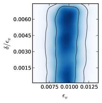
(a) $\;\;\;n=1$

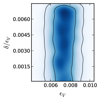
(b) $\;\;\;n=\frac{2}{3}$

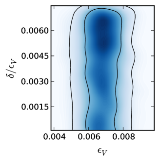
(c) $\;\;\;n=\frac{3}{5}$

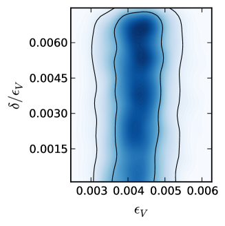
(d) $\;\;\;n=\frac{1}{3}$

Figure 1: Two-dimensional marginalized distribution for the parameters $\delta/\epsilon_{V}$ and $\epsilon_{V}$ at the pivot $k_{0}=0.05\text{Mpc}^{-1}$ for the power-law potential with $n=1$, $n=\frac{2}{3}$, $n=\frac{3}{5}$, and $n=\frac{1}{3}$, respectively. The internal and external lines correspond to the confidence levels of $68\%$ and $95\%$, respectively.

In the following, we run the Cosmological Monte Carlo (CosmoMC) code COSMOMC with the Planck Planck2013 , BAO BAO2013 , and Supernova Legacy Survey SN data for the power-law potential (5.9) for $n=1,\;\frac{3}{5},\;\frac{2}{3},\;\frac{1}{3}$, respectively. It is worthwhile to mention that all these potentials can be naturally realized in the axion monodromy inflation motivated by string/M theory axion . In Zhu3 , by using CosmoMC code COSMOMC , we already extracted constraints on loop quantum correction parameter $\delta_{\text{Pl}}/\epsilon_{V}$ and slow-roll parameter $\epsilon_{V}$ for $\sigma=1$ and $\sigma=2$ when $n=1$. It was noted that the constraint for $\sigma=2$ is much more tighter than the case of $\sigma=1$, and makes the quantum gravitational effects undetectable for models with $\sigma\geq 2$. It is interesting to note that models with small $\sigma$ are also favorable theoretically Bojowald2011 ; Bojowald2011b . Therefore, in the following we shall focus on the observational constraints for the case $\sigma=1$.

We assume the flat cold dark matter model with effective number of neutrinos $N_{eff}=3.046$ and fix the total neutrino mass $\Sigma m_{\nu}=0.06eV$. We vary the seven parameters: (i) baryon density parameter, $\Omega_{b}h^{2}$, (ii) dark matter density parameter, $\Omega_{c}h^{2}$, (iii) the ratio of the sound horiozn to the angular diameter, $\theta$, (iv) the reionization optical depth $\tau$, (v) $\delta(k_{0})/\epsilon_{V}$, (vi) $\epsilon_{V}$, (vii) $\Delta_{s}^{2}(k_{0})$. We take the pivot wave number $k_{0}=0.05\;{\mbox{Mpc}}^{-1}$ used in Planck to constrain $\delta(k_{0})$ and $\epsilon_{V}$. In Fig.1, the constraints on ${\delta}/{\epsilon_{V}}$ and ${\epsilon_{V}}$ are given, respectively, for $n=1$, $n=\frac{2}{3}$, $n=\frac{3}{5}$, and $n=\frac{1}{3}$. In particular, we find that at $68\%$ C.L.,

$$\delta(k_{0})\lesssim 7.9\times 10^{-5},\;\;\;\;\;\text{with}\;\;n=1,$$ (5.17)

$$\delta(k_{0})\lesssim 5.7\times 10^{-5},\;\;\;\;\;\text{with}\;\;n=\frac{2}{3},$$ (5.18)

$$\delta(k_{0})\lesssim 5.4\times 10^{-5},\;\;\;\;\;\text{with}\;\;n=\frac{3}{5},$$ (5.19)

$$\delta(k_{0})\lesssim 3.4\times 10^{-5},\;\;\;\;\;\text{with}\;\;n=\frac{1}{3},$$ (5.20)

which are much tighter than those given in Bojowald2011b . In the above, to get the the bounds on $\delta(k_{0})$, we have used the best-fit values of $\epsilon_{V}$, respectively for different $n$. It is also easy to see that the upper bound for both $\delta(k_{0})$ and $\epsilon_{V}$ decrease slightly as $n$ decreases. However, it is remarkable to note that the up bound on $\delta(k_{0})/\epsilon_{V}$ is rather robust for different values of $n$, which is roughly

$$\frac{\delta(k_{0})}{\epsilon_{V}}\simeq{\cal{O}}(1)\times 10^{-3}\;\;(68\%\;\text{C.L.}).$$ (5.21)

With such bounds, the gravitational quantum effects, denoted by $\mathcal{F}(\sigma)\frac{\delta(k_{0})}{\epsilon_{V}}$ in Eq. (5.15), could be within the range of the detection of the current and forthcoming cosmological experiments S4-CMB . In addition, as we already pointed out in Zhu3 , the up bounds for $\frac{\delta(k_{0})}{\epsilon_{V}}$ increase dramatically as $\sigma$ decreases. Thus it is very promising to expect the detectability of gravitational quantum effects for $\sigma\lesssim 1$ in the forthcoming cosmological experiments.

VI Conclusions

The uniform asymptotic approximation method provides a powerful, systematically improvable, and error-controlled approach to construct accurate analytical solutions of linear perturbations. Its effectiveness has been verified by applying it to the inflation models with nonlinear dispersion relations Uniform3 and $k$-inflation Uniform4 . In this paper, we apply the high-order uniform asymptotic approximation to derive the inflationary observables for scalar and tensor perturbations in LQC with holonomy and inverse-volume quantum corrections. We obtain explicitly the analytical expressions of power spectra, spectral indices, and running of spectral indices up to the third-order approximation in terms of the parameters introduced in the uniform asymptotic approximation method. To this order, the upper error bounds are $\leq 0.15\%$, accurate enough for the current and forthcoming experiments S4-CMB . These expressions are all descibed in terms of the slow-roll parameters (up to the second-order) and the parameters which represent the holonomy and inverse-volume quantum gravitational corrections.

For later applications of our results, we also rewrite all the inflationary observables including power spectra, spectral indices, and running of spectral indices for both scalar and tensor perturbations in terms of quantities evaluated at the time when the inflationary scalar (or tensor mode) crosses the Hubble horizon. With the resulting expressions, the tensor-to-scalar ratio is also obtained, and it is shown that the holonomy corrections do not contribute to the tensor-to-scalar ratio up to the second-order approximations. More interestingly, with the inverse-volume corrections, we find that both scalar and tensor spectra exhibit a deviation from the usual shape at large scales, which could be potentially important for the observational tests. As the uniform asymptotic approximate solution at the third-order has error bounds $\lesssim 0.15\%$, the inflationary observables obtained in the present paper represent the most accurate results obtained so far in the literature.

Utilizing the most accurate CMB, BAO and SN data currently available publicly Planck2013 ; BAO2013 ; SN , we also carry out the CMB likelihood analysis, and find the tightest constraints on $({\delta}(k_{0}),{\epsilon_{V}})$, obtained so far in the literature. Even with such tight constraints, the quantum gravitational effects due to the inverse-volume corrections of LQC can be within the range of the detection of the current and forthcoming cosmological experiments S4-CMB , provided that $\sigma\lesssim 1$.

Appendix A: The uniform asymptotic approximation

In this section, we present a brief introduction of the uniform asymptotic approximation method and its applications to the inflationary cosmology for the cases where the dispersion relation has only a single turning point. For details, we refer readers to our original papers Zhu1 ; Zhu2 ; Uniform3 ; Uniform4 .

A. The approximate solution of the mode function

In the uniform asymptotic approximation method uniformPRL ; Olver1974 ; Zhu1 ; Zhu2 , one usually works with the second-order differential equation,

$$\frac{d^{2}\mu_{k}(y)}{dy^{2}}=\left[\lambda^{2}\hat{g}(y)+q(y)\right]\mu_{k}(y).$$ (A.1)

In the above the parameter $\lambda$ is used to trace the order of the uniform approximations. Usually $\lambda$ is supposed to be large, and it also can be absorbed into $\hat{g}(y)$. Thus when we turn to determine the final results, we can set $\lambda=1$ for the sake of simplicity. For convenience, we also use the notation $g(y)=\lambda^{2}\hat{g}(y)$. Specific to the cosmological applications, $\mu_{k}(y)$ represents the inflationary mode function for cosmological scalar or tensor perturbations, and one can identify

$$\lambda^{2}\hat{g}(y)+q(y)\equiv-\frac{1}{k^{2}}\left(\omega^{2}_{k}(\eta)-\frac{z^{\prime\prime}(\eta)}{z(\eta)}\right),$$ (A.2)

where $\omega_{k}^{2}(\eta)$ is the associated dispersion relation for the inflationary mode function $\mu_{k}(y)$ and $z(\eta)$ depends on the cosmological background evolution. In most of the cases, $\hat{g}(y)$ and $q(y)$ have two poles (singularities): one is at $y=0^{+}$ and the other is at $y=+\infty$. As we discussed in Zhu2 (see also uniformPRL ; Olver1974 ), if these two poles are both second-order or higher, one needs to choose

$$q(y)=-\frac{1}{4y^{2}},$$ (A.3)

for ensuring the convergence of the error control functions. In this paper we shall restrict our investigations to this case. In addition, the function $\hat{g}(y)$ can vanish at various points, which are called turning points or zeros, and the approximate solution of the mode function $\mu_{k}(y)$ depends on the behavior of $\hat{g}(y)$ and $q(y)$ near these turning points.

To proceed further, let us first introduce the Liouville transformation with two new variables $U(\xi)$ and $\xi$ via the relations,

$$U(\xi) = \chi^{1/4}\mu_{k}(y),\;\;\;\xi^{\prime 2}=\frac{|\hat{g}(y)|}{f^{(1)}(\xi)^{2}},$$ (A.4)

where $\chi\equiv\xi^{\prime 2},\;\xi^{\prime}=d\xi/dy$, and

$$f(\xi) = \int^{y}\sqrt{|\hat{g}(y)|}dy,\;\;\;f^{(1)}(\xi)=\frac{df(\xi)}{d\xi}.$$ (A.5)

Note that $\chi$ must be regular and not vanish in the intervals of interest. Consequently, $f(\xi)$ must be chosen so that $f^{(1)}(\xi)$ has zeros and singularities of the same type as that of $\hat{g}(y)$. As shown below, such a requirement plays an essential role in determining the approximate solutions. In terms of $U$ and $\xi$, Eq. (A.1) takes the form

$$\frac{d^{2}U}{d\xi^{2}} = \left[\pm\lambda^{2}f^{(1)}(\xi)^{2}+\psi(\xi)\right]U,$$ (A.6)

where

$$\psi(\xi)=\frac{q(y)}{\chi}-\chi^{-3/4}\frac{d^{2}(\chi^{-1/4})}{dy^{2}},$$ (A.7)

and the signs “$\pm$” correspond to $\hat{g}(y)>0$ and $\hat{g}(y)<0$, respectively. Considering $\psi(\xi)=0$ as the first-order approximation, one can choose $f^{(1)}(\xi)$ so that the first-order approximation can be as close to the exact solution as possible with the guidelines of the error functions constructed below, and then solve it in terms of known functions. Clearly, such a choice sensitively depends on the behavior of the functions $\hat{g}(y)$ and $q(y)$ near the poles and turning points.

In this paper, we consider only the case in which $\hat{g}(y)$ has only one single turning point $\bar{y}_{0}$ (for $\hat{g}(y)$ having several different turning points or one multiple-turning point, see Zhu2 ), i.e., $\hat{g}(\bar{y}_{0})=0$. In this case we can choose

$$f^{(1)}(\xi)^{2}=\pm\xi,$$ (A.8)

where $\xi=\xi(y)$ is a monotone decreasing function, and $\pm$ correspond to $\hat{g}(y)\geq 0$ and $\hat{g}(y)\leq 0$, respectively. Following Olver Olver1974 , the general solution of Eq. (A.6) can be written as

$$U(\xi) = \alpha_{0}\Bigg{[}\text{Ai}(\lambda^{2/3}\xi)\sum_{s=0}^{n}\frac{A_{s}(\xi)}{\lambda^{2s}}$$

$$~{}~{}~{}~{}~{}~{}~{}+\frac{\text{Ai}^{\prime}(\lambda^{2/3}\xi)}{\lambda^{4/3}}\sum_{s=0}^{n-1}\frac{B_{s}(\xi)}{\lambda^{2s}}+\epsilon_{3}^{(2n+1)}\Bigg{]}$$

$$+\beta_{0}\Bigg{[}\text{Bi}(\lambda^{2/3}\xi)\sum_{s=0}^{n}\frac{A_{s}(\xi)}{\lambda^{2s}}$$

$$~{}~{}~{}~{}~{}~{}~{}~{}+\frac{\text{Bi}^{\prime}(\lambda^{2/3}\xi)}{\lambda^{4/3}}\sum_{s=0}^{n-1}\frac{B_{s}(\xi)}{\lambda^{2s}}+\epsilon_{4}^{(2n+1)}\Bigg{]},$$

where $\text{Ai}(x)$ and $\text{Bi}(x)$ represent the Airy functions, $\epsilon_{3}^{(2n+1)}$ and $\epsilon_{4}^{(2n+1)}$ are errors of the approximate solution, and

$$A_{0}(\xi)=1,\;\;$$

$$B_{s}(\xi)=\frac{\pm 1}{2(\pm\xi)^{1/2}}\int_{0}^{\xi}\{\psi(v)A_{s}(v)-A^{\prime\prime}_{s}(v)\}\frac{dv}{(\pm v)^{1/2}},$$

$$A_{s+1}(\xi)=-\frac{1}{2}B^{\prime}_{s}(\xi)+\frac{1}{2}\int\psi(v)B_{s}(v)dv,$$

where $\pm$ correspond to $\xi\geq 0$ and $\xi\leq 0$, respectively. The error bounds of $\epsilon_{3}^{(2n+1)}$ and $\epsilon_{4}^{(2n+1)}$ can be expressed as

$$\frac{\epsilon_{3}^{(2n+1)}}{M(\lambda^{2/3}\xi)},\;\;\frac{\partial\epsilon_{3}^{(2n+1)}/\partial\xi}{\lambda^{2/3}N(\lambda^{2/3}\xi)}$$

$$~{}~{}~{}~{}~{}\leq 2E^{-1}(\lambda^{2/3}\xi)\exp{\left[\frac{2\kappa_{0}\mathscr{V}_{\alpha,\xi}(|\xi^{1/2}|B_{0})}{\lambda}\right]}$$

$$~{}~{}~{}~{}~{}~{}~{}~{}~{}~{}~{}\times\frac{\mathscr{V}_{\alpha,\xi}(|\xi^{1/2}|B_{n})}{\lambda^{2n+1}},$$

$$\frac{\epsilon_{4}^{(2n+1)}}{M(\lambda^{2/3}\xi)},\;\;\frac{\partial\epsilon_{4}^{(2n+1)}/\partial\xi}{\lambda^{2/3}N(\lambda^{2/3}\xi)}$$

$$~{}~{}~{}~{}~{}\leq 2E(\lambda^{2/3}\xi)\exp{\left[\frac{2\kappa_{0}\mathscr{V}_{\xi,\beta}(|\xi^{1/2}|B_{0})}{\lambda}\right]}$$

$$~{}~{}~{}~{}~{}~{}~{}~{}~{}~{}~{}\times\frac{\mathscr{V}_{\xi,\beta}(|\xi^{1/2}|B_{n})}{\lambda^{2n+1}},$$ (A.11)

where the definitions of $M(x)$, $N(x)$, $\kappa_{0}$, and $\mathscr{V}_{a,b}(x)$ can be found in Zhu2 .

B. Power spectra and spectral indices up to the third-order

With the approximate solution given in the last section, now let us begin to calculate the inflationary power spectra and spectral indices from the approximate solution. We assume that the universe was initially at the adiabatic vacuum,

$$\lim_{y\to+\infty}\mu_{k}(y)=\lim_{y\to+\infty}\frac{1}{\sqrt{2\omega_{k}(\eta)}}e^{-i\int\omega_{k}(\eta)d\eta}.$$ (A.12)

Then, we need to match this initial state with the approximate solution (A. The approximate solution of the mode function). However, the approximate solution (A. The approximate solution of the mode function) involves many high-order terms, which are complicated and not easy to handle. In order to simplify them, we first study their behavior in the limit $y\rightarrow+\infty$. Let us start with the $B_{0}(\xi)$ term in Eq. (A. The approximate solution of the mode function), which satisfies

$$B_{0}(\xi)=-\frac{1}{2\sqrt{-\xi}}\int_{0}^{\xi}\frac{\psi(v)}{\sqrt{-v}}dv=-\frac{\mathscr{H}(\xi)}{2\sqrt{-\xi}},$$ (A.13)

where $\mathscr{H}(\xi)\equiv\int_{0}^{\xi}dv\psi(v)/|v|^{1/2}$ is the associated error control function of the approximate solution (A. The approximate solution of the mode function), and in the above we have used $A_{0}(\xi)=1$. The error control function $\mathscr{H}(\xi)$ is well behaved around the turning point $\bar{y}_{0}$ and converges when $y\to+\infty$. As a result, we have

$$\lim_{y\rightarrow+\infty}B_{0}(\xi)=-\frac{\mathscr{H}(-\infty)}{2\sqrt{-\xi}}.$$ (A.14)

Then, let us turn to $A_{1}$, which is

$$A_{1}(\xi)=-\frac{1}{2}B_{0}^{\prime}(\xi)+\frac{1}{2}\int_{0}^{\xi}\psi(v)B_{0}(v)dv.$$ (A.15)

In the limit $y\rightarrow+\infty$, $B_{0}^{\prime}(\xi)$ vanishes, and we find

$$\lim_{y\to+\infty}A_{1}(\xi) = -\frac{1}{2}\int_{0}^{\xi}\frac{\psi(v)}{\sqrt{-v}}\left[\frac{1}{2}\int_{0}^{v}\frac{\psi(u)}{\sqrt{-u}}du\right]dv$$ (A.16)

$$= -\frac{1}{2}\left[\frac{\mathscr{H}(-\infty)}{2}\right]^{2}.$$

Note that in the above we have used the formula

$$n!\int_{\xi_{0}}^{\xi}f(\xi_{n})\int_{\xi_{0}}^{\xi_{n}}f(\xi_{n-1})\cdots\int_{\xi_{0}}^{\xi_{2}}f(\xi_{1})d\xi_{1}d\xi_{2}\cdots d\xi_{n}$$

$$~{}~{}~{}~{}~{}~{}~{}~{}~{}~{}~{}~{}~{}~{}~{}~{}~{}~{}~{}~{}~{}~{}~{}~{}~{}~{}~{}~{}~{}~{}=\left[\int_{\xi_{0}}^{\xi}f(v)dv\right]^{n}.$$ (A.17)

Thus, up to the third-order, we have

$$A_{0}(\xi)+\frac{A_{1}(\xi)}{\lambda^{2}} = 1-\frac{1}{2\lambda^{2}}\left[\frac{\mathscr{H}(-\infty)}{2}\right]^{2}+\mathcal{O}\left(\frac{1}{\lambda^{3}}\right),\;\;\;\;\;$$

$$\frac{B_{0}(\xi)}{\lambda} = -\frac{1}{\sqrt{-\xi}}\frac{\mathscr{H}(-\infty)}{2\lambda}+\mathcal{O}\left(\frac{1}{\lambda^{3}}\right).$$ (A.18)

Using the asymptotic form of Airy functions in the limit $\xi\to-\infty$, and comparing the solution $\mu_{k}(y)$ with the initial state, we obtain

$$\alpha_{0}=\sqrt{\frac{\pi}{2k}}\frac{\lambda^{1/3}}{(A_{0}+A_{1}/\lambda^{2})-i\sqrt{-\xi}B_{0}/\lambda},$$

$$\beta_{0}=i\sqrt{\frac{\pi}{2k}}\frac{\lambda^{1/3}}{(A_{0}+A_{1}/\lambda^{2})-i\sqrt{-\xi}B_{0}/\lambda},$$ (A.19)

where we have

$$(A_{0}+A_{1}/\lambda^{2})-i\sqrt{-\xi}B_{0}/\lambda=(1+\mathcal{O}(1/\lambda^{3}))e^{i\theta}.~{}~{}~{}~{}~{}~{}~{}$$ (A.20)

Here $\theta$ is an irrelevant phase factor, and without loss of generality, we can set $\theta=0$. Thus, we finally get

$$\frac{\alpha_{0}}{\lambda^{1/3}}=\sqrt{\frac{\pi}{2k}},\;\;\;\frac{\beta_{0}}{\lambda^{1/3}}=i\sqrt{\frac{\pi}{2k}}.$$ (A.21)

After determining the coefficients $\alpha_{0}$ and $\beta_{0}$, we can calculate the power spectra of the perturbations. As $y\rightarrow 0$, only the growing mode is relevant. Thus we have

$$\mu_{k}(y) \simeq \beta_{0}\left(\frac{\xi}{\hat{g}(y)}\right)^{1/4}\Bigg{[}\text{Bi}(\lambda^{2/3}\xi)\sum_{s=0}^{+\infty}\frac{B_{s}(\xi)}{\lambda^{2s}}$$ (A.22)

$$\;\;\;\;\;\;\;\;\;\;\;\;+\frac{\lambda^{2/3}\text{Bi}^{\prime}(\lambda^{2/3}\xi)}{\lambda^{2}}\sum_{s=0}^{+\infty}\frac{B_{s}(\xi)}{\lambda^{2s}}\Bigg{]}.\;\;\;\;\;\;\;\;$$

In order to calculate the power spectra to higher order, let us first consider the $B_{0}(\xi)$ term, which satisfies

$$\lim_{y\to 0}B_{0}(\xi)=\frac{1}{2\xi^{1/2}}\int_{0}^{\xi}\frac{\psi(v)}{v^{1/2}}dv=\frac{\mathscr{H}(+\infty)}{2\xi^{1/2}}.$$ (A.23)

In the above we had used the relation $\xi^{1/2}d\xi=-\sqrt{\hat{g}}dy$. Knowing the $B_{0}$ term, we can get the $A_{1}$ term, which is

$$\lim_{y\to 0}A_{1}(\xi) = \frac{1}{4}\int_{0}^{\xi}\frac{\psi(v)}{v^{1/2}}\int_{0}^{v}\frac{\psi(u)}{u^{1/2}}dudv$$ (A.24)

$$= \frac{1}{2}\left[\frac{\mathscr{H}(+\infty)}{2}\right]^{2}.$$

Thus up to the third order and considering the asymptotic forms of the Airy functions in the limit $\xi\rightarrow+\infty$, we find

$$\lim_{y\rightarrow 0}\mu_{k}(y) = \frac{\beta_{0}e^{\frac{2}{3}\lambda\xi^{2/3}}}{\lambda^{1/6}\hat{g}^{1/4}\pi^{1/2}}\Bigg{[}1+\frac{\mathscr{H}(+\infty)}{2\lambda}+\frac{\mathscr{H}(+\infty)^{2}}{8\lambda^{2}}$$ (A.25)

$$~{}~{}~{}~{}~{}~{}~{}~{}~{}~{}~{}~{}~{}~{}~{}~{}~{}~{}~{}~{}~{}~{}~{}~{}+\mathcal{O}(1/\lambda^{3})\Bigg{]}.$$

Then, the power spectra can be calculated, and is given by

$$\Delta^{2}(k) \equiv \frac{k^{3}}{2\pi^{2}}\left|\frac{\mu_{k}(y)}{z}\right|^{2}_{y\to 0^{+}}$$

$$\simeq \frac{k^{2}}{4\pi^{2}}\frac{-k\eta}{z^{2}(\eta)\nu(\eta)}\exp\left(2\int_{y}^{\bar{y}_{0}}\sqrt{{g}(\hat{y})}d\hat{y}\right)$$

$$\;\times\left[1+\frac{\mathscr{H}(+\infty)}{\lambda}+\frac{\mathscr{H}^{2}(+\infty)}{2\lambda^{2}}+\mathcal{O}(1/\lambda^{3})\right].$$

From the power spectra presented above, one can get the general expression of the spectral indices, which now is given by

$$n-1 \equiv \frac{d\ln\Delta^{2}(k)}{d\ln k}$$ (A.27)

$$\simeq 3+2\frac{d}{d\ln k}\int_{y}^{\bar{y}_{0}}\sqrt{g(\hat{y})}d\hat{y}+\frac{1}{\lambda}\frac{d\mathscr{H}(+\infty)}{d\ln k}$$

$$+\mathcal{O}\left(\frac{1}{\lambda^{3}}\right),$$

where the last term in the above expression represents the second- and third-order approximations. It should be noted that the above results represent the most general expressions of the power spectra and spectral indices of perturbations for the case that has only one-turning point.

Appendix B: Integral of $\sqrt{g(y)}$ and the error control function $\mathscr{H}(+\infty)$ with inverse-volume corrections

In general, the integral of $\sqrt{g}$ can be divided into two parts,

$$\int_{y}^{\bar{y}_{0}}\sqrt{g(y)}dy\simeq I_{1}+I_{2},$$ (B.1)

where after some tedious calculations we find

$$\lim_{y\to 0}I_{1} = \bar{y}_{0}\Big{[}-1-\ln\frac{y}{2\bar{y}_{0}}+\left(-\frac{\pi}{2}+\ln 2-\ln\frac{y}{\bar{y}_{0}}\right)A_{0}$$ (B.2)

$$~{}~{}~{}~{}+\frac{1}{2}(-2+\pi)A_{1}+\left(1-\frac{\pi}{4}\right)A_{2}$$

$$~{}~{}~{}~{}+\left(-\frac{2}{3}+\frac{\pi}{4}\right)A_{3}+\left(\frac{2}{3}-\frac{3\pi}{16}\right)A_{4}$$

$$~{}~{}~{}~{}+\left(-\frac{8}{15}+\frac{3\pi}{16}\right)A_{5}+\left(\frac{8}{15}-\frac{5\pi}{32}\right)A_{6}$$

$$~{}~{}~{}~{}+\left(-\frac{16}{35}+\frac{5\pi}{32}\right)A_{7}\Big{]},$$

$$\lim_{y\to 0}I_{2} = \left(-\frac{\pi^{2}}{24}+\frac{\ln^{2}2}{2}-\frac{1}{2}\ln^{2}\frac{y}{\bar{y}_{0}}\right)\bar{y}_{1}$$ (B.3)

$$+\bar{y}_{0}\Bigg{[}\left(-\frac{\pi^{2}}{24}-\ln 2+\frac{\ln^{2}2}{2}-\frac{1}{2}\ln^{2}\frac{y}{\bar{y}_{0}}\right)B_{0}$$

$$-\frac{\pi}{2}B_{1}-B_{2}\ln 2+\left(-\frac{\pi}{2}+\frac{\pi\ln 2}{2}\right)B_{3}$$

$$+(1-\ln 4)B_{4}+\left(-\frac{5\pi}{8}+\frac{3\pi\ln 2}{4}\right)B_{5}$$

$$+\left(\frac{14}{9}-\frac{8\ln 2}{3}\right)B_{6}+\left(\frac{15\pi\ln 2}{16}-\frac{47\pi}{64}\right)B_{7}$$

$$+\left(\frac{148}{75}-\frac{16\ln 2}{5}\right)B_{8}\Bigg{]},$$

where $A_{0},\cdots,A_{7}$, $B_{0},\cdots,B_{8}$, and $C_{0}$ are given by

$$A_{0} = \frac{1}{2}\bar{y}_{0}^{-2+\sigma}\left(-a\bar{m}_{0}+\chi\bar{y}_{0}^{2}\right)\epsilon_{\text{Pl}}\bar{\kappa}_{0},$$

$$A_{1} = \frac{1}{2}\bar{y}_{0}^{-2+\sigma}\left(-b\bar{m}_{0}+\chi\bar{y}_{0}^{2}\right)\epsilon_{\text{Pl}}\bar{\kappa}_{0},$$

$$A_{2} = \frac{1}{2}y_{0}^{-2+\sigma}\left(-c\bar{m}_{0}+a\chi\bar{y}_{0}^{2}\right)\epsilon_{\text{Pl}}\bar{\kappa}_{0},$$

$$A_{3} = \frac{1}{2}\bar{\kappa}_{0}\epsilon_{\text{Pl}}y_{0}^{\sigma-2}\left(b\chi y_{0}^{2}-d\bar{m}_{0}\right),$$

$$A_{4} = \frac{1}{2}\bar{\kappa}_{0}\epsilon_{\text{Pl}}\bar{y}_{0}^{\sigma-2}\left(c\chi\bar{y}_{0}^{2}-e\bar{m}_{0}\right),$$

$$A_{5} = \frac{1}{2}\bar{\kappa}_{0}\epsilon_{\text{Pl}}\bar{y}_{0}^{\sigma-2}\left(d\chi\bar{y}_{0}^{2}-f\bar{m}_{0}\right),$$

$$A_{6} = \frac{1}{2}e\bar{\kappa}_{0}\chi\epsilon_{\text{Pl}}\bar{y}_{0}^{\sigma},$$

$$A_{7} = \frac{1}{2}f\bar{\kappa}_{0}\chi\epsilon_{\text{Pl}}\bar{y}_{0}^{\sigma},$$ (B.4)

and

$$B_{0} = -\frac{a}{2}\epsilon_{\text{Pl}}\bar{y}_{0}^{\sigma-2}\left(\bar{\kappa}_{0}\bar{m}_{1}+\bar{\kappa}_{1}\bar{m}_{0}\right),$$

$$B_{1} = \frac{1}{2}(a-b)\epsilon_{\text{Pl}}\bar{y}_{0}^{\sigma-2}\left(\bar{\kappa}_{0}\bar{m}_{1}+\bar{\kappa}_{1}\bar{m}_{0}\right),$$

$$B_{2} = \frac{1}{2}\epsilon_{\text{Pl}}\bar{y}_{0}^{\sigma-2}(a+b-c)\left(\bar{\kappa}_{0}\bar{m}_{1}+\bar{\kappa}_{1}\bar{m}_{0}\right),$$

$$B_{3} = -\frac{1}{2}\epsilon_{\text{Pl}}\bar{y}_{0}^{\sigma-2}\left(\bar{\kappa}_{0}\bar{m}_{1}+\bar{\kappa}_{1}\bar{m}_{0}\right)(a-b-c+d),$$

$$B_{4} = -\frac{1}{2}\epsilon_{\text{Pl}}\bar{y}_{0}^{\sigma-2}\left(\bar{\kappa}_{0}\bar{m}_{1}+\bar{\kappa}_{1}\bar{m}_{0}\right)(b-c-d+e),$$

$$B_{5} = -\frac{1}{2}\epsilon_{\text{Pl}}\bar{y}_{0}^{\sigma-2}\left(\bar{\kappa}_{0}\bar{m}_{1}+\bar{\kappa}_{1}\bar{m}_{0}\right)(c-d-e+f),$$

$$B_{6} = -\frac{1}{2}\epsilon_{\text{Pl}}\bar{y}_{0}^{\sigma-2}(d-e-f)\left(\bar{\kappa}_{0}\bar{m}_{1}+\bar{\kappa}_{1}\bar{m}_{0}\right),$$

$$B_{7} = -\frac{1}{2}(e-f)\epsilon_{\text{Pl}}\bar{y}_{0}^{\sigma-2}\left(\bar{\kappa}_{0}\bar{m}_{1}+\bar{\kappa}_{1}\bar{m}_{0}\right),$$

$$B_{8} = -\frac{1}{2}f\epsilon_{\text{Pl}}\bar{y}_{0}^{\sigma-2}\left(\bar{\kappa}_{0}\bar{m}_{1}+\bar{\kappa}_{1}\bar{m}_{0}\right).$$ (B.5)

The error control function $\mathscr{H}(+\infty)$ can also be obtained by employing the expansions given in Eq. (3.27), and we find

$$\frac{\mathscr{H}(+\infty)}{\lambda} \simeq \frac{1}{6\bar{y}_{0}}-\frac{(23+12\ln 2)\bar{y}_{1}}{72\bar{y}_{0}^{2}}$$

$$+\Bigg{[}\frac{\pi a}{16}+\left(\frac{2}{3}-\frac{\pi}{16}\right)b+\left(\frac{15\pi}{32}-\frac{2}{3}\right)c$$

$$~{}~{}~{}~{}+\left(\frac{8}{3}-\frac{15\pi}{32}\right)d+\left(\frac{175\pi}{128}-\frac{8}{3}\right)e$$

$$~{}~{}~{}~{}+\left(\frac{32}{5}-\frac{175\pi}{128}\right)f-\frac{1}{12}\Bigg{]}\chi\epsilon_{\text{Pl}}\bar{y}_{0}^{\sigma-1}\bar{\kappa}_{0}$$

$$+\Bigg{(}\frac{a}{12}-\frac{2d}{3}+\frac{2e}{3}-\frac{8f}{3}-\frac{c\pi}{16}+\frac{d\pi}{16}$$

$$~{}~{}~{}~{}-\frac{15e\pi}{32}+\frac{15f\pi}{32}\Bigg{)}\bar{m}_{0}\epsilon_{\text{Pl}}\bar{\kappa}_{0}\bar{y}_{0}^{\sigma-3}$$

$$+\Bigg{[}\left(\frac{23}{144}+\frac{\pi}{48}+\frac{\ln 2}{12}\right)a-\left(\frac{1}{12}+\frac{\pi}{48}\right)b$$

$$~{}~{}~{}~{}+\left(\frac{1}{12}-\frac{7\pi}{48}+\frac{\pi\ln 2}{16}\right)c$$

$$~{}~{}~{}~{}+\left(\frac{7\pi}{48}-\frac{1}{6}-\frac{2\ln 2}{3}-\frac{\pi\ln 2}{16}\right)d$$

$$~{}~{}~{}~{}+\left(\frac{1}{6}-\frac{41\pi}{64}+\frac{2\ln 2}{3}+\frac{15\pi\ln 2}{32}\right)e$$

$$~{}~{}~{}~{}+\left(\frac{4}{9}+\frac{41\pi}{64}-\frac{8\ln 2}{3}-\frac{15\pi\ln 2}{32}\right)f\Bigg{]}$$

$$~{}~{}~{}~{}~{}~{}~{}~{}~{}~{}\times\left(\bar{\kappa}_{0}\bar{m}_{1}+\bar{\kappa}_{1}\bar{m}_{0}\right)\epsilon_{\text{Pl}}\bar{y}_{0}^{\sigma-3}.$$

Once we get the integral of $\sqrt{g(y)}$ in Eq. (B.2) and the error control function in Eq. (Appendix B: Integral of $\sqrt{g(y)}$ and the error control function $\mathscr{H}(+\infty)$ with inverse-volume corrections), from Eq. (B. Power spectra and spectral indices up to the third-order) we can easily calculate the power spectra.

Now we turn to consider the corresponding spectral indices. In order to do this, we first specify the $k$-dependence of $\bar{y}_{0}(\eta_{0})$, $\bar{y}_{1}(\eta_{0})$, $\bar{\epsilon}_{\text{Pl}}(\eta_{0})$, and $\bar{m}(\eta_{0})$ through $\eta_{0}=\eta_{0}(k)$. From $g(y_{0})=0$ we find

$$\bar{y}_{0}\simeq\bar{\nu}_{0}+\frac{1}{2}\epsilon_{\text{Pl}}\big{(}\bar{m}_{0}\bar{\nu}_{0}^{\sigma-1}-\chi\bar{\nu}_{0}^{\sigma+1}\big{)}\bar{\kappa}_{0},$$ (B.7)

and noticing $-k\eta_{0}=\bar{y}_{0}(\eta_{0})$ and $\epsilon_{\text{Pl}}\sim k^{-\sigma}$, we obtain

$$\frac{d\ln(-\eta_{0})}{d\ln k} \simeq -\left(1+\frac{\bar{y}_{1}}{\bar{y}_{0}}\right)\left[1+\frac{\sigma}{2}\epsilon_{\text{Pl}}\big{(}\bar{m}_{0}\bar{\nu}_{0}^{\sigma-2}-\chi\bar{\nu}_{0}^{\sigma}\big{)}\bar{\kappa}_{0}\right].$$

Then, using the above relation, the spectral indices are given by

$$n-1 \simeq 3-2\bar{\nu}_{0}+\left(\frac{1}{6\bar{\nu}_{0}^{2}}-\ln 4\right)\bar{\nu}_{1}$$ (B.9)

$$+\epsilon_{\text{Pl}}\left(\bar{m}_{1}\bar{\kappa}_{0}+\bar{m}_{0}\bar{\kappa}_{1}\right)\left(\Sigma_{1}\bar{\nu}_{0}^{\sigma-3}+\Sigma_{2}\bar{\nu}_{0}^{\sigma-1}\right)$$

$$+\epsilon_{\text{Pl}}\chi\bar{\kappa}_{0}\left(\Sigma_{3}\bar{\nu}_{0}^{\sigma-1}+\Sigma_{4}\bar{\nu}_{0}^{\sigma+1}\right)$$

$$+\epsilon_{\text{Pl}}\chi\bar{\kappa}_{1}\left(\Sigma_{5}\bar{\nu}_{0}^{\sigma-1}+\Sigma_{6}\bar{\nu}_{0}^{\sigma+1}\right)$$

$$+\epsilon_{\text{Pl}}\bar{m}_{0}\bar{\kappa}_{0}\left(\Sigma_{7}\bar{\nu}_{0}^{\sigma-3}+\Sigma_{8}\bar{\nu}_{0}^{\sigma-1}\right),$$

where $\Sigma_{i},\;i=1,\cdots 8$ depend on the value of $\sigma$ and are given in the Table I. Then the corresponding spectral index reads

$$\alpha \simeq 2\bar{\nu}_{1}-\sigma\epsilon_{\text{Pl}}\bar{m}_{0}\bar{\kappa}_{0}\left(\bar{\nu}_{0}^{\sigma-3}\Sigma_{7}+\bar{\nu}_{0}^{\sigma-1}\Sigma_{8}\right)$$ (B.10)

$$-\epsilon_{\text{Pl}}(m_{1}\bar{\kappa}_{0}+\bar{m}_{0}\bar{\kappa}_{1})[\bar{\nu}_{0}^{\sigma-3}\left(\sigma\Sigma_{1}+\Sigma_{7}\right)$$

$$~{}~{}~{}~{}~{}~{}~{}~{}~{}~{}~{}~{}~{}~{}~{}~{}~{}~{}~{}~{}~{}~{}~{}~{}~{}~{}~{}~{}+\bar{\nu}_{0}^{\sigma-1}\left(\sigma\Sigma_{2}+\Sigma_{8}\right)\Big{]}$$

$$-\sigma\chi\epsilon_{\text{Pl}}\bar{\kappa}_{0}\left(\bar{\nu}_{0}^{\sigma-1}\Sigma_{3}+\bar{\nu}_{0}^{\sigma+1}\Sigma_{4}\right).$$

Appendix C: Slow-roll expansions of $\nu(\eta)$, $c_{s}(\eta)$, $m(\eta)$, $\kappa(\eta)$, and their derivatives

VI.1 Expansions with the holonomy corrections

Let us first consider the scalar perturbation with the holonomy corrections. Using the expression of $z^{\prime\prime}/z$ in Eq. (II.2), it is easy to find that $\nu(\eta)$ for scalar perturbations reads

$$\nu^{s}(\eta) \simeq \frac{3}{2}+\epsilon_{1}+\frac{\epsilon_{2}}{2}+\epsilon_{1}^{2}+\frac{11\epsilon_{2}\epsilon_{1}}{6}+\frac{\epsilon_{2}\epsilon_{3}}{6}-2\epsilon_{1}\delta_{H}$$ (C.1)

$$-\frac{2\epsilon_{1}^{2}\delta_{H}}{3}-6\epsilon_{1}\delta_{H}^{2}-\frac{2\epsilon_{2}\epsilon_{1}\delta_{H}}{3}+\epsilon_{1}^{3}+\frac{77}{18}\epsilon_{2}\epsilon_{1}^{2}$$

$$+\frac{17}{9}\epsilon_{2}^{2}\epsilon_{1}+\frac{14}{9}\epsilon_{2}\epsilon_{3}\epsilon_{1}-\frac{\epsilon_{2}^{2}\epsilon_{3}}{18}.$$

Consideration of the derivatives of $\nu^{s}(\eta)$ with respect to $\ln{(-\eta)}$ yields

$$\nu_{1}^{s} \simeq -\epsilon_{1}\epsilon_{2}-\frac{\epsilon_{3}\epsilon_{2}}{2}-4\epsilon_{1}^{2}\delta_{H}+2\epsilon_{2}\epsilon_{1}\delta_{H}-3\epsilon_{2}\epsilon_{1}^{2}$$ (C.2)

$$-\frac{11}{6}\epsilon_{2}^{2}\epsilon_{1}-\frac{7\epsilon_{2}\epsilon_{3}}{3}\epsilon_{1}-\frac{\epsilon_{2}\epsilon_{3}^{2}}{6}-\frac{\epsilon_{2}\epsilon_{3}\epsilon_{4}}{6}$$

$$-\frac{16}{3}\epsilon_{1}^{3}\delta_{H}-28\epsilon_{1}^{2}\delta_{H}^{2}+2\epsilon_{2}\epsilon_{1}^{2}\delta_{H}+\frac{2}{3}\epsilon_{2}^{2}\epsilon_{1}\delta_{H}$$

$$+6\epsilon_{2}\epsilon_{1}\delta_{H}^{2}+\frac{2}{3}\epsilon_{2}\epsilon_{3}\epsilon_{1}\delta_{H}-6\epsilon_{2}\epsilon_{1}^{3}-\frac{205}{18}\epsilon_{2}^{2}\epsilon_{1}^{2}$$

$$-\frac{119}{18}\epsilon_{2}\epsilon_{3}\epsilon_{1}^{2}-\frac{17}{9}\epsilon_{2}^{3}\epsilon_{1}-\frac{31}{18}\epsilon_{2}\epsilon_{3}^{2}\epsilon_{1}-\frac{35}{6}\epsilon_{2}^{2}\epsilon_{3}\epsilon_{1}$$

$$-\frac{31}{18}\epsilon_{2}\epsilon_{3}\epsilon_{4}\epsilon_{1}+\frac{\epsilon_{2}^{2}\epsilon_{3}^{2}}{9}+\frac{\epsilon_{2}^{2}\epsilon_{3}\epsilon_{4}}{18},$$

$$\nu_{2}^{s} \simeq \epsilon_{1}\epsilon_{2}^{2}+\frac{\epsilon_{3}^{2}\epsilon_{2}}{2}+\epsilon_{1}\epsilon_{3}\epsilon_{2}+\frac{\epsilon_{3}\epsilon_{4}\epsilon_{2}}{2}-8\epsilon_{1}^{3}\delta_{H}$$ (C.3)

$$+12\epsilon_{2}\epsilon_{1}^{2}\delta_{H}-2\epsilon_{2}^{2}\epsilon_{1}\delta_{H}-2\epsilon_{2}\epsilon_{3}\epsilon_{1}\delta_{H}+7\epsilon_{2}^{2}\epsilon_{1}^{2}$$

$$+4\epsilon_{2}\epsilon_{3}\epsilon_{1}^{2}+\frac{11}{6}\epsilon_{2}^{3}\epsilon_{1}+\frac{17}{6}\epsilon_{2}\epsilon_{3}^{2}\epsilon_{1}+6\epsilon_{2}^{2}\epsilon_{3}\epsilon_{1}$$

$$+\frac{17}{6}\epsilon_{2}\epsilon_{3}\epsilon_{4}\epsilon_{1}+\frac{\epsilon_{2}\epsilon_{3}^{3}}{6}+\frac{\epsilon_{2}\epsilon_{3}\epsilon_{4}^{2}}{6}+\frac{\epsilon_{2}\epsilon_{3}^{2}\epsilon_{4}}{2}$$

$$+\frac{\epsilon_{2}\epsilon_{3}\epsilon_{4}\epsilon_{5}}{6},$$

and

$$\nu_{3}^{s} \simeq -\epsilon_{1}\epsilon_{2}^{3}-3\epsilon_{1}\epsilon_{3}\epsilon_{2}^{2}-\frac{\epsilon_{3}^{3}\epsilon_{2}}{2}-\epsilon_{1}\epsilon_{3}^{2}\epsilon_{2}-\frac{\epsilon_{3}\epsilon_{4}^{2}\epsilon_{2}}{2}$$ (C.4)

$$-\frac{3}{2}\epsilon_{3}^{2}\epsilon_{4}\epsilon_{2}-\epsilon_{1}\epsilon_{3}\epsilon_{4}\epsilon_{2}-\frac{1}{2}\epsilon_{3}\epsilon_{4}\epsilon_{5}\epsilon_{2}.$$

For the tensor perturbations, using Eq. (II.2), we find

$$\nu^{t}(\eta) \simeq \frac{3}{2}+\epsilon_{1}+\epsilon_{1}^{2}+\frac{4\epsilon_{1}\epsilon_{2}}{3}-2\delta_{H}\epsilon_{1}-6\delta_{H}^{2}\epsilon_{1}+\epsilon_{1}^{3}$$

$$-\frac{2}{3}\delta_{H}\epsilon_{1}^{2}-\frac{2}{3}\delta_{H}\epsilon_{1}\epsilon_{2}+\frac{34}{9}\epsilon_{1}^{2}\epsilon_{2}+\frac{4}{3}\epsilon_{1}\epsilon_{2}^{2}+\frac{4}{3}\epsilon_{1}\epsilon_{2}\epsilon_{3},$$

$$\nu_{1}^{t} \simeq -\epsilon_{1}\epsilon_{2}-4\delta_{H}\epsilon_{1}^{2}+2\delta_{H}\epsilon_{1}\epsilon_{2}-3\epsilon_{1}^{2}\epsilon_{2}-\frac{4}{3}\epsilon_{1}\epsilon_{2}^{2}$$ (C.6)

$$-\frac{4}{3}\epsilon_{1}\epsilon_{2}\epsilon_{3}+28\delta_{H}^{2}\epsilon_{1}^{2}+\frac{16}{3}\delta_{H}\epsilon_{1}^{3}-6\delta_{H}^{2}\epsilon_{1}\epsilon_{2}$$

$$-2\delta_{H}\epsilon_{1}^{2}\epsilon_{2}+6\epsilon_{1}^{3}\epsilon_{2}-\frac{2}{3}\delta_{H}\epsilon_{1}\epsilon_{2}^{2}+\frac{89}{9}\epsilon_{1}^{2}\epsilon_{2}^{2}$$

$$+\frac{4}{3}\epsilon_{1}\epsilon_{2}^{3}-\frac{2}{3}\delta_{H}\epsilon_{1}\epsilon_{2}\epsilon_{3}+\frac{46}{9}\epsilon_{1}^{2}\epsilon_{2}\epsilon_{3}+4\epsilon_{1}\epsilon_{2}^{2}\epsilon_{3}$$

$$+\frac{4}{3}\epsilon_{1}\epsilon_{2}\epsilon_{3}^{2}+\frac{4}{3}\epsilon_{1}\epsilon_{2}\epsilon_{3}\epsilon_{4},$$

$$\nu_{2}^{t} \simeq \epsilon_{1}\epsilon_{2}^{2}+\epsilon_{1}\epsilon_{2}\epsilon_{3}-8\delta_{H}\epsilon_{1}^{3}+12\delta_{H}\epsilon_{1}^{2}\epsilon_{2}-2\delta_{H}\epsilon_{1}\epsilon_{2}^{2}$$ (C.7)

$$+7\epsilon_{1}^{2}\epsilon_{2}^{2}+\frac{4}{3}\epsilon_{1}\epsilon_{2}^{3}-2\delta_{H}\epsilon_{1}\epsilon_{2}\epsilon_{3}+4\epsilon_{1}^{2}\epsilon_{2}\epsilon_{3}$$

$$+4\epsilon_{1}\epsilon_{2}^{2}\epsilon_{3}+\frac{4}{3}\epsilon_{1}\epsilon_{2}\epsilon_{3}^{2}+\frac{4}{3}\epsilon_{1}\epsilon_{2}\epsilon_{3}\epsilon_{4},$$

and

$$\nu_{3}^{t} \simeq -\epsilon_{1}\epsilon_{2}^{3}-3\epsilon_{1}\epsilon_{3}\epsilon_{2}^{2}-\epsilon_{1}\epsilon_{3}^{2}\epsilon_{2}-\epsilon_{1}\epsilon_{3}\epsilon_{4}\epsilon_{2}.$$

Now we turn to consider $c_{s}(\eta)$. Expanding it in terms of $\delta_{H}$, we observe that

$$c_{s}(\eta) \equiv \sqrt{1-2\delta_{H}}\simeq 1-\delta_{H}-\frac{\delta_{H}^{3}}{2}-\frac{\delta_{H}^{2}}{2}.$$ (C.9)

Similar to $\nu^{s}(\eta)$, the derivatives of $c_{s}(\eta)$ with respect to $\ln{(-\eta)}$ are given by

$$c_{1}(\eta) \simeq -2\epsilon_{1}\delta_{H}-2\epsilon_{1}^{2}\delta_{H}-4\epsilon_{1}\delta_{H}^{2}-9\epsilon_{1}\delta_{H}^{3}-4\epsilon_{1}^{2}\delta_{H}^{2}$$ (C.10)

$$-2\epsilon_{1}^{2}\epsilon_{2}\delta_{H}-2\epsilon_{1}^{3}\delta_{H},$$

$$c_{2}(\eta) \simeq -4\epsilon_{1}^{2}\delta_{H}+2\epsilon_{2}\epsilon_{1}\delta_{H}-8\epsilon_{1}^{3}\delta_{H}-20\epsilon_{1}^{2}\delta_{H}^{2}$$ (C.11)

$$+6\epsilon_{2}\epsilon_{1}^{2}\delta_{H}+4\epsilon_{2}\epsilon_{1}\delta_{H}^{2},$$

and

$$c_{3}(\eta) \simeq -8\epsilon_{1}^{3}\delta_{H}+12\epsilon_{2}\epsilon_{1}^{2}\delta_{H}-2\epsilon_{2}^{2}\epsilon_{1}\delta_{H}-2\epsilon_{2}\epsilon_{3}\epsilon_{1}\delta_{H}.$$

Note that for both scalar and tensor perturbations, the effective sound speed $c_{s}(\eta)$ takes the same form. Thus in the following, we are not going to distinguish them.

VI.2 Expansions with inverse-volume corrections

Now let us turn to consider the slow-roll expansions of $\nu$, $m(\eta)$ and $\kappa(\eta)$. For $\nu(\eta)$ and its derivatives, it is worth to note that when one considers the inverse-volume corrections, $\nu(\eta)$ and its derivatives with respect to $\ln(-\eta)$, i.e., $\nu_{0},\;\nu_{1},\;\nu_{2},\;\text{and}\;\nu_{3}$ all take the same form as those given in general relativity. Thus, they can be directly obtained from Eqs. (C.1)-(C.4) for the scalar perturbations and from Eqs. (VI.1)-(VI.1) for the tensor perturbations by taking the holonomy parameter $\delta_{H}=0$. For the scalar perturbations, on the other hand, the function $m(\eta)$ reads

$$m^{s}(\eta) = \frac{\sigma^{2}\left(3-\sigma\right)\alpha_{0}}{4\epsilon_{1}}$$ (C.13)

$$+\left(\frac{3\sigma}{2}-\frac{\sigma^{2}}{4}-\frac{\sigma^{3}}{12}\right)\vartheta_{0}+\left(\frac{5\sigma^{2}}{4}-\frac{\sigma^{3}}{2}\right)\alpha_{0}$$

$$+\frac{\sigma\alpha_{0}(\sigma-3)\epsilon_{2}}{4\epsilon_{1}}+\frac{\sigma\alpha_{0}\epsilon_{2}\epsilon_{3}}{4\epsilon_{1}}.$$

Note that at the turning point we write $m(\eta_{0})=\bar{m}_{0}$. Now consideration of the derivatives of $m(\eta)$ with respect to $\ln(-\eta)$ yields

$$m_{1}^{s} = \frac{\sigma^{2}\alpha_{0}(3-\sigma)\epsilon_{2}}{4\epsilon_{1}}.$$ (C.14)

Similarly, for tensor perturbations, we have

$$m^{t}(\eta) \simeq \frac{3\sigma\alpha_{0}}{2}-\frac{\sigma^{2}\alpha_{0}}{2},$$ (C.15)

while up to the second-order in the slow-roll parameters we have $m_{2}^{t}\simeq 0$ and $m_{3}^{t}\simeq 0$. Note that we also write $m^{t}(\eta_{0})$ as $\bar{m}_{0}$.

To get the slow-roll expansions of the inflationary observables, we also need the slow-roll expansions of $\kappa(\eta)$ and its derivatives, which are given by

$$\kappa(\eta) = H^{\sigma}\Big{(}1-\sigma\epsilon_{1}\Big{)},$$ (C.16)

$$\kappa_{1} = \sigma H^{\sigma}\epsilon_{1}.$$

Note that at the turning point we write $\kappa(\eta_{0})=\bar{\kappa}_{0}$.

Table 1: Values of Coefficients $\Sigma_{i}(i=1,\dots,8)$ for different values of $\sigma$.

$\sigma$	1	2	3	4	5	6
$\Sigma_{1}$	$-\frac{\pi}{48}$	$\frac{1}{6}$	$\frac{(8-3\ln 2)\pi}{16}$	$\frac{4+8\ln 2}{3}$	$\frac{5(47-30\ln 2)\pi}{64}$	$16\ln 2$
$\Sigma_{2}$	$\frac{(\ln 2-1)\pi}{2}$	$1-2\ln 2$	$\frac{(6\ln 2-5)\pi}{8}$	$\frac{14-24\ln 2}{9}$	$\frac{(60\ln 2-47)\pi}{64}$	$\frac{4(37-60\ln 2)}{75}$
$\Sigma_{3}$	$-\frac{\pi}{16}$	$-\frac{4}{3}$	$-\frac{45\pi}{32}$	$-\frac{32}{3}$	$-\frac{875\pi}{128}$	$-\frac{192}{5}$
$\Sigma_{4}$	$\frac{\pi}{4}$	$\frac{4}{3}$	$\frac{9\pi}{16}$	$\frac{32}{15}$	$\frac{25\pi}{32}$	$\frac{96}{35}$
$\Sigma_{5}$	$-\frac{\pi}{16}-\frac{23}{144}-\frac{\ln 2}{12}$	$-\frac{71}{72}-\frac{\ln 2}{6}$	$-\frac{15\pi}{32}-\frac{23}{48}-\frac{\ln 2}{4}$	$-\frac{119}{36}-\frac{\ln 2}{3}$	$-\frac{175\pi}{128}-\frac{115}{144}-\frac{5\ln 2}{12}$	$-\frac{883}{120}-\frac{\ln 2}{2}$
$\Sigma_{6}$	$-\frac{\pi}{16}-\frac{23}{144}-\frac{\ln 2}{12}$	$-\frac{71}{72}-\frac{\ln 2}{6}$	$-\frac{15\pi}{32}-\frac{23}{48}-\frac{\ln 2}{4}$	$-\frac{119}{36}-\frac{\ln 2}{3}$	$-\frac{175\pi}{128}-\frac{115}{144}-\frac{5\ln 2}{12}$	$-\frac{883}{120}-\frac{\ln 2}{2}$
$\Sigma_{7}$	$0$	$0$	$\frac{3\pi}{16}$	$\frac{8}{3}$	$\frac{75\pi}{32}$	$16$
$\Sigma_{8}$	$-\frac{\pi}{2}$	$-2$	$-\frac{3\pi}{4}$	$-\frac{8}{3}$	$-\frac{15\pi}{16}$	$-\frac{16}{5}$

Table 2: Values of Coefficients $\mathcal{\bar{Q}}_{i}^{(s,t)}$, $\mathcal{\bar{K}}_{i}^{(s,t)}$, $\mathcal{\bar{L}}_{i}^{(s,t)}(i=-1,0,1)$ for different values of $\sigma$.

$\sigma$	1	2	3	4	5	6
$\frac{\mathcal{\bar{Q}}_{-1}^{(s)}}{\alpha_{0}}$	$\frac{\pi}{6}$	$\frac{2}{3}$	$0$	$-\frac{1616}{1629}$	$\frac{475\pi}{2896}$	$\frac{10512}{905}$
$\frac{\mathcal{\bar{Q}}_{0}^{(s)}}{\alpha_{0}}$	$-\frac{2}{9}-\frac{45401\pi}{52128}+\frac{\pi\ln 2}{6}$	$\frac{8\ln 2}{3}-\frac{14647}{3258}$	$\frac{513\pi}{11584}$	$\frac{82702}{8145}-\frac{3232\ln 2}{543}$	$\frac{50}{9}+\frac{743995\pi}{139008}-\frac{1425\pi\ln 2}{2896}$	$\frac{84096\ln 2}{905}-\frac{715864}{31675}$
$\frac{\mathcal{\bar{Q}}_{1}^{(s)}}{\alpha_{0}}$	$\frac{176\pi}{1629}-\frac{1}{9}$	$\frac{4\ln 2}{3}-\frac{985}{1629}$	$0$	$\frac{5732}{4887}-\frac{3232\ln 2}{1629}$	$\frac{25}{9}+\frac{17165\pi}{34752}$	$\frac{58418}{4525}+\frac{21024\ln 2}{905}$
$\frac{\mathcal{\bar{K}}_{-1}^{(s)}}{\alpha_{0}}$	$-\frac{\pi}{6}$	$-\frac{4}{3}$	$0$	$\frac{320}{81}$	$-\frac{125\pi}{144}$	$-\frac{352}{5}$
$\frac{\mathcal{\bar{K}}_{0}^{(s)}}{\alpha_{0}}$	$\frac{20\pi}{81}+\frac{\pi\ln 2}{6}$	$\frac{251}{81}-\frac{8\ln 2}{3}$	$-\frac{9\pi}{64}$	$\frac{1280\ln 2}{81}-\frac{22696}{1215}$	$\frac{625\pi\ln 2}{144}-\frac{104075\pi}{3456}$	$-\frac{26888}{525}-\frac{2112\ln 2}{5}$
$\frac{\mathcal{\bar{K}}_{1}^{(s)}}{\alpha_{0}}$	$\frac{\pi\ln 2}{6}-\frac{109\pi}{324}$	$-\frac{32}{81}-\frac{4\ln 2}{3}$	$0$	$\frac{320}{243}+\frac{320\ln 2}{81}$	$\frac{125\pi\ln 2}{144}-\frac{5225\pi}{1728}$	$-\frac{5944}{75}-\frac{352\ln 2}{5}$
$\frac{\mathcal{\bar{K}}_{2}^{(s)}}{\alpha_{0}}$	$\frac{10165\pi}{15552}-\frac{\pi\ln 2}{12}$	$\frac{524}{243}-2\ln 2$	$\frac{27\pi\ln 2}{64}-\frac{197\pi}{256}$	$\frac{58976\ln 2}{1215}-\frac{101072}{2025}$	$-\frac{13175\pi}{2592}-\frac{95875\pi\ln 2}{3456}$	$\frac{4432\ln 2}{35}-\frac{913732}{3675}$
$\frac{\mathcal{L}^{(s)}_{-1}}{\alpha_{0}}$	$\frac{\pi}{6}$	$\frac{8}{3}$	$0$	$-\frac{1280}{81}$	$\frac{625\pi}{144}$	$\frac{2112}{5}$
$\frac{\mathcal{L}^{(s)}_{0}}{\alpha_{0}}$	$-\frac{13\pi}{162}-\frac{\pi\ln 2}{6}$	$\frac{16\ln 2}{3}-\frac{286}{81}$	$\frac{27\pi}{64}$	$\frac{71584}{1215}-\frac{5120\ln 2}{81}$	$\frac{535375\pi}{3456}-\frac{3125\pi\ln 2}{144}$	$\frac{127696}{175}+\frac{12672\ln 2}{5}$
$\frac{\mathcal{L}^{(s)}_{1}}{\alpha_{0}}$	$\frac{163\pi}{324}-\frac{\pi\ln 2}{6}$	$\frac{172}{81}+\frac{8\ln 2}{3}$	$0$	$-\frac{2240}{243}-\frac{1280\ln 2}{81}$	$\frac{27625\pi}{1728}-\frac{625\pi\ln 2}{144}$	$\frac{13648}{25}+\frac{2112\ln 2}{5}$
$\frac{\mathcal{\bar{Q}}_{0}^{(t)}}{\alpha_{0}}$	$-\frac{725\pi}{2172}$	$-\frac{244}{543}$	$0$	$\frac{11728}{8145}$	$\frac{8165\pi}{5792}$	$\frac{13920}{1267}$
$\frac{\mathcal{\bar{K}}_{0}^{(t)}}{\alpha_{0}}$	$\frac{\pi}{3}$	$\frac{8}{9}$	$0$	$-\frac{2368}{405}$	$-\frac{1025\pi}{144}$	$-\frac{6976}{105}$
$\frac{\mathcal{\bar{L}}_{0}^{(t)}}{\alpha_{0}}$	$-\frac{\pi}{3}$	$-\frac{16}{9}$	$0$	$\frac{9472}{405}$	$\frac{5125\pi}{144}$	$\frac{13952}{35}$

References

- (1) A. Guth, Phys. Rev. D23, 347 (1981); A.A. Starobinsky, Phys. Lett. B 91, 99 (1980); K. Sato, Mon. Not. R. Astron. Soc. 195, 467 (1981).
- (2) D. Baumann, arXiv:0907.5424.
- (3) E. Komatsu et al. (WMAP Collaboration), Astrophys. J. Suppl. Ser. 192, 18 (2011); D. Larson et al. (WMAP Collaboration), ibid., 192, 16 (2011).
- (4) P. Ade et al. (PLANCK Collaboration), arXiv:1303.5082.
- (5) P.A.R. Ade et al. (BICEP2 Collaboration), Phys. Rev. Lett.112, 241101 (2014).
- (6) P.A.R. Ade, et al. (BICEP2/Keck and Planck Collaborations), arXiv:1502.00612; R. Adam, et al. (Planck Collaborations), arXiv:1502.01582.
- (7) M.J. Mortonson and U. Seljak, J. Cosmol. Astropart. Phys.10 (2014) 035; R. Flauger, J.C. Hill and D.N. Spergel, J. Cosmol. Astropart. Phys. 1408 (2014) 039.
- (8) C.P. Burgess, M. Cicoli, and F. Quevedo, JCAP 11 (2013) 003; R.H. Brandenberger and J. Martin, Class. Quantum. Grav. 30 (2013) 113001.
- (9) M. Bojowald, Phys. Rev. Lett. 86, 5227 (2001).
- (10) A. Ashtekar, T. Pawlowski, and P. Singh, Phys. Rev. Lett. 96, 141301 (2006); Phys. Rev. D73, 124038 (2006); Phys. Rev. D74, 084003 (2006); A. Ashtekar, A. Corichi, and P. Singh, Phys. Rev. D77, 024046 (2008).
- (11) M. Bojowald, Rep. Prog. Phys. 78 (2015) 023901; A. Ashtekar and A. Barrau, arXiv:1504.07559.
- (12) J. Mielczarek, J. Cosmol. Astropart. Phys. 11 (2008) 011; Phys. Rev. D79, 123520 (2009); J. Mielczarek, T. Cailleteau, J. Grain, and A. Barrau, Phys. Rev. D81, 104049 (2010).
- (13) J. Grain and A. Barrau, Phys. Rev. Lett. 102, 081301 (2009).
- (14) J. Grain, A. Barrau, T. Cailleteau, and J. Mielczarek, Phys. Rev. D82, 123520 (2010).
- (15) Y. Li and J.-Y Zhu, Class. Quantum Grav. 28, 045007 (2011); J. Mielczarek, T. Cailleteau, A. Barrau and J. Grain, Class. Quantum Grav. 29, 085009 (2012).
- (16) T. Cailleteau, J. Mielczarek, A. Barrau and J. Grain, Class. Quantum Grav. 29, 095010 (2012).
- (17) T. Cailleteau, A. Barrau, F. Vidotto, and J, Grain, Phys. Rev. D86, 087301 (2012).
- (18) A. Barrau, T. Cailleteau, J. Grain, and J. Mielczarek, arXiv: 1309.6896.
- (19) M. Bojowald and G.M. Hossain, Phys. Rev. D78, 063547 (2008).
- (20) M. Bojowald, G.M. Hossain, M. Kagan, and S. Shankaranarayanan, Phys. Rev. D79, 043505 (2009); D82, 109903 (E) (2010).
- (21) M. Bojowald and G.M. Hossain, Classical Quantum Gravity 24, 4801 (2007).
- (22) M. Bojowald and G.M. Hossain, Phys. Rev. D77, 023508 (2008).
- (23) M. Bojowald and G. Calcagni, JCAP 03 (2011) 032.
- (24) M. Bojowald, G. Calcagni, and S. Tsujikawa, Phys. Rev. Lett. 107, 211302 (2011); M. Bojowald, G. Calcagni, and S. Tsujikawa, J. Cosmol. Astropart. Phys.11 (2011) 046.
- (25) J. Mielczarek, JCAP 03 (2014) 048.
- (26) L.-F. Li, R.-G. Cai, Z.-K. Guo, and B. Hu, Phys. Rev. D86, 044020 (2012).
- (27) T. Zhu, A. Wang, G. Cleaver, K. Kirsten, and Q. Sheng, Int. J. Mod. Phys. A29, 1450142 (2014).
- (28) T. Zhu, A. Wang, G. Cleaver, K. Kirsten, and Q. Sheng, Phys. Rev. D89, 043507 (2014); T. Zhu and A. Wang, Phys. Rev. D90, 027304 (2014).
- (29) T. Zhu, A. Wang, G. Cleaver, K. Kirsten, and Q. Sheng, Phys. Rev. D90, 063503 (2014).
- (30) T. Zhu, A. Wang, G. Cleaver, K. Kirsten, and Q. Sheng, Phys. Rev. D90, 103517 (2014).
- (31) S. Habib, K. Heitmann, G. Jungman, and C. Molina-Paris, Phys. Rev. Lett. 89, 281301 (2002); S. Habib, A. Heinen, K. Heitmann, G. Jungman, and C. Molina-Paris, Phys. Rev. D70, 083507 (2004); S. Habib, A.Heinen, K. Heitmann, and G. Jungman, Phys. Rev. D71, 043518 (2005).
- (32) T. Zhu, A. Wang, G. Cleaver, K. Kirsten, and Q. Sheng, Astrophys. J. Lett. 807, L17 (2015).
- (33) J. Mielczarek, Phys. Rev. D81, 063501 (2010).
- (34) G. Calcagni and G.M. Hossain, Adv. Sci. Lett. 2, 184 (2009); A. Ashtekar, T. Pawlowshi, and P. Singh, Phys. Rev. D74, 084003 (2006).
- (35) M. Bojowald, G.M. Hossain, M. Kagan, and S. Shankaranarayanan, Phys. Rev. D79, 043505 (2009).
- (36) S.E. Joras and G. Marozzi, Phys. Rev. D79, 023514 (2009); A. Ashoorioon, D. Chialva and U. Danielsson, JCAP 06, 034 (2011).
- (37) P. Creminelli, D.L. Nacir, M. Simonovic, G. Trevisan, and M. Zaldarriaga, Phys. Rev. Lett. 112, 241303 (2014).
- (38) E. Komatsu et al. (WMAP Collaboration), Astrophys. J. Suppl. 192, 18 (2011); D. Larson et al. (WMAP Collaboration), ibid., 192, 16 (2011); P.A.R. Ade et al. (PLANCK Collaboration), AA, 571, A16 (2014); P.A.R. Ade, et al. (Planck Collaborations), arXiv:1502.02114.
- (39) K.N. Abazajian et al., Astropart. Phys. 63, 55 (2015) [arXiv:1309.5381].
- (40) http://cosmologist.info/cosmomc/; Y.-G. Gong, Q. Wu, and A. Wang, Astrophys. J. 681, 27 (2008).
- (41) P. A. R. Ade (Planck Collaboration), Astron. Astrophys. 571 (2014) A16.
- (42) L. Anderson et al., Mon. Not. R. Astron. Soc. 427, 3435 (2013).
- (43) A. Conley, J. Guy, M. Sullivan, N. Regnault, P. Astier, C. Balland, S. Basa and R. G. Carlberg et al., Astrophys. J. Suppl. 192, 1 (2011).
- (44) E. Silverstein and A. Westphal, Phys. Rev. D78, 106003 (2008); L. McAllister, E. Silverstein, and A. Westphal, Phys. Rev. D82, 046003 (2010).
- (45) F.W.J. Olver, Asymptotics and Special functions, (AKP Classics, Wellesley, MA 1997).