MergeShuffle:
A Very Fast, Parallel Random Permutation Algorithm

Abstract

This article introduces an algorithm, MergeShuffle, which is an extremely efficient algorithm to generate random permutations (or to randomly permute an existing array). It is easy to implement, runs in $n\cramped{\log_{2}}n+O(1)$ time, is in-place, uses $n\cramped{\log_{2}}n+\Theta(n)$ random bits, and can be parallelized accross any number of processes, in a shared-memory PRAM model. Finally, our preliminary simulations using OpenMP suggest it is more efficient than the Rao-Sandelius algorithm, one of the fastest existing random permutation algorithms.

We also show how it is possible to further reduce the number of random bits consumed, by introducing a second algorithm BalancedShuffle, a variant of the Rao-Sandelius algorithm which is more conservative in the way it recursively partitions arrays to be shuffled. While this algorithm is of lesser practical interest, we believe it may be of theoretical value.

Random permutations are a basic combinatorial object, which are useful in their own right for a lot of applications, but also are usually the starting point in the generation of other combinatorial objects, notably through bijections.

The well-known Fisher-Yates shuffle [11, 10] iterates through a sequence from the end to the beginning (or the other way) and for each location $i$, it swaps the value at $i$ with the value at a random target location $j$ at or before $i$. This algorithm requires very few steps—indeed a random integer and a swap at each iteration—and so its efficiency and simplicity have until now stood the test of time.

Algorithm 1 The classical Fisher-Yates shuffle [11] to generate random permutations, as per Durstenfeld [10].

1:procedure FisherYatesShuffle($T$)

2:     for $i$ = $n-1$ to $0$ do

3:         $j\leftarrow$ random integer from $\{0,\ldots,i\}$

4:         Swap($T$, $i$, $j$)

5:     end for

6:end procedure

But there have been two trends in trying to improve this algorithm: first, initially the algorithm assumes some source of randomness that allows for discrete uniform variables, but this there has been a shift towards measuring randomness better with the random bit model; second, with the avent of large core clusters and GPUs, there is an interest in making parallel versions of this algorithm.

The random-bit model.

Much research has gone into simulating probability distributions, with most algorithms designed using infinitely precise continuous uniform random variables (see [8, II.3.7]). But because (pseudo-)randomness on computers is typically provided as 32-bit integers—and even bypassing issues of true randomness and bias—this model is questionable. Indeed as these integers have a fixed precision, two questions arise: when are they not precise enough? when are they too precise? These are questions which are usually ignored in typical fixed-precision implementations of the aforementioned algorithms. And it suggests the usefulness of a model where the unit of randomness is not the uniform random variable, but the random bit.

This random bit model was first suggested by Von Neumann [26], who humorously objected to the use of fixed-precision pseudo-random uniform variates in conjunction with transcendant functions approximated by truncated series. His remarks and algorithms spurred a fruitful line of theoretical research seeking to determine which probabilities can be simulated using only random bits (unbiased or biased? with known or unknown bias?), with which complexity (expected number of bits used?), and which guarantees (finite or infinite algorithms? exponential or heavy-tailed time distribution?). Within the context of this article, we will focus on designing practical algorithms using unbiased random bits.

In 1976, Knuth and Yao [18] provided a rigorous theoretical framework, which described generic optimal algorithms able to simulate any distribution. These algorithms were generally not practically usable: their description was made as an infinite tree—infinite not only in the sense that the algorithm terminates with probability $1$ (an unavoidable fact for any probability that does not have a finite binary expansion), but also in the sense that the description of the tree is infinite and requires an infinite precision arithmetic to calculate the binary expansion of the probabilities.

In 1997, Han and Hoshi [17] provided the interval algorithm, which can be seen as both a generalization and implementation of Knuth and Yao’s model. Using a random bit stream, this algorithm amounts to simulating a probability $p$ by doing a binary search in the unit interval: splitting the main interval into two equal subintervals and recurse into the subinterval which contains $p$. This approach naturally extends to splitting the interval in more than two subintervals, not necessarily equal. Unlike Knuth and Yao’s model, the interval algorithm is a concrete algorithm which can be readily programmed… as long as you have access to arbitrary precision arithmetic (since the interval can be split to arbitrarily small sizes). This work has recently been extended and generalized by Devroye and Gravel [9].

We were introduced to this problematic through the work of Flajolet, Pelletier and Soria [12] on Buffon machines, which are a framework of probabilistic algorithms allowing to simulate a wide range of probabilities using only a source of random bits.

One easy optimization of the Fisher-Yates algorithm (which we use in our simulations) is to use an recently discovered optimal way of drawing discrete uniform variables [19].

Prior Work in Parallelization.

There has been in particular a great deal of interest in finding efficient parallel algorithms to randomly generate permutations, in various many contexts of parallelization, some theoretical and some practical [14, 15, 23, 16, 1, 5, 6, 2].

Most recently, Shun et al. [24] wrote an enlightening article, in which they looked at the intrinsic parallelism inherent in classical sequential algorithms, and these can be broken down into independent parts which may be executed separately. One of the algorithms they studied is the Fisher-Yates shuffle. They considered the insertion of each element of the algorithm as a separate part, and showed that the dependency graph, which provides the order in which the parts must be executed, is a random binary search tree, and as such, is well known to have on average a logarithmic height [8]. This allowed them to show that the algorithm could be distributed on $n/\log n$ processors.

Because they aimed for generality (and designed a framework to adapt other similar sequential algorithms), their resulting algorithm is not as optimized as can be.

We believe our contribution improves on this work by providing a parallel algorithm with similar guarantees, and which runs, in practice, extremely fast.

Algorithm 2 The MergeShuffle algorithm.

1:procedure MergeShuffle($T$, $k$)$\triangleright$ $k$ is the cut-off threshold at which to shuffle with Fisher-Yates.

2:     Divide $T$ into $\cramped{2^{k}}$ blocks of roughly the same size

3:     Shuffle each block independently using the Fisher-Yates shuffle

4:     $p\leftarrow k$

5:     repeat

6:         Use the Merge procedure to merge adjacent blocks of size $\cramped{2^{p}}$ into new blocks of size $\cramped{2^{p+1}}$

7:         $p\leftarrow p+1$

8:     until $T$ consists of a single block

9:end procedure

Splitting Processes.

Relatively recently, Flajolet et al. [12] formulated an elegant random permutation algorithm which uses only random bits, using the trie data structure, which models a splitting process: associate to each element of a set $x\in S$ an infinite random binary word $\cramped{w_{x}}$, and then insert the key-value pairs $(\cramped{w_{x}},x)$ into the trie; the ordering provided by the leaves is then a random permutation.

This general concept is elegant, and it is optimized in two ways:

• the binary words thus do not need to be infinite, but only long enough to completely distinguish the elements;

• the binary words do not need to be drawn a priori, but may be drawn one bit (at each level of the trie) at a time, until each element is in a leaf of its own.

This algorithm turns out to have been already exposed in some form in the early 60’s, independently by Rao [20] and by Sandelius [22]. Their generalization extends to the case where we split the set into $R$ subsets (and where we would then draw random integers instead of random bits), but in practice the case $R=2$ is the most efficient. The interest of this algorithm is that it is, as far as we know, the first example of a random permutation algorithm which was written to be parallelized.

1 The MergeShuffle algorithm

The new algorithm which is the central focus of this paper was designed by progressively optimizing a splitting-type idea for generating random permutation which we discovered in Flajolet et al. [12]. The resulting algorithm closely mimics the structure and behavior of the beloved MergeSort algorithm. It gets the same guarantees as this sorting algorithm, in particular with respect to running time and being in-place.

To optimize the execution of this algorithm, we also set a cut-off threshold, a size below which permutations are shuffled using the Fisher-Yates shuffle instead of increasingly smaller recursive calls. This is an optimization similar in spirit to that of MergeSort, in which an auxiliary sorting algorithm is used on small instances.

1.1 In-Place Shuffled Merging

The following algorithm is the linchpin of the MergeShuffle algorithm. It is a procedure that takes two arrays (or rather, two adjacent ranges of an array $T$), both of which are assumed to be randomly shuffled, and produces a shuffled union.

Importantly, this algorithm uses very few bits. Assuming a two equal-sized sub-arrays of size $k$ each, the algorithm requires $2k+\Theta(\sqrt{k}\log k)$ random bits, and is extremely efficient in time because it requires no auxiliary space. (We show an a

Algorithm 3 In-place shuffled merging of two random sub-arrays.

1:procedure Merge($T$, $s$, $\cramped{n_{1}}$, $\cramped{n_{2}}$)

2:     $i\leftarrow s$ $\triangleright$ $i$, $j$, $n$ are the beginning, middle, and end position considered in the array.

3:     $j\leftarrow s+\cramped{n_{1}}$

4:     $n\leftarrow s+\cramped{n_{1}}+\cramped{n_{2}}$

5:     loop

6:         if Flip() = 0 then $\triangleright$ Flip a coin to determine which sub-array to take an element from.

7:              if $i=j$ then break

8:         else

9:              if $j=n$ then break

10:              Swap($T$, $i$, $j$)

11:              $j\leftarrow j+1$

12:         end if

13:         $i\leftarrow i+1$

14:     end loop

15:     while $i<n$ do $\triangleright$ One list is depleted; use Fisher-Yates to finish merging.

16:         Draw a random integer $m\in\{s,\ldots,i\}$

17:         Swap($T$, $i$, $m$)

18:         $i\leftarrow i+1$

19:     end while

20:end procedure

Lemma 1.1.

Let $A$ and $B$ be two randomly shuffled arrays, respectively of sizes $\cramped{n_{1}}$ and $\cramped{n_{2}}$. Then the procedure Merge produces a randomly shuffled union $C$ of these arrays, of size $n=\cramped{n_{1}}+\cramped{n_{2}}$.

Proof 1.2.

For every integer $k\geqslant 0$, let $\cramped{A_{k}}$ be the event that, after the execution of the first loop (lines 5 to 14) of the procedure Merge, $k$ elements of the list $A$ remain ($j=n$ and $i=n-k$). Similarly, let $\cramped{B_{k}}$ be the event that $k$ elements of the list $B$ remain ($i=j=n-k$). We prove that, conditionally to every $\cramped{A_{k}}$ and $\cramped{B_{k}}$, the array is randomly shuffled after the procedure. We can then conclude from Bayes’s theorem shows that this is also true unconditionally.

Let $k\geqslant 0$ and condition by the event $\cramped{A_{k}}$ (the case of $\cramped{B_{k}}$ is identical). After the execution of the first loop, the $n-k$ first elements of the array consist of: $\cramped{n_{1}}-k$ elements of $A$; and all $n_{2}$ elements of $B$. Let $w$ be the word composed of the $n-k+1$ random bits drawn by the first loop. The word $w$ ends with a $1$ (this bit corresponds to picking an element from $B$, which, at that point is depleted, causing the loop to be exited). Among the remaining $n-k$ bits, $\cramped{n_{1}}-k$ are $0$’s and $\cramped{n_{2}}$ are $1$’s, and for $0\leqslant i<n-k$, the element $C[i]$ is from $A$ if $w_{i}=0$ and from $B$ otherwise. Since $A$ and $B$ are randomly shuffled and since all words $w$ are drawn with equal probability, this implies that the first $n-k$ elements are randomly shuffled.

Finally, we use the following loop invariant, which is the same loop invariant as in the proof of the Fisher-Yates algorithm: after every execution of the second loop (lines 15 to 19), the first $i$ elements of the array are randomly shuffled. This shows that the array is randomly shuffled after the whole procedure.

Lemma 1.3.

The procedure Merge produces a shuffled array $C$ of size $n$ using $n+\Theta(\sqrt{n}\log n)$ random bits.

Proof 1.4.

The number of random bits used depends again, on the size $m$ of the word $w$ drawn during the first loop (lines 5 to 14). Indeed for $m-1$ of the elements of $C$, we will have shuffled them using only a single bit; for the remaining $2k-m+1$ elements, we must insert them in $C$ by drawing random integer of increasing range $m$, …, $2k$,

The number of random bits used only depends on the number of times the first loop (lines 5 to 14) is executed. Indeed for $m-1$ of the elements of $C$, we will have shuffled them using only a single bit, and for the remaining $n-m+1$ elements, we must insert them in $C$ by drawing random integer of increasing range $m$, …, $n$. The overall average number of random bits used is

$$m+\sum_{k=m}^{n}\lceil\log_{2}k\rceil.$$

The first $m$ bits are used during the first loop and the rest are used to draw discrete uniform laws during the second loop.

The first loop stops either because we have drawn $n_{1}+1$ $0$’s or $n_{2}+1$ $1$’s (whichever occurs first). In the first case, the average number of random bits used is thus

$$\sum_{i=0}^{n_{2}}\binom{n_{1}+i}{n_{1}}\frac{1}{2^{n_{1}+1+i}}\left(n_{1}+1+i+\sum_{k=n_{1}+1+i}^{n}\lceil\log_{2}k\rceil\right).$$

In this expression $i$ represents the number of $1$’s that were drawn before the $(n_{1}+1)^{th}$ $0$ was drawn.

Similarly we obtain the following expression for the second case

$$\sum_{i=0}^{n_{1}}\binom{n_{2}+i}{n_{2}}\frac{1}{2^{n_{2}+1+i}}\left(n_{2}+1+i+\sum_{k=n_{2}+1+i}^{n}\lceil\log_{2}k\rceil\right).$$

The sum of those two expressions gives the average number of random bits used by the algorithm. By using the following upper and lower bound

$$\log_{2}(m)(n-m+1)\leq\sum_{k=m}^{n}\lceil\log_{2}k\rceil\leq\log_{2}(n)(n-m+1)$$

we obtain the following asymptotic behaviour for the average number of random bits used

$$n+\Theta(\sqrt{n}\log n).$$

1.2 Average number of random bits of MergeShuffle

We now give an estimate of the average number of random bits used by our algorithm to sample a random permutation of size $n$. Let $cost(k)$ denote the average number of random bits used by a merge operation with an output of size $k$. For the sake of simplicity, assume that we sample a random permutation of size $n=2^{m}$. The average number of random bits used is then

$$\sum_{i=1}^{m}2^{m-i}cost(2^{i}).$$

We have seen that $cost(k)=k+\Theta(\sqrt{k}\log k)$. Thus, the average number of random bits used to sample a random permutation of size $n=2^{m}$ is

$$\sum_{i=1}^{m}2^{m-i}\left(2^{i}+\Theta\left(\sqrt{2^{i}}\log(2^{i})\right)\right)=m2^{m}+\Theta\left(2^{m}\sum_{i=1}^{m}\frac{i}{2^{i/2}}\right)$$

which finally yields

$$m2^{m}+\Theta(2^{m})=n\log_{2}n+\Theta(n).$$

2 BalancedShuffle

For theoretical value, we also present a second algorithm, which introduces an optimization which be believe has some worth.

2.1 Balanced Word

Inspired by Remy [21]’s now classical and efficient algorithm to generate random binary of exact size from the repeated drawing of random integers, Bacher et al. [3] produced a more efficient version that uses, on average $2k+\Theta(\cramped{(\log k)^{2}})$. Binary trees, which are enumerated by the Catalan numbers [25], are in bijection with Dyck words, which are balanced words containing as many $0$’s as $1$’s. So Bacher et al.’s random tree generation algorithm can be used to produce a balanced word of size $2k$ using very few extra bits.

Rationale.

The idea behind using a balanced word is that it is more efficient, in average number of bits.

Indeed, splitting processes (repeatedly randomly partition $n$ elements until each is in its own partition), are well known to require $n\log_{2}n+O(n)$ bits on average—this is the path length of a random trie [13]. The linear term comes from the fact that when processes are partitioned in two subsets, these subsets are not of equal size (which would be the optimal case), but can be very unbalanced; furthermore, with small probability, it is possible that all elements remain in the same set, especially in the lower levels.

On the other hand, if we are able to partition the elements into two equal-sized subsets, we should be able to circumvent this issue. This idea is useful here, and we believe, would be useful in other contexts as well.

Disadvantages.

The advantage is that using balanced words allows to for a more efficient and sparing use of random bits (and since random bits cost time to generate, this eventually translates to savings in running time). However this requires a linear amount of auxiliary space; for this reason, our BalancedShuffled algorithm is generally slower than the other, in-place algorithms.

2.2 Correctness

Denote by $S_{n}$ the symmetric group containing all permutations of size $n$. Let $C(n,k)$ be the set of all words of length $n$ on the alphabet $\{0,1\}$ containing $k$ $0$’s and $n-k$ $1$’s. We have $|S_{n}|=n!$ and $C(n,k)=\binom{n}{k}$.

We first prove the following lemma:

Lemma 2.1.

Assume we have a list of $n$ elements and a list of $m$ other elements. Shuffle both of them uniformly at random independently (i.e. sample an element in $S_{n}$ and an element in $S_{m}$ independently and uniformly at random). Now sample a word in $C(n+m,n)$ uniformly at random. With the process from Bacher et al. [3], we obtain a list of size $n+m$ that is a uniformly sampled random permutation of the $n+m$ elements.

Proof 2.2.

We have defined a function

$$F:S_{n}\times S_{m}\times C(n+m,n)\rightarrow S_{n+m}.$$ (1)

F is a surjection, because any given permutation of the $n+m$ elements can be obtained by choosing adequate permutations of size $n$ and $m$, as well as an adequate word in $C(n+m,n)$. Moreover, we have

$$\left|S_{n}\times S_{m}\times C(n+m,n)\right|=n!m!\binom{n+m}{n}=(n+m)!=|S_{n+m}|$$ (2)

where $|\cdot|$ denotes the cardinality of a set. This implies that $F$ is actually bijective. Thus, any element of $S_{n+m}$ has the same probability of occurring, as it is obtained by a unique element of $S_{n}\times S_{m}\times C(n+m,n)$. [end of proof]

If we use the “bottom-up” approach (we start with lists containing only one element and work our way up), it follows by induction that the final list is indeed a uniformly sampled random permutation.

If we use the “top-down” approach, the starting list is a uniformly sampled random permutation of the final list, thus the final list is a uniformly sampled random permutation of the starting list (the inverse of a uniformly sampled random permutation is still a uniformly sampled random permutation).

2.3 Average number of random bits

We now give an estimate of the average number of random bits used by our algorithm to sample a random permutation of size $n$. Let $cost(2k)$ denote the average number of random bits used to sample a random balanced word of length $2k$ (an element of $C(2k,k)$). For the sake of simplicity, assume that we sample a random permutation of size $n=2^{m}$. The average number of random bits used is then

$$\sum_{i=1}^{m}2^{m-i}cost(2^{i}).$$

For the algorithm we have $cost(2k)=2k+\Theta(\log^{2}k)$ [3]. Thus, the average number of random bits used to sample a random permutation of size $n=2^{m}$ is

$$\sum_{i=1}^{m}2^{m-i}\left(2^{i}+\Theta\left(\log^{2}(2^{i-1})\right)\right)=m2^{m}+\Theta\left(2^{m}\sum_{i=1}^{m}\frac{i^{2}}{2^{i}}\right)=m2^{m}+\Theta(2^{m})$$

which can be rewritten as

$$n\log_{2}n+\Theta(n).$$

3 Simulations

The simulations were run on a computing cluster with 40 cores. The algorithms were implemented in C, and their parallel versions were implemented using the OpenMP library, and delegating the distribution of the threading entirely to it.

Our algorithm, MergeShuffle,

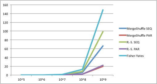
Figure 1: Running times of several random permutation algorithms. Fisher-Yates shuffle, while extremely fast, gets slowed down once permutations are very large. Our parallel MergeShuffle algorithm is consistently faster than all algorithms, although the lead is not yet much compare to the Rao-Sandelius algorithm.

$n$	$10^{5}$	$10^{6}$	$10^{7}$	$10^{8}$
Fisher-Yates	1 631 434	19 550 941	229 329 728	2 628 248 831
MergeShuffle	1 636 560	19 686 051	231 641 075	2 650 387 993
Rao-Sandelius	1 631 519	19 550 449	229 327 120	2 628 251 036
BalancedShuffle	1 889 034	22 046 574

Table 1: Average number of random bits used by our implementation of various random permutation algorithms over 100 trials. (The current implementation of BalancedShuffle were in Python rather than C, and are prohibitively slow on larger permutations, but preliminary results show that it converges to an improved number of random bits.)

Appendix A Code Listing for the MergeSort algorithm

We reproduce here the most part of our algorithm, with some OpenMP [7, 4] hints. The full code can be obtained at https://github.com/axel-bacher/mergeshuffle

A.1 The merge procedure

⬇

// merge together two lists of size m and n-m

void merge(unsigned int *t, unsigned int m, unsigned int n) {

unsigned int *u = t;

unsigned int *v = t + m;

unsigned int *w = t + n;

// randomly take elements of the first and second list according to flips

while(1) {

if(random_bit()) {

if(v == w) break;

swap(u, v ++);

} else

if(u == v) break;

u ++;

}

// now one list is exhausted, use Fisher-Yates to finish merging

while(u < w) {

unsigned int i = random_int(u - t + 1);

swap(t + i, u ++);

}

}

A.2 The MergeSort algorithm itself

⬇

extern unsigned long cutoff;

void shuffle(unsigned int *t, unsigned int n) {

// select q = 2^c such that n/q <= cutoff

unsigned int c = 0;

while((n >> c) > cutoff) c ++;

unsigned int q = 1 << c;

unsigned long nn = n;

// divide the input in q chunks, use Fisher-Yates to shuffle them

#pragma omp parallel for

for(unsigned int i = 0; i < q; i ++) {

unsigned long j = nn * i >> c;

unsigned long k = nn * (i+1) >> c;

fisher_yates(t + j, k - j);

}

for(unsigned int p = 1; p < q; p += p) {

// merge together the chunks in pairs

#pragma omp parallel for

for(unsigned int i = 0; i < q; i += 2*p) {

unsigned long j = nn * i >> c;

unsigned long k = nn * (i + p) >> c;

unsigned long l = nn * (i + 2*p) >> c;

merge(t + j, k - j, l - j);

}

}

}

References

- [1] Laurent Alonso and René Schott. A parallel algorithm for the generation of a permutation and applications. Theor. Comput. Sci., 159(1):15–28, May 1996.
- [2] R. Anderson. Parallel algorithms for generating random permutations on a shared memory machine. In Proceedings of the Second Annual ACM Symposium on Parallel Algorithms and Architectures, SPAA ’90, pages 95–102, New York, NY, USA, 1990. ACM.
- [3] Axel Bacher, Olivier Bodini, and Alice Jacquot. Efficient random sampling of binary and unary-binary trees via holonomic equations. CoRR, abs/1401.1140, 2014.
- [4] Rohit Chandra. Parallel programming in OpenMP. Morgan Kaufmann, 2001.
- [5] Guojing Cong and David A Bader. An empirical analysis of parallel random permutation algorithms on smps. 2006.
- [6] Artur Czumaj, Przemyslawa Kanarek, Miroslaw Kutylowski, and Krzysztof Lorys. Fast generation of random permutations via networks simulation. Algorithmica, 21(1):2–20, 1998.
- [7] Leonardo Dagum and Rameshm Enon. Openmp: an industry standard api for shared-memory programming. Computational Science & Engineering, IEEE, 5(1):46–55, 1998.
- [8] Luc Devroye. Non-Uniform Random Variate Generation. Springer-Verlag, New York, 1986.
- [9] Luc Devroye and Claude Gravel. Sampling with arbitrary precision. arXiv preprint arXiv:1502.02539, 2015.
- [10] Richard Durstenfeld. Algorithm 235: Random permutation. Communications of the ACM, 7(7):420, 1964.
- [11] Ronald A. Fisher and Frank Yates. Statistical Tables for Biological, Agricultural and Medical Research. 3rd Edition. Edinburgh and London, 13(3):26–27, 1948.
- [12] Philippe Flajolet, Maryse Pelletier, and Michèle Soria. On Buffon Machines and Numbers. In Dana Randall, editor, Proceedings of the Twenty-Second Annual ACM-SIAM Symposium on Discrete Algorithms, SODA 2011, pages 172–183. SIAM, 2011.
- [13] Philippe Flajolet and Robert Sedgewick. Analytic Combinatorics. Cambridge University Press, 2009.
- [14] Jens Gustedt. Randomized permutations in a coarse grained parallel environment. In Proceedings of the Fifteenth Annual ACM Symposium on Parallel Algorithms and Architectures, SPAA ’03, pages 248–249, New York, NY, USA, 2003. ACM.
- [15] Jens Gustedt. Engineering parallel in-place random generation of integer permutations. In Proceedings of the 7th International Conference on Experimental Algorithms, WEA’08, pages 129–141, Berlin, Heidelberg, 2008. Springer-Verlag.
- [16] Torben Hagerup. Fast parallel generation of random permutations. In Proceedings of the 18th International Colloquium on Automata, Languages and Programming, pages 405–416, New York, NY, USA, 1991. Springer-Verlag New York, Inc.
- [17] Te Sun Han and Mamoru Hoshi. Interval Algorithm for Random Number Generation. IEEE Transactions on Information Theory, 43(2):599–611, March 1997.
- [18] Donald E. Knuth and Andrew C. Yao. The complexity of nonuniform random number generation. Algorithms and Complexity: New Directions and Recent Results, pages 357–428, 1976.
- [19] Jérémie Lumbroso. Optimal discrete uniform generation from coin flips, and applications. CoRR, abs/1304.1916, 2013.
- [20] C. R. Rao. Generation of random permutation of given number of elements using random sampling numbers. Sankhya A, 23:305–307, 1961.
- [21] Jean-Luc Remy. Un procédé itératif de dénombrement d’arbres binaires et son application à leur génération aléatoire. ITA, 19(2):179–195, 1985.
- [22] Martin Sandelius. A simple randomization procedure. Journal of the Royal Statistical Society. Series B (Methodological), 24(2):pp. 472–481, 1962.
- [23] P. Sanders. Random permutations on distributed, external and hierarchical memory. Inf. Process. Lett., 67(6):305–309, September 1998.
- [24] Julian Shun, Yan Gu, Guy E. Blelloch, Jeremy T. Fineman, and Phillip B. Gibbons. Sequential random permutation, list contraction and tree contraction are highly parallel. In Proceedings of the Twenty-Sixth Annual ACM-SIAM Symposium on Discrete Algorithms, SODA ’15, pages 431–448. SIAM, 2015.
- [25] Richard P Stanley. Catalan Numbers. Cambridge University Press, 2015.
- [26] John von Neumann. Various techniques used in connection with random digits. Applied Math Series, 12:36–38, 1951.