Plasma turbulence and kinetic instabilities at ion scales
in the expanding solar wind

Abstract

The relationship between a decaying strong turbulence and kinetic instabilities in a slowly expanding plasma is investigated using two-dimensional (2-D) hybrid expanding box simulations. We impose an initial ambient magnetic field perpendicular to the simulation box, and we start with a spectrum of large-scale, linearly-polarized, random-phase Alfvénic fluctuations which have energy equipartition between kinetic and magnetic fluctuations and vanishing correlation between the two fields. A turbulent cascade rapidly develops, magnetic field fluctuations exhibit a power-law spectrum at large scales and a steeper spectrum at ion scales. The turbulent cascade leads to an overall anisotropic proton heating, protons are heated in the perpendicular direction, and, initially, also in the parallel direction. The imposed expansion leads to generation of a large parallel proton temperature anisotropy which is at later stages partly reduced by turbulence. The turbulent heating is not sufficient to overcome the expansion-driven perpendicular cooling and the system eventually drives the oblique firehose instability in a form of localized nonlinear wave packets which efficiently reduce the parallel temperature anisotropy. This work demonstrates that kinetic instabilities may coexist with strong plasma turbulence even in a constrained 2-D regime.

I. Introduction

Turbulence in magnetized weakly collisional space and astrophysical plasmas is a ubiquitous nonlinear phenomenon that allows energy transfer from large to small scales, and, eventually, to plasma particles. Properties of plasma turbulence and its dynamics remain an open challenging problem (Petrosyan et al., 2010; Matthaeus & Velli, 2011). The solar wind constitutes a natural laboratory for plasma turbulence (Bruno & Carbone, 2013; Alexandrova et al., 2013), since it offers the opportunity of its detailed diagnostics. Turbulence at large scales can be described by the magnetohydrodynamic (MHD) approximation, accounting for the dominant nonlinear coupling and for the presence of the ambient magnetic field that introduces a preferred direction (Boldyrev et al., 2011). Around particle characteristic scales the plasma description has to be extended beyond MHD and, at these scales, a transfer of the cascading energy to particles is expected. The solar wind turbulence indeed likely energizes particles: radial profiles of proton temperatures indicate an important heating which is often comparable to the estimated turbulent energy cascade rate (MacBride et al., 2008; Cranmer et al., 2009; Hellinger et al., 2013). This energization proceeds through collisionless processes which may have a feedback on turbulence. In the solar wind the problem is further complicated by a radial expansion which induces an additional damping; turbulent fluctuations decrease due to the expansion as well as due to the turbulent decay. The expansion thus slows down the turbulent cascade (cf., Grappin et al., 1993; Dong et al., 2014)). Furthermore, the characteristic particle scales change with radial distance affecting possible particle energization mechanisms.

Understanding of the complex nonlinear properties of plasma turbulence on particle scales is facilitated via a numerical approach (Servidio et al., 2015; Franci et al., 2015a). Direct kinetic simulations of turbulence show that particles are indeed on average heated by the cascade (Parashar et al., 2009; Markovskii & Vasquez, 2011; Wu et al., 2013; Franci et al., 2015a), and, moreover, turbulence leads locally to complex anisotropic and nongyrotropic distribution functions (Valentini et al., 2014; Servidio et al., 2015). Furthermore, expansion naturally generates particle temperature anisotropies (Matteini et al., 2012). The anisotropic and nongyrotropic features may be a source of free energy for kinetic instabilities. In situ observations indicate existence of apparent bounds on the proton temperature anisotropies which are consistent with theoretical kinetic linear predictions (Hellinger et al., 2006; Hellinger & Trávníček, 2014). These linear predictions have, however, many limited assumptions (Matteini et al., 2012; Isenberg et al., 2013); especially, they assume a homogeneous plasma which is at odds with the presence of turbulent fluctuations. On the other hand, the observed bounds on the proton temperature anisotropy (and other plasma parameters) and enhanced magnetic fluctuations near these bounds (Wicks et al., 2013; Lacombe et al., 2014) indicate that these kinetic instabilities are active even in presence of turbulence.

II. Simulation results

In this letter we directly test the relationship between proton kinetic instabilities and plasma turbulence in the solar wind using a hybrid expanding box model that allows to study self-consistently physical processes at ion scales. In the hybrid expanding box model a constant solar wind radial velocity $v_{sw}$ is assumed. The radial distance $R$ is then $R=R_{0}(1+t/t_{e0})$ where $R_{0}$ is the initial position and $t_{e0}=R_{0}/v_{sw}$ is the initial value of the characteristic expansion time $t_{e}=R/v_{sw}=t_{e0}(1+t/t_{e0})$. Transverse scales (with respect to the radial direction) of a small portion of plasma, co-moving with the solar wind velocity, increase $\propto R$. The expanding box uses these co-moving coordinates, approximating the spherical coordinates by the Cartesian ones (Liewer et al., 2001; Hellinger & Trávníček, 2005). The model uses the hybrid approximation where electrons are considered as a massless, charge neutralizing fluid and ions are described by a particle-in-cell model (Matthews, 1994). Here we use the two-dimensional (2-D) version of the code, fields and moments are defined on a 2-D $x$–$y$ grid $2048\times 2048$; periodic boundary conditions are assumed. The spatial resolution is $\Delta x=\Delta y=0.25d_{p0}$ where $d_{p0}=v_{A0}/\Omega_{p0}$ is the initial proton inertial length ($v_{A0}$: the initial Alfvén velocity, $\Omega_{p0}$: the initial proton gyrofrequency). There are $1,024$ macroparticles per cell for protons which are advanced with a time step $\Delta t=0.05/\Omega_{p0}$ while the magnetic field is advanced with a smaller time step $\Delta t_{B}=\Delta t/10$. The initial ambient magnetic field is directed along the radial, $z$ direction, perpendicular to the simulation plane $\boldsymbol{B}_{0}=(0,0,B_{0})$ and we impose a continuous expansion in $x$ and $y$ directions. Due to the expansion the ambient density and the magnitude of the ambient magnetic field decrease as $\bar{n}\propto\bar{B}\propto R^{-2}$ (the proton inertial length $d_{p}$ increases $\propto R$, the ratio between the transverse sizes and $d_{p}$ remains constant; the proton gyrofrequency $\Omega_{p}$ decreases as $\propto R^{-2}$). A small resistivity $\eta$ is used to avoid accumulation of cascading energy at grid scales; initially we set $\eta=10^{-3}\mu_{0}v_{A0}^{2}/\Omega_{p0}$ ($\mu_{0}$ being the magnetic permittivity of vacuum) and $\eta$ is assumed to be $\propto\bar{n}$. The simulation is initialized with an isotropic 2-D spectrum of modes with random phases, linear Alfvén polarization ($\delta\boldsymbol{B}\perp\boldsymbol{B}_{0}$), and vanishing correlation between magnetic and velocity fluctuation. These modes are in the range $0.02\leq kd_{p}\leq 0.2$ and have a flat one-dimensional (1-D) power spectrum with rms fluctuations $=0.24B_{0}$. For noninteracting zero-frequency Alfvén waves the linear approximation predicts $\delta B_{\perp}\propto R^{-1}$ (Dong et al., 2014). Protons have initially the parallel proton beta $\beta_{p\|}=0.8$ and the parallel temperature anisotropy $A_{p}=T_{p\perp}/T_{p\|}=0.5$ as typical proton parameters in the solar wind in the vicinity of 1 AU (Hellinger et al., 2006; Marsch et al., 2006). Electrons are assumed to be isotropic and isothermal with $\beta_{e}=0.5$ at $t=0$.

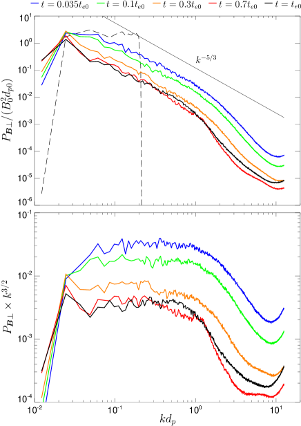
Figure 1.— (top) 1-D PSD $P_{\boldsymbol{B}\perp}$ of the fluctuating magnetic field $B_{\perp}$ perpendicular to the ambient magnetic field and (bottom) $P_{\boldsymbol{B}\perp}$ compensated by $k^{3/2}$ as functions of $k$ at different times. The thin long dashed line shows the initial spectrum and the thin solid line shows a dependence $\propto k^{-5/3}$ for comparison.

The initial random fluctuations rapidly relax and a turbulent cascade develops. Figure 1 shows the evolution of the 1-D power spectral density (PSD) $P_{\boldsymbol{B}\perp}=P_{\boldsymbol{B}\perp}(k)$ of the magnetic field $\boldsymbol{B}_{\perp}$ perpendicular to $\boldsymbol{B}_{0}$. On large scales, the initial flat spectrum evolves to a power law. This large-scale power law remains clearly visible until $t\sim 0.7t_{e0}$ although its slope slowly varies in time, passing from about -3/2 to -5/3 (these estimated slopes are, however, quite sensitive to the chosen range of wave vectors). The variation of large-scale slopes ($kd_{p}\lesssim 1$) is likely connected with the decay of the large scale fluctuations due to the cascade and the expansion as the inertial range is likely quite narrow. This problem is beyond the scope of the present letter and will be a subject of future work (note that a similar steepening is also observed in MHD expanding box simulations, cf., Dong et al., 2014); this letter is mainly focused on ion scales.

Around $kd_{p}\sim 1$ there is a smooth transition in $P_{\boldsymbol{B}\perp}$ separating a the large-scale power law slope and a steeper slope at sub-ion scales (Franci et al., 2015b). The PSD amplitudes decay in time partly due to the expansion and partly to the turbulent damping. Note that there are some indications that the position of the transition shifts to smaller $kd_{p}$ with time/radial distance (compare the blue, green, orange, and red curves in Figure 1); a similar trend is observed for the proton gyroradius since it increases only slightly faster than $d_{p}$. At later times the fluctuating magnetic energy is enhanced at ion scales around $kd_{p}\sim 0.4\div 1$ (compare the red and black curves in Figure 1); this indicates that some electromagnetic fluctuations are generated at later times of the simulation.

Figure 2.— Time evolution of different quantities: (from top to bottom) the fluctuating magnetic field (solid) perpendicular $|\delta B_{\perp}|^{2}$ and (dashed) parallel $|\delta B_{\|}|^{2}$ with respect to $\boldsymbol{B}_{0}$ (the dotted line shows the linear prediction for the zero-frequency Alfvén waves); the average squared parallel current $\langle j_{z}^{2}\rangle$; the parallel $T_{p\|}$ (solid line) and perpendicular $T_{p\perp}$ (dashed line) proton temperatures (the $\|$ and $\perp$ directions are here with respect to the local magnetic field; the dotted lines denote the corresponding CGL predictions); (solid) the nonlinear eddy turnover time $t_{nl}$ at $kd_{p}=1$ (dotted) the expansion time $t_{e}$, and (dashed) the linear time $t_{l}$ for the oblique firehose instability.

Figure 2 summarizes the evolution of the simulated system which goes through three phases. During the first phase the system relaxes from the initial conditions and turbulence develops; the level of magnetic fluctuations increases at the expense of proton velocity fluctuations. The fluctuating magnetic field $\delta B_{\perp}/\bar{B}$ reaches the maximum at about $t\sim 0.008t_{e0}$. During this phase a parallel current $j_{z}$ is generated, $\langle j_{z}^{2}\rangle$ normalized to $\bar{B}^{2}/d_{p}^{2}$ reaches a maximum at $t\sim 0.035t_{e0}$ indicating a presence of a well developed turbulent cascade (Mininni & Pouquet, 2009; Valentini et al., 2014). After that the system is dominated by a decaying turbulence, the fluctuating magnetic field initially decreases faster than $\bar{B}$ till about $0.3t_{e0}$.

During the second phase protons are heated. For negligible heat fluxes, collisions, and fluctuations, one expects the double adiabatic behavior or CGL (Chew et al., 1956; Matteini et al., 2012): the parallel and perpendicular temperatures (with respect to the magnetic field) are expected to follow $T_{p\perp}\propto\bar{B}$ and $T_{p\|}=\mathrm{const.}$, respectively. $T_{p\perp}$ decreases slower than $\bar{B}$ during the whole simulation, protons are heated in the perpendicular direction while in the parallel direction the heating lasts till about $t\sim 0.25t_{e0}$ whereas afterwards protons are cooled. The parallel and perpendicular heating rates could be estimated as (cf., Verscharen et al., 2015):

$$Q_{\|}=\frac{\bar{n}^{3}k_{B}}{\bar{B}^{2}}\frac{\mathrm{d}}{\mathrm{d}t}\left(\frac{T_{\|}\bar{B}^{2}}{\bar{n}^{2}}\right)\ \mathrm{and}\ Q_{\perp}=\bar{n}k_{B}\bar{B}\frac{\mathrm{d}}{\mathrm{d}t}\left(\frac{T_{\perp}}{\bar{B}}\right).$$ (1)

A more detailed analysis indicates that between $t=0.1t_{e0}$ and $t=0.7t_{e0}$ the parallel heating rate $Q_{\|}$ smoothly varies from about $0.2Q_{e}$ and $-0.2Q_{e}$, whereas $Q_{\perp}$ is about constant $\sim 0.2Q_{e}$; here $Q_{e}=\bar{n}k_{B}T/t_{e}$. In total, protons are heated till $t\sim 0.7t_{e0}$ and the heating reappears near the end of the simulation $t\gtrsim 0.95t_{e0}$. Note that the perpendicular heating rate is a nonnegligible fraction of that observed in the solar wind where $Q_{\perp}\approx 0.6Q_{e}$ (Hellinger et al., 2013); however, the proton heating in 2D hybrid simulations is typically quite sensitive to the used electron equation of state (Parashar et al., 2014) and also to the used resistivity and the number of particles per cell (Franci et al., 2015a). The turbulent heating is, however, not sufficient to overcome the expansion-driven perpendicular cooling as in the solar wind (Matteini et al., 2007). During the third phase, $t\gtrsim 0.7t_{e0}$, there is an enhancement of the parallel cooling and perpendicular heating which cannot be ascribed to the effect of the turbulent activity. For a large parallel proton temperature anisotropy a firehose instability is expected. The presence of such an instability is supported by the fact that the fluctuating magnetic field increases (with respect to the linear prediction) suggesting a generation of fluctuating magnetic energy at the expense of protons. To analyze the role of different processes in the system we estimate their characteristic times (Matthaeus et al., 2014). The bottom panel of Figure 2 compares the turbulent nonlinear eddy turnover time $t_{nl}=k^{-3/2}(P_{\boldsymbol{B}\perp}(k)/\mu_{0}m_{p})^{-1/2}$ at $kd_{p}=1$ (cf., Matthaeus et al., 2014), the expansion time $t_{e}$, and the linear time $t_{l}$ of the oblique firehose (Hellinger & Matsumoto, 2000, 2001) estimated as $t_{l}=1/\gamma_{m}$, where $\gamma_{m}$ is the maximum growth rate calculated from the average plasma properties in the box assuming bi-Maxwellian proton velocity distribution functions (Hellinger et al., 2006). The expansion time $t_{e}$ is much longer than $t_{nl}$ at $kd_{p}=1$ (as well as at the injection scales). The expanding system becomes theoretically unstable with respect to the oblique firehose around $t\sim 0.47t_{e0}$ but clear signatures of a fast proton isotropization and of a generation of enhanced magnetic fluctuations appear later $t\gtrsim 0.7t_{e0}$. This is about the time when the linear time becomes comparable to the nonlinear time at ion scales. After that, $t_{l}\Omega_{p}$ slightly increases as a result of a saturation of the firehose instability whereas $t_{nl}\Omega_{p}$ at $kd_{p}=1$ is about constant (note that $\Omega_{p}$ decreses as $R^{-2}$). This may indicate that the instability has to be fast enough to compete with turbulence; however, the 2-D system has strong geometrical constraints. Also the stability is governed by the local plasma properties. Figure 3 shows the evolution of the system in the plane $(\beta_{p\|},A_{p})$. During the evolution, a large spread of local values in the 2-D space $(\beta_{p\|},A_{p})$ develops. Between $t\simeq 0.1t_{e0}$ and $t\simeq 0.65t_{e0}$ the average quantities evolve in time following $\langle A_{p}\rangle\propto\langle\beta_{p\|}\rangle^{-0.86}$. This anticorrelation is qualitatively similar to in situ Helios observations between 0.3 and 1 AU (Matteini et al., 2007). During the third stage, when the strong parallel temperature anisotropy is reduced, both local and average values of $\beta_{p\|}$ and $A_{p}$ appear to be bounded by the linear marginal stability conditions of the oblique firehose (Hellinger & Trávníček, 2008), although relatively large theoretical growth rates $\gamma_{m}\sim 0.1\Omega_{p}$ are expected.

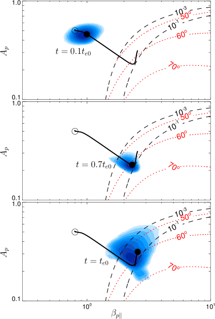
Figure 3.— Simulated data distribution in the plane $(\beta_{p\|},A_{p})$ at different times. The empty circles give the initial condition whereas the solid circles denote the average values. The solid lines show the evolution of the average values. The dashed contours show the maximum growth rate $\gamma_{m}$ (in units of $\Omega_{p}$) of the oblique firehose instability as a function of $\beta_{p\|}$ and $A_{p}$. The dotted contours display the corresponding angle of propagation of the most unstable mode.

The evolution in the real space is shown in Figure 4 which shows the magnitude of the perpendicular fluctuating magnetic field $\delta B_{\perp}$ and the proton temperature anisotropy $A_{p}$ at different times (see also the movie which combines the evolution in Figures 3 and 4). The modes with initially random phases rapidly form vortices and current sheets. Despite the overall turbulent heating a strong temperature anisotropy $T_{p\perp}<T_{p\|}$ develops owing to the expansion and a firehose-like activity develops in a form of localized waves/filaments with enhanced $\delta B_{\perp}$. These fluctuations appear in regions between vortices where $B_{\perp}/\bar{B}$ is enhanced, i.e., in places where the angle between the simulation plane and the local magnetic field $\theta_{B}$ ($\approx\arccos B_{\perp}/\bar{B}$) is less oblique (reaching $\sim 60^{\mathrm{o}}$ and below). This is in agreement with the theoretical expectations, while the oblique firehose is unstable for moderately oblique wave vectors with respect to the magnetic field near threshold, further away from threshold the unstable modes become more oblique (see Figure 3) and these oblique angles are locally available between vortices where we observe the enhanced level of magnetic fluctuations. These geometrical factors may be responsible for the late appearance of the instability (but constraints on the instability time scales imposed by the turbulent non-linearities are likely also important). The localized wave packets are Alvénic, have wavelengths of the order of $10d_{p}$ and propagate with a phase velocity about $0.1v_{A}$ in agreement with expectation for the nonlinear phase of the oblique firehose. Furthermore, the parallel temperature anisotropy is strongly reduced in their vicinity. These Alvénic wave packets are responsible for the enhanced level of the magnetic PSD at ion scales seen in Figure 1.

For a linear instability it is expected that the magnetic fluctuations increase exponentially in time during its initial phase (except when the growth time is comparable to the expansion time, cf., Tenerani & Velli, 2013). Figure 2 however shows that the overall magnetic fluctuations $\delta B_{\perp}/\bar{B}$ (with respect to the linear prediction) and $\delta B_{\|}/\bar{B}$ increase rather slowly (secularly) in time for $t\gtrsim 0.7t_{e}$. This behavior is expected for a long time evolution in a forced system after the saturation (cf., Matteini et al., 2006; Rosin et al., 2011; Kunz et al., 2014). An additional analysis indicates that the expected exponential growth is indeed seen in the simulation but only locally both in space and time. This exponential growth is obscured by the turbulent fluctuations and, furthermore, it is blurred out due to the averaging over the simulation box in the global view of Figure 2.

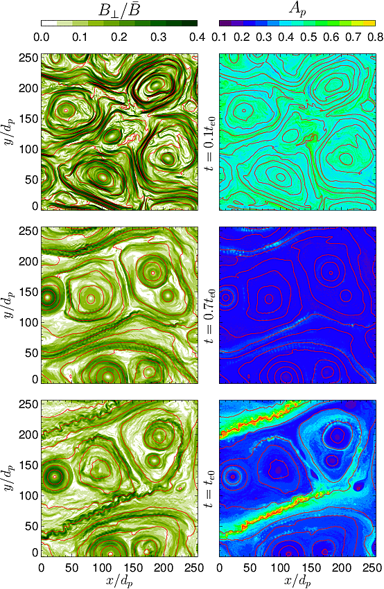
Figure 4.— Color scale plots of (left) $\delta B_{\perp}$ and (right) $A_{p}$ as functions of $x$ and $y$ for (top) $t=0.1t_{e0}$, (middle) $t=0.7t_{e0}$, and (bottom) $t=t_{e0}$. The solid lines show selected (projected) magnetic field lines. Only a quarter of the simulation box is shown.

On the microscopic level the firehose activity leads to an efficient scattering from parallel to perpendicular direction of protons in the velocity space. Figure 5 shows the evolution of the proton velocity distribution function $f=f(v_{\|},v_{\perp})$ averaged over the simulation box. While turbulence leads locally to a complex proton distribution functions (Valentini et al., 2014; Servidio et al., 2015, cf.,) the average proton distribution function during the first two phases remain relatively close to a bi-Maxwellian shape (Figure 5, top panel). During the third phase there appear clear signatures of the cyclotron diffusion (for protons with $v_{\|}\gtrsim v_{A}$) as expected for the oblique firehose instability (Hellinger & Trávníček, 2008).

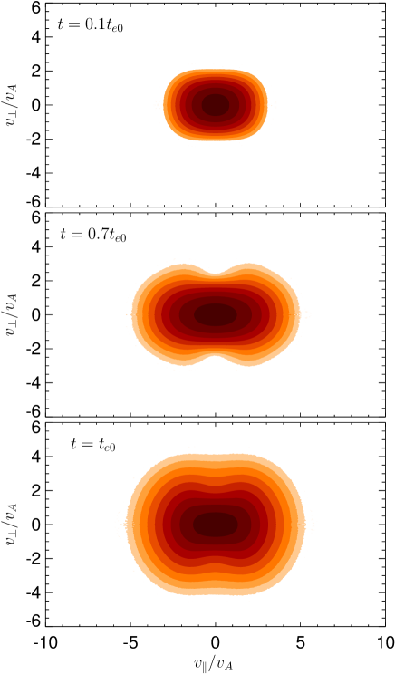
Figure 5.— Average proton velocity distribution function $f$ as a function of parallel and perpendicular velocities $v_{\|}$ and $v_{\perp}$ (with respect to the local magnetic field) for for (top) $t=0.1t_{e0}$, (middle) $t=0.7t_{e0}$, and (bottom) $t=t_{e0}$.

III. Discussion

Using 2-D hybrid simulations we investigated the evolution of turbulence in a slowly expanding plasma. The numerical model shows that the turbulent heating is not sufficient to overcome the expansion driven cooling and that the oblique firehose becomes active for a sufficiently large parallel proton temperature anisotropy and for sufficiently oblique angles of propagation.

While the modeled expansion is about ten times faster than in the solar wind, the ratio between the expansion and the nonlinear eddy turnover time scales is quite realistic: $t_{e}/t_{nl}\approx 1000$ at $kd_{p}=1$ for $t\gtrsim 0.7t_{e}$ which is about four times smaller than that of the solar wind with similar plasma parameters at 1 AU (Matthaeus et al., 2014). Note also that a similar evolution is observed for many different plasma and expansion parameters.

In the present case, both turbulence and the 2-D geometry constraints strongly affect the firehose instability and there are indications that firehose has an influence on turbulence (the mixed third-order structure functions (Verdini et al., 2015) are enhanced due to the firehose activity suggesting a stronger cascade rate). The problem of the interaction between turbulence and kinetic instabilities requires further work; three-dimensional simulations are needed to investigate the interplay between turbulence and instabilities as usually the most unstable modes are parallel or moderately oblique with respect to the ambient magnetic field; in the present case the parallel firehose (Gary et al., 1998; Matteini et al., 2006) would be the dominant instability but the 2-D constraints strongly inhibit it. On the other hand, numerical simulations indicate that the oblique firehose plays an important role in constraining the proton temperature anisotropy in the expanding solar wind even in the case when the parallel firehose is dominant (Hellinger & Trávníček, 2008). Nevertheless, the present work for the first time clearly demonstrates that kinetic instabilities may coexist with strong plasma turbulence and bound the plasma parameter space.

References

- Alexandrova et al. (2013) Alexandrova, O., Chen, C. H. K., Sorriso-Valvo, L., Horbury, T. S., & Bale, S. D. 2013, SSRv, 178, 101
- Boldyrev et al. (2011) Boldyrev, S., Perez, J. C., Borovsky, J. E., & Podesta, J. J. 2011, ApJL, 741, L19
- Bruno & Carbone (2013) Bruno, R., & Carbone, V. 2013, LRSP, 10, 2
- Chew et al. (1956) Chew, G. F., Goldberger, M. L., & Low, F. E. 1956, Proc. R. Soc. London, A236, 112
- Cranmer et al. (2009) Cranmer, S. R., Matthaeus, W. H., Breech, B. A., & Kasper, J. C. 2009, ApJ, 702, 1604
- Dong et al. (2014) Dong, Y., Verdini, A., & Grappin, R. 2014, ApJ, 793, 118
- Franci et al. (2015a) Franci, L., Landi, S., Matteini, L., Verdini, A., & Hellinger, P. 2015a, ApJ, arXiv:1506.05999
- Franci et al. (2015b) Franci, L., Verdini, A., Matteini, L., Landi, S., & Hellinger, P. 2015b, ApJL, 804, L39
- Gary et al. (1998) Gary, S. P., Li, H., O’Rourke, S., & Winske, D. 1998, JGR, 103, 14567
- Grappin et al. (1993) Grappin, R., Velli, M., & Mangeney, A. 1993, PhRvL, 70, 2190
- Hellinger & Matsumoto (2000) Hellinger, P., & Matsumoto, H. 2000, JGR, 105, 10519
- Hellinger & Matsumoto (2001) —. 2001, JGR, 106, 13215
- Hellinger & Trávníček (2005) Hellinger, P., & Trávníček, P. 2005, JGR, 110, A04210
- Hellinger & Trávníček (2008) —. 2008, JGR, 113, A10109
- Hellinger et al. (2006) Hellinger, P., Trávníček, P., Kasper, J. C., & Lazarus, A. J. 2006, GRL, 33, L09101
- Hellinger & Trávníček (2014) Hellinger, P., & Trávníček, P. M. 2014, ApJL, 784, L15
- Hellinger et al. (2013) Hellinger, P., Trávníček, P. M., Štverák, Š., Matteini, L., & Velli, M. 2013, JGR, 118, 1351
- Isenberg et al. (2013) Isenberg, P. A., Maruca, B. A., & Kasper, J. C. 2013, ApJ, 773, 164
- Kunz et al. (2014) Kunz, M. W., Schekochihin, A. A., & Stone, J. M. 2014, PhRvL, 112, 205003
- Lacombe et al. (2014) Lacombe, C., Alexandrova, O., Matteini, L., Santolík, O., Cornilleau-Wehrlin, N., Mangeney, A., de Conchy, Y., & Maksimovic, M. 2014, ApJ, 795, 5
- Liewer et al. (2001) Liewer, P. C., Velli, M., & Goldstein, B. E. 2001, JGR, 106, 29261
- MacBride et al. (2008) MacBride, B. T., Smith, C. W., & Forman, M. A. 2008, ApJ, 679, 1644
- Markovskii & Vasquez (2011) Markovskii, S. A., & Vasquez, B. J. 2011, ApJ, 739, 22
- Marsch et al. (2006) Marsch, E., Zhao, L., & Tu, C.-Y. 2006, Ann. Geophys., 24, 2057
- Matteini et al. (2012) Matteini, L., Hellinger, P., Landi, S., Trávníček, P. M., & Velli, M. 2012, SSRv, 172, 373
- Matteini et al. (2007) Matteini, L., Landi, S., Hellinger, P., Pantellini, F., Maksimovic, M., Velli, M., Goldstein, B. E., & Marsch, E. 2007, GRL, 34, L20105
- Matteini et al. (2006) Matteini, L., Landi, S., Hellinger, P., & Velli, M. 2006, JGR, 111, A10101
- Matthaeus & Velli (2011) Matthaeus, W. H., & Velli, M. 2011, SSRv, 160, 145
- Matthaeus et al. (2014) Matthaeus, W. H., et al. 2014, ApJ, 790, 155
- Matthews (1994) Matthews, A. 1994, JCoPh, 112, 102
- Mininni & Pouquet (2009) Mininni, P. D., & Pouquet, A. 2009, PhRvE, 80, 025401
- Parashar et al. (2009) Parashar, T. N., Shay, M. A., Cassak, P. A., & Matthaeus, W. H. 2009, PhPl, 16, 032310
- Parashar et al. (2014) Parashar, T. N., Vasquez, B. J., & Markovskii, S. A. 2014, PhPl, 21, 022301
- Petrosyan et al. (2010) Petrosyan, A., et al. 2010, SSRv, 156, 135
- Rosin et al. (2011) Rosin, M. S., Schekochihin, A. A., Rincon, F., & Cowley, S. C. 2011, MNRAS, 413, 7
- Servidio et al. (2015) Servidio, S., Valentini, F., Perrone, D., Greco, A., Califano, F., Matthaeus, W. H., & Veltri, P. 2015, JPlPh, 81, 325810107
- Tenerani & Velli (2013) Tenerani, A., & Velli, M. 2013, JGR, 118, 7507
- Valentini et al. (2014) Valentini, F., Servidio, S., Perrone, D., Califano, F., Matthaeus, W. H., & Veltri, P. 2014, PhPl, 21, 082307
- Verdini et al. (2015) Verdini, A., Grappin, R., Hellinger, P., Landi, S., & Müller, W. C. 2015, ApJ, 804, 119
- Verscharen et al. (2015) Verscharen, D., Chandran, B. D. G., Bourouaine, S., & Hollweg, J. V. 2015, ApJ, 806, 157
- Wicks et al. (2013) Wicks, R. T., Matteini, L., Horbury, T. S., Hellinger, P., & Roberts, A. D. 2013, in Proc. 13th Int. Solar Wind Conf., Vol. 1539 (AIP), 303–306
- Wu et al. (2013) Wu, P., Wan, M., Matthaeus, W. H., Shay, M. A., & Swisdak, M. 2013, PhRvL, 111, 121105