ATLAS – I. Third Release of 1.4 GHz Mosaics and Component Catalogues

Abstract

We present the third data release from the Australia Telescope Large Area Survey (ATLAS). These data combine the observations at $1.4\,$GHz before and after upgrades to the Australia Telescope Compact Array reaching a sensitivity of $14\,\mu$Jy beam^-1 in 3.6  deg² over the Chandra Deep Field South (CDFS) and of $17\,\mu$Jy beam^-1 in 2.7  deg² over the European Large Area ISO Survey South 1 (ELAIS-S1). We used a variety of array configurations to maximise the $uv$ coverage resulting in a resolution of 16 by 7 arcsec in CDFS and of 12 by 8 arcsec in ELAIS-S1. After correcting for peak bias and bandwidth smearing, we find a total of 3034 radio source components above $5\sigma$ in CDFS, of which 514 (17 per cent) are considered to be extended. The number of components detected above $5\sigma$ in ELAIS-S1 is 2084, of which 392 (19 per cent) are classified as extended. The catalogues include reliable spectral indices ($\Delta\alpha<0.2$) between 1.40 and 1.71 GHz for $\sim 350$ of the brightest components.

1 Introduction

Large multiwavelength surveys are indispensable for understanding galaxy formation and evolution. Radio wavelengths are valuable in providing an obscuration-independent tracer of star formation and active galactic nucleus (AGN) activity. However, most radio surveys so far have either covered only small areas, thus suffering from sample and cosmic variance, and missing intrinsically rare objects, or cover wide areas but are relatively insensitive, and therefore miss the most active epochs of galaxy formation. In particular, most wide radio surveys have not had sufficient sensitivity to detect normal star formation activity in any but the most nearby galaxies, limiting their ability to contribute to our understanding of the cosmic evolution of galaxies. Another important requisite to maximising the astrophysical value of a survey at any wavelength is to maximise the overlap with other wavelengths.

Here we present the third data release of the Australia Telescope Large Area Survey (ATLAS), which covers $\sim 6$  deg² to an rms depth of $\sim 15\,\mu$Jy beam^-1. The ATLAS survey area consists of two regions centred on the Chandra Deep Field South (CDFS; Giacconi et al., 2001) and the European Large Area ISO Survey - South 1 (ELAIS-S1; Oliver et al., 2000). These two fields were carefully chosen to coincide with areas imaged by the Spitzer Wide-area Infrared Extragalactic Survey (SWIRE; Lonsdale et al., 2003) program, so that infrared and optical data are available for most of the radio objects. They also encompass the well-studied Great Observatories Origins Deep Survey (GOODS) field in CDFS (Giavalisco et al., 2004).

These two areas have since been the target of many other deep multi-wavelength surveys, such as the 4 Ms X-ray survey from Chandra (Xue et al., 2011), the Spitzer Extragalactic Representative Volume Survey (SERVS; Mauduit et al., 2012), the VISTA Deep Extragalactic Observations (VIDEO; Jarvis et al., 2013) survey and the Herschel Multi-tiered Extragalactic Survey (HERMES; Oliver et al., 2012) as well as spectroscopic and photometric redshift surveys, including the PRIsm MUlti-object Survey (PRIMUS; Coil et al., 2011; Cool et al., 2013), the FourStar Galaxy Evolution Survey (zFOURGE; Spitler et al., 2012), the ATLAS spectroscopy program (Mao et al., 2012) and the new OzDES spectroscopy program (Lidman et al., in preparation), making them some of the best-studied fields in the sky.

The first ATLAS data release (DR1: Norris et al., 2006; Middelberg et al., 2008) surveyed these two fields in CDFS and ELAIS-S1 to a typical rms of 36 and $29\,\mu$Jy beam^-1 respectively. The second data release (DR2: Hales et al., 2014a, b) surveyed them to a typical rms of $30\,\mu$Jy beam^-1, addressing a number of sources of systematic error in DR1 and for the first time presenting ATLAS polarisation results. Here in DR3 we report a further improvement to respective rms sensitivities of 14 and $17\,\mu$Jy beam^-1.

Minimising the rms noise is critical, because deep radio surveys such as ATLAS probe flux densities approaching the point where star-forming galaxies start to dominate the radio sky. Surveys of radio sources with flux densities greater than 1 mJy are typically dominated by AGNs, but sources at lower flux densities are increasingly driven by star formation activity (e.g. Seymour et al., 2008; Smolčić et al., 2008; Bonzini et al., 2013). Since star-forming galaxies also dominate non-radio surveys, the fraction of optical/IR galaxies detected at radio wavelengths rises sharply with decreasing flux density, yielding an extinction-free measure of star formation rate.

The key science goals of ATLAS are:

• To determine the relative contribution of starbursts and AGN to the overall energy density of the universe, and the relationship between AGN and star-forming activity. Particularly interesting are composite galaxies in which a radio AGN lies buried within a host galaxy whose optical/infrared spectrum or SED appears to be that of a star-forming galaxy.

• To test whether the far-infrared-radio correlation changes with redshift or with other galaxy properties. Once calibrated, this correlation will be an effective method to measure the star formation history of the Universe.

• To trace the radio luminosity function to a high redshift (z $\sim$ 1) for moderate-power sources, and measure the differential 20 cm source count to a flux density limit of $\sim 100$ $\mu\mathrm{Jy}$ to a high precision.

• To explore regions of parameter space, corresponding to a large area of sky surveyed at high sensitivity at radio, mid-infrared, and far-infrared wavelengths, to discover rare but important objects, such as short-lived phases in galaxy evolution.

A supplementary but important goal is to act as a pathfinder for the Evolutionary Map of the Universe (EMU; Norris et al., 2011) survey, which will use the new Australian SKA Pathfinder (ASKAP; Johnston et al., 2007, 2008; DeBoer et al., 2009) telescope to make a deep ($10\,\mu$Jy beam^-1 rms) radio continuum survey of the entire Southern Sky, extending as far North as $+30^{\circ}$. EMU will cover roughly the same fraction (75%) of the sky as the benchmark NVSS survey (Condon et al., 1998), but will be 45 times more sensitive, and will have an angular resolution (10 arcsec) 4.5 times higher. EMU is expected to generate a catalogue of about 70 million galaxies, compared to the $\sim$ 2.5 million sources currently known at all radio frequencies. Since EMU will have a similar resolution to ATLAS, we are using ATLAS to test many of the technical and scientific processes for EMU. In addition, we will use optical spectroscopy of ATLAS galaxies to train the photometric redshift algorithms for EMU.

Throughout this paper we define a radio ‘component’ as a discrete region of radio emission identified in the source extraction process. We define a radio ‘source’ as one or more radio components that appear to be physically connected to one host galaxy. Thus, we count a classical triple radio-loud source as being a radio source consisting of three radio components, but count a pair of interacting starburst galaxies as being two sources, each with one radio component (providing of course that the angular separation between the starburst galaxies is large enough for them to be resolved).

This paper (Paper I) is primarily concerned with describing the survey and presenting the component catalogue. Paper II (Banfield et al. 2015, in preparation) will extract the component counts and explore the distribution of spectral indices, and Paper III (Norris et al. 2015, in preparation) will group the components into sources with optical/infrared identifications. Subsequent papers in the series will address the individual science goals of ATLAS.

This paper is organised as follows. Section 2 describes the observations, calibration and imaging, and Section 3 details the corrections made to the final image prior to component extraction. Section 4 describes the component extraction process and presents the ATLAS DR3 component catalogue. We summarise our results in Section 5.

Throughout this paper we assume a Hubble constant of $71\,{\rm km}\,{\rm s}^{-1}{\rm Mpc}^{-1}$, and matter and cosmological constant density parameters of $\Omega_{\rm M}=0.27$ and $\Omega_{\rm\Lambda}=0.73$, and assume the convention for spectral index, $\alpha$, where $S\propto\nu^{\alpha}$.

2 Observations, Calibration and Imaging

2.1 Target Fields

Table 1: Available radio data and observations in CDFS and ELAIS-S1. Listed is the wavelength, telescope and survey where applicable, area overlap with the data presented in this paper, sensitivity, angular resolution and reference.

Field	Wavelength	Survey/	Overlapping	Sensitivity	Resolution	Reference
		Instrument	Area (deg2)	($\mu$Jy/bm)	( arcsec)
CDFS	$15\,$mm ($20\,$GHz)	ATCA	2.50	$300$	$29.1\times 21.9$	Franzen et al. (2014)
	$6\,$cm ($5.5\,$GHz)	ATLAS/ATCA	0.25	$12$	$4.0\times 2.0$	Huynh et al. (2012)
	$13\,$cm ($2.3\,$GHz)	ATLAS/ATCA	3.57	$80$	$57.2\times 22.7$	Zinn et al. (2012)
	$21\,$cm ($1.4\,$GHz)	VLA	$0.33$	$7.4$	$2.8\times 1.6$	Miller et al. (2013)
	$21\,$cm ($1.4\,$GHz)	ATLAS/ATCA	3.57	$40$	$11\times 5$	Norris et al. (2006)
	$21\,$cm ($1.4\,$GHz)	ATLAS/ATCA	3.57	$30$	$12\times 6$	Hales et al. (2014a)
	$21\,$cm ($1.4\,$GHz)	NVSS/VLA	3.57	$450$	45	Condon et al. (1998)
	$92\,$cm (325 MHz)∗	GMRT	3.57	$100$	$7.1\times 10.8$	Afonso et al. (2007)
	$1.25-3.75$ m ($80-240$ MHz)∗	GLEAM	3.57	3000	150	Wayth et al. (2015)
	$1.5-3$ m ($104-196$ MHz)	MWACS	3.57	40000	180	Hurley-Walker et al. (2014)
	2 m (150 MHz)	TGSS/GMRT	3.57	$5-7$ mJy	20	Sirothia et al. (2012)
	4 m (74 MHz)	VLSS/VLA	3.57	0.1 Jy	80	Cohen et al. (2007)
ELAIS-S1	$13\,$cm ($2.3\,$GHz)	ATLAS/ATCA	2.70	$70$	$33.6\times 19.9$	Zinn et al. (2012)
	$21\,$cm ($1.4\,$GHz)	ATLAS/ATCA	2.70	$30$	$10.3\times 7.2$	Middelberg et al. (2008)
	$21\,$cm ($1.4\,$GHz)	ATLAS/ATCA	2.70	$30$	$12\times 6$	Hales et al. (2014a)
	$36\,$cm ($843\,$MHz)	MOST	2.70	$600$	$62\times 43$	Randall et al. (2012)
	$50\,$cm ($610\,$MHz)	GMRT	3.30	100	$10\times 5$	Intema (2014)
	$2\,$m ($150\,$MHz)	TGSS/GMRT	2.70	$5-7$ mJy	20	Sirothia et al. (2012)
	$1.25-3.75$ m ($80-240$ MHz)∗	GLEAM	2.70	3000	150	Wayth et al. (2015)
	$1.5-3$ m ($104-196$ MHz)	MWACS	2.70	40000	180	Hurley-Walker et al. (2014)
	∗ Data yet to be released.

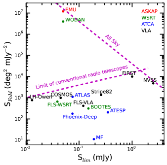
Figure 1: Comparison of ATLAS with the following $1.4\,$GHz surveys: the Evolutionary Map of the Universe (EMU; Norris et al., 2011) survey, the Westerbork Observations of the Deep APERTIF Northern-Sky (WODAN; Röttgering et al., 2010) survey, the NRAO VLA Sky Survey (NVSS; Condon et al., 1998), the Faint Images of the Radio Sky Twenty Centimetres (FIRST; Becker, White & Helfand, 1995) survey, the Phoenix Deep Survey (Hopkins et al., 2003), the Australia Telescope ESO Slice Project (ATESP; Prandoni et al., 2000) survey and surveys of the Bootes field by de Vries et al. (2002), the Marano Field by Gruppioni et al. (1997), the Lockman Hole by Owen & Morrison (2008), the COSMOS field by Schinnerer et al. (2007), Stripe 82 of the Sloan Digital Sky Survey by Hodge et al. (2011) and the First-Look Survey region by Morganti et al. (2004) and by Condon et al. (2003). The telescope used to conduct each of the surveys is indicated in the top right. The horizontal axis is the $5\sigma$ detection limit of the surveys in mJy and the vertical axis is the $S_{\mathrm{FoM}}$ factor for surveys in deg² mJy^-2 (see section 2.1 for more detail). The two dashed lines indicate the All Sky limit and the approximate envelope of existing surveys, heavily dependent on available telescope time.

ATLAS covers two regions, each of $\sim 3~{}\mathrm{deg}^{2}$, surrounding CDFS ($\alpha=03^{\rm h}30^{\rm m}16.3^{\rm s}$, $\delta=-28^{\rm o}05^{\prime}12.4^{\prime\prime}$) and ELAIS-S1 ($\alpha=00^{\rm h}33^{\rm m}50.8^{\rm s}$, $\delta=-43^{\rm o}44^{\prime}57.4^{\prime\prime}$). These two fields have previously been observed at $1.4\,$GHz as part of the ATLAS project and are described by Hales et al. (2014a). Both of these fields were originally targeted for radio observations as they overlap with SWIRE which includes infrared and optical data for the majority of the radio objects. Table 1 lists the available radio observations ($74\,$MHz – $20\,$GHz) overlapping the two ATLAS fields.

To compare ATLAS with other existing $1.4\,$GHz surveys shown in Fig. 1, we compile a figure of merit for surveys, $S_{\mathrm{FoM}}$. The goal of a survey is to maximise the area observed and minimise the noise in the image. This is limited by the fact that it takes $T^{2}$ times longer to decrease the thermal noise by a factor of $T$ and $T$ times longer to increase the observing area by a factor of $T$. Therefore, $S_{\mathrm{FoM}}$ is of the form:

$$S_{\mathrm{FoM}}=\frac{\Omega}{(S_{\rm lim})^{2}}\,,$$ (1)

where $\Omega$ is the survey area in square degrees and $S_{\rm lim}$ is the $5\sigma$ detection limit of the survey in mJy. Bunton & Hay (2010) used a similar metric to quantify the survey speed for chequerboard phased array feeds. Of the current 1.4 GHz surveys, FIRST has the largest $S_{\mathrm{FoM}}$ ($1\times 10^{4}\,$deg² mJy^-2). ATLAS has a similar $S_{\mathrm{FoM}}$ (1108 deg² mJy^-2) to LH-Owen, COSMOS and Stripe82, thereby providing among the deepest and widest coverage of radio objects at 1.4 GHz.

We used the Australia Telescope Compact Array (ATCA; Frater, Brooks, & Whiteoak, 1992) at $1.4\,$GHz to observe the two ATLAS fields in all four Stokes parameters ($XX,YY,XY,YX$). During our observing campaign, the ATCA was being upgraded with the Compact Array Broadband Backend (CABB; Wilson et al., 2011) providing a larger instantaneous bandwidth coupled with increased sensitivity of continuum and spectral line observations. At the time of our ATLAS observations, the CABB band provided a $500\,$MHz bandwidth covering $1.3-1.8\,$GHz, split into $1\,$MHz channels.

ATCA project C1967 was allocated 1000 hours distributed over 78 days between 2009 June and 2010 June to extend ATLAS. The observations were spread over the four 6 km array configurations to maximise uv coverage as listed in Table 7. The primary flux and bandpass calibrator PKS 1934-638 ($14.95\,$Jy at $1.380\,$GHz; Reynolds, 1994) was visited at the beginning of each observing run. Two different secondary phase calibrators, PKS 0022-433 for ELAIS-S1 and PKS 0400-319 for CDFS, were observed every 15 minutes throughout the observations to determine the antenna complex gains and polarization leakage correction. We observed the two fields in the standard ATCA mosaic mode with 28 pointings in CDFS and 20 pointings in ELAIS-S1. The 48 pointing centres are listed in Table 8.

2.2 Calibration

We calibrated and edited the uv data using MIRIAD (Sault, Teuben, & Wright, 1995). The standard MIRIAD calibration techniques are optimised for the original ATCA correlator system ($2\times 128\,$MHz bandwidths) and had to be expanded to calibrate the new CABB-enabled bandwidth. We calibrated each day of observations separately following the method outlined below.

We removed channels affected by self-interference due to the 640-MHz clock harmonics and by known radio frequency interference with atlod in MIRIAD using the options birdie and rfiflag. We then restricted the frequencies to the known range of good bandpass response using uvaver to include only data between 1.3 and 1.8 GHz. Calibration of the bandpass was completed using the standard MIRIAD procedure mfcal and we applied the calibration to the secondary calibrator. Automatic flagging of the calibrators was completed using mirflag, setting int=600. This task implements the automatic flagging routine pieflag developed by Middelberg (2006). We also manually flagged the calibrators using uvflag.

The large bandwidth poses an issue with frequency dependent calibration. The standard MIRIAD calibration procedure was altered to deal with the large bandwidth when calibrating the antenna gains and phases and the instrumental polarization. The task gpcal has been updated to allow for calibration over smaller frequency bands instead of over the full CABB band. For our data, we calibrated over $128\,$MHz sections across the band using the option nbins in gpcal. Once the calibration was complete, we copied the solutions to the targets using gpcopy. The target pointings were then flagged using mirflag with int=1200 and further manually flagged with uvflag. The mean integration time per pointing after flagging is $\approx 15$ hours in CDFS and $\approx 9$ hours in ELAIS-S1.

2.3 Imaging

2.3.1 Single Pointing Image Processing

We combined all data for each pointing into one file using uvcat and then each pointing was imaged separately. Since the observations cover a large fractional bandwidth, multifrequency synthesis was used.

Sault & Conway (1999) describe the process of multi-frequency synthesis and how to successfully CLEAN an image. When creating an image over a wide bandwidth, two dirty beam images must be used, as the spectrum of a radio sources is given by

$$I(\nu)=I(\nu_{\rm 0})+\alpha I(\nu_{\rm 0})\frac{\nu-\nu_{\rm 0}}{\nu_{\rm 0}}\ ,$$ (2)

where $I$ is the flux density at frequency $\nu$, $\nu_{\rm 0}$ is the reference frequency and $\alpha$ is the spectral index (Sault & Conway, 1999). The two dirty beams are the synthesised dirty beam and the spectral dirty beam. The dirty image is then represented by

$$I_{\rm D}(l,m)=I(l,m)*B_{\rm 0}(l,m)+(\alpha(l,m)I(l,m))*B_{\rm 1}(l,m)\ ,$$ (3)

where $B_{\rm 0}$ is the synthesised dirty beam, $B_{\rm 1}$ is the spectral dirty beam and $(l,m)$ are the directional cosines (Sault & Conway, 1999). The MIRIAD task invert provides the option of creating the two dirty beams. These two dirty beams are used in the multi-frequency CLEAN task, mfclean, to create the CLEAN component $I$ and $\alpha I$ maps.

Each pointing was CLEANed and self-calibrated separately prior to mosaicking. A model for self-calibration was produced by imaging the full band with uniform weighting and a cell size of 1 arcsec. The band was then split up into four 125 MHz subbands and self-calibration was applied to each subband separately in order to allow for variations in the antenna gains with frequency. Three iterations of phase self-calibration were applied, progressively increasing the number of CLEAN components used to model the sky emission, and hence the total amount of flux included in the model.

The final self-calibrated $uv$ data were then divided into two subbands of $250\,$MHz, imaged separately and adjusted to the reference pointing. Splitting up the data into two subbands serves to improve the accuracy of the primary beam correction. In order to obtain nearly identical synthesised beams for all pointings, individual ‘robust’ weighting factors (Briggs, 1995) were assigned. Pointings in the lower subband typically have a robust weighting factor in the range 0.0–0.5 and in the higher subband 0.4–1.0.

Using robust weighting factors in these ranges was found to minimise the rms noise in the final mosaic. Using higher robust weighting factors – a robust weighting factor of 2 or more corresponds very closely to natural weighting – was found to degrade the image sensitivity, despite the decrease in the theoretical noise level. This probably arises, in large part, from the degradation of the sidelobe levels and beam-shape, which renders the task of CLEANing the image and removing artifacts harder.

The larger beam size obtained when using natural weighting also increases the confusion noise (Condon et al., 2012). The final beam size in ELAIS-S1 is 12.2 by 7.6 arcsec and in CDFS is 16.3 by 6.8 arcsec (see Section 2.4). At a frequency of 1.4 GHz and a resolution of 9.6 arcsec (the geometric mean of the major and minor beam axes in ELAIS-S1), the confusion noise $\sigma_{\mathrm{c}}\approx 3.8~{}\mu$Jy beam^-1. $\sigma_{\mathrm{c}}$ is predicted to vary as $\theta^{10/3}$, where $\theta$ is the beam size. Using a robust weighting factor of 2 for all pointings in ELAIS-S1 results in a final beam size of 17.9 by 11.8 arcsec, for which $\sigma_{\mathrm{c}}\approx 14.9~{}\mu$Jy beam^-1.

When imaging the self-calibrated $uv$ data, the cell size was set to 1.5 arcsec. We CLEANed each pointing down to 5$\sigma$. A 2D elliptical Gaussian fitted to the central region of the dirty beam was used as the restoring beam. The mfs option in restor was used to write a second plane in the output image containing the $\alpha I$ model convolved with the Gaussian beam. The $\alpha I$ plane was subsequently used to perform wideband primary beam correction in linmos (see Section 2.4). The pointing reference for ELAIS-S1 is $\alpha=00^{\rm h}33^{\rm m}50.8^{\rm s}$, $\delta=-43^{\rm o}44^{\prime}57.4^{\prime\prime}$ and for CDFS is $\alpha=03^{\rm h}30^{\rm m}16.3^{\rm s}$, $\delta=-28^{\rm o}05^{\prime}12.4^{\prime\prime}$.

2.3.2 Image Artifacts

Radial spokes are present around bright sources in both fields. We found that these can be effectively removed using amplitude self-calibration. Fig. 2 shows the improvement in dynamic range after amplitude self-calibration around a 1.4 Jy source (NVSS J032836-284147; Condon et al., 1998) in CDFS; the dynamic range (as measured by dividing the peak flux density of the source by the rms in the vicinity of the source) is $\approx 70$ per cent higher after amplitude self-calibration.

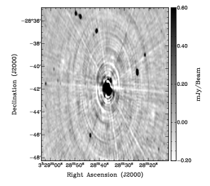
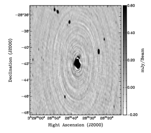
Figure 2: Map of a 1.4 Jy source (NVSS J032836-284147) in CDFS, before (top) and after (bottom) amplitude self-calibration.

We tried to apply amplitude self-calibration to the ATLAS pointings using components with flux density greater than $5\sigma$ to model the sky brightness distribution. This caused the flux densities of sources below approximately 1 mJy to be biased low. The magnitude of the bias was found to increase for sources with decreasing flux density below 1 mJy, reaching $\sim 10$ per cent close to the $5\sigma$ detection limit. We suspect that a considerable amount of flux was missing in the model due to the flat slope of the counts at sub-mJy levels, resulting in the observed bias in the source flux densities. Wieringa et al. (1992) investigated self-calibration methods in use at radio synthesis arrays and found that self-calibration can bias the gains if a significant amount of flux is missing in the model, particularly in cases where the number of antennas is low. Any sources not fully contained in the model tend to get absorbed into the gains and are then reduced in amplitude in the image after self-calibration. Amplitude self-calibration was therefore not used when producing the final images.

Mild artifacts in the form of concentric rings are also visible around the strong source shown in Fig. 2. These limitations are related to difficulties in modelling and calibrating time-dependent effects simultaneously using standard self-calibration techniques, particularly where the source is bright and partially (or fully) resolved. This is primarily due to the east-west nature of ATCA array configurations (i.e. at any point in time only a slice in the $uv$ plane is sampled). Lenc et al. (2009) found that, in the pointing closest to the strong source, these artifacts could be removed by modelling the source in the $uv$ plane with a combination of Gaussians and point-like components, using Difmap (Shepherd, 1997). We did not apply this technique here because it was difficult to automate and it could not handle wideband data.

2.3.3 Addition of Previous ATLAS Data

Previous ATLAS DR2 observations (ATCA Project IDs C1035 and C1241) from Hales et al. (2014a) were combined with our CABB observations to maximise the sensitivity. Information on these observations including observing dates and ATCA array configurations is given in Table 7. The data were combined in the image plane for reasons related to bandwidth smearing, and described in detail in Section 3.2. These data consist of two $128\,$MHz bands centred at 1344 and $1432\,$MHz each containing 16 channels of $8\,$MHz in size. Both bands were imaged together using a similar procedure to the CABB data. The robust weighting factors for the pointings were chosen to yield a similar beam size to that of the CABB data. Pointings typically have a robust weighting factor in the range $-0.1$ – $+0.1$.

Addition of the pre-CABB data results in an improvement in sensitivity of $\approx 20$ per cent and also improves the dynamic range thanks to the increased $uv$ coverage.

2.4 Mosaics

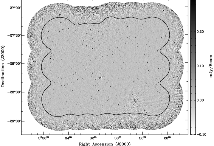
Figure 3: The ATLAS CDFS total intensity mosaic with the linear greyscale set to the range $-100$ to $+300\,\mu$Jy beam^-1. The image projection used is North-celestial-pole (NCP; Greisen, 1983), a projection onto a plane perpendicular to the North Celestial Pole, which is a special case of the orthographic (SIN) projection, often used for east-west radio interferometers. The solid black contour indicates the component catalogue boundary (3.6 $\mathrm{deg}^{2}$) of the mosaic defined by: (1) local rms noise $\leq 100\,\mu$Jy beam^-1; (2) sensitivity loss due to bandwidth smearing $<20$ per cent; and (3) mosaicked primary beam response $\geq 40$ per cent. The pattern of pointings on the sky is identical to that shown in Norris et al. (2006).

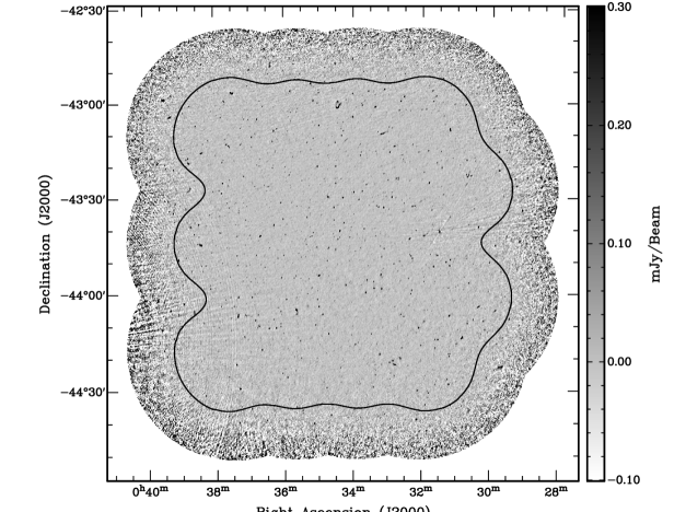
Figure 4: The ATLAS ELAIS-S1 total intensity mosaic with the linear greyscale set to the range $-100$ to $+300\,\mu$Jy beam^-1. The image projection used is NCP. The solid black contour indicates the component catalogue boundary (2.7 $\mathrm{deg}^{2}$) of the mosaic defined by: (1) rms noise $\leq 100\,\mu$Jy beam^-1; (2) sensitivity loss due to bandwidth smearing $<20$ per cent; and (3) mosaicked primary beam response $\geq 40$ per cent. The pattern of pointings on the sky is identical to that shown in Middelberg et al. (2008).

Each pointing was convolved with a Gaussian to obtain an identical synthesised beam across each of the two fields separately. CDFS has a beam size of 16.3 by 6.8 arcsec, with position angle $2\degr$, and ELAIS-S1 a beam size of 12.2 by 7.6 arcsec, with position angle $-11\degr$. A source-free estimate of the noise in each pointing image was obtained as follows: an initial estimate of the noise was obtained by taking the rms within the primary beam full-width at half-maximum (FWHM). To avoid the noise estimate from being affected by real source emission, all pixels outside the range $\pm 3\sigma$ were then flagged and the rms was re-evaluated. This process was repeated a number of times until the noise was found to decrease by less than 10 per cent after removing pixel outliers.

Finally, using linmos, the pointings for each field were corrected for the primary beam and mosaicked together, weighting them by their respective rms noise values; Gaussian primary beam fits for the new 16 cm CABB receivers across the entire frequency range (1.1 to 3.1 GHz) were used and the primary beam response was averaged over the subband as described below. Fig. 3 shows the resulting CDFS total intensity (Stokes $I$) image and Fig. 4 shows the resulting ELAIS-S1 total intensity image.

Due to the wideband nature of the observations there is a discrepancy between the integrated flux density over the band (as returned by MIRIAD) and the monochromatic flux density at the central frequency for any source with a non-zero spectral index. This is essentially due to most sources being best described by a power-law slope across the band rather than a simple linear slope. The integrated flux density for a source with a power-law rather than a linear slope across the band is always going to exceed the monochromatic flux density at the central frequency. For small $\frac{\Delta\nu}{\nu_{0}}$ this effect is small, but increases for wider bands and for a source with an increasingly non-flat spectrum. In our case, for $\alpha=-0.75$, typical of radio sources whose emission is dominated by optically thin synchrotron radiation, a source would have its monochromatic flux density over-estimated by less than 0.5 per cent in each subband, well within the absolute calibration errors.

However, this issue gets more complicated off-axis as the attenuation of the primary beam drops off more rapidly at higher frequencies effectively reducing the sensitivity at higher frequencies. For narrow-band observations with a well known primary beam pattern (which varies with frequency), using the primary beam correction factor at the central frequency is sufficient. For wide-band observations the primary beam correction at this frequency is not truly representative.

To improve the accuracy of the primary beam correction, we used the implementation of wideband primary beam correction in linmos (option bw): the image and primary beam were evaluated at 10 frequencies, the image using the $\alpha I$ plane and the beam using the beam fits across the frequency range. All these images and beams were then used in the standard mosaic equation (see e.g. Sault, Staveley-Smith & Brouw, 1996) to produce the final mosaicked image.

3 Correction of Final Mosaics

3.1 CLEAN Bias

Table 2: Number of simulated sources added to the uv data of one ELAIS-S1 pointing at a given SNR to analyse the CLEAN bias.

$N$	SNR
40	5
15	6
15	7
15	8
15	9
10	10
10	12
5	16
3	20
2	30
1	50
1	100

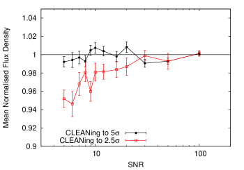
Figure 5: The mean normalised flux density of simulated sources as a function of the SNR. The lines illustrate the CLEAN bias when CLEANing to $5\sigma$ (black line and circles) and $2.5\sigma$ (red line and squares).

CLEAN bias (Condon et al., 1998) is an effect in deconvolution which redistributes flux from point sources to noise peaks in the image, thereby resulting in a systematic underestimation of the flux densities of real sources. As the amount of flux which is taken away from a real source is independent of its flux density, the fractional error this causes is largest for faint sources. The magnitude of the effect will depend on the uv coverage and to what flux density level the images are CLEANed.

In order to analyse the CLEAN bias on the flux density of sources in our ATLAS mosaics, we followed a similar procedure to that outlined in Middelberg et al. (2008). We added 132 point sources at random positions to the $uv$ data of one ELAIS-S1 pointing, except that a simulated source could not lie closer than 1 arcmin from a real source ($>5\sigma$) and any other simulated source. The numbers of sources added with different signal-to-noise ratios (SNRs) are listed in Table 2. We then imaged the data in the same way as the final image (see Section 2.3), extracted the flux density of each simulated source and divided by the injected flux density. This simulation was repeated 30 times to improve the statistical sampling.

The mean normalised flux density of the simulated sources as a function of SNR is shown in Fig. 5. The flux densities of the simulated sources were measured by extracting the map values at the simulated source positions, interpolated between pixels. This was done by calculating the map values on a successively finer grid (up to 128 times finer), by repeated convolution with a Gaussian-graded sinc function (Rees, 1990). At low SNR, the thermal noise will introduce a slight shift in the position of a point source, resulting in an increased likelihood for the peak to lie on top of a positive noise fluctuation. This, in turn, causes the peak flux density of a point source to be biased slightly high; this is known as the peak flux density bias. We chose to measure the flux densities of the simulated sources at their true positions, rather than measure their peak flux densities, to disentangle the peak flux density bias from the CLEAN bias. The peak flux density bias is dealt with separately by the BLOBCAT source finder in Section 4.2.

The black circles in Fig. 5 show the CLEAN bias when CLEANing the images to 5$\sigma$, which typically corresponds to 5000 iterations (the final images were CLEANed to this level). The simulations indicate that a source with an SNR of 5 would have its flux density underestimated by less than 1 per cent as a result of the CLEAN bias, well within the calibration error of 5 per cent (see Section 4.6). We therefore chose not to correct the sources’ flux densities for this effect.

We repeated the simulations CLEANing the images to 2.5$\sigma$ (this typically corresponds to 65000 iterations) to see how the CLEAN bias is affected by the flux density level to which the images are CLEANed. In this case, the CLEAN bias is much more significant as shown by the blue squares in Fig. 5; the CLEAN bias is $\sim$5 per cent for sources with an SNR of 5.

3.2 Bandwidth Smearing

Figure 6: The fraction of the CDFS (solid line) and ELAIS-S1 (dashed line) mosaics at or below a given bandwidth smearing level. The total area of the mosaic ($\Omega_{\rm total}$) is defined where the rms noise level is less than $100\,\mu$Jy beam^-1.

Bandwidth smearing (chromatic aberration) is characterised by a smearing of the visibilities of a point source in the $uv$ plane due to the range of frequency being sampled over a given bandwidth. This results in a decrease in the peak flux density of the source (Condon et al., 1998). The effect on sources in an image is to introduce smearing in the radial direction from the pointing centre, so although the peak flux density is reduced, the integrated flux density remains the same. Bandwidth smearing can cause the peak flux density to fall below the sensitivity threshold, thus rendering it unrecoverable. The magnitude of the effect will depend on the source distance from the pointing centre and the fractional channel bandwidth. The effect of bandwidth smearing is small for CABB data (with 1 MHz channels) but significant for pre-CABB data (with 8 MHz channels) and is the primary cause of the amplitude calibration discrepancy reported by Norris et al. (2006).

In order to analyse the bandwidth smearing in our ATLAS mosaics, we followed a similar procedure to that outlined in Hales et al. (2014a). We modelled the amount of bandwidth smearing to produce simulated images from Hales et al.:

$$\frac{S_{\rm peak}}{S}=\left[1+\frac{2{\rm ln}2}{3}\left(\frac{\Delta\nu_{\rm eff}}{\nu}\frac{d}{B_{\rm proj(\zeta)}}\right)\right]^{-\frac{1}{2}}\ ,$$ (4)

where $S_{\rm peak}$ is the peak flux density of the source, $S$ the integrated flux density of the source, $\Delta\nu_{\rm eff}$ the effective channel bandwidth, $\nu$ the central frequency, $d$ the radial distance from the phase centre and $B_{\rm proj}(\zeta)$ the projected beam FWHM for an elliptical beam. The projected beam FWHM is given by Hales et al.:

$$B_{\rm proj}(\zeta)=\frac{B_{\rm maj}B_{\rm min}}{\sqrt{[B_{\rm maj}{\rm sin}(\zeta-\psi)]^{2}+[B_{\rm min}{\rm cos}(\zeta-\psi)]^{2}}}\ ,$$ (5)

where $\zeta$ is the position angle (East of North) of a source with respect to the phase centre, $B_{\rm maj}$ and $B_{\rm min}$ are the major and minor axes FWHM of the elliptical beam respectively, and $\psi$ is the beam position angle measured East of North.

All of these simulated images were mosaicked together following the method outlined in Section 2.4. The effect of bandwidth smearing on the CDFS and ELAIS-S1 mosaics is shown in Fig. 6. The bandwidth smearing for both mosaics is less than 10 per cent over the great majority of the observational area. Sources’ peak flux densities were corrected for bandwidth smearing, using our maps quantifying the sensitivity loss due to bandwidth smearing, as described in Section 4.2.

4 1.4 GHz Component Catalogue

4.1 Background Noise Map

Figure 7: The fraction of the CDFS (solid line) and ELAIS-S1 (dashed line) mosaics at or below a given rms noise level. The total area of the mosaic ($\Omega_{\rm total}$) is defined where the rms noise level is less than $100\,\mu$Jy beam^-1.

In order to extract sources from the mosaics we require an estimate of the background noise level. The background rms noise of each mosaic was calculated for each pixel following the method described by Franzen et al. (2014). For each pixel, the noise was taken as the rms inside a box of size $2l+1$ centred on the pixel; we chose the half-width of the box, $l$, to be 20 times the beam for both mosaics to minimise the number of spurious detections (Huynh et al., 2012). However, in order to avoid the noise estimate from being affected by real source emission, points were clipped iteratively until convergence at $\pm 3\sigma$ was reached. Fig. 7 shows the fraction of the ATLAS sky at or below a given rms noise level, where the ATLAS sky is defined where the rms noise is less than $100\,\mu$Jy beam^-1. Table 4 gives statistics for the rms noise distribution across the ATLAS sky for the two fields.

Table 3: Statistics for the rms noise distribution across the ATLAS sky (region where the rms noise is less than $100\,\mu$Jy beam^-1) for CDFS and ELAIS-S1.

	CDFS	ELAIS-S1
Mean ($\mu$Jy beam-1)	30	35
Median ($\mu$Jy beam-1)	23	24
Mode ($\mu$Jy beam-1)	14	17

4.2 Source Extraction

We limited the area of the two ATLAS fields for source extraction defined by the union of the following criteria:

1. rms noise $\leq 100\,\mu$Jy beam^-1.

2. sensitivity loss due to bandwidth smearing $<20$ per cent.

3. mosaicked primary beam response $\geq 40$ per cent of the peak response.

Fig. 3 shows the defined area covering 3.6 $\mathrm{deg}^{2}$ of the CDFS mosaic and Fig. 4 shows the defined area covering 2.7 $\mathrm{deg}^{2}$ of the ELAIS-S1 mosaic. The resulting area is primarily defined by the primary beam response.

We extracted source components from the two ATLAS fields using BLOBCAT (Hales et al., 2012), AEGEAN (Hancock et al., 2012), pyBDSM and the AMI SOURCE_FIND software (AMI Consortium: Franzen et al., 2011). When using BLOBCAT, AEGEAN and pyBDSM, we searched both mosaics down to an SNR $\geq 4$ in order to include all sources with fitted peak SNRs $\geq 5$. Sources with fitted peak SNRs $<5$ were removed manually from the output component lists. When running SOURCE_FIND on the two mosaics, a detection threshold of 5$\sigma$ was used since the detection threshold is automatically lowered to ensure that all sources with fitted peak SNRs $\geq 5$ are included. We compared the source finders by locating the corresponding counterparts to within 20 arcsec. The difference between the four source finders for our work is negligible. However, we chose BLOBCAT over the other source finders as BLOBCAT takes into consideration bandwidth smearing and peak bias. A more detailed analysis of the source finders is beyond the scope of this paper but is discussed by Hopkins et al. (2014), submitted.

Components that corresponded to artifacts around bright sources were removed from the BLOBCAT catalogues for the two fields, resulting in a total of 2861 components for CDFS and 1964 for ELAIS-S1.

BLOBCAT assumes that isolated components have Gaussian morphology in order to catalogue their properties. This assumption may not always be suitable for complex components. We identified complex blobs as having $N_{\mathrm{pix}}\geq 300$ and $R_{\mathrm{est}}\geq 1.4$, where $N_{\mathrm{pix}}$ is the number of flooded pixels comprising the blob and $R_{\mathrm{est}}$ is the size estimate of the blob, in units of the sky area covered by an unresolved Gaussian blob with the same peak flux density. Gaussian fitting was performed for each of these complex blobs, as recommended by Hales et al. (2012), with the CASA task imfit. Initially, two Gaussians were fitted simultaneously and the residuals were examined. If the peak of the residuals was less than $5\sigma$, then the fit was considered to be acceptable and the original BLOBCAT catalogue entry was replaced by the imfit entry for each individual Gaussian component. Otherwise, the number of Gaussians included in the fitting was increased by one and the residuals were re-evaluated. This process was repeated until the peak residual was found to be less than $5\sigma$ or 8 Gaussians had been fitted.

Following this procedure, Gaussian fitting was performed for a total of 97 and 72 BLOBCAT components identified as complex in CDFS and ELAIS-S1, respectively. We then merged together those Gaussian components which were separated by less than half the beam size. Our final component catalogue for CDFS contains 3034 components and that for ELAIS-S1 contains 2084 components.

4.3 Deconvolution

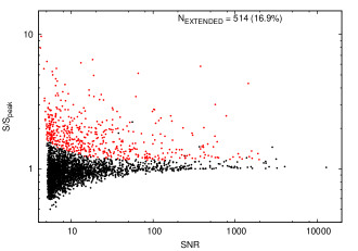
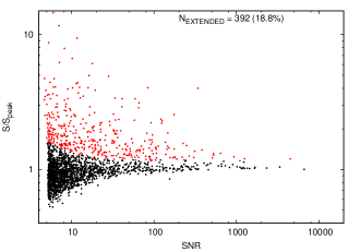
Figure 8: $S/S_{\mathrm{peak}}$ as a function of SNR for all components in CDFS (left) and ELAIS-S1 (right). The peak flux density values have been corrected for peak bias and bandwidth smearing as measured in BLOBCAT. Components which are classified as point-like/extended are shown in black/red.

A measure of the degree to which a radio source is resolved is given by the ratio of the integrated flux density, $S$, to the peak flux density, $S_{\rm peak}$:

$$\frac{S}{S_{\rm peak}}=\frac{\theta_{\rm min}\theta_{\rm max}}{B_{\rm maj}B_{\rm min}}\ ,$$ (6)

where $\theta_{\rm min}$ and $\theta_{\rm max}$ are the source fitted FWHM axes.

In Fig. 8, we plot $S/S_{\mathrm{peak}}$ as a function of SNR for CDFS in the left panel and for ELAIS-S1 in the right panel. The peak flux density has been corrected for bandwidth smearing and peak bias. The distribution of components is skewed to higher flux density ratios at higher SNR, a result of extended components. The occurrence of components with $S/S_{\mathrm{peak}}<1$ are from noise fluctuations and calibration errors. For point sources, assuming that $\sigma_{S_{\mathrm{peak}}}$ and $\sigma_{\mathrm{S}}$ are independent, $R=\ln(S/S_{\mathrm{peak}})$ has a Gaussian distribution centred on zero whose rms is given by

$$\sigma_{\mathrm{R}}=\sqrt{\left(\frac{\sigma_{\mathrm{S}}}{S}\right)^{2}+\left(\frac{\sigma_{S_{\mathrm{peak}}}}{S_{\mathrm{peak}}}\right)^{2}}\ .$$ (7)

To detect an extended source at the 2$\sigma$ level, we require $R>2\sigma_{\mathrm{R}}$ or

$$R>2\sqrt{\left(\frac{\sigma_{\mathrm{S}}}{S}\right)^{2}+\left(\frac{\sigma_{S_{\mathrm{peak}}}}{S_{\mathrm{peak}}}\right)^{2}}\ .$$ (8)

The probability of falsely classifying a point source as extended at the 2$\sigma$ level is 2.3 per cent.

We used Equation 8 to separate point-like from extended sources. $\sigma_{S_{\rm peak}}$ is taken as the sum in quadrature of the calibration error, the pixellation uncertainty (see Appendices A and B of Hales et al., 2012) and the local rms noise; the calibration error is set to $0.05~{}S_{\rm peak}$ (see Section 4.6.1) and the pixellation uncertainty to $0.01~{}S_{\rm peak}$. $\sigma_{S}$ is taken as the sum in quadrature of the calibration error and the local rms noise; the calibration error is set to $0.05~{}S$. At high SNR, where $\sigma_{\mathrm{S}}/S\approx 0.05$ and $\sigma_{\mathrm{S_{\mathrm{peak}}}}/S_{\mathrm{peak}}\approx 0.05$, $S/S_{\mathrm{peak}}$ must be greater than 1.15 for a source to be classified as extended. The number of components classified as extended is 514 (17 per cent) in CDFS and 392 (19 per cent) in ELAIS-S1.

The deconvolved angular size for extended sources is given by Hales et al. (2014a):

$$\Theta=\sqrt{\theta_{\rm min}\theta_{\rm max}-B_{\rm maj}B_{\rm min}}\ .$$ (9)

BLOBCAT does not directly measure $\theta_{\rm min}$ or $\theta_{\rm max}$. By substituting for $\theta_{\rm min}\theta_{\rm max}$ using Equation 6,

$$\Theta=\sqrt{\left(\frac{S}{S_{\mathrm{peak}}}-1\right)B_{\mathrm{maj}}B_{\mathrm{min}}}~{}\mathrm{.}$$ (10)

Following standard error propagation, the error on $\Theta$ is given by:

$$\sigma_{\Theta}=\frac{S}{S_{\rm peak}}\sqrt{\frac{B_{\rm maj}B_{\rm min}}{4(S/S_{\rm peak}-1)}\left[\left(\frac{\sigma_{S_{\rm peak}}}{S_{\rm peak}}\right)^{2}+\left(\frac{\sigma_{S}}{S}\right)^{2}\right]}\ .$$ (11)

4.4 Spectral Indices

The wide bandwidth of the ATLAS observations provides enough information to calculate the spectral indices over the mosaics. We have measured the spectral indices of components where the SNR was high enough to obtain a reliable measurement exclusively using the CABB data.

We created two separate mosaics of each field, one using the lower CABB subband data centred at $\nu_{1}=1.40\,$GHz and the other using the higher CABB subband data centred at $\nu_{2}=1.71\,$GHz, ensuring that both mosaics had the same resolution. We note that flagged frequency channels were accounted for in MIRIAD when calculating the central frequencies of the two subbands.

To measure the spectral indices of isolated components, we ran BLOBCAT on the two CABB subband mosaics using a $5\sigma$ detection limit. If a component was classified as extended in the final catalogue, we used its integrated flux density at $\nu_{1}$ and $\nu_{2}$ as measured by BLOBCAT to calculate its spectral index, otherwise we used its peak flux density. We did not measure the spectral indices of components detected below $5\sigma$ at $\nu_{1}$ or $\nu_{2}$.

We derived the spectral indices of complex components by measuring their integrated flux densities in the two CABB subband images. The integrated flux density of a complex component in each subband image was measured by summing the pixel values within its integration area (as measured in the raw BLOBCAT catalogue described in Section 4.2), and dividing by the number of pixels per beam; the advantage of this method for measuring the spectral index is that it ensures that the flux density within the exact same region of the image is compared at each frequency, which is important for components spanning several beam areas. We did not attempt to measure the spectral indices of Gaussian components which were fitted to complex components.

The error on the spectral index was taken as

$$\sigma_{\alpha}=\sqrt{\sigma_{\mathrm{\alpha,th}}^{2}+\sigma_{\mathrm{\alpha,cal}}^{2}}\ ,$$ (12)

where $\sigma_{\mathrm{\alpha,th}}$ is the uncertainty on $\alpha$ due to the thermal noise and $\sigma_{\mathrm{\alpha,cal}}$ is the calibration error on $\alpha$. The noiselike uncertainty on $\alpha$ is given by

$$\sigma_{\mathrm{\alpha,th}}=\frac{\sqrt{\left[\frac{\sigma(\nu_{1})}{S(\nu_{1})}\right]^{2}+\left[\frac{\sigma(\nu_{2})}{S(\nu_{2})}\right]^{2}}}{\beta}\ ,$$ (13)

where $S(\nu_{1})$ and $S(\nu_{2})$ are the flux densities at $\nu_{1}$ and $\nu_{2}$, $\sigma(\nu_{1})$ and $\sigma(\nu_{2})$ are the rms local noise at $\nu_{1}$ and $\nu_{2}$, and $\beta={\rm ln}(\nu_{2}/\nu_{1})$. For complex components spanning multiple beam areas, we multiplied $\sigma(\nu_{1})$ and $\sigma(\nu_{2})$ by the square root of the integration area in units of the synthesised beam.

We have identified two main types of calibration errors contributing to $\sigma_{\mathrm{\alpha,cal}}$: uncorrelated errors in the primary beam model at $\nu_{1}$ and $\nu_{2}$, and uncorrelated errors in the antenna gain calibration at $\nu_{1}$ and $\nu_{2}$. Primary beam model errors are expected to have the largest contribution close to the edges of the mosaics. As mentioned in Section 4.2, source extraction was limited to the region where the mosaicked primary beam response is above 40 per cent. The 40 per cent power level at $\nu_{2}$ corresponds to a distance from the pointing centre, $d$, of approximately 16 arcmin. In Section 4.4.1, we show that primary beam model errors cause $\alpha$ to flatten by no more than $\approx 0.1$ at $d=20$ arcmin. We conclude that, for a component located at any position within the mosaics, primary beam model errors introduce a spectral index error of at most $\approx 0.1$.

Given the very high degree of correlation ($\gtrapprox 95$ per cent) of gain calibration errors in the two CABB subbands, we have established that their contribution to $\sigma_{\mathrm{\alpha,cal}}$ is much less than 0.1. Since primary beam model errors are likely to be the dominant contribution to $\sigma_{\mathrm{\alpha,cal}}$, we set $\sigma_{\mathrm{\alpha,cal}}=0.1$.

In total, we measured spectral indices for 1756 isolated components and 163 complex components. Of the 1919 spectral index measurements, 344 have $\sigma_{\alpha}$ less than 0.2. We have included a column containing the spectral index in the final component catalogue for each field (see Table 5). The spectral index properties of the ATLAS DR3 components are discussed further in Paper II (Banfield et al., in preparation).

4.4.1 Verifying off-axis spectral index measurements

In 2010, measurements of the primary beam for the new ATCA 16 cm receivers were carried out. The radial profile of the beam was measured along eight cuts at $45^{\circ}$ intervals, at 14 regularly-spaced frequencies across the band. The shape of the beam out to the first null was found to be close to circularly symmetric across the entire frequency range. A Gaussian fit to the beam was made at each frequency out to a level of $\sim 20\%$ of the beam, using data from all angles. The product of the primary beam FWHM and the frequency was found to increase by 7 per cent between 1.3 and 1.8 GHz. This is probably due to a slight defocussing between these two frequencies.

As mentioned in Section 2.4, we used these Gaussian primary beam fits for primary beam correction. A small error in the primary beam model may introduce a bias in the measured spectral indices away from the pointing centre. We therefore tested whether there was any systematic change in the spectral index with distance from the pointing centre. We applied the primary beam correction to each pointing in CDFS and ELAIS-S1 and restored them to a common resolution. We identified sources in the raw BLOBCAT catalogue for the relevant field which were located within 20 arcmin from the pointing centre and with $\mathrm{SNR}>200$. We measured the spectral indices of these sources by comparing the pixel values at their peak positions in the two CABB subband images. The top panel of Fig. 9 shows the measured spectral index as a function of the distance from the pointing centre, combining the results from all pointings. Given the SNR cut applied, the errors on the spectral indices are less than approximately 0.1. We measured the median spectral index in five distance bins (0–4, 4–8, 8–12, 12–16 and 16–20 arcmin) and fit a second order polymonial to the median data points. The median data points are shown in Table 4. There is no statistically significant change in the spectral index with distance from the pointing centre out to 20 arcmin, which corresponds to a power point of $\approx 0.25$ at 1.71 GHz. At $d=20$ arcmin, we can be confident that errors in the primary beam model cause a flattening in the spectral index of no more than $\approx 0.1$.

To illustrate how sensitive the spectral index is to errors in the primary beam model, the bottom panel of Fig. 9 shows how the spectral index varies with distance from the pointing centre using an older primary beam model by Wieringa et al. (1992), where the beam FWHM varies as $\nu^{-1}$ between 1.3 and 1.8 GHz. In this case, there is a clear bias in the spectral index away from the pointing centre; the bias is $\approx 0.25$ at the half power point at 1.71 GHz.

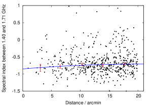
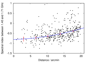
Figure 9: Spectral index between 1.40 and 1.71 GHz as a function of distance from the pointing centre for bright sources present in the CDFS and ELAIS-S1 pointings. The red points show median values in five distance bins, which are tabulated in Table 4. The blue curve shows a quadratic fit to the median data points. Top: results using Gaussian primary beam fits for the new 16 cm CABB receivers between 1.1 and 3.1 GHz. Bottom: results obtained using an older primary beam model by Wieringa et al. (1992), where the beam FWHM varies as $\nu^{-1}$ between 1.3 and 1.8 GHz.

Table 4: Relationship between spectral index and distance from the pointing centre for bright sources in individual CDFS and ELAIS-S1 pointings. The first column gives the distance range and the second column the number of sources. The third column gives the median spectral index obtained using Gaussian primary beam fits for the new 16 cm CABB receivers between 1.1 and 3.1 GHz. The numbers in brackets are median spectral indices obtained using an older primary beam model by Wieringa et al. (1992), where the beam FWHM varies as $\nu^{-1}$ between 1.3 and 1.8 GHz.

$r$	$N$	$\alpha_{\mathrm{median}}$
0–4	17	$-0.82\pm 0.11$ ($-0.79\pm 0.10$)
4–8	59	$-0.78\pm 0.05$ ($-0.72\pm 0.06$)
8–12	105	$-0.72\pm 0.04$ ($-0.65\pm 0.04$)
12–16	159	$-0.74\pm 0.04$ ($-0.53\pm 0.05$)
16–20	184	$-0.70\pm 0.04$ ($-0.38\pm 0.04$)

4.5 Frequency Coverage

The combination of multiple epochs of ATLAS observations, the wider frequency coverage of the DR3 data and the amount of flagging resulted in the effective observing frequency changing slightly across the mosaics. We used the task linmos to produce a mosaic giving the effective frequency across each field. In the final component catalogue, we have included the frequency at which the source’s flux density is measured. The frequency typically lies in the range 1.45–1.50 GHz.

We have also provided a column with the source’s flux density at 1.4 GHz. This was derived using $\alpha^{1.71}_{1.40}$ if $\sigma_{\alpha^{1.71}_{1.40}}\leq 0.2$, which is typically the case for sources with $S_{1.4}>2$ mJy. In their study of the sub-mJy radio population in the Lockman Hole, Ibar et al. (2009) found no significant change in the median value of $\alpha^{1.40}_{0.61}$ as a function of $S_{1.4}$; $\alpha^{1.40}_{0.61}$ was found to be approximately –0.6 to –0.7 down to a flux density level of $S_{1.4}\gtrsim 100\mu\mathrm{Jy}$. For ATLAS sources with $\sigma_{\alpha^{1.71}_{1.40}}>0.2$ or with no measured spectral indices, we therefore assumed that $\alpha^{1.71}_{1.40}=-0.7$ to obtain $S_{1.4}$.

4.6 Calibration accuracy checks

Figure 10: Ratio of the ATLAS to VLA flux density as a function of the VLA flux density for 112 unresolved sources in the eCDFS. The VLA flux densities were obtained from Miller et al. (2013). The dashed horizontal line indicates equal flux density values and the dashed vertical line indicates the flux density (0.15 mJy) above which the ATLAS flux densities are not considered to be affected by the Eddington bias.

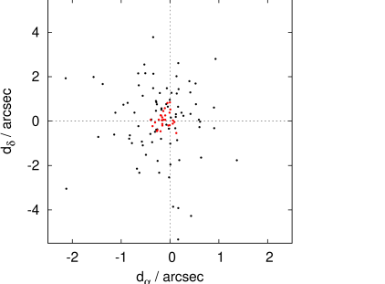
Figure 11: RA and Dec offsets between the ATLAS and VLA positions of 112 unresolved sources in the eCDFS. Sources with ATCA SNRs $\geq 20$ are shown in red and the rest of the sources in black.

Miller et al. (2013) produced an image of the Extended Chandra Deep Field South (eCDFS) with the VLA at 1.4 GHz. Their image covers an area of about a third of a square degree to a typical rms sensitivity of $7.4~{}\mu\mathrm{Jy}~{}\mathrm{bm}^{-1}$ and has a resolution of 2.8 by 1.6 arcsec. In order to assess the accuracy of the ATCA flux densities and positions presented in this paper, we matched our catalogue with the more sensitive and higher resolution catalogue by Miller et al..

4.6.1 Flux density calibration accuracy

The flux density scale for ATCA is consistent with that of Baars et al. (1973), in use at the VLA, at the 1–2 per cent level over the range 1–10 GHz (Reynolds, 1994). The VLA is more likely to resolve out part of the source flux density because of its smaller beam size. In order to minimise discrepancies between the ATCA and VLA flux densities resulting from the smaller VLA beam size, we only considered sources which were classified as point-like in both the ATCA and VLA catalogues.

Fig. 10 shows how the ATCA and VLA integrated flux densities compare for all 112 unresolved sources in common between the two surveys. There is generally excellent agreement between the flux densities. At the faint end, the ATCA flux densities tend to be systematically higher than the VLA flux densities. This is probably due, in part, to the Eddington bias (Eddington, 1913) causing the ATCA flux densities to be biased high close to the survey detection limit; the rms noise in the eCDFS region of ATLAS is $\sim 3$ times higher than that in the VLA image. The flux density boosting resulting from Eddington bias only depends on the SNR and the source count slope (Hogg & Turner, 1998). Hales et al. (2014a) used the 1.4 GHz source count fit by Hopkins et al. (2003) to evaluate the flux density boosting for a $5\sigma$ source as a function of $S_{1.4}$; the bias was estimated to be $\approx 10$ per cent at $S_{1.4}=0.1~{}\mathrm{mJy}$. This is not sufficient to explain the observed discrepancy between the ATCA and VLA flux densities at the faint end. Another potential cause of the discrepancy is missing extended flux density in the VLA image.

For sources with $S_{\rm VLA}>0.15$ mJy, the ATCA flux densities do not appear to be affected by the Eddington bias. For these 74 sources, the ATCA flux densities are, on average, consistent with the VLA flux densities at the $\approx 2$ per cent level: the mean value of $S_{\rm ATCA}/S_{\rm VLA}$ is $0.986\pm 0.013$ and the median value is $0.974\pm 0.016$.

At high SNRs, calibration errors will become the main source of uncertainty. Of the 112 ATCA-VLA sources, 29 have ATCA SNRs $\geq 20$. For these 29 sources, the standard deviation of $S_{\rm ATCA}/S_{\rm VLA}$ is 0.047. We therefore set the ATCA flux density calibration error to 5 per cent. This is a conservative estimate of the flux density calibration error since it does not account for the scatter in $S_{\rm ATCA}/S_{\rm VLA}$ introduced by errors on the VLA flux densities.

4.6.2 Positional accuracy

We have estimated the calibration errors $\sigma_{\mathrm{\alpha,cal}}$ and $\sigma_{\mathrm{\delta,cal}}$ in RA and Dec by comparing the ATCA positions with the VLA positions. Fig. 11 shows the RA offset, $d_{\alpha}$, and the Dec offset, $d_{\delta}$, for the 112 unresolved sources in common between the two surveys. Sources with ATCA SNRs $\geq 20$, for which calibration errors dominate the position uncertainties, are shown in red.

The positional uncertainties in RA and Dec resulting from phase errors can be expressed as $b~{}\Theta_{\alpha}$ and $b~{}\Theta_{\delta}$, where $b$ is a constant, and $\Theta_{\alpha/\delta}$ is the projected resolution in the RA/Dec direction. For the 29 sources with ATCA SNRs $\geq 20$, the standard deviation of $d_{\alpha}$ is 0.13 arcsec and the standard deviation of $d_{\delta}$ is 0.36 arcsec, indicating that $b\approx 0.021$.

To test for systematic errors, we calculated the mean offsets in RA and Dec. The mean value of $d_{\alpha}$ is ($-0.12\pm 0.02$) arcsec and the mean value of $d_{\delta}$ is ($0.07\pm 0.07$) arcsec. To account for the systematic offset in RA, we increased $\sigma_{\mathrm{\alpha,cal}}$ by 0.12 arcsec. In CDFS, we set $\sigma_{\mathrm{\alpha,cal}}=b~{}\Theta_{\alpha}+0.12~{}\mathrm{arcsec}=0.26~{}\mathrm{arcsec}$. Since the mean value of $d_{\delta}$ is consistent with zero at the 1$\sigma$ level, we assumed no systematic offset in Dec and set $\sigma_{\mathrm{\delta,cal}}=b~{}\Theta_{\delta}=0.33~{}\mathrm{arcsec}$.

It was not possible to carry out a similar analysis in ELAIS-S1 because no high resolution radio data were available to perform a comparison. Assuming no systematic errors in RA and Dec, and using the same value of $b$ as for CDFS, $\sigma_{\mathrm{\alpha,cal}}=b~{}\Theta_{\alpha}=0.16$ arcsec and $\sigma_{\mathrm{\delta,cal}}=b~{}\Theta_{\delta}=0.25$ arcsec.

We set the total position errors $\sigma_{\mathrm{\alpha}}$ and $\sigma_{\mathrm{\delta}}$ in RA and Dec to

$$\sigma_{\mathrm{\alpha}}=\sqrt{\sigma_{\mathrm{\alpha,cal}}^{2}+\sigma_{\mathrm{\alpha,th}}^{2}}$$ (14a)

$$\sigma_{\mathrm{\delta}}=\sqrt{\sigma_{\mathrm{\delta,cal}}^{2}+\sigma_{\mathrm{\delta,th}}^{2}}~{},$$ (14b)

where $\sigma_{\mathrm{\alpha,th}}$ and $\sigma_{\mathrm{\delta,th}}$ are the position errors in RA and Dec due to the significance of the component detection. blobcat (Hales et al. 2012) estimates $\sigma_{\mathrm{\alpha,th}}$ and $\sigma_{\mathrm{\delta,th}}$ as

$$\sigma_{\mathrm{\alpha,th}}=\frac{1}{1.4A}\Theta_{\alpha}$$ (15a)

$$\sigma_{\mathrm{\delta,th}}=\frac{1}{1.4A}\Theta_{\delta}~{},$$ (15b)

where $A$ is the SNR.

4.7 Component Catalogue

We have combined the source component catalogues for both the CDFS and ELAIS-S1 into one component source catalogue for ATLAS. Table 5 lists the first 14 components in the catalogue while the full catalogue can be obtained from the supplementary material. The columns of the component catalogue are defined as follows:

Column (1) – component number. A prefix indicates the field in which the component lies: ‘CI’ and ‘EI’ stand for Stokes $I$ component in CDFS and ELAIS-S1, respectively. Where multiple Gaussians were fitted to complex components, the component number is appended by the letter ‘C’ followed by the Gaussian number.

Column (2) – component IAU name given by ATLAS3 Jhhmmss.s-ddmmssC, where the letter ‘C’ stands for component in Stokes $I$. Norris et al, in preparation compiles the ATLAS DR3 source catalogue by combining the source components.

Columns (3) and (4) – intensity weighted centroid position: RA (J2000), $\alpha$, in hours:minutes:seconds, and Dec. (J2000), $\delta$, in degrees:minutes:seconds.

Columns (5) and (6) – intensity weighted centroid position: RA (J2000), $\alpha$, and Dec. (J2000), $\delta$, in deg.

Columns (7) and (8) – error on centroid position in RA, $\sigma_{\alpha}$, and in Dec., $\sigma_{\delta}$, in arcsec. These were derived as described in Section 4.6.2.

Column (9) – local rms noise level, $\sigma_{\rm local}$, in mJy beam^-1.

Column (10) – bandwidth smearing correction, $b$ (see Section 3.2).

Column (11) – effective frequency, $\nu_{\rm obs}$, in GHz, at which the source was measured in the mosaic (see Section 4.5).

Columns (12) and (13) – peak flux density, $S_{\rm peak}$, and associated error, $\sigma_{S_{\rm peak}}$, at $\nu_{\rm obs}$, in mJy beam^-1. $S_{\rm peak}$ has been corrected for peak bias and bandwidth smearing in BLOBCAT. $\sigma_{S_{\rm peak}}$ is derived as described in Section 4.3. $\nu_{\rm obs}$ is provided in column (20).

Columns (14) and (15) – integrated flux density, $S$, and associated error, $\sigma_{S}$, at $\nu_{\rm obs}$, in mJy. $\sigma_{S}$ is derived as described in Section 4.3. $S$ is set to $S_{\rm peak}$ and $\sigma_{S}$ to $\sigma_{S_{\rm peak}}$ for sources classified as point-like.

Columns (16) and (17) – peak flux density, $S_{\rm peak,1.4}$, and associated error, $\sigma_{S_{\rm peak,1.4}}$, at 1.4 GHz, in mJy beam^-1. $S_{\rm peak,1.4}$ was derived from $S_{\rm peak}$ as described in Section 4.5.

Columns (18) and (19) – integrated flux density, $S_{1.4}$, and associated error, $\sigma_{S_{1.4}}$, at 1.4 GHz, in mJy. $S_{1.4}$ was derived from $S$ as described in Section 4.5.

Columns (20) and (21) – deconvolved angular size, $\Theta$, and associated error, $\sigma_{\Theta}$, in arcsec, for sources classified as extended. $\Theta$ and $\sigma_{\Theta}$ are set to $-999$ for point sources.

Column (22) – component type, $t$: point-like (P) or extended (E) (see Section 4.3).

Columns (23) and (24) – spectral index between 1.40 and 1.71 GHz, $\alpha^{1.71}_{1.40}$, and associated error, $\sigma_{\alpha^{1.71}_{1.40}}$, as measured in Section 4.4. The spectral index is set to $-999$ if the SNR was too low for it to be measured.

Column (25) – field identifier.

Table 5: Catalogue entries for the first 14 components in the ATLAS $1.4\,$GHz component catalogue. The columns are defined in Section 4.7. The full catalogue can be found in the supplementary material using the same column format.

Component number	IAU Name	$\alpha$	$\delta$	$\alpha$	$\delta$	$\sigma_{\alpha}$	$\sigma_{\delta}$	$\sigma_{\rm local}$	$b$	$\nu_{\rm obs}$	$S_{\rm peak}$
				(deg)	(deg)	(arcsec)	(arcsec)	(mJy bm-1)		(GHz)	(mJy bm-1)
(1)	(2)	(3)	(4)	(5)	(6)	(7)	(8)	(9)	(10)	(11)	(12)
EI0001	ATLAS3 J002925.7-440256C	00:29:25.73	-44:02:56.6	7.357191	-44.049053	0.44	0.69	0.052	1.08	1.439	0.751
EI0002	ATLAS3 J002926.7-440016C	00:29:26.79	-44:00:16.5	7.361610	-44.004578	1.07	1.65	0.051	1.08	1.440	0.288
EI0003	ATLAS3 J002933.7-440118C	00:29:33.70	-44:01:18.4	7.390433	-44.021768	0.79	1.22	0.046	1.08	1.447	0.349
EI0004	ATLAS3 J002938.1-432946C	00:29:38.17	-43:29:46.2	7.409025	-43.496162	0.34	0.52	0.045	1.09	1.446	0.904
EI0005	ATLAS3 J002938.9-440031C	00:29:38.91	-44:00:31.2	7.412115	-44.008663	0.70	1.08	0.043	1.07	1.452	0.367
EI0006	ATLAS3 J002940.1-440308C	00:29:40.19	-44:03:08.7	7.417454	-44.052408	0.60	0.92	0.042	1.07	1.452	0.434
EI0007	ATLAS3 J002941.3-435334C	00:29:41.34	-43:53:34.0	7.422268	-43.892779	0.61	0.95	0.043	1.08	1.440	0.430
EI0008	ATLAS3 J002941.8-440714C	00:29:41.80	-44:07:14.1	7.424153	-44.120575	0.99	1.53	0.042	1.08	1.447	0.252
EI0009	ATLAS3 J002943.1-440813C	00:29:43.11	-44:08:13.3	7.429629	-44.137028	0.77	1.19	0.042	1.08	1.446	0.333
EI0010	ATLAS3 J002944.3-433629C	00:29:44.30	-43:36:29.0	7.434567	-43.608068	0.63	0.98	0.049	1.09	1.435	0.480
EI0011C1	ATLAS3 J002945.3-432148C	00:29:45.34	-43:21:48.0	7.438908	-43.363342	0.16	0.26	0.042	1.08	1.444	6.506
EI0011C2	ATLAS3 J002946.1-432148C	00:29:46.17	-43:21:48.7	7.442358	-43.363537	0.16	0.26	0.042	1.08	1.445	7.060
EI0012	ATLAS3 J002946.3-440724C	00:29:46.33	-44:07:24.0	7.443055	-44.123333	0.82	1.27	0.040	1.07	1.450	0.289
EI0013	ATLAS3 J002948.6-435618C	00:29:48.66	-43:56:18.6	7.452745	-43.938512	0.71	1.10	0.037	1.07	1.454	0.315

Table 6: continued

$\sigma_{S_{\rm peak}}$	$S$	$\sigma_{\rm S}$	$S_{\rm peak,1.4}$	$\sigma_{S_{\rm peak,1.4}}$	$S_{1.4}$	$\sigma_{S_{1.4}}$	$\Theta$	$\sigma_{\Theta}$	$t$	$\alpha^{1.71}_{1.40}$	$\sigma_{\alpha^{1.71}_{1.40}}$	Field
(mJy bm-1)	(mJy)	(mJy)	(mJy bm-1)	(mJy bm-1)	(mJy)	(mJy)	(arcsec)	(arcsec)
(13)	(14)	(15)	(16)	(17)	(18)	(19)	(20)	(21)	(22)	(23)	(24)	(25)
0.068	0.751	0.068	0.766	0.070	0.766	0.070	-999.0	-999.0	P	-0.83	1.01	ELAIS-S1
0.057	0.288	0.057	0.294	0.059	0.294	0.059	-999.0	-999.0	P	-999.00	-999.00	ELAIS-S1
0.052	0.349	0.052	0.357	0.054	0.357	0.054	-999.0	-999.0	P	-999.00	-999.00	ELAIS-S1
0.067	0.904	0.067	0.924	0.069	0.924	0.069	-999.0	-999.0	P	-2.72	0.93	ELAIS-S1
0.049	0.367	0.049	0.377	0.051	0.377	0.051	-999.0	-999.0	P	-999.00	-999.00	ELAIS-S1
0.051	0.434	0.051	0.445	0.052	0.445	0.052	-999.0	-999.0	P	-999.00	-999.00	ELAIS-S1
0.051	0.430	0.051	0.438	0.052	0.438	0.052	-999.0	-999.0	P	-999.00	-999.00	ELAIS-S1
0.047	0.252	0.047	0.258	0.048	0.258	0.048	-999.0	-999.0	P	-999.00	-999.00	ELAIS-S1
0.049	0.333	0.049	0.340	0.050	0.340	0.050	-999.0	-999.0	P	-999.00	-999.00	ELAIS-S1
0.059	0.480	0.059	0.489	0.060	0.489	0.060	-999.0	-999.0	P	-999.00	-999.00	ELAIS-S1
0.330	7.983	0.406	6.703	0.341	8.224	0.420	4.6	0.9	E	-0.96	0.15	ELAIS-S1
0.357	8.632	0.438	7.278	0.370	8.899	0.454	4.5	0.9	E	-0.96	0.15	ELAIS-S1
0.045	0.289	0.045	0.296	0.046	0.296	0.046	-999.0	-999.0	P	-999.00	-999.00	ELAIS-S1
0.043	0.315	0.043	0.323	0.044	0.323	0.044	-999.0	-999.0	P	-999.00	-999.00	ELAIS-S1

5 Conclusion

We present images and a component catalogue from a deep, wideband, radio continuum survey with ATCA. The third ATLAS data release combines observations taken between 2002 and 2010 of an area coincident with the CDFS and ELAIS-S1, two of the best-studied regions of the sky at all wavelengths. The survey covers a total area of 6.3 $\mathrm{deg}^{2}$ to a typical rms noise level of $15\,\mu$Jy beam^-1 at 1.4 GHz. Various array configurations were employed to maximise the uv coverage, resulting in a resolution of 16 by 7 arcsec in CDFS and 12 by 8 arcsec in ELAIS-S1. ATLAS is among the deepest and widest radio surveys to date and is being used as a pilot survey for EMU, which will cover the whole Southern Sky to approximately the same depth as ATLAS, at a similar resolution and frequency.

In Paper II, we present the first results from the survey, including the deep 1.4-GHz source counts. Here, we have concentrated on developing techniques for producing and analysing the radio maps to enable maximum scientific return from the survey. In particular, we have:

1. developed strategies to automatically flag data taken with the new CABB correlator between 1.3 and 1.8 GHz, and calibrate the data while accounting for frequency-dependent variations in the gains;

2. used a variety of techniques, such as multi-frequency CLEAN, self-calibration and wideband primary beam correction, to produce images with high dynamic range and fidelity;

3. run the BLOBCAT source finder on our maps while applying corrections for bandwidth smearing and peak bias to the source flux densities, resulting in a total of 5118 components above $5\sigma$ in the two fields.

4. used the wide bandwidth of our observations to measure the spectral indices across the CABB band (1.3–1.8 GHz) of $\sim 2000$ of the brightest components in the fields. Analysis of the spectral index results will be presented in Paper II.

Appendix A Observational information on ATLAS fields

Table 7: Observational information on the two ATLAS fields including observing dates, ATCA array configurations, and net integration times after calibration and flagging.

Field	Project	Date	Configuration	Integration
	ID			Time (h)
CDFS	C1035a,c,d	2002 Apr 4–7, 10, 12–13	6A	72.9
		2002 Aug 23–24, 27–29	6C	29.6
	C1241a,c,d	2004 Jan 7–8, 12	6A	23.9
		2004 Feb 3–5	6B	24.7
		2004 Jun 6, 8–12	750D	37.4
		2004 Nov 24–30	6D	50.4
		2004 Dec 28–30	1.5D	22.6
	C1241c,d	2005 Jan 7–8, 18–19, 23	750B	31.9
		2005 Apr 9–10	6A	18.5
		2005 Apr 14	1.5A	8.9
		2005 Apr 22; 2005 May 2	750A	15.0
		2005 Jun 1, 10	EW367	11.7
		2005 Jun 25–26	6B	18.1
		2005 Dec 6	6A	8.7
		2006 Mar 23–24, 27	6C	23.0
	C1967d	2009 Jun 19–21, Dec 19–31, 2010 Jan 1–3, Apr 1–6, 12, 14–18	6A	148.1
		2009 Aug 13, 19, 21–27	6D	76.6
		2009 Nov 10–18, 20–29	6B	161.0
		2010 May 1–3, 20–24, Jun 1, 5–9, 11–14, 27	6C	40.5
ELAIS-S1	C1241b,c,d	2004 Jan 9–11	6A	24.6
		2004 Jan 30, Feb 1	6B	18.6
		2004 Dec 19, 27, 2005 Jan 1–3	1.5D	40.2
		2005 Jan 9–11, 20–22	750B	50.0
		2005 Mar 25, Apr 8, 11	6A	27.2
		2005 Apr 24, 26, 30, May 1	750A	34.3
		2005 June 8, 9	EW367	18.3
		2005 June 19, 24	6B	18.5
	C1967d	2009 Dec 19–31, 2010 Jan 1–3, Apr 1–6, 12, 14–18	6A	68.6
		2009 Aug 13, 19, 21–27	6D	87.9
		2009 Nov 10–18, 20–29	6B	9.8
		2010 Apr 19	6C	10.6
		a Data presented in Norris et al. (2006).
		b Data presented in Middelberg et al. (2008).
		c Data presented in Hales et al. (2014a).
		d Data presented in this work.

Table 8: Coordinates of mosaic pointings in the two ATLAS fields.

Pointing	R.A. (J2000)	Decl. (J2000)
CDFS
1	03:28:47.33	$-$28:38:37.98
1a	03:27:18.36	$-$28:38:31.14
2	03:28:03.89	$-$28:21:46.74
3	03:28:48.48	$-$28:05:05.58
3a	03:27:18.36	$-$28:05:05.58
4	03:28:05.26	$-$27:48:14.34
5	03:28:49.61	$-$27:31:32.82
5a	03:27:18.36	$-$27:31:32.82
10	03:30:16.97	$-$27:31:40.02
11	03:29:32.83	$-$27:48:22.98
12	03:30:16.30	$-$28:05:12.42
13	03:29:31.92	$-$28:21:55.74
14	03:30:15.60	$-$28:38:44.82
15	03:31:43.87	$-$28:38:48.42
16	03:30:59.95	$-$28:22:00.78
27	03:32:27.99	$-$28:22:02.58
28	03:33:12.12	$-$28:38:48.42
29	03:34:40.39	$-$28:38:44.82
30	03:33:56.02	$-$28:22:00.78
31	03:34:39.70	$-$28:05:12.42
33	03:34:39.03	$-$27:31:40.02
41	03:32:28.00	$-$27:48:30.00
42	03:31:20.17	$-$27:48:30.00
43	03:31:54.08	$-$28:01:29.44
44	03:33:01.92	$-$28:01:29.44
45	03:33:35.83	$-$27:48:30.00
46	03:33:01.92	$-$27:35:30.56
47	03:31:54.08	$-$27:35:30.56
ELAIS-S1
1	00:32:03.55	$-$43:44:51.24
2	00:31:10.95	$-$43:27:59.64
3	00:32:05.04	$-$43:11:18.84
4	00:33:51.29	$-$43:11:24.96
5	00:32:57.67	$-$43:28:09.00
6	00:33:50.79	$-$43:44:57.36
7	00:35:38.02	$-$43:44:57.36
8	00:34:44.40	$-$43:28:11.88
9	00:35:37.51	$-$43:11:24.96
10	00:37:23.76	$-$43:11:18.84
11	00:36:31.13	$-$43:28:09.00
12	00:37:25.25	$-$43:44:51.24
13	00:36:31.13	$-$44:01:42.84
14	00:37:25.25	$-$44:18:34.44
15	00:35:38.02	$-$44:18:34.44
16	00:34:44.40	$-$44:01:42.84
17	00:32:57.67	$-$44:01:42.84
18	00:33:50.79	$-$44:18:34.44
19	00:32:03.55	$-$44:18:34.44
20	00:31:10.95	$-$44:01:42.84

References

- Afonso et al. (2007) Afonso J. et al., 2007, ASP Conf. Ser., 380, 243
- Baars et al. (1973) Baars J. W. M., Genzel R., Pauliny-Toth I. I. K., Witzel A., 1977, A&A, 61, 99
- Banerji et al. (2008) Banerji M., Abdalla F. B., Lahav O., Lin H., 2008, MNRAS, 386, 1219
- Becker, White & Helfand (1995) Becker R. H., White R. L., Helfand D. J., 1995, ApJ, 450, 559
- Bonzini et al. (2013) Bonzini M., Padovani P., Mainieri V., Kellermann K. I., Miller N., Rosati P., Tozzi P., Vattakunnel S., 2013, MNRAS, 436, 3759
- Briggs (1995) Briggs D. S., 1995, American Astronomical Society, 27, #112.02
- Bunton & Hay (2010) Bunton J. D., Hay S. G., 2010, Electromagnetics in Advanced Applications (ICEAA), p. 728
- Cohen et al. (2007) Cohen A. S., Lane W. M., Cotton W. D., Kassim N. E., Lazio T. J. W., Perley R. A., Condon J. J., Erickson W. C., 2007, AJ, 134, 1245
- Coil et al. (2011) Coil A. L. et al., 2011, ApJ, 741, 8
- Condon et al. (1998) Condon J. J., Cotton W. D., Greisen E. W., Yin Q. F., Perley R. A., Taylor G. B., Broderick J. J., 1998, AJ, 115, 1693
- Condon et al. (2003) Condon J. J., Cotton W. D., Yin Q. F., Shupe D. L., Storrie-Lombardi L. J., Helou G., Soifer B. T., Werner M. W., 2003, AJ, 125, 2411
- Condon et al. (2012) Condon J. J. et al., 2012, ApJ, 758, 23
- Cool et al. (2013) Cool R. J. et al., 2013, ApJ, 767, 118
- DeBoer et al. (2009) DeBoer D. R. et al., 2009, Institute of Electrical and Electronics Engineers Proceedings, 97, 1507
- de Vries et al. (2002) de Vries W. H., Morganti R., Röttgering H. J. A., Vermeulen R., van Breugel W., Rengelink R., Jarvis M. J., 2002, AJ, 123, 1784
- Eddington (1913) Eddington A. S., 1913, MNRAS, 73, 359
- AMI Consortium: Franzen et al. (2011) AMI Consortium: Franzen T. M. O. et al., 2011, MNRAS, 415, 2699
- Franzen et al. (2014) Franzen T. M. O. et al., 2014, MNRAS, 439, 1212
- Frater, Brooks, & Whiteoak (1992) Frater R. H., Brooks J. W., Whiteoak J. B., 1992, JEEEA, 12, 103
- Giacconi et al. (2001) Giacconi R. et al., 2001, ApJ, 551, 624
- Giavalisco et al. (2004) Giavalisco M. et al., 2004, ApJ, 600, L93
- Greisen (1983) Greisen E. W., 1983, AIPS Memo No. 27, NRAO, Charlottesville, VA
- Gruppioni et al. (1997) Gruppioni C., Zamorani G., de Ruiter H. R., Parma P., Mignoli M., Lari C., 1997, MNRAS, 286, 470
- Hales et al. (2012) Hales C. A., Murphy T., Curran J. R., Middelberg E., Gaensler B. M., Norris R. P., 2012, MNRAS, 425, 979
- Hales et al. (2014a) Hales C. A. et al., 2014, MNRAS, 441, 2555
- Hales et al. (2014b) Hales C. A., Norris R. P., Gaensler B. M., Middelberg E., 2014, MNRAS, 440, 3113
- Hancock et al. (2012) Hancock P. J., Murphy T., Gaensler B. M., Hopkins A., Curran J. R., 2012, ascl.soft, 12009
- Hodge et al. (2011) Hodge J. A., Becker R. H., White R. L., Richards G. T., Zeimann G. R., 2011, AJ, 142, 3
- Hogg & Turner (1998) Hogg D. W., Turner E. L., 1998, PASP, 110, 727
- Hopkins et al. (2003) Hopkins A. M., Afonso J., Chan B., Cram L. E., Georgakakis A., Mobasher B., 2003, AJ, 125, 465
- Hurley-Walker et al. (2014) Hurley-Walker N. et al., 2014, Publications of the Astronomical Society of Australia, 31, e045
- Huynh et al. (2012) Huynh M. T., Hopkins A. M., Lenc E., Mao M. Y., Middelberg E., Norris R. P., Randall K. E., 2012, MNRAS, 426, 2342
- Huynh et al. (2012) Huynh M. T., Hopkins A., Norris R., Hancock P., Murphy T., Jurek R., Whiting M., 2012, Publications of the Astronomical Society of Australia, 29, 229
- Ibar et al. (2009) Ibar E., Ivison R. J., Biggs A. D., Lal D. V., Best P. N., Green D. A., 2009, MNRAS, 397, 281
- Intema (2014) Intema H. T., 2014, arXiv:1402.4889
- Jarvis et al. (2013) Jarvis M. J. et al., MNRAS, 2013, 428, 1281
- Johnston et al. (2007) Johnston S. et al., 2007, Publications of the Astronomical Society of Australia, 24, 174
- Johnston et al. (2008) Johnston S. et al., 2008, ExA, 22, 151
- Koekemoer, Mobasher & Norris (2003) Koekemoer A. M., Mobasher B., Norris R. P., 2003, NewAR, 47, 391
- Lenc et al. (2009) Lenc E. et al., 2009, Proceedings of Panoramic Radio Astronomy, 28
- Lonsdale et al. (2003) Lonsdale C. J. et al., 2003, PASP, 115, 897
- Mao et al. (2012) Mao M. Y. et al., 2012, MNRAS, 426, 3334
- Mauch et al. (2003) Mauch T., Murphy T., Buttery H. J., Curran J., Hunstead R. W., Piestrzynski B., Robertson J. G., Sadler E. M., 2003, MNRAS, 342, 1117
- Mauduit et al. (2012) Mauduit J. C. et al., 2012, PASP, 124, 1135
- Middelberg (2006) Middelberg E., 2006, Publications of the Astronomical Society of Australia, 23, 64
- Middelberg et al. (2008) Middelberg E. et al., 2008, AJ, 135, 1276
- Miller et al. (2013) Miller N. A. et al., 2013, ApJS, 205, 13
- Morganti et al. (2004) Morganti R., Garrett M. A., Chapman S., Baan W., Helou G., Soifer T., 2004, A&A, 424, 371
- Norris et al. (2006) Norris R. P. et al., 2006, AJ, 132, 2409
- Norris et al. (2011) Norris R. P. et al., 2011, Publications of the Astronomical Society of Australia, 28, 215
- Oliver et al. (2000) Oliver S. et al., 2000, MNRAS, 316, 749
- Oliver et al. (2012) Oliver S. J. et al., 2012, MNRAS, 424, 1614
- Owen & Morrison (2008) Owen F. N., Morrison G. E., 2008, AJ, 136, 1889
- Prandoni et al. (2000) Prandoni I., Gregorini L., Parma P., de Ruiter H. R., Vettolani G., Wieringa M. H., Ekers R. D., 2000, A&AS, 146, 41
- Randall et al. (2012) Randall K. E., Hopkins A. M., Norris R. P., Zinn P.-C., Middelberg E., Mao M. Y., Sharp R. G., 2012, MNRAS, 421, 1644
- Rau & Cornwell (2011) Rau U., Cornwell T. J., 2011, A&A, 532, A71
- Rees (1990) Rees N., 1990, MNRAS, 244, 233
- Reynolds (1994) Reynolds J. E., 1994, ATNF internal memo AT/39.3/040
- Röttgering et al. (2010) Röttgering H. et al., 2010, www.astron.nl/radio-observatory/apertif-eoi-abstracts-and-contact-information
- Sault, Teuben, & Wright (1995) Sault R. J., Teuben P. J., Wright M. C. H., 1995, ASP Conf. Ser., 77, 433
- Sault, Staveley-Smith & Brouw (1996) Sault R. J., Staveley-Smith L., Brouw W. N., 1996, A&AS, 120, 375
- Sault & Conway (1999) Sault R. J., Conway J. E., 1999, ASP Conf. Ser., 180, 419
- Schinnerer et al. (2007) Schinnerer E. et al., 2007, ApJS, 172, 46
- Seymour et al. (2008) Seymour N. et al., 2008, MNRAS, 386, 1695
- Shepherd (1997) Shepherd M. C., 1997, ASP Conf. Ser., 125, 77
- Sirothia et al. (2012) Sirothia S. K., Kantharia N. G., Ishwara-Chandra C. H., Gopal-Krishna, 2012, http://tgss.ncra.tifr.res.in/, accessed: 2013-11-15
- Smolčić et al. (2008) Smolčić V. et al., 2008, ApJS, 177, 14
- Spitler et al. (2012) Spitler L. R. et al., 2012, ApJ, 748, L21
- Wayth et al. (2015) Wayth R. B. et al., 2015, Publications of the Astronomical Society of Australia, 32, e025
- Wieringa et al. (1992) Wieringa M. H., 1992, Experimental Astronomy, 2, 203
- Wieringa & Kesteven (1992) Wieringa M. H., Kesteven M. J., 1992, ATNF internal memo AT/39.3/024
- Wilson et al. (2011) Wilson W. E. et al., 2011, MNRAS, 416, 832
- Xue et al. (2011) Xue Y. Q. et al., 2011, ApJS, 195, 10
- Zinn et al. (2012) Zinn P.-C., Middelberg E., Norris R. P., Hales C. A., Mao M. Y., Randall K. E., 2012, A&A, 544, A38