Local and global aspects of the linear MRI in accretion disks

Abstract

We revisit the linear MRI in a cylindrical model of an accretion disk and uncover a number of attractive results overlooked in previous treatments. In particular, we elucidate the connection between local axisymmetric modes and global modes, and show that a local channel flow corresponds to the evanescent part of a global mode. In addition, we find that the global problem reproduces the local dispersion relation without approximation, a result that helps explain the success the local analysis enjoys in predicting global growth rates. MRI channel flows are nonlinear solutions to the governing equations in the local shearing box. However, only a small subset of MRI modes share the same property in global disk models, providing further evidence that the prominence of channels in local boxes is artificial. Finally, we verify our results via direct numerical simulations with the Godunov code RAMSES.

1 Introduction

The magnetorotational instability (MRI) remains the principal mechanism facilitating turbulence, and consequently mass accretion, in astrophysical disks. Since the seminal paper of Balbus and Hawley (1991, hereafter BH91), numerical simulations of MRI turbulence have become increasingly sophisticated and comprehensive; now computations in global disk geometry are relatively common (e.g. Penna et al. 2010, Hawley et al. 2013, Parkin & Bicknell 2013) as is the inclusion of a panoply of physical effects (e.g. Jiang et al. 2013, Hirose et al. 2014, Lesur et al. 2014, Bai 2014). Despite this increase in complexity, BH91’s local and incompressible linear theory continues to guide the interpretation of the simulation results with surprising success (Flock et al. 2010, Hawley et al. 2011, Okuzumi & Hirose 2011).

When it first appeared, however, the analysis of BH91 provoked a debate concerning the local approach’s validity when describing phenomena in the global geometry of an accretion disk. The emphasis of the debate focussed, in particular, on the small imaginary part exhibited by the MRI growth rates (neglected in the local analysis) as well as the boundary conditions’ impact on the magnitude of the growth (also neglected; Knobloch 1992, Dubrulle & Knobloch 1993). Ultimately, these concerns were shown to be somewhat exaggerated. Analyses in cylindrical models, vertically stratified boxes, and general geometries indicated that the stability criterion was unaltered and the local growth rates good approximations in most instances (Kumar et al. 1994, Papaloizou & Szuszkiewicz 1994, Gammie & Balbus 1994, Curry et al. 1994, Curry & Pudritz 1995, Terquem & Papaloizou 1996, Ogilvie 1998).

One issue that remains undeveloped is the question of how the BH91 local modes actually manifest in global disks. In other words: how do the local and global formalisms join up? This is especially important for the MRI channel modes, the fastest growing, because in the local analysis they exhibit no radial variation at all. This implies that their radial variation is in fact global. What might their radial structure be — and does it matter? A second issue, also unexplored, is the nature of the modes that participate in simulations of global MHD turbulence. Simulated modes are never strictly local because of resolution constraints. We may ask how well such modes can be understood via the local approach. We may also want to construct a taxonomy of global modes and determine how they control the turbulence and other global aspects of the disk evolution (zonal flows, winds, magnetic flux diffusion, etc).

In this paper we make explicit the connection between the local and global MRI, by revisiting the incompressible axisymmetric cylindrical disk models employed by Dubrulle & Knobloch (1993), Coleman et al. (1994) and Curry et al. (1994). In so doing we uncover a number of attractive and overlooked results. First, we show that the global problem reproduces the (discretised) local dispersion relation without approximation. The boundary conditions only determine the discretisation, they do not generally influence the shape of the dispersion relation. Second, global MRI modes extend over a limited range of disk radii before decaying in an outer evanescent region in which the differential rotation is too weak. We make clear that local channel modes can be identified with these evanescent portions, while local radially varying modes can be identified with parts of the same modes at smaller radii. Third, convenient analytic approximations to the global growth rates are available via a matched WKBJ procedure. Fourth, in general, global MRI modes do not possess the nonlinear property of familiar local channel flows (Goodman & Xu 1994). Only modes localised to the inner edge of the disk remain acceptable solutions to the full equations when possessing nonlinear amplitudes. These results are verified numerically with a small set of simulations using the Godunov code, RAMSES (Teyssier 2002, Fromang et al. 2006). Finally, we discuss the issues and questions they raise, and future work that could begin to address them.

2 Linear stability analysis

Within this paper we consider an annular slice through the midplane of the disk. The slice’s vertical thickness is taken to be much less than the disk’s vertical scale height. The background vertical structure is hence neglected, and the model is quasi-global: ‘local’ in the vertical and ‘global’ in the radial. For convenience we also dispense with the disk’s radial structure and treat the ionised fluid as incompressible. The resulting formalism remains mathematically tractable while retaining important global effects (boundary conditions and curvature).

The first linear calculations in this set-up were undertaken by Velikhov (1959) and Chandrasekhar (1961), but it was not until the 1990s that accretion disks were explicitly modelled in this way (Knobloch 1992, Dubrulle & Knobloch 1993, Kumar et al. 1994, Curry et al. 1994), the latter work generally confirming the local theory of BH91. More recently, Kersalé et al. (2004) generalised the set-up to permit a radial flow of material through the inner boundary; and, while the classical MRI is recovered, spurious ‘wall modes’ are generated by the inner boundary condition. These modes control to some extent the ensuing nonlinear dynamics (Kersalé et al. 2006). Finally, we note the work of Rosin & Mestel (2012) which included the Braginskii stress, and hence could describe the onset of instability in the weakly collisional plasma of the Galactic disk.

In this section we first exhibit the main equations and repeat the classical local axisymmetric stability analysis for reference. Next the linearised equations in cylindrical geometry are reduced to a single second-order Sturm-Liouville equation, through which we display the similarities with the local problem. Numerical and analytic solutions are then derived.

2.1 Governing equations

We work with the equations of ideal incompressible MHD,

$$\partial_{t}\mathbf{u}+\mathbf{u}\cdot\nabla\mathbf{u} =-\nabla\Phi-\frac{1}{\rho}\nabla P_{t}+\frac{1}{4\pi\rho}\mathbf{B}\cdot\nabla\mathbf{B},$$ (1)

$$\partial_{t}\mathbf{B}+\mathbf{u}\cdot\nabla\mathbf{B} =\mathbf{B}\cdot\nabla\mathbf{u},$$ (2)

$$\nabla\cdot\mathbf{u} =0$$ (3)

$$\nabla\cdot\mathbf{B} =0.$$ (4)

Here velocity and magnetic field are denoted by $\mathbf{u}$ and $\mathbf{B}$ respectively, $\rho$ is the constant density, $\Phi$ is the gravitational potential of the central object, and $P_{t}$ is the combined gas and magnetic pressure. The accretion disk is a circular annulus, with gas inhabiting cylindrical radii between $r=r_{0}$ and $r=r_{1}$ with $r_{0}\ll r_{1}$. The vertical extent of the domain we set to positive and negative infinity. This setup describes motions that possess short vertical lengthscales (shorter than the scale height) and up to long radial lengthscales ($\gtrsim r_{0}$).

2.1.1 Equilibrium

The governing equations admit the steady equilibrium solution:

$$\mathbf{u}=r\Omega(r)\,\mathbf{e}_{\phi},\quad\mathbf{B}=B_{0}\,\mathbf{e}_{z},\quad P_{t}=P_{t}(r),$$ (5)

The rotation frequency is a power law,

$$\Omega=\Omega_{0}\left(\frac{r}{r_{0}}\right)^{-q}.$$

If $q=3/2$ the disk is Keplerian and the background pressure is constant (no pressure gradient is required for radial force balance). When $q\neq 3/2$ the pressure gradient is non-zero, but its details are not important in what follows (see Curry et al. 1994 for further specifics).

2.1.2 Perturbations

The equilibrium is disturbed by axisymmetric modes of the type $\propto F(r)e^{\text{i}k_{z}z+st}$, where $F$ is an $r$-dependent perturbation amplitude, $k_{z}$ is the (real) vertical wavenumber, and $s$ is the (potentially complex) growth rate. The assumption of vertical locality means that $k_{z}r_{0}\gg 1$.

The ensuing linearised equations are

$$su_{r}^{\prime}-2\Omega u_{\phi}^{\prime} =-\partial_{r}h^{\prime}+ik_{z}v_{A}^{2}b_{r}^{\prime},$$ (6)

$$su_{\phi}^{\prime}+(2-q)\Omega u_{r}^{\prime} =ik_{z}v_{A}^{2}b_{\phi}^{\prime},$$ (7)

$$su_{z}^{\prime} =-ik_{z}h^{\prime}+ik_{z}v_{A}^{2}b_{z}^{\prime},$$ (8)

$$sb_{r}^{\prime} =ik_{z}u_{r}^{\prime},$$ (9)

$$sb_{\phi}^{\prime} =ik_{z}u_{\phi}^{\prime}-q\Omega b_{r}^{\prime},$$ (10)

$$sb_{z}^{\prime} =ik_{z}u_{z}^{\prime},$$ (11)

$$(1/r)\partial_{r}(ru_{r}^{\prime})+ik_{z}u_{z}^{\prime} =0.$$ (12)

Here a prime indicates the perturbation, while $\mathbf{b}^{\prime}=B_{0}\mathbf{B}^{\prime}$ and is hence dimensionless. The Alfven speed is defined by $v_{A}^{2}=B_{0}^{2}/(4\pi\rho)$ and the enthalpy by $h^{\prime}=P_{t}^{\prime}/\rho$. Note that these perturbations automatically satisfy the solenoidal condition on $\mathbf{b}^{\prime}$.

To complete the problem we must supply two boundary conditions, applied to the radial velocity $u_{r}^{\prime}$. The boundaries can be treated as hard walls or as stress free (Dubrulle & Knobloch 1993), in which case either $u_{r}^{\prime}$ or $\partial_{r}u_{r}^{\prime}$ is zero at $r=r_{0}$ and $r=r_{1}$, or they may be treated as free surfaces (Curry et al. 1994), in which case a linear combination of $u_{r}^{\prime}$ and $\partial_{r}u_{r}^{\prime}$ is zero. As we will see later, it is not terribly important which we choose, only that the conditions are homogeneous.

Note that the Alfven frequency $k_{z}v_{A}$ associated with each mode is constant throughout the disk. In contrast, the orbital frequency $\Omega(r)$ decreases with radius. Consequently, at sufficiently large radius magnetic tension dominates and the conditions for MRI become unfavourable. We expect a growing MRI mode of given $k_{z}$ to avoid such radii and instead emerge closer to the central body. If, however, the background magnetic field decays with radius faster than $\Omega$, this need not be the case.

2.2 Local axisymmetric dispersion relation

In order to examine local modes, we choose a point $r_{*}$ and examine the behaviour of the gas in its immediate vicinity. For axisymmetric disturbances the orbital frequency $\Omega$ can be regarded as constant in Eqs (6)-(12), and if their radial variation is small-scale then the cylindrical term in Eq. (12) may be dropped. This permits us to decompose the disturbances in Fourier modes $\propto\text{e}^{\text{i}k_{x}r}$, and the local MRI dispersion relation for such modes is straightforward to derive:

$$s^{4}+[2k_{z}^{2}v_{A}^{2}+2(2-q)\epsilon^{2}\Omega_{*}^{2}]s^{2}+k_{z}^{2}v_{A}^{2}\left(k_{z}^{2}v_{A}^{2}-2q\epsilon^{2}\Omega_{*}^{2}\right)=0.$$ (13)

Here $\Omega_{*}=\Omega(r_{*})$, the rotation rate at the radius in which we’re interested, and

$$\epsilon=\frac{1}{(1+k_{x}^{2}/k_{z}^{2})^{1/2}}.$$ (14)

In Eq. (13) the radial wavenumber $k_{x}$ appears solely in $\epsilon$ and then only in the ratio $k_{x}/k_{z}$. Note also that instances of $\epsilon$ occur exclusively as factors of $\Omega_{*}$. The familiar channel flows are obtained when $k_{x}/k_{z}\to 0$, with the modes exhibiting little (to no) relative radial variation. In this case, $\epsilon\to 1$ and the fastest growth rate is achieved, $q\Omega_{*}/2$. Because $\epsilon\Omega_{*}$ sets the timescale of the growth rate, modes with non-zero $k_{x}$ grow slower, as they possess $\epsilon<1$. We call radially varying modes ‘radial modes’ to distinguish them from channel modes.

The local dispersion relation (13) exhibits an interesting connection between radial variation, on one hand, and radial location, on the other. By varying $k_{x}$ (and keeping $k_{z}$ fixed) we can ‘rescale’ the MRI timescale $\epsilon\Omega_{*}$, because the factor $\epsilon$ depends on $k_{x}$. A striking consequence is that a radial mode of a given $\epsilon$ located at one radius $r_{i}$, associated with an orbital frequency of $\Omega(r_{i})=\Omega_{*}$, possesses the same growth rate as a channel mode located at a different larger radius $r_{o}>r_{i}$, associated with an orbital frequency of $\Omega(r_{o})=\epsilon\Omega_{*}$. As a consequence, we can ‘map’ modes of different $k_{x}$, but different radial locations, onto one another.

Physically, one can understand the radial modes by returning to the classical cartoon of the MRI mechanism (for e.g. BH91). The upper panel of Fig. 1 illustrates a channel mode, with the blue circles representing fluid blobs and the black lines indicating the magnetic field (initially vertical). Vertically varying radial perturbations lead to the periodic stretching of the magnetic field and, consequently, to angular momentum exchange between the tethered blobs. The instability proceeds from the counterstreaming flows that ensue.

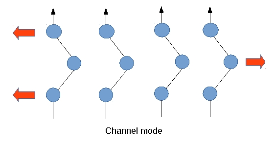
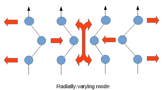
Figure 1: Simple illustrations of a channel mode (upper panel) and a radial mode (lower panel). Blue circles represent fluid blobs, the black arrows indicate the initially vertical magnetic field. Red arrows show the direction of the fluid motion.

However, if the mode possesses radial structure there will exist nodes in radius where the streams converge and diverge, illustrated in the lower panel of Fig. 1. At these radii the mode exhibits vertical deflection and pressure perturbations which are not present in pure channel flow. Needless to say, the development of vertical circulations impedes the instability mechanism exemplified in pure channel flow. During their vertical excursions fluid blobs stop extracting free energy because they are no longer exchanging angular momentum effectively.

2.3 Global eigenvalue problem

We now return to the linearised global equations (6)-(12) which can be reworked into a single second-order equation for the variable $U=r^{1/2}u_{r}^{\prime}$. Rescaling space by $r_{0}$ we find

$$\frac{d^{2}U}{dr^{2}}-\left(\frac{3}{4r^{2}}+k_{z}^{2}\right)U=-\frac{k_{z}^{2}}{r^{2q}}\varepsilon^{-2}\,U,$$ (15)

which should be solved on the domain $r\in[1,\,r_{1}/r_{0}]$. Here the various parameters appearing in the problem, in addition to the unknown growth rate $s$, have been packaged into the convenient quantity $\varepsilon$ defined via

$$\varepsilon^{-2}=2\Omega_{0}^{2}\,\frac{(q-2)s^{2}+qk_{z}^{2}v_{A}^{2}}{(s^{2}+k^{2}_{z}v_{A}^{2})^{2}}.$$ (16)

In the above, $\Omega_{0}=\Omega(r_{0})$, the rotation rate at the inner boundary.

With homogeneous boundary conditions (such as impenetrable walls or a free surface), Eq. (15) is in Sturm-Liouville form. The weight function is $-k_{z}^{2}\,r^{-2q}$ and the eigenvalue is $\varepsilon^{-2}$. Because the problem is Sturm-Liouville, we are assured of a discrete set of real eigenvalues $\varepsilon_{n}^{-2}$ which we order so that $\varepsilon_{0}>\varepsilon_{1}>\varepsilon_{2}>\dots$. Once these are computed the associated growth rates can be obtained. Hence the problem is broken down into two steps: first calculate $U$ and $\varepsilon$ from (15), then calculate the growth rate $s$ from (16). Note that the eigenfunction structure $U$ depends only on $k_{z}$; it is oblivious to the magnetic field strength $v_{A}$ unless it appears in the boundary conditions.

2.3.1 Global dispersion relation

Equation (16), which defines the eigenvalue $\varepsilon$, can be reworked into

$$s^{4}+[2k^{2}_{z}v_{A}^{2}+2(2-q)\varepsilon_{n}^{2}\Omega^{2}_{0}]s^{2}+k^{2}_{z}v_{A}^{2}\left(k^{2}_{z}v_{A}^{2}-2q\varepsilon_{n}^{2}\Omega_{0}^{2}\right)=0,$$ (17)

which is almost identical to Eq. (13)! Remarkably, the axisymmetric global problem yields a variant of the local axisymmetric dispersion relation. The basic structure of the local problem is retained independently of the global specifics: curvature and boundary conditions.

There are two differences. Instead of the function $\epsilon$, which depends smoothly on the continuous radial wavenumber $k_{x}$, the global problem possesses the discrete function $\varepsilon_{n}$ which depends on the radial quantum number $n$. Unlike the local problem, we do not know how $\varepsilon_{n}$ depends on $n$ a priori; this information must be extracted from the differential equation (15) and depends on $k_{z}$, $q$, and the boundary conditions. However, it is easy to show that $\varepsilon_{n}<1$ (see Appendix A). Hence we order the eigenvalues as $1>\varepsilon_{0}>\varepsilon_{1}>\varepsilon_{2}>\dots>0$. The second difference is that $\Omega$ is set to $\Omega_{0}$, the orbital frequency at the inner radius of the disk. This fixes the minimum timescale over which appreciable growth can happen.

It should be emphasised that, in contrast to the claims of previous authors, the only role the boundary conditions play is to help set the discretisation of the dispersion relation (17). It does not alter the shape of the relation itself. That fundamental shape is determined by the local physics, as first explained in BH91. Moreover, as we show later, the larger $r_{0}k_{z}$ the more closely spaced the $\varepsilon_{n}$ and hence the less important the discretisation.

2.3.2 Stability criterion

Next we rearrange Eq. (15) so that it resembles a Schrödinger equation,

$$\frac{d^{2}U}{dr^{2}}+k_{z}^{2}\,f(r,\varepsilon)\,U=0,$$ (18)

where

$$f(r,\varepsilon)=\frac{1}{r^{2q}}\varepsilon^{-2}-\frac{3}{4r^{2}k_{z}^{2}}-1.$$ (19)

The problem now resembles that of a particle in a potential well, with the potential proportional to $f$. It is easy to show that $f$ has an extremum at

$$r=\left(\tfrac{4}{3}qk^{2}/\varepsilon^{2}\right)^{1/[2(q-1)]}.$$ (20)

In order for there to be trapped waves, i.e. normal modes, the extremum must lie inside the disk. For simplicity we let its outer boundary go to infinity, then this condition, combined with (17), gives us a general instability criterion in terms of the vertical field

$$M_{A}>\frac{1}{q}\sqrt{\frac{3}{8}},$$ (21)

where $M_{A}$ is the Alfvénic Mach number of the background state, defined to be equal to $\Omega_{0}r_{0}/v_{A}$. The criterion (21) gives an upper bound on the magnetic field threading the disk. Because in most contexts the field is assumed to be subthermal and the disk assumed thin, we have $M_{A}\gg 1$ and the criterion is automatically satisfied. A far more restrictive condition on the magnetic field issues from the disk’s vertical thickness (see BH91 and Gammie & Balbus 1994).

2.3.3 Turning points and global and local modes

At sufficiently large $r$ the function $f$ will be dominated by the last term in Eq. (19). In this region $U\sim\text{e}^{-k_{z}r}$ and the mode is evanescent. Physically this makes sense: sufficiently far out in the disk the differential rotation is too weak to compete with magnetic tension and the MRI mechanism is suppressed. Active MRI modes will shun such a region and instead localise at smaller radii where the conditions for instability are more favourable. In Fig. 2 we present a representative eigenfunction illustrating this morphology.

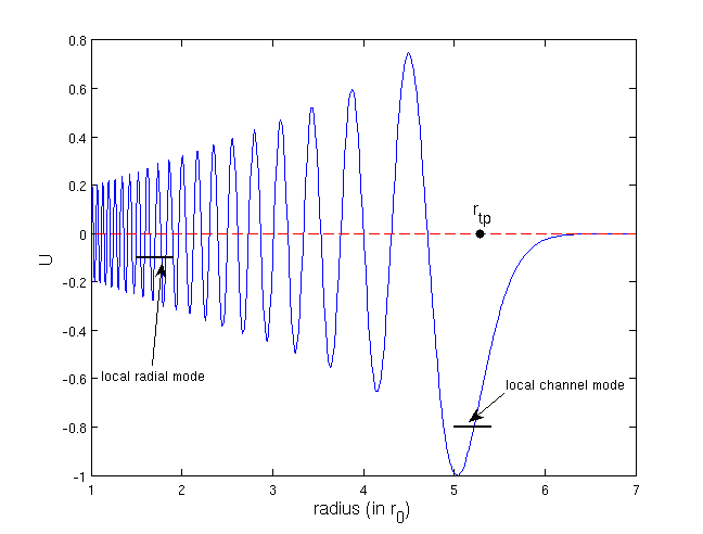
Figure 2: A higher order global eigenfunction of (15). The turning point $r_{\text{tp}}$ is indicated as are regions of the global mode that we identify with local channel and radial modes. Note also the monotonic decrease in the local radial wavenumber $k_{r}$ with radius.

The boundary between the evanescent region and the ‘MRI region’ is given by the turning point of Eq. (18), i.e. the radius at which $f=0$, denoted by $r_{\text{tp}}$. For general $q$ and $k_{z}$ this must be determined numerically. However, in the plausible limit of $k_{z}$ large,

$$r_{\text{tp}}\approx\varepsilon^{-1/q}.$$ (22)

In fact, this radius corresponds to an orbital frequency of $\Omega=\varepsilon\Omega_{0}$.

Combining this last piece of information with the local and global dispersion relations reveals an interesting correspondence. A global mode, associated with a given $\varepsilon_{n}$, shares the same dispersion relation (17) as that of a local channel mode situated at the global mode’s turning point (13). This is because the local orbital frequency $\Omega_{*}$ at this point is precisely $\varepsilon_{n}\Omega_{0}$. Consequently, we are invited to identify a local channel mode as the small section of a much larger global mode — the section near evanescence. Indeed, we may define a (radius dependent) radial wavenumber via $k_{r}\approx k_{z}\,f^{1/2}$, and at the turning point $k_{r}=f^{1/2}=0$, by definition, which is in accord with the channel mode’s lack of any radial structure.

Meanwhile, what of local radial modes? First, consider a radial mode located at $r\approx r_{0}$, i.e. very near the inner boundary, and possessing a $k_{x}$ so that $\epsilon\approx\varepsilon_{n}$, for the same $n$ as above. This particular radial mode now shares the same dispersion relation as the previous channel mode, and hence the same dispersion relation as the global mode, Eq. (17). Hence we may also identify this local radial mode as part of the same parent global mode — but the part of that mode near the inner boundary. Moreover, we can do exactly the same with other radial modes of smaller $k_{x}$. But for each different $k_{x}$ we must change the local mode’s radial location so that the timescale $\epsilon\Omega$ is kept constant.

This explains the connection between radial variation and radial location that appeared in the local dispersion relation of Section 2.2. This connection arises because a global mode of given $n$ is constituted from a set of local modes of differing $k_{x}$, each at a different radial location. In Fig. 2 this idea is sketched out.

It is worth stressing that the growth rate of the global mode is limited by the local physics at the mode’s periphery, at $r=r_{\text{tp}}$. Though the mode extends over regions where the local growth rate can be faster, the mode can only grow as fast as its outer ‘edge’. Put another way: the structure, as a whole, can only grow as fast as its slowest component. This helps remove some of the ambiguity when attributing local growth rates to global simulations. It is clear that at any given radius, growth is controlled by the mode whose turning point falls at that radius. No other mode that extends to this location can grow faster (faster growers are localised to radii closer in). Moreover, as we see from Figs 2 and 3, modes’ amplitudes are maximal near $r=r_{\text{tp}}$. Indeed, numerical simulations verify this. At any given radius, growth occurs at the rate of the local channel mode (Hawley 2001), which of course is also the rate of the global mode whose turning point $r_{\text{tp}}$ falls there.

2.4 Global solutions

2.4.1 Numerical solutions

Having sketched out the background details, we present in this subsection a few numerical solutions to (15) subject to the hard wall boundary conditions, $U=0$ at $r=1,\,r_{1}/r_{0}$. Our domain is set to be $r\in[1,10]$. The only parameter that appears explicitly in (15) is the vertical wavenumber $k_{z}$. We let it equal 10 for our main results. The numerical technique we use is a pseudo-spectral Chebyshev method (Boyd 2002), which approximates the differential equation by a matrix. Its eigenvalues may be obtained by the QZ algorithm (Golub & van Loan 1996). The boundary conditions are encoded in the matrix via boundary bordering.

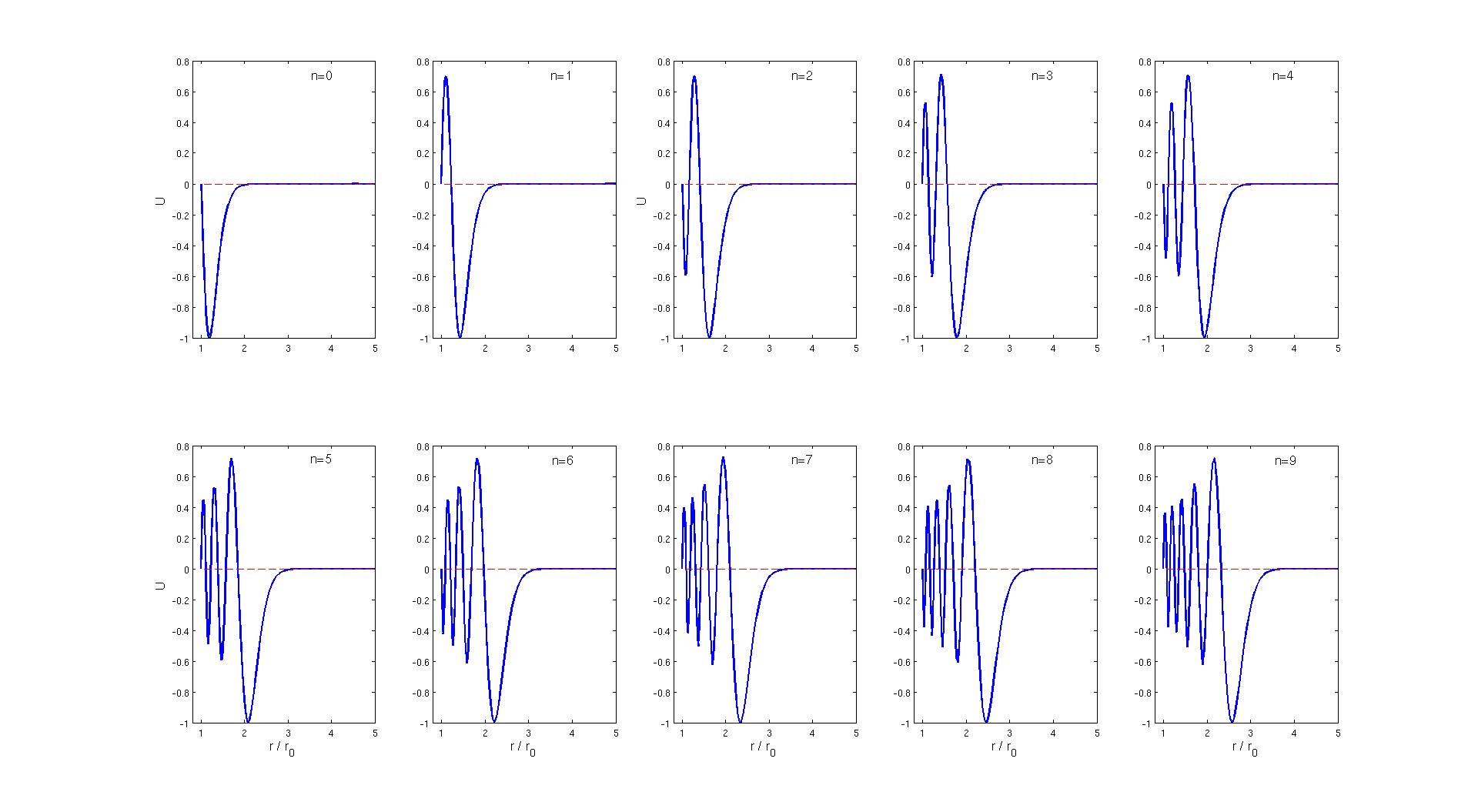
Figure 3: The first ten MRI eigenfunctions when $k_{z}=10$. In each case, the modes are oscillatory within the region $1<r<r_{\text{tp}}$ and clearly evanescent outside these. Real parts are plotted; the imaginary parts are zero.

In Fig. 3 appear the first ten eigenfunctions for $k_{z}=10$. The associated $\varepsilon_{n}$ for the first four are

$$\{0.6413,\,0.4976,\,0.4169,\,0.3628\},$$

with corresponding turning points $r_{\text{tp}}$

$$\{1.345,\,1.593,\,1.792,\,1.966\},$$

where the mode transitions to an evanescent wave. As anticipated, larger $n$ correspond to modes that extend over more of the domain.

In order to compute explicit growth rates we need to specify the strength of the vertical magnetic field, this can be measured in terms of either the dimensionless combination $v_{A}(k_{z}/\Omega)$ or the Alfvénic Mach number $M_{A}$. Selecting the first option, we plot in Fig. 4 the growth rates of the first four modes as functions of $v_{A}$ and fixed $k_{z}=10$. These are just four copies of the standard local MRI relation. The different curves correspond, not to differences in the modes’ vertical structure — this is held fixed — but to different radial structures. The greater the radial quantum number $n$ the more radial structure, but most importantly the greater $r_{\text{tp}}$ and hence the slower the dynamical timescale. This explains why higher $n$ modes grow slower. It should be appreciated that the fastest growing mode need not determine the evolution of the disk globally. The fastest growing modes are localised at small radius. Larger radii will be driven by the slower modes that extend to them.

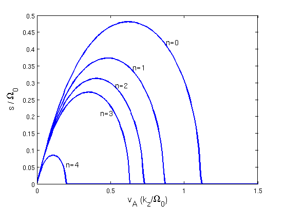
Figure 4: MRI growth rates for five different radial quantum numbers and when $k_{z}=10$ but $v_{A}$, the strength of the background magnetic field, varies. Note that $v_{A}$ has been scaled using a fixed $k_{z}$; this is so the classical MRI dispersion curves are easier to see.

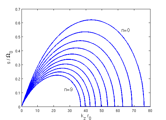
Figure 5: MRI growth rates for the first 10 radial quantum number $n$ when $v_{A}$ is fixed and $k_{z}$ is varied. We have set $M_{A}=r_{0}\Omega_{0}/v_{A}=50$.

Lastly, we fix $v_{A}$ and see how the growth rates vary as a function of $k_{z}$. In Fig. 5 we plot $s$ as a function of $k_{z}$, different $n$, and for a weak field fixed by $M_{A}=50$. These curves are similar but not exactly those of the standard MRI, seen in Fig. 4. That is, we cannot simply rescale $k_{z}r_{0}$ by $k_{z}v_{A}/\Omega_{0}$ and recover the same relation. This is because $\varepsilon_{n}=\varepsilon_{n}(k_{z})$.

2.4.2 Special solutions

For certain special cases, Eq. (15) can be solved exactly. When the disk exhibits a rotation profile of $q=1$, roughly similar to the Galaxy, we find that

$$U=r^{1/2}K_{\nu}(k_{z}r),\qquad\text{with}\qquad\nu=\sqrt{1-k_{z}^{2}/\varepsilon^{2}},$$ (23)

and where $K_{\nu}(x)$ is the modified Bessel function of the second kind. In obtaining (23) we have taken the outer boundary to infinity and then applied the outer boundary condition, $u^{\prime}_{r}=r^{-1/2}U\to 0$. The eigenvalue equation for $\varepsilon$ is $K_{\nu}(k_{z})=0$ in the case of a hard inner wall. These solutions were explored first by Dubrulle & Knobloch (1993), and more recently by Rosin & Mestel (2012).

In the limit of large $k_{z}$, approximations to the eigenvalues can be obtained from

$$\varepsilon_{n}\approx 1+a_{n}\,2^{-1/3}\,k_{z}^{-2/3},$$ (24)

where $a_{n}$ is the $n$’th negative root of the Airy function $\text{Ai}(x)$. A brief derivation of this expression is given in Appendix A2 (see also Rosin & Mestel 2012). Note that in this limit the spacing between neighbouring eigenvalues becomes tiny, and thus the dispersion relation (17) is effectively continuous: local physics dominates the global mode.

When the rotation profile is Keplerian, $q=3/2$, there is no general analytic solution to Eq. (15). However, in the limit of small $k_{z}$ we have

$$U\approx r^{1/2}J_{2}\left(\frac{2k_{z}}{\varepsilon}r^{-1/2}\right),$$ (25)

where $J_{2}(x)$ is the Bessel function of the first kind and second order. The ensuing eigenvalues are

$$\varepsilon_{n}=2k_{z}/b_{n},$$ (26)

where $b_{n}$ is the $n$’th root of $J_{2}(x)$. Of course, the limit of small $k_{z}$ is not the most appropriate for our cylindrical disk model, as it indicates the mode is global in the $z$-direction. The result nevertheless offers a useful test of the numerical solver in Section 2.4.1.

2.4.3 WKBJ solutions

In this section we present asymptotic solutions to (15) in the limit of large vertical wavenumber $k_{z}$ and for general $q$. As explained earlier, this is a natural limit because we expect $k_{z}r_{0}$ to be large.

The solution is oscillatory between $r=1$ and $r=\varepsilon^{-1/q}=r_{\text{tp}}$, and it is evanescent for $r>r_{\text{tp}}$. Within the former region we employ the standard WKBJ ansatz:

$$U=|f|^{-1/4}\,\cos\left[k_{z}\int_{r_{\text{tp}}}^{r}|f|^{1/2}dr+\pi/4\right].$$ (27)

The phase shift of $\pi/4$ comes from matching across the turning point (see for e.g. Riley et al. 2006). To obtain the eigenvalue equation for $\varepsilon$ we next impose the hard-wall boundary condition at $r=1$, i.e. $U=0$. This leads to

$$\int_{1}^{\varepsilon^{-1/q}}\left(\frac{1}{\varepsilon^{2}r^{2q}}-1\right)^{1/2}\,dr=\frac{\pi}{k_{z}}\left(n+\frac{3}{4}\right),$$ (28)

where $n$ is the radial quantum number and in which we have set $f(r)=(\varepsilon r^{q})^{-2}-1$ to leading order in $k_{z}$. Notice, that for large $k_{z}$ neighbouring $n$ modes posses eigenvalue equations that differ only marginally on the right hand side. As a consequence, the values of the corresponding $\varepsilon_{n}$ are extremely close to one another, as in Eq. (24).

The integral in (28) can be written in terms of special functions by introducing the integration variable $\xi=\varepsilon^{2}r^{2q}$. The eigenvalue equation then becomes

$$B\left(\tfrac{1}{2q}-\tfrac{1}{2},\,\tfrac{3}{2}\right)-B_{\varepsilon^{2}}\left(\tfrac{1}{2q}-\tfrac{1}{2},\,\tfrac{3}{2}\right)=\frac{2\pi\,q}{k_{z}}\,\varepsilon^{1/q}\left(n+\tfrac{3}{4}\right),$$ (29)

where $B(x,y)$ and $B_{\mu}(x,y)$ are the complete and incomplete beta functions (Abramowitz & Stegun 1964). Though it is relatively straightforward to numerically solve this nonlinear equation, we have the following convenient approximations. The fastest growing modes possess $\varepsilon$ near 1, which may be approximated by

$$\varepsilon_{n}\approx 1-\tfrac{1}{2}\left[3\pi q\left(n+\tfrac{3}{4}\right)\right]^{2/3}\,k_{z}^{-2/3}.$$ (30)

Note the similarity to Eq. (24). For small and intermediate $\varepsilon$ a different expansion of the beta functions yields

$$A\varepsilon^{-1/q}+\frac{1}{q-1}\varepsilon^{-1}+\frac{1}{2(1+q)}\varepsilon+\frac{\pi}{k_{z}}\left(n+\frac{3}{4}\right)=0,$$ (31)

where $A$ is the number

$$A=\frac{\sqrt{\pi}\,\Gamma\left[\frac{1}{2q}+\frac{1}{2}\right]}{2\Gamma\left[\frac{1}{2q}\right]},$$ (32)

and $\Gamma[x]$ is the gamma function. A Keplerian rotation law reduces Eq. (31) to a quintic polynomial equation.

For comparison with the computations in Section 2.4.1, the WKBJ eigenvalues $\varepsilon$ are

$$\{0.645,\,0.499,\,0.418,\,0.363\},$$

which agree reasonably well. The agreement improves as $k_{z}$ increases. Values of $\varepsilon$ gathered from either (30) or (31) may be input into the dispersion relation (17) and the growth rates computed without the need to numerically solve the ODE, which is the main benefit of the WKBJ approach.

3 Are global modes nonlinear solutions?

In classical and vertically stratified shearing boxes, channel flows are nonlinear solutions in the incompressible and anelastic regimes, respectively (Goodman & Xu 1994, Latter et al. 2010). It is then natural to ask if global modes in cylindrical geometry possess an analogous property. Indeed, the initial stages of some nonlinear simulations (e.g. Hawley 2001) exhibit strong counterstreaming flows in the inner parts of the disk that suggest this might be the case. In this section, however, we show that only a small subset of the linear global modes can be said to be approximate nonlinear solutions, and furthermore these are localised very close to the inner boundary.

The key feature of local channel flow is the strong separation between their radial and vertical lengthscales. We hence introduce the small parameter

$$\delta=1/(k_{z}\lambda_{r}),$$ (33)

where $\lambda_{r}$ is the modes’ characteristic radial lengthscale. From Eqs (6)-(12) the following scalings can be derived

$$u_{z}^{\prime}\sim\delta\,u_{r}^{\prime},\qquad u_{\phi}^{\prime}\sim u_{r}^{\prime}$$

$$b_{z}^{\prime}\sim\delta\,b_{r}^{\prime},\qquad b_{\phi}^{\prime}\sim b_{r}^{\prime},$$

in addition to $h^{\prime}\sim\delta^{2}(\lambda_{r}\Omega)u_{r}^{\prime}$. Thus in the limit of small $\delta$ the morphology of global modes resembles local channel flows: vertical velocity and magnetic field is minimised, as is the pressure perturbation. Perfect channel flows cannot be obtained, however, because of the cylindrical terms in conjunction with incompressibility and the solenoidal condition. Some (small) radial variation in the mode structure must give rise to (small) vertical motion or field. In the local approximation $k_{z}$ and $\lambda_{r}$ can be chosen independently and $\delta$ can be made as small as required. This is not the case for global modes, however, and generally $\lambda_{r}=\lambda_{r}(k_{z})$. We defer estimates of the magnitude of $\delta$ to later in this section; for the moment we assume that $\delta$ can be made sufficiently small.

Let us now inspect the size of the non-linearities associated with the modal solutions. We want to estimate at what point the nonlinearities become important. Assuming the above scalings, the ratio of the nonlinear advective term in the radial component of the momentum equation to the linear terms is

$$\frac{(\mathbf{u}^{\prime}\cdot\nabla\mathbf{u}^{\prime})_{r}}{su^{\prime}_{r}} \sim\frac{u_{r}^{\prime}\partial_{r}u_{r}^{\prime}+u_{z}^{\prime}\text{i}k_{z}u_{r}^{\prime}-u_{\phi}^{\prime 2}/r}{\Omega u_{r}^{\prime}},$$ (34)

$$\sim\frac{u_{r}^{\prime}}{\lambda_{r}\Omega}.$$ (35)

To progress further, we assume that the mode began growing at a fraction $a$ of the background Alfven speed $v_{A}$, and thus $|\mathbf{u}^{\prime}|\propto a\,\text{e}^{st}v_{A}$ (see Goodman & Xu 1994). Placing this in the above scaling gives

$$\frac{(\mathbf{u}^{\prime}\cdot\nabla\mathbf{u}^{\prime})_{r}}{su^{\prime}_{r}} \sim\frac{v_{A}}{\lambda_{r}\Omega}a\,e^{st}$$ (36)

$$\sim\delta\,a\,\text{e}^{st},$$ (37)

where we have assumed that $v_{A}k_{z}/\Omega\lesssim 1$, in order for the MRI to work. A similar argument gives the same scaling for the other components of the advective term, as well as the $\mathbf{B}\cdot\nabla\mathbf{B}$ and mixed terms. For instance, using (6)-(12),

$$\frac{(\mathbf{B}^{\prime}\cdot\nabla\mathbf{B}^{\prime})_{r}/(4\pi\rho)}{su^{\prime}_{r}} \sim v_{A}^{2}\frac{b_{r}^{\prime}\partial_{r}b_{r}^{\prime}+b_{z}^{\prime}\text{i}k_{z}b_{r}^{\prime}-b_{\phi}^{\prime 2}/r}{\Omega u_{r}^{\prime}},$$ (38)

$$\sim\frac{v_{A}^{2}k^{2}}{\Omega^{2}}\frac{u_{r}^{\prime}}{\Omega\lambda_{r}},$$ (39)

$$\sim\frac{u_{r}^{\prime}}{\Omega\lambda_{r}},$$ (40)

and the same scaling as (37) is recovered.

In all cases the quadratic nonlinearities go as $\delta a\,\text{e}^{st}$ relative to the linear terms. This immediately gives us a condition for when they are important and when the MRI deviates from the linear channel structure. We set $\delta a\,\text{e}^{st}$ to 1, and compute the time at when this occurs. The critical time $t_{1}$ is

$$t_{1}\sim\frac{1}{s}\ln\left(\frac{1}{\delta a}\right).$$ (41)

It follows that the nonlinearities only become important once the mode amplitudes have grown a factor $\delta^{-1}$ greater than the background field. Thus the smaller $\delta$ the more dramatic the amplification of the linear cylindrical modes, and the deeper they penetrate the nonlinear regime.

In fact, for most parameter choices we find only $\delta\lesssim 1$. This is because the larger we take the value of $k_{z}$, the smaller the corresponding $\lambda_{r}$, and as a result $\delta$ need not be small. Most modes, consequently, cannot be said to possess the nonlinear property of MRI channel flows: once their amplitudes reach that of the background field, quadratic nonlinearities become important and the modes break down.

However, for small $n$ and exceedingly large $k_{z}$ the radial and vertical scales can be separated and $\delta\ll 1$ is achievable. The scaling of $\delta$ with large $k_{z}$ is straightforward to obtain. First assume that for small $n$ the radial scale of the mode is roughly equal to the distance between $r=1$ and its turning point $r=r_{\text{tp}}$. Thus $\lambda_{r}\approx\varepsilon_{n}^{-1/q}-1$. Equation (30) provides an estimate of $\varepsilon_{n}$ in the limit of large $k_{z}$, and we get $\lambda_{r}\sim k_{z}^{-2/3}$. This returns

$$\delta\sim k_{z}^{-1/3},$$ (42)

a rather weak scaling. As a consequence, small values of $\delta$ require exceptionally large values of $k_{z}$. Indeed, only modes with $k_{z}>10^{3}$ possess anything resembling the nonlinear property seen in local boxes. Moreover the radial extent of such modes scale like $k_{z}^{-2/3}$ and so they are effectively localised to the inner edge of the disk. As a consequence, the vast majority of an accretion disk will never experience the nonlinear property of the linear MRI modes.

We finish by discussing alternative mechanisms that disrupt those few global modes that do possess an approximate form of the nonlinear property. Compressibility is perhaps the primary mechanism in local boxes (Latter et al. 2010). We can estimate when compressibility becomes important by setting $|\mathbf{u}^{\prime}|\sim H\Omega$. This gives a disruption time of

$$t_{2}\sim\frac{1}{s}\ln\left(\frac{Hk_{z}}{a}\right).$$ (43)

Compressibility intervenes before the quadratic nonlinearities only when $t_{2}<t_{1}$, which occurs if $H<\lambda_{r}$, a possible regime for modes of moderate to small $k_{z}$.

Alternatively, a runaway channel may be destroyed through the action of a parasitic mode feeding off its strong shear and magnetic energy (Goodman & Xu 1994, Pessah & Goodman 2009, Latter et al. 2009, 2010). By analogy with local boxes, we expect a variant of the vertical Kelvin-Helmholtz instability to be the fastest growing parasite. However, as argued in Appendix B in Latter et al. (2010), the orbital shear dramatically weakens the ability of the non-axisymmetric parasites to successfully destroy a channel mode: usually, a channel is safe to grow to equipartition strengths. In cylindrical geometry, it is less clear whether parasitic modes are equally ineffective.

4 Numerical simulations

We now present a series of numerical simulations that illustrate some of the properties discussed above. The first objective is to follow the growth of the normal modes calculated in Section 2, and then study the breakdown of the linear regime. We start by describing the numerical method and the setup of our simulations.

4.1 Method and setup

We use the finite volume code RAMSES (Teyssier 2002, Fromang et al. 2006) to solve the axisymmetric compressible MHD equations in a 2D cylindrical coordinate system $(r,z)$. Compressibility remains small during the linear phase of the mode evolution, which RAMSES accurately captures at the cost of a smaller timestep. In addition, finite volume codes are now widely used in studying the properties and consequences of the MRI in astrophysical disks; our use of a similar code will thus ease connections with previously published results and aid future work.

The strategy we apply is the following: take a disk model in dynamical equilibrium, superpose the eigenmodes calculated in Section 2.4.1 with a very small amplitude, follow their growth and compute the associated growth rate. We take the simplest possible initial disk state: an ideal gas of uniform density, uniform temperature (or, equivalently, speed of sound $c_{0}$), and adiabatic index of $5/3$, in Keplerian rotation around a central point mass $M$. Units are fixed by choosing $GM=1$, while the location of the grid’s inner boundary is at $r=r_{0}=1$. We use $c_{0}=0.1$ though the remainder of this section.

Even though the setup is fairly standard, two aspects deserve a more detailed discussion: the nature of the thermodynamic perturbations and the boundary conditions. The eigenmodes described earlier are in the incompressible limit and involve a non-zero pressure perturbation (so that the velocity divergence associated with the eigenmode remains zero). However, in compressible simulations, associated density perturbation will feed into the momentum equation and create additional, non modal velocities perturbations, complicating the interpretation of our results. To avoid that problem, we introduce temperature perturbations that permit non-zero pressure perturbations but which keep the density constant and uniform.

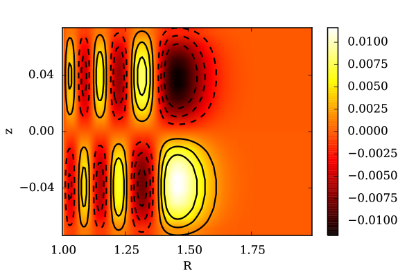
Figure 6: Color contours showing the spatial distribution in the $(r,z)$ plane of $B_{r}/B_{0}$ for the mode with $k_{z}=40$ and $n=5$ at time $t=2$. The contour lines overplot $B_{r}/B_{0}$ at time $t=0$ and show that the mode has grown unperturbed over that period. Contours are drawn from $-6\times 10^{-5}$ to $+6\times 10^{-5}$ every $2\times 10^{-5}$. Negative contours are dashed and the zero contour is omitted.

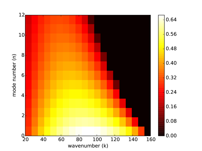
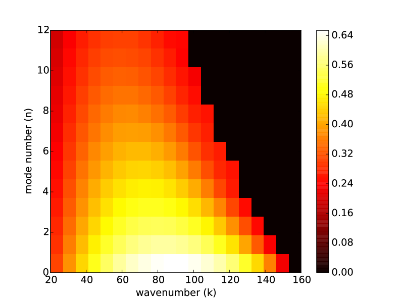
Figure 7: Growth rates of the unstable modes in the $(k_{z},n)$ plane for the case $\beta=200$ and $c_{0}=0.1$ determined using the linear analysis described in Section 2 (left panel) and using an ensemble of $240$ numerical simulations (left panel) that have a common spatial resolution $(N_{r},N_{z})=(256,16)$.

The boundary conditions we used are periodic in the vertical direction. This is possible in our setup because we neglect the density’s vertical stratification (see Section 2.1). The radial boundary conditions are more subtle to implement. As discussed earlier, the eigenmodes are confined to the inner disk. Thus, at the outer radial boundary, we force the variables to take their equilibrium, unperturbed values. At the inner boundary, we decompose the variables in the ghost cells into the sum of their equilibrium values (known analytically) and a perturbation. The latter are chosen using the first active cells of the grid with the constraint that they should satify the symmetry of the eigenmodes: zero-gradient for the vertical velocity and magnetic field perturbations and anti-symmetric for the radial and azimuthal components of the velocity and magnetic field (of course, the density perturbation vanishes). With these boundary conditions, the disk equilibrium is conserved to within machine accuracy and, as we shall see below, we can follow the MRI eigenmodes to saturation.

4.2 Linear growth

In this section, we numerically compute the growth rate of the normal modes for a vertical magnetic field whose strength is such that $\beta$, the ratio between thermal and magnetic pressure, is equal to $200$ (or, equivalently, $M_{A}=100$ given our value of the sound speed). For a given eigenmode (defined by the values of $k_{z}$ and $n$), we compute the mode’s spatial structure and theoretical growth rate as described in Section 2.4.1. At $t=0$, we add the perturbation associated with that mode to the equilibrium disk structure and start the simulation. Its amplitude is such that the maximum perturbed radial magnetic field amounts to $10^{-4}B_{0}$. The computational domain extents radially out to $r_{1}=3$ and the vertical size of the domain is set equal to the vertical wavelength of the mode. The value of $r_{1}$ is here chosen large enough to ensure that all variables reach their equilibrium value (i.e the mode amplitude goes to zero) well within the domain. In order to evaluate the amplitude of the mode during a simulation, we compute the time evolution of the volume averaged rms of the radial component of the magnetic field $B_{r}$:

$${\cal L}_{2}(B_{r})=\left(\frac{\int\!\!\!\int rB_{r}^{2}drdz}{\int\!\!\!\int rdrdz}\right)^{1/2}$$ (44)

The instantaneous growth rate $\sigma_{n}$ is then defined as the time derivative of $\log({\cal L}_{2})$. We denote by $\overline{\sigma_{n}}$ its value averaged in time over the first two orbits of the simulation (this short timescale ensures that the system remains within the linear phase).

To illustrate our general results we consider the specific mode $k_{z}=40$ and $n=5$. Its theoretical growth rate is $\sigma=0.384$. After simulating the mode’s evolution for various grid sizes, we found that a resolution of $(N_{r},N_{z})=(256,16)$ is required to capture correctly the growth rate. In this case, $\overline{\sigma_{n}}=0.380$, which corresponds to the theoretical growth rate to better than a percent. In addition, the mode structure is not modified during the linear growth. This is illustrated in Fig. 6, which shows a good correspondance between the mode spatial structure in the $(r,z)$ plane at $t=0$ (contour lines) and $t=2$ (color contours), despite an amplification by about three orders of magnitude. We note that the relative density fluctuations remain smaller than $10^{-4}$ at $t=2$, which explains the good agreement between the compressible simulation and the incompressible linear analysis. Decreasing the number of vertical cells to 8 gives $\overline{\sigma_{n}}=0.339$, and the vertical structure of the mode is incorrectly described. Likewise, when decreasing the radial resolution by a factor of two, so that $N_{r}=128$, the mode structure in the inner parts of the disk is modified, even though $\overline{\sigma_{n}}=0.371$, which is a reasonable estimate. The mode’s radial wavelength decreases inward and requires a fine resolution to be properly captured.

Based on these results, we kept a fixed resolution of $(N_{r},N_{z})=(256,16)$ and systematically evaluated $\overline{\sigma_{n}}$ for an ensemble of $240$ simulations in which we varied the vertical wavenumber $k_{z}$ between $20$ and $160$ and the mode number $n$ between $0$ and $12$. The results are summarized in Fig. 7 and show excellent agreement between the theoretical expectations (left panel) and growth rates estimated from the numerical simulations (right panel). Discrepancies occur for the slowest growing modes because they are typically overwhelmed by faster growing modes seeded by truncation errors. Except for these cases, we conclude that a finite volume compressible code can reproduce the results of the incompressible linear analysis.

4.3 Nonlinear Saturation

Figure 8: Instantaneous growth rates normalised by the theoretical growth rate as functions of $B_{r}/B_{0}$, the maximum value of the perturbed radial field. In each of the three cases $n=0$, but $k_{z}=90$ (blue curve), $k_{z}=900$ (red curve), and $k_{z}=9000$ (green curve). The corresponding plasma betas are $\beta=200,\,2\times 10^{4}$, and $2\times 10^{6}$.

We now determine what happens when the modes enter the nonlinear regime. The simulations remain axisymmetric, even though realistically the final saturated state will be non-axisymmetric. Our aim, however, is not to characterize the turbulence that follows the linear mode breakdown, a formidable task that is well beyond the scope of this paper. Rather, we ask the simpler questions: what is the amplitude of a mode when it stops growing exponentially with time? Do there exist linear modes that penetrate the nonlinear regime while maintaining their structure, as predicted in Section 3?

We performed three simulations for which $\beta=200$, $2\times 10^{4}$ and $2\times 10^{6}$. We focused on $n=0$ and select in each case a mode with growth rate close to the maximum rate, thus $k_{z}=90$, $900$ and $9000$, respectively. Note that only in the last case is $\delta$ unambigously small, being $\sim 0.05$ according to Eq. (42). The vertical and radial extent of the computational domain is changed in each of the three simulations to best accomodate each mode, as described in the previous section.

Figure 8 displays the instantaneous growth rates $\sigma_{n}$ normalized by the theoretical growth rates $\sigma$ as a function of $B_{r}/B_{0}$, where $B_{r}$ denotes here the maximum of the radial magnetic field fluctuation. Because $B_{r}/B_{0}$ increases monotonically it may be regarded as a proxy for time. The nonlinear regime corresponds to $B_{r}/B_{0}>1$. The figure clearly shows that the larger $k_{z}$, the greater the amplitude achieved by the mode before it breaks down. This is consistent with the prediction of Section 3, which states that quadratic nonlinearities intervene only once a mode grows to $\delta^{-1}$ the background. For the case $k_{z}=9000$, the estimated maximum amplitude of the perturbed field is 20, in fair agreement with Fig. 8, which shows that $\sigma_{n}/\sigma$ reaches $0.9$ at this point. This mode, in particular, has penetrated significantly into the nonlinear regime. This is not so convincingly the case for the lower $k_{z}$ modes, as expected.

In Fig. 9 we compare the distribution of the radial magnetic field at $t=0$ (top row) and at a later time when $B_{r}$ has grown to amplitudes larger than the background vertical field (bottom row) for $k_{z}=90$ and $k_{z}=9000$. The figure shows that the low $k_{z}$ mode has become strongly disturbed by $t=3.2$, whereas the field of its large $k_{z}$ counterpart retains a structure close to linear, despite possessing an amplitude 10 times greater than the background.

Finally, we check the role of compressibility, which should be important when $H<\lambda_{r}$. In code units, $H=0.1$ at $r=r_{0}$, whereas $\lambda_{r}\sim 0.1$ and $\lambda_{r}\sim 0.001$ for the two modes $k_{z}=90$ and $k_{z}=9000$. Compressibility is certainly subdominant in the breakdown of the large $k_{z}$ mode, which we attribute to quadratic nonlinearities. In the breakdown of the low $k_{z}$, on the other hand, compressibility and nonlinearity are of equal importance.

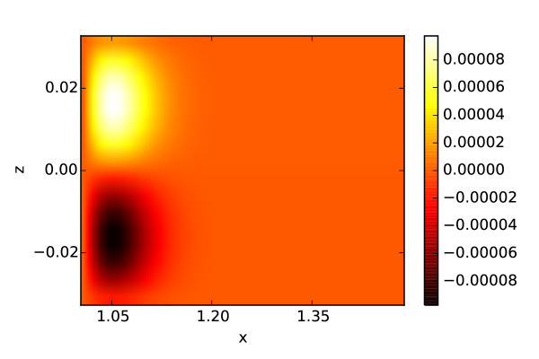
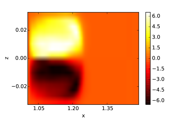
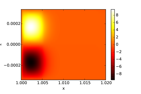
Figure 9: Color contours of $B_{r}/B_{0}$ for $k_{z}=90$, $\beta=200$ (left column) and $k_{z}=9000$, $\beta=2\times 10^{6}$ (right column) at $t=0$ (top row) and at $t=3.2$ (bottom left panel) and $2.5$ orbits (bottom right panel). By $t=2.5$, the $k_{z}=9000$ mode has grown by five orders of magnitude and is ten times larger than the background field, and yet it has retained its linear structure to a good approximation despite being well inside the nonlinear regime.

5 Conclusion

We have presented a linear analysis of the MRI in cylindrical geometry in order to make clear the connection between the global and the local theories. In particular, we show that each local channel mode corresponds to the evanescent part of a global mode. Local radially varying modes, on the other hand, correspond to sections of the same global mode at smaller radii. Moreover, we show that only global axisymmetric modes of extremely large vertical wavenumber $k_{z}$ are approximate nonlinear solutions to the governing equations. As these modes are localised to the inner boundary, most of the disk never experiences the ‘nonlinear property’ of the MRI. Direct simulations with RAMSES verify the last point, which also provides a useful numerical check on global codes generally. Our results raise a number of questions and issues, which we now list.

First, one of the most notable features of channel flows in local boxes is that they are nonlinear solutions to the governing equations. But as this property fails to appear in global disk models it is clear that this feature is an artefact of the local approximation. A natural question is then: how seriously does this artefact distort the nonlinear dynamics of the MRI in shearing boxes? It is well known that channel flows strongly influence the MRI saturation in certain circumstances (e.g. Sano & Inutsuka. 2001, Bodo et al. 2008, Lesaffre et al. 2009, Murphy & Pessah 2015). How representative of global MRI turbulence is local MRI turbulence, given the artifical prominence of channel flows in the latter?

Second, how non-local is the onset of the MRI and its ensuing turbulence in global disks? At a given radius $r_{*}$, the fastest growing disturbance is the normal mode that has its turning point there. But such a mode extends from the inner boundary $r=1$ to $r=r_{*}$, so its growth, and subsequent behaviour, may be influenced by all the shorter time-scale activity on the intervening shorter radii. Indeed, because different global modes encompass overlapping regions, significant mode-mode interactions should arise: modes that extend over large radii should interact with faster growing modes localised to small radii. Fluctuations at outer radii may be ‘slaved’ to what is going on at smaller radii. Of course, distant regions must decouple on some scale, but what sets that scale? Also how might all this be connected to global field generation and dynamo action? Such questions can only be answered by careful numerical simulations. But an understanding of the normal mode structure may provide useful clues.

Generalising the equilibrium magnetic field is another avenue to explore. Neglected in this paper, azimuthal fields are probably the dominant component in a differentially rotating flow; their importance in the disk’s stability could be reassessed in an analogous way to here. In addition, a radially varying magnetic equilibrium should also be revisited. Crucially, a vertical field that decays with radius will alter the locations of the modes’ turning points; modes of given $k_{z}$ and $n$ will extend further outward, changing the nature of the disk’s linear response.

A fourth issue regards the role of large-scale non-axisymmetric MRI modes, something we have not touched on. Such modes must contend with magnetic resonances and consequently, their localisation is more complicated than for the axisymmetric MRI (e.g. Curry & Pudritz 1996, Fu & Dong 2009). How does this influence, at all, their participation in disk turbulence?

Other topics of interest include the breakdown of the linear modes due to non-axisymmetric parasitic instabilities (Goodman & Xu 1994), which may provide an alternative pathway to saturation in some circumstances. Three-dimensional cylindrical simulations could probe their behaviour and assess their relative importance. A number of weakly non-linear analyses of the MRI have been conducted, all using local approximations (Umurhan et al. 2007, Jamroz et al. 2008, Vasil 2015). It would be interesting to test if analogous calculations are possible in a cylindrical model, using the formalism presented in this paper as the (linear) starting point. Finally, our cylindrical results could be extended to vertically structured global disk models, obviously making contact with the general theory of Terquem & Papaloizou (1996) and Ogilvie (1998), but also exploring instabilities in the strong magnetic field limit (cf. Curry & Pudritz 1995, Pessah & Psaltis 2005). The latter may be of particular interest to the magnetically arrested accretion flows around black holes recently simulated (e.g. Tchekhovskoy et al. 2011, McKinney et al. 2012).

Appendix A Mathematical derivations

A.1 Eigenvalue ordering

In this short section we sketch out a proof showing that the eigenvalues $\varepsilon$ associated with (15) are always less than 1. For simplicity the boundary conditions are taken to be either $u_{r}^{\prime}=0$ or $\partial_{r}u_{r}^{\prime}=0$ at $r=r_{1},\,r_{2}$. The proof for free boundaries is a little more involved and we omit its details.

First multiply (15) by $U^{*}$ and integrate over the domain. After integrating by parts and applying the boundary conditions the equation can be reworked into

$$\varepsilon^{-2}=\frac{\int|U|^{2}dr}{\int r^{-2q}|U|^{2}dr}+\frac{\int|\partial_{r}U|^{2}+\tfrac{3}{4}r^{2}|U|^{2}\,dr}{k_{z}^{2}\int r^{-2q}|U|^{2}dr}.$$ (45)

We see straightaway that $\varepsilon$ must be positive. But note also that $|U|^{2}>r^{-2q}|U|^{2}$ over the entire integration range and so the first term in Eq. (45) must be greater than 1. As a consequence, $\varepsilon<1$.

A.2 Eigenvalues in the large $k_{z}$ limit when $q=1$

Here we obtain approximate solutions to the eigenvalue equation $K_{\nu}(k_{z})=0$ in Section 2.4.2. In the limit of large $k_{z}$ both the order and argument of the Bessel function go to infinity. We call on the asymptotic expression given in Ferreira & Sesma (2008) for the roots of $K_{\nu}(x)$ when the order $\nu$ is large and imaginary:

$$x_{n}\approx\text{e}^{-\text{i}\pi/2}(\nu-2^{-1/3}a_{n}\text{e}^{-2\pi\text{i}/3}\nu^{1/3}).$$ (46)

Here $a_{n}$ is the $n$’th root of the Airy function $\text{Ai}(x)$. Substitution of $\nu=\text{i}k_{z}/\varepsilon$ obtains the cubic equation

$$\varepsilon-a_{n}\,2^{-1/3}k_{z}^{-2/3}\,\varepsilon^{2/3}-1=0,$$ (47)

the correct root of which can be approximated explicitly by expanding $\varepsilon$ in powers of small $k_{z}^{-2/3}$ around $1$.

References

- (1) Abramowitz, M., Stegun, I., 1964. Handbook of Mathematical Functions, Dover.
- (2) Bai, X., 2014. ApJ, 791, 137.
- (3) Balbus, S. A., Hawley, J. F., 1991. ApJ, 376, 214. (BH91)
- (4) Bodo, G., Mignone, A., Cattaneo, F., Rossi, P., Ferrari, A., 2008. AA, 487, 1.
- (5) Boyd, J. P., 2000. Chebyshev and Fourier Spectral Methods (2nd ed.). Dover Publications, New York.
- (6) Chandrasekhar, S., 1961. Hydrodynamic and Hydromagnetic Stability, Clarendon, Oxford.
- (7) Curry, C., Pudritz, R. E., Sutherland, P. G., 1994. ApJ, 434, 206.
- (8) Curry, C., Pudritz, R. E., 1995. ApJ, 354, 697.
- (9) Curry, C., Pudritz, R. E., 1996. ApJ, 281, 119.
- (10) Dubrulle, B., Knobloch, E., 1993. A&A, 274, 667.
- (11) Fabijonas, B. R., Olver, F. W. J., 1999. SIAM Review, 41, 762.
- (12) Ferreira, E. M., Sesma, J., 2008. JCoAm, 211, 223.
- (13) Flock, M., Dzyurkevich, N., Klahr, H., Mignone, A., 2010. A&A, 516, 26.
- (14) Fromang, S., Hennebelle, P., Teyssier, R., 2006. A&A, 457, 371.
- (15) Fu, W., Lai, D., 2009. ApJ, 690, 1386.
- (16) Gammie, C. F., Balbus, S. A., 1994. MNRAS, 270, 138.
- (17) Golub, G. H., Van Loan, C. F., 1996. Matrix Computations (3rd ed.). John Hopkins Uni Press, Baltimore.
- (18) Goodman, J., Xu, G., 1994. ApJ, 432, 213.
- (19) Hawley, J. F., 2001. ApJ, 554, 534.
- (20) Hawley, J. F., Guan, X., Krolik, J. H., 2011. ApJ, 738, 84.
- (21) Hawley, J. F., Richers, S. A., Guan, X., Krolik, J. H., 2013. ApJ, 772, 102.
- (22) Hirose, S., Blaes, O., Krolik, J. H., Coleman, M. S. B., Sano, T., 2014. ApJ, 787, 1.
- (23) Jamroz, B., Julien, K., Knobloch, E., 2008. AN, 329, 675.
- (24) Jiang, Y.-F., Stone, J. M., Davis, J. M., 2013. ApJ, 767, 148.
- (25) Kersalé, E., Hughes, D. W., Ogilvie, G. I., Tobias, S. M., Weiss, N. O., 2004. ApJ, 602, 892.
- (26) Kersalé, E., Hughes, D. W., Ogilvie, G. I., Tobias, S. M., 2006. ApJ, 638, 382.
- (27) Knobloch, E., 1992. MNRAS, 255, 25.
- (28) Kumar, S., Coleman, C. S., Kley, W., 1994. MNRAS, 266, 379.
- (29) Latter, H. N., Lesaffre, P., Balbus, S. A., 2009. MNRAS, 394, 715.
- (30) Latter, H. N., Fromang, S., Gressel, O., 2010. MNRAS, 406, 848.
- (31) Lesaffre, P., Balbus, S. A., Latter, H., 2009. MNRAS, 396, 779.
- (32) Lesur, G., Kunz, M. W., Fromang, S., 2014. A&A, 566, 56.
- (33) McKinney, J. C., Tchekhovskoy, A., Blandford, R. D., 2012. MNRAS, 423, 3083.
- (34) Murphy, G. C., Pessah, M. E., 2015. ApJ, 802, 139.
- (35) Ogilvie, G. I., 1998. MNRAS, 297, 291.
- (36) Okuzumi, S., Hirose, S., 2011. ApJ, 742, 65.
- (37) Papaloizou, J., Szuszkiewicz, E., 1992. GAFD, 66, 223.
- (38) Parkin, E. R., Bicknell, G. V., 2013. MNRAS, 435, 2281.
- (39) Penna, R. F., McKinney, J. C., Narayan, R., Tchekhovsky, A., Shafee, R., McClintock, J. E., 2010. MNRAS, 408, 752.
- (40) Pessah, M. E., Psaltis, D., 2005. ApJ, 628, 879.
- (41) Pessah, M. E., Goodman, J., 2009. ApJ, 698, 72.
- (42) Riley, K. F., Hobson, M. P., Bence, S. J., 2006. Mathematical Methods for Physics and Engineering, 3rd edition. Cambridge Uni. Press.
- (43) Rosin, M., Mestel, A. J., 2012. MNRAS, 425, 74.
- (44) Sano, T., Inutsuka, S., 2001. ApJ, 561, 179.
- (45) Tchekhovskoy, A., Narayan, R., McKinney, J. C., 2011. MNRAS, 418, L79.
- (46) Terquem, C., Papaloizou, J. C. B., 1996. MNRAS, 279, 767.
- (47) Teyssier, R., 2002. A&A, 385, 337.
- (48) Umurhan, O. M, Regev, O., Menou, K., 2007. PRL, 98, 4501.
- (49) Vasil, G. M., 2015. Proc. R. Soc. A, 471, 20140699.
- (50) Velikhov, E., 1959. Sov. Phys. -JETP, 36, 1398.