Multidimensional Discrete Compactons in Nonlinear Schrödinger Lattices with Strong Nonlinearity Management

Abstract

The existence of multidimensional lattice compactons in the discrete nonlinear Schrödinger equation in the presence of fast periodic time modulations of the nonlinearity is demonstrated. By averaging over the period of the fast modulations, a new effective averaged dynamical equation arises with coupling constants involving Bessel functions of the first and zeroth kind. These terms allow one to solve, at this averaged level, for exact discrete compacton solution configurations in the corresponding stationary equation. We focus on seven types of compacton solutions: single site and vortex solutions are found to be always stable in the parametric regimes we examined. Other solutions such as double site in- and out-of-phase, four site symmetric and anti-symmetric, and a five site compacton solution are found to have regions of stability and instability in two-dimensional parametric planes, involving variations of the strength of the coupling and of the nonlinearity. We also explore the time evolution of the solutions and compare the dynamics according to the averaged with those of the original dynamical equations without the averaging. Possible observation of compactons in the BEC loaded in a deep two-dimensional optical lattice with interactions modulated periodically in time is discussed.

I Introduction

Periodic management of parameters of nonlinear lattices (and continua) is a very attractive technique for the generation of new types of systems or excitations with interesting localization properties Malomed_book . For example, dynamic suppression of (atom and light, respectively) interwell tunneling has been reported experimentally in Bose-Einstein condensates arimondo and in optical waveguide arrays szameit . On the other hand, very fast periodic time variation of the nonlinearity, also called the strong nonlinearity management (SNLM) technique, has been recently shown to be quite effective towards inducing compactly supported (so-called compacton) solutions in lower dimensional discrete systems such as one dimensional (1D) one and two component Bose-Einstein condensates (BECs) in optical lattices or arrays of nonlinear optical waveguides described by the discrete nonlinear Schrödinger (DNLS) equation AKS010 ; AHSU14 . The main feature of such solutions, unlike other types of nonlinear excitations such as discrete breathers and intrinsic localized modes, is that their amplitudes decay to zero sharply without any tails. It has been shown for the 1D case that the lack of exponential tails is a consequence of the nonlinear dispersive interaction induced by the SNLM which permits the vanishing of the intersite tunneling at compacton edges. The absence of tails imply that compactons cannot interact with each other until they are in contact. In the lattice realm, this potentially allows for the possibility of “maximal localization” in the form of a single site solution.

Compactons are quite generic in nonlinear continua rosenau ; rosenau2 (in one and also higher Ros1 dimensions) and lattices konotop1999 ; kevrekidis2002 (including compact breathers flach ) bearing nonlinear dispersion. The difficulty of implementing this condition in physical contexts has largely restricted the investigations mainly to the mathematical side, although this situation is now rapidly evolving. Besides Bose-Einstein condensates under SNLM, physical compactons were suggested to appear also in exciton-polariton condensates konotop2013 and nearly-compact (doubly exponential) traveling waves have also been identified in the realm of granular crystals bearing purely nonlinear interactions atanas . Finally, another area of significant interest has recently arisen where special solutions in the form of discrete compactons may emerge. This is due to the existence of so-called flat bands in the linear dispersion relation (due to the geometric characteristics of the corresponding lattice, such as e.g. the Kagomé lattice) rodrig1 . A realization of this type emerged very recently in the realm of the so-called Lieb photonic lattices Molina2015 .

Among the above different (Klein-Gordon, nonlinear Schrödinger, Fermi-Pasta-Ulam, etc.) model equations in which compactly supported structures have been proposed DNLS ones are, arguably, of the most widely applicable as models both for BECs and for nonlinear optics. In the presence of SNLM, this type of system supports discrete compactons via a site-dependent nonlinear rescaling of the inter-well tunneling (see AKS010 for details). A similar approach, applied to the quantum version of the DNLS model, i.e., to the Bose-Hubbard model with time dependent onsite interaction, has been shown to be quite effective for creating new quantum phases in BECs with compacton-type excitations Rapp ; Gres1 as well as for the generation of density dependent synthetic gauge fields Gres2 .

These studies have mainly focused on the one dimensional case. On the other hand, it is known that compactons can exist also in multidimensional contexts. In particular, multidimensional compactons have been investigated in continuous models such as (two-dimensional) variants of the Korteweg–de Vries equations with nonlinear dispersion Ros1 , relativistic scalar field theories in two dimensions Bazeia , Klein-Gordon and nonlinear Schrödinger equations with sub-linear forces, etc.. In these last cases, however, the mechanism leading to compacton formation is not the nonlinear dispersion but the presence of a sub-quadratic interaction potential which enforces compact patterns with sharp fronts Ros2 ; Ros3 . In this context, existence of vortex compactons was also demonstrated to be possible, although only with a finite lifetime Ros3 .

In the discrete case, multidimensional compactons have been scarcely investigated and only in the special case example of compact coherent structures in the presence of a flat band of the linear spectrum rodrig1 ; Molina2015 . To the best of our knowledge, general case examples (different numbers of sites, including ones bearing vorticity) of multidimensional discrete compactons of the nonlinear Schrödinger type, amenable to physical applications in BECs and nonlinear optics, have not yet been investigated.

The aim of this paper is to demonstrate and systematically explore the existence and stability of multidimensional lattice compactons in the discrete nonlinear Schrödinger equation in the presence of periodic time modulations of the nonlinearity i.e., in a 2-dimensional generalization of AKS010 bearing the potential for a wide range of additional structures. In this work we concentrate mainly on compactons localized on no more than five interacting neighboring sites of a two-dimensional (2D) square lattice; of particular interest, in addition to the stable single site compacton, is the stable four site compacton vortex solution i.e., bearing a vortical phase structure. In particular, the existence and stability properties of DNLS compacton excitations are investigated both for generic time dependent nonlinear modulations and in the SNLM limit for which an effective averaged DNLS model is derived. We show that single site compactons are stable in the whole parameter space, however, two site compactons have finite stability ranges (although bearing some nontrivial differences from the “standard” DNLS model), different for symmetric and anti-symmetric types and with different dynamical features. Interestingly, stationary three site compactons with real amplitude cannot exist in the square geometry, while four site compactons of the symmetric or anti-symmetric types exist but have finite regions of instability similar to the double site configurations. On four nearest-neighboring sites, however, for all values in the parameter space one has a stable vortex compacton in which the phase of the wavefunction increases by $\pi/2$ moving clockwise from one corner to the next of the square. Since compactons interact only when they are in contact, one can obviously construct arbitrary single and two site compacton patterns by placing them on non interacting sites (such as for example next-neighboring sites along a diagonal). We also show that five site compactons with $C_{4}$ symmetry can exist and can be stable; their regions of instability are finite, similar to other configurations’ instability.

The paper is organized as follows. In section II we introduce the model equation of a 2D DNLS with SNLM and discuss the theoretical derivation of the effective averaged equations with nonlinear dispersion. In section III we derive the existence conditions for exact compacton solutions of the averaged DNLS equation and in section IV we study numerically the linear stability properties and compare results with direct numerical integrations of the original (unaveraged) DNLS system. In the last section we discuss briefly the potential future experimental implementations, summarize our main results and provide some pointers for future work.

II Model and Theoretical Setup

Consider the following 2D DNLS equation pgk_book

$$i\dot{u}_{n,m} + k(u_{n+1,m}+u_{n-1,m}){\ +\ }\tilde{k}(u_{n,m+1}+u_{n,m-1})$$ (1)

$$+(\gamma_{0}+\gamma(t))|u_{n,m}|^{2}u_{n,m}=0,$$

which serves as a model for the dynamics of BEC in optical lattices subjected to SNLM (through varying the interatomic scattering length by external time dependent magnetic fields via a Feshbach resonance) ABKS , as well as for light propagation in 2D optical waveguide arrays Assanto . In the latter case, where this type of modulation has been realized not only in discrete but also in continuum media (in both one and higher dimensions) pgk2 , the evolution variable is the propagation distance. Hence, here the SNLM consists of periodic space variations of the Kerr nonlinearity along the propagation direction with the coupling constants $k,\tilde{k}$ quantifying the tunneling between adjacent sites along $n$ and $m$ directions, respectively, $\gamma_{0}$ denoting the onsite constant nonlinearity and $\gamma(t)$ representing the time dependent modulation (of the interatomic interactions or of the refractive index, in atomic and optical settings, respectively). In the following we assume a strong management case with $\gamma(t)$ being a periodic, e.g. $\gamma(t)=\gamma(t+{T_{0}})$, and rapidly varying function. As a prototypical example, we use $\gamma(t)=\frac{\gamma_{1}}{\varepsilon}\cos(\Omega\tau)$, with $\gamma_{1}\sim O(1)$, $\varepsilon\ll 1$, $\tau=t/\varepsilon$ denoting the fast time variable and $T=2\pi/\Omega$ the period with respect to $\tau$ ($T_{0}=\varepsilon T$). In the following we take, for simplicity, the coupling constants $k,\tilde{k}$ to be the same for the two directions (assuming square symmetry): $k=\tilde{k}\equiv\kappa$.

The existence of compacton solutions of Eq. (1) in the SNLM limit can be inferred from (and analyzed in the context of) an effective averaged 2D DNLS equation obtained by averaging out the fast time $\tau$. To that effect, it is convenient to perform the transformation JKP $u_{n,m}(t)=v_{n,m}(t)e^{i\Gamma|v_{n,m}(t)|^{2}}$ with $\Gamma{\ =\int_{0}^{t}dt\ \gamma(t)}=\gamma_{1}\Omega^{-1}\sin(\Omega\tau)$, which allows one to rewrite Eq. (1) as

$$i\dot{v}_{n,m}=\Gamma v_{n,m}(|v_{n,m}|^{2})_{t}-\kappa X{\ -\ }\gamma_{0}|v_{n,m}|^{2}v_{n,m},$$ (2)

with

$$X = v_{n+1,m}e^{i\Gamma\theta^{m}_{+}}+v_{n-1,m}e^{i\Gamma\theta^{m}_{-}}+v_{n,m+1}e^{i\Gamma\theta^{+}_{n}}$$ (3)

$$+v_{n,m-1}e^{i\Gamma\theta^{-}_{n}},\mbox{ and }$$

$$\theta^{m}_{\pm} = |v_{n\pm 1,m}|^{2}-|v_{n,m}|^{2},\;\;\theta^{\pm}_{n}=|v_{n,m\pm 1}|^{2}-|v_{n,m}|^{2}.$$

On the other hand, ${(|v_{n,m}|^{2})_{t}=(\dot{v}_{n,m}v_{n,m}^{*}+v_{n,m}\dot{v}_{n,m}^{*})}=i\kappa(v_{n,m}^{*}X-v_{n,m}X^{*})$, with the star denoting complex conjugation. Substituting this expression into Eq. (2) and averaging the resulting equation over the period $T$ of the rapid modulation, we obtain

$$i\dot{v}_{n,m} = i\kappa|v_{n,m}|^{2}\langle\Gamma X\rangle-i\kappa v_{n,m}^{2}\langle\Gamma X^{*}\rangle-\kappa\langle X\rangle$$ (4)

$${\ -\ }\gamma_{0}|v_{n,m}|^{2}v_{n,m},$$

with $\langle\cdot\rangle\equiv\frac{1}{T}\int_{0}^{T}(\cdot)d\tau$ denoting the fast time average. The averaged terms in Eq. (4) can be calculated by means of the elementary integrals ${\langle e^{i\Gamma\theta_{\pm}}\rangle=J_{0}(\alpha\theta_{\pm})}$, $\;\langle\Gamma e^{\pm i\Gamma\theta_{\pm}}\rangle=\pm i\alpha J_{1}(\alpha\theta_{\pm})$, with $J_{i}$ being Bessel functions of order $i=0,1$ and $\alpha=\gamma_{1}/\Omega$, thus giving

$$i\dot{v}_{n,m}{=F(v)}$$ (5)

with

$${F(v)}=-\gamma_{0}|v_{n,m}|^{2}v_{n,m}$$

$$-\alpha\kappa v_{n,m}[(v_{n+1,m}v_{n,m}^{\ast}+v_{n+1,m}^{\ast}v_{n,m})J_{1}(\alpha\theta^{m}_{+})$$

$$+(v_{n,m+1}v_{n,m}^{\ast}+v_{n,m+1}^{\ast}v_{n,m})J_{1}(\alpha\theta^{+}_{n})$$

$$+(v_{n-1,m}v_{n,m}^{\ast}+v_{n-1,m}^{\ast}v_{n,m})J_{1}(\alpha\theta_{-}^{m})$$

$$+(v_{n,m-1}v_{n,m}^{\ast}+v_{n,m-1}^{\ast}v_{n,m})J_{1}(\alpha\theta^{-}_{n})]$$ (6)

$$-\kappa[v_{n+1,m}J_{0}(\alpha\theta_{+}^{m})+v_{n,m+1}J_{0}(\alpha\theta^{+}_{n})$$

$$+v_{n-1,m}J_{0}(\alpha\theta_{-}^{m})+v_{n,m-1}J_{0}(\alpha\theta^{-}_{n})].$$

Note that the parameters $\gamma_{1},\Omega{\ \sim O(1)}$, and the averaged equation is valid for times $t\leq 1/\epsilon$. This modified DNLS equation can be written as $i\dot{v}_{n,m}=\delta H_{av}/\delta v_{n,m}^{\ast},$ with the averaged Hamiltonian

$$H_{av}=-\sum_{n,m}\{\kappa J_{0}(\alpha\theta_{+}^{m})\left[v_{n+1,m}v_{n,m}^{\ast}+v_{n+1,m}^{\ast}v_{n,m}\right]$$

$$+\kappa J_{0}(\alpha\theta^{+}_{n})\left[v_{n,m+1}v_{n,m}^{\ast}+v_{n,m+1}^{\ast}v_{n,m}\right]+\frac{\gamma_{0}}{2}|v_{n,m}|^{4}\}.$$

It is interesting to note that this Hamiltonian, except for the rescaling of the coupling constants $k\rightarrow\kappa J_{0}(\alpha\theta_{+}^{m})$, $\tilde{k}\rightarrow\kappa J_{0}(\alpha\theta^{+}_{n})$, is the same as the Hamiltonian of the DNLS equation in absence of SNLM (e.g. with $\gamma_{1}=0$). A similar rescaling was reported also for the 1D case AKS010 .

It is also worth noting that while the appearance of the Bessel function is intimately connected with harmonic modulations, the existence of compacton solutions and the lattice tunneling suppression is generic for periodic SNLM.

The generalization of these equations to the case of 3D DNLS with cubic lattice symmetry is also quite straightforward to derive (omitted here for brevity). In our numerical results below, we will restrict our considerations to the numerically more tractable 2D case (also more physically realistic at least in the optics realm where the $z$-direction plays the role of the propagation direction).

III Exact 2D compactons

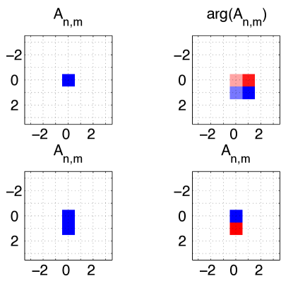
Figure 1: (color online) We plot typical examples of exact 2D compacton solutions of Eq. (7). In the top left panel we show a single site solution, in the bottom left we show a double-site in-phase solution, and in the bottom right, we show a double-site out-of-phase solution. In these three plots colors show the (real) values of $A_{n,m}$ where blue represents $A_{n,m}=A_{0}$ and red $A_{n,m}=-A_{0}$. No color represents zero amplitude. In the top right plot we show a vortex solution where the four central colored sites all have amplitude $A_{0}$, and $arg(v_{n,m})\in\{-\pi/2,0,\pi/2,\pi\}$ is plotted by the four respective colors: dark red (at $(n,m)=(0,1)$), light red (at $(n,m)=(0,0)$), light blue (at $(n,m)=(1,0)$), dark blue (at $(n,m)=(1,1)$). Here the length and width of the 2D grid are each $L=7$.

To demonstrate the existence of exact compactons in the averaged system, we seek stationary solutions of the form $v_{n,m}=A_{n,m}e^{-i\mu t}$ with $A_{n,m}\in\mathbb{C}$ for which Eq. (5) becomes

$${\mu A_{n,m}=F(A)}$$ (7)

for $F$ given by Eq. (6). In the following, we theoretically predict and numerically verify that exact solutions of this equation can exist in the form of genuine compactons i.e., possessing vanishing tails.

To search for compacton solutions, we begin by applying (7) at any zero-amplitude site that has exactly one out of its four neighbors nonzero. We label this nonzero site $A_{N,M}\neq 0$ and we call it an “edge site” of the compacton. For $\kappa\neq 0$, this gives the condition

$$J_{0}(\alpha|A_{N,M}|^{2})=0\quad\Rightarrow\quad|A_{N,M}|^{2}=z_{j}/\alpha$$ (8)

where $z_{j}$ is the $j^{th}$ zero of the Bessel function $J_{0}$. In other words, each edge site of the compacton has amplitude

$$A_{0}\stackrel{{\scriptstyle def.}}{{=}}\sqrt{z_{j}/\alpha}.$$ (9)

Applying (7) at edge site(s) of the compacton gives additional condition(s) that depend on the shape of the compacton. We will focus on the following shapes although other configurations are possible: a single site, a double site in-phase, a double site out-of-phase, three types of four site solutions in the form of symmetric, asymmetric and vortex excitations, and finally a five site configuration. Figures 1 and 2 show one example of each of these configurations. $L$ represents the horizontal (and vertical) length of the lattice.

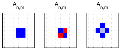
Figure 2: (color online) The plots show three additional examples of exact 2D compacton solutions of Eq. (7) on four and five lattice sites. In the left and middle panels symmetric and anti-symmetric four site compactons are shown, respectively, while the right panel depicts a five site compacton. Dark blue and red colors represent $A_{n,m}=A_{0}$ and $A_{n,m}=-A_{0}$ similar to the single and double site plots in Figure 1. The light blue color at the center of the right-most plot represents the value $y$ for the center site of the five site solution obtained from Eq. (16). Axis labels are the same here as those seen in Figure 1.

For a single site compacton solution located at $(n_{0},m_{0})$, this nonzero site is an edge site so it has amplitude $A_{0}$. Taking $A_{n_{0},m_{0}}=A_{0}$ and applying (7) at $(n_{0},m_{0})$ gives the value

$$\mu=-\gamma_{0}A_{0}^{2}.$$ (10)

It is interesting to notice that this solution coincides with the one obtained for the one dimensional DNLS under SNLM in AKS010 . This is due to the fact that for a single site the compact nature of the solution does not allow it to distinguish 1D from 2D or even 3D (this is true for a 3D cubic lattice as well). Similar to the 1D case the single site compactons are stable; we will see this in more detail in Section 4.

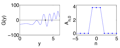
Figure 3: (color online) Graphical solution of Eq. (16) written as $G(y)=0$ (left panel) and section at $m=0$ of a five-site compacton (right panel) of Eq. (7) for parameter values $\kappa=0.5,\alpha=1,\gamma_{0}=2$ with amplitudes at edges sites fixed in correspondence of the fifth zero, $z_{5}$, of the Bessel function $J_{0}$, e.g. $A_{0}=\sqrt{z_{5}/\alpha}\approx 3.864$. The amplitude of the central site is taken as the zero of G(y) at $y\approx 3.8695$ (black dot in the left panel) while the corresponding chemical potential is obtained from Eq. (15) as $\mu\approx-30.678$.

For a double-site compacton located at $(n_{0},m_{0})$ and $(n_{0}+1,m_{0})$ (or any other adjacent pair of indices) each with amplitude $A_{0}$ there are the two possibilties: $A_{n_{0}+1,m_{0}}=\pm A_{n_{0},m_{0}}$ where plus denotes an in-phase solution and minus an out-of-phase solution. Using that $J_{1}(0)=0$ and $J_{0}(0)=1$, application of (7) at either of the two nonzero sites then gives the value

$$\mu=\mp\kappa-\gamma_{0}A_{0}^{2}$$ (11)

where the minus corresponds to the in-phase solution and the plus to the out-of-phase solution.

From the above cases one could expect that, although with different stability properties, 1D compactons located on the lattice along $n$ or $m$ directions could be also solutions of multidimensional lattices. This however, except for the cases considered above, is not true in general. In this respect, one and two-sites compactons are very special, since the number of edge sites in these solutions does not change with dimensionality their analytical expressions remain the same in 1D, 2D and 3D. For compactons with more than two sites, however, this is not true. Thus, for three-site compacton with real amplitudes $(...,0,A_{1},A_{2},A_{1},0,...)$, in the $n$ direction and zero amplitudes in all other sites, for example, one has three edge sites in 2D but only two in 1D. In contrast with the 1D case, where solutions with real amplitudes exist for arbitrary choices of parameters and are stable AKS010 , the constraints resulting from Eq. (7) can be satisfied only for particular choices of parameters, e.g. real amplitude three-site compactons of 2D DNLS under SNLM are not generic solutions in parameter space. The situation is different for complex and an example of this type will, in fact, be given below.

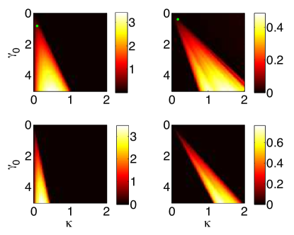
Figure 4: (color online) We plot $\max({\rm real}(\nu))$ in order to show the strength of the instabilities and regions of stability. Parameter values common across all four plots are $\epsilon=0.01$ and $\Omega=\gamma_{1}=10$ so that $\alpha=1$. The left column of plots is associated with a double site in-phase solution with lattice length both horizontally and vertically $L=17$. The right column of plots is associated with a double site out-of-phase solution with lattice length $L=15$. The top row corresponds to $j=1$ and the bottom to $j=2$. Notice that the top right plot shows more striations in the coloring than the top left plot; these further smooth out with higher lattice size $L$. The green dots in the top two plots are parameter values for which the unstable solutions are propagated in time; see Figures 7, 8 below.

Genuine 2D compacton solutions first occur on four neighboring sites of a lattice cell. These square compactons can be either symmetric or anti-symmetric (see the panels of Fig. 2). In either case all four nonzero sites are edge sites with amplitude $A_{0}$. Denoting with $(n_{0},m_{0})$ the coordinates of the upper left corner of the four site compacton, the symmetric solution has plus signs on the four nonzero sites so that

$$A_{n_{0},m_{0}}=A_{n_{0}+1,m_{0}}=A_{n_{0},m_{0}+1}=A_{n_{0}+1,m_{0}+1}=A_{0}.$$

The anti-symmetric solution has an alternating pattern of plusses and minuses of the form

$$A_{n_{0},m_{0}}=A_{n_{0}+1,m_{0}+1} = A_{0},$$

$$A_{n_{0}+1,m_{0}}=A_{n_{0},m_{0}+1} = -A_{0},$$

with vanishing amplitudes, $A_{n,m}=0$, on all other sites. Substituting the above expressions into Eq. (7) one readily gets the following equation for $\mu$ to be satisfied

$$\pm 2k+A_{0}^{2}\gamma_{0}+\mu=0$$ (12)

with the signs plus and minus referring to the symmetric and anti-symmetric case, respectively.

Quite remarkably, the DNLS system under SNLM can also support discrete vortex-compactons, an unprecedented feature of earlier two-dimensional (continuous or discrete) compacton considerations. In particular, for a $2\times 2$ shaped vortex solution with the top left nonzero site located at index $(n_{0},m_{0})$, all four sites are edge sites with amplitude $A_{0}$. Then we can write

$$A_{n_{0},m_{0}}=A_{0},\qquad A_{n_{0},m_{0}+1}=A_{0}e^{-i\pi/2}$$ (13)

$$A_{n_{0}+1,m_{0}}=A_{0}e^{i\pi/2},\qquad A_{n_{0}+1,m_{0}+1}=A_{0}e^{i\pi}$$

and (7) applied on any of the four vortex sites gives

$$\mu=-\gamma_{0}A_{0}^{2}.$$ (14)

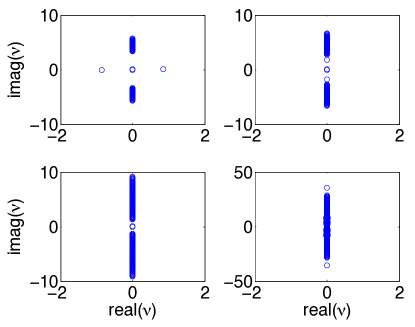
Figure 5: (color online) The panels show eigenvalues in the complex plane for selected parameters corresponding to a horizontal cut on the top left panel of Figure 4 (in-phase solution), obtained by setting $\gamma_{0}=1.75$. For $\kappa=0$ (not shown) the eigenvalues are purely imaginary and four eigenvalues are zero. For small nonzero $\kappa$ there are only two zero eigenvalues and the other two previously zero eigenvalues have begun to increase in magnitude on the real axis; this is shown for $\kappa=0.3$ in the top left panel. As $\kappa$ increases the solution stabilizes and these real eigenvalues move back towards zero horizontally along the real axis. For even higher $\kappa$ values (at which the solution remains stable), the two eigenvalues increase in magnitude again from zero, but this time along the imaginary axis; this is shown for $\kappa=0.5$ in the upper right panel. These eigenvalues merge with the band of eigenvalues on the imaginary axis meanwhile the (continuous spectrum) band lengthens; this is shown for $\kappa=1$ in the bottom left panel. At even higher $\kappa$ values, two complex conjugate purely imaginary eigenvalues emerge from the band at a magnitude higher than any eigenvalue in the band; this is depicted in the lower right panel for $\kappa=5$. The eigenvalues in the bottom right panel that appear to have very small nonzero real part are seen to actually have zero real part when the eigenvalues are computed for a much higher lattice length $L$.

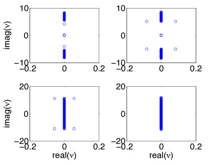
Figure 6: (color online) The panels show the eigenvalues in the complex plane for selected parameters corresponding to a horizontal cut on the top right panel of Figure 4 (out-of-phase solution), obtained by setting $\gamma_{0}=3$. For $\kappa=0$ (not shown) the eigenvalues are purely imaginary and four eigenvalues are zero. For small nonzero $\kappa$ there are only two zero eigenvalues and the other two previously zero eigenvalues have begun to increase in magnitude on the imaginary axis; this is shown for $\kappa=0.35$ in the top left panel. After the two merge with the (continuous spectrum) band of eigenvalues on the imaginary axis a quartet of complex eigenvalues then emerges for higher $\kappa$; this is depicted for $\kappa=0.45$ in the top right panel. For higher $\kappa$ values the four complex eigenvalues move in the complex plane, first increasing in real and imaginary parts then decreasing in real part until they merge again with the imaginary axis (meanwhile the continuous spectrum band on the imaginary axis lengthens); the bottom two plots show this restabilization with $\kappa=1.38$ in the bottom left and $\kappa=1.45$ in the bottom right. At even higher $\kappa$ values (at which the solution remains stable) two complex conjugate purely imaginary eigenvalues emerge from the band at a magnitude higher than any eigenvalue in the band, similar to the lower right panel of Figure 5.

With some additional effort it is possible to obtain exact compacton solutions involving more ($>4$) nonzero sites. As an example, consider the case of a five site compacton shaped as in the right panel of Fig. 2. Let $(n_{0},m_{0})$ denote the index of the center site of the configuration and define $y\equiv A_{n_{0},m_{0}}$. The four edge sites of the five site solution have amplitudes $A_{0}$ so we take $A_{n_{0}+1,m_{0}}=A_{n_{0}-1,m_{0}}=A_{n_{0},m_{0}+1}=A_{n_{0},m_{0}-1}=A_{0}$. Notice that the four edge sites (dark blue in the right panel of Fig. 2) isolate the central (light blue) site from the bulk, reproducing the same situation occurring for a three-site compacton in 1D (in 3D a similar solution would imply a seven-site compacton). Plugging the above edge site expressions into Eq. (7), applied at any one of the four edge sites, then gives an expression fixing the chemical potential

$$\mu(y)=-\kappa\frac{y}{A_{0}}J_{0}(\xi(y))-\gamma_{0}A_{0}^{2}+2\,\alpha\,\kappa\,A_{0}\,y\,J_{1}(\xi(y)),$$ (15)

where $\xi(y)=\alpha(A_{0}^{2}-y^{2})$. The final constraint is obtained by applying Eq. (7) at the center site $(n_{0},m_{0})$. Combining the result with the expression in Eq. (15) for $\mu$ shows that the amplitude $y$ at the center site must be a solution of the equation $G(y)=0$ for

$$G(y) \equiv \kappa\left(\frac{4A_{0}}{y}-\frac{y}{A_{0}}\right)J_{0}(\xi(y))-\frac{\gamma_{0}}{\alpha}\xi(y)$$ (16)

$$+10\,\alpha\kappa\,A_{0}\,y\,J_{1}(\xi(y)).$$

Although Eq. (16) does not yield a simple analytical expression for $y$, it can be easily solved numerically providing an exact five-site compacton with chemical potential given by Eq. (15). In general, for fixed parameters and a fixed value for $A_{0}=\sqrt{z_{n}/\alpha}$, more than one zero can exist for G (see left panel of Fig. 3), although not all of them necessarily lead to stable compactons. It is remarkable, however, that some of them can have non-vanishing intervals/ranges of stability in parameter space. We now turn to the details of the stability considerations.

IV Stability analysis and numerical simulations

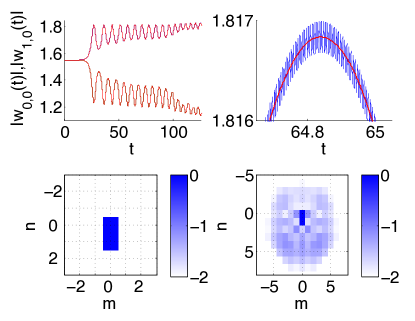
Figure 7: (color online) The plots show the result of propagation of the double site in-phase exact compacton solution in the time parameter $t$ according to each of the equations (1) and (5). The values of $\epsilon,\Omega,\gamma_{1},\alpha$ are the same as in Figure 4; these values give $A_{0}\approx 1.5507$ for $j=1$ through Eq. (9). In the bottom left panel the plot shows $\log_{10}(|u_{n,m}(0)|)$ plotted as a function of $n,m$ where $u_{n,m}(0)=v_{n,m}(0)$ is the initial double site in-phase compacton configuration at $t=0$; this plot, of course, shows an order 0 logarithmic amplitude at the two excited sites and vanishing amplitude elsewhere. The instability strength for this solution is $\max({\rm real}(\nu))\approx 0.5327$. In the bottom right panel the plot shows $\log_{10}(|v_{n,m}(120)|)$ where $v_{n,m}(t)$ is determined from $v_{n,m}(0)$ according to the averaged equation (5); the plot of $\log_{10}(|u_{n,m}(120)|)$ determined from the non-autonomous equation (1) is visually indistinguishable from the averaged version shown in the bottom right. In the bottom right plot we see small amplitude excitations appearing near the compacton site, and these small amplitudes continue to spread out spatially as $t$ increases, while the central sites have amplitudes which approach nonzero values. The top left panel shows this evolution of the amplitude of the two excited sites over time with the unaveraged magnitudes $|w_{0,0}(t)|={|u_{0,0}(t)|}$ in blue and $|w_{1,0}(t)|={|u_{1,0}(t)|}$ in green; these are propagated according to (1). The overlying red line plots correspond to the magnitudes $|w_{0,0}(t)|={|v_{0,0}(t)|}$, $|w_{1,0}(t)|={|v_{1,0}(t)|}$ propagated according to the averaged equation (5). From the perspective displayed in the upper left panel the averaged and the unaveraged amplitudes seem to lie on top of one another. The top right panel here shows a small portion of the same plot zoomed in so as to show how the averaged solution in red in fact averages the non-autonomous equation solution (over a period of the nonlinearity prefactor variation) in blue.

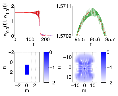
Figure 8: (color online) These plots are similar to those in Figure 7 but here for the double site out-of-phase compacton solution; also the bottom right panel here corresponds to $t=180$. The values of $\epsilon,\Omega,\gamma_{1},\alpha$ are the same as those seen in Figure 4 for the double site out-of-phase case. These values again give $A_{0}\approx 1.5507$ for $j=1$ by (9). The instability strength for this solution is $\max({\rm real}(\nu))\approx 0.0298$. Notice that here, the eventual evolution leads to a single-site excitation (see the amplitude evolution in the top left and the eventual profile in the bottom right).

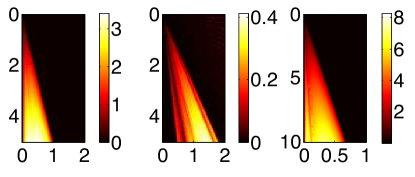
Figure 9: (color online) We plot $\max({\rm real}(\nu))$ in order to show the strength of the instabilities and regions of stability. Parameter values common across all four plots are $L=11$, $\epsilon=0.01$ and $\Omega=\gamma_{1}=10$ so that $\alpha=1$. The left-most plot is associated to a four site symmetric solution using the first zero of the Bessel function with $j=1$, the middle plot corresponds to a four site asymmetric solution with $j=1$, and the right-most plot is for the five site solution with $j=5$. The axis labels are the same as those established in Figure 4.

In order to examine stability of the solutions found in Section III we set

$$v_{n,m}(t)=\left(A_{n,m}+\delta e^{\nu t}\psi_{n,m}\right)e^{-i\mu t}$$ (17)

where both $A_{n,m}$ and $\psi_{n,m}$ are independent of time $t$. One can then show that for $\psi_{n,m}=a_{n,m}+ib_{n,m}$ the real vector $\left(\begin{array}[]{c}a_{n,m}\\ b_{n,m}\end{array}\right)$ (with $2L^{2}$ components) is an eigenvector of the $2L^{2}\times 2L^{2}$ matrix

$$M=\left[\begin{array}[]{cc}-\frac{\partial Im(F(\psi))}{\partial a}&-\frac{\partial Im(F(\psi))}{\partial b}\\ &\\ \frac{\partial Re(F(\psi))}{\partial a}&\frac{\partial Re(F(\psi))}{\partial b}\end{array}\right]$$ (18)

with eigenvalue $\nu$.

We find that the single site and vortex solutions are stable for all parameter values $\kappa,\lambda_{0}$ so that $\max({\rm real}(\nu))=0$; in other words, the nonzero sites’ time evolution plots according to the averaged Eq. (5) even under perturbation does not lead to growth. The time evolution of the single site or vortex solution according to the original Eq. (1) with the time-periodic nonlinearity gives the expected result of oscillations about the stable solution given by the averaged equation. The double site solutions have regions of instability which depend on the system’s parameters. Figure 4 shows the maximal growth rate of the instability as a function of the dc strength of the nonlinearity and of the coupling constant. We see that the in-phase solutions present instability intervals near the uncoupled limit (but contrary to what is the case in the regular DNLS, these instability intervals end at a finite value of the coupling). On the other hand, for the out-of-phase solutions, the instability intervals arise for an intermediate range of the couplings, a feature to which we will return below. Interestingly, we also find that an increase in the index $j$ of the zero of the Bessel function $J_{0}$ decreases the size of the region of instability. Additional analysis has shown that for the double site in-phase, an increase in the parameter $\alpha$ (i.e. decrease in frequency $\Omega/2\pi$ of the $\gamma$ function) decreases the size of the region of instability when plotted versus the coupling $\kappa$, and the dc nonlinearity strength $\gamma_{0}$ as in Figure 4. For the double site out-of-phase, an increase in the parameter $\alpha$ (i.e. decrease in frequency $\Omega/2\pi$ of the $\gamma$ function) expands the region of instability when plotted versus $\kappa,\gamma_{0}$ as in Figure 4.

The nature of the double site instabilities is more clearly demonstrated in Figures 5, 6. For the double site in-phase solutions, unstable eigenvalues constitute a pair of equal in magnitude and opposite real numbers; see Figure 5 where more details of the transition between stable and unstable are discussed. A key feature of the double site in-phase (in)stability is that for fixed $\gamma_{0}$, small nonzero $\kappa$ values give unstable solutions and higher $\kappa$ values stabilize the solution, a feature that is typically absent in the standard DNLS model. For the double site out-of-phase solutions, unstable eigenvalues appear as a quartet (due to the Hamiltonian nature of the system), i.e. two complex conjugate pairs with equal magnitude plus/minus real parts. This arises from the collision of the two imaginary eigenvalues (in this case), stemming from the origin with the continuous spectrum, a feature that is common in such out-of-phase focusing nonlinearity settings; see e.g. pgk_book . More details of the transitions between stable and unstable solutions for the out-of-phase solutions are discussed in Figure 6. A key feature of the double site out-of-phase (in)stability is that for fixed $\gamma_{0}$, both small nonzero and large positive $\kappa$ values give stable solutions with the unstable region lying in a finite $\kappa$ interval that lies away from $\kappa=0$. For large $\kappa$, the formerly unstable quartet grows (in imaginary part) faster than the band of the continuous spectrum and eventually returns to the imaginary axis, leading to spectral stability.

For stable solutions in the averaged model the amplitudes of the excited sites remain steady at the predicted value $A_{0}$ in (9) or oscillate around it, if perturbed; this is the same feature described above for stable single site and vortex type solutions. For stable solutions in the original non-autonomous model the amplitudes oscillate about the value $A_{0}$ as expected.

In Figure 4 the green dots show select parameter values for which the dynamics of unstable double site solutions will be explored below. Recall that in the case of the double-site solutions, equation (9) gives the amplitudes of the two excited sites $u_{0,0},u_{1,0}$ at $t=0$. In Figures 7, 8 plots of the evolution of the amplitudes of the unstable double site solutions over the propagation parameter $t$ are shown in detail, according to the averaged equation (5) and the original non-autonomous equation (1). The unstable double site solutions (both in-phase and out-of-phase) transition to a non-compacton state with oscillating phase so that the initial phase profile is not preserved over time. For the double site in-phase solution in Figure 7 the two initially excited sites remain of order one amplitude as $t$ increases (although the solution mass is asymmetrically distributed between them due to their different amplitudes after the instability manifestation). For sites in the vicinity of the original compact support, there is gain in small amplitudes increasing the footprint of the solution. For the double site out-of-phase solution in Figure 8 as $t$ increases the amplitude at the two center sites first oscillates and then one of the sites’ amplitudes drops down towards zero; the resulting configuration is a non-compacton solution with order one magnitude only at one site, i.e., the waveform degenerates towards a fundamental, single-site solution.

In Figure 9 we show plots of the dependence of the instability strength (i.e., of the maximal growth rate of the potential unstable modes) on the parameter grid for the four and five site solutions. The stability properties of both the four site symmetric (in-phase) compacton and the five site compacton configurations follow a similar pattern to that of the double site in-phase solutions; compare the left-most and right-most plots of Figure 9 to the left column of Figure 4. That is, for fixed $\gamma_{0}$ as $\kappa$ increases from zero the solutions are immediately unstable with real eigenvalues and then they eventually stabilize for higher values of the coupling $\kappa$. The eigenvalues for the unstable solutions appear in real pairs similar to that which is seen in Fig. 5. While the double site in-phase solutions have only one pair of real nonzero eigenvalues, the four site symmetric solutions have three pairs of real nonzero eigenvalues and the five site unstable solutions have four pairs. This is in line with the expectations from the standard DNLS model pgk_book .

The stability properties of the four site anti-symmetric solutions (with adjacent sites being out-of-phase) follow a pattern similar to that of the double site out-of-phase solutions, where for small enough $\kappa$ the solutions are stable. Increasing $\kappa$ one finds a finite (intermediate coupling) interval of instability, and then for higher $\kappa$ the solution stabilizes again. To see the similarity between the four site anti-symmetric solution stability and the double site out-of-phase stability compare the center plot of Figure 9 to the right column of Figure 4. Plots of the eigenvalues in the complex plane look similar to the plots in Fig. 6. While the double site out-of-phase solutions feature for small coupling a single imaginary eigenvalue pair and thus have only one potential quartet of unstable eigenvalues, the four site anti-symmetric solutions have three imaginary pairs for small $\kappa$ and may eventually feature up to three eigenvalue quartets, again in line with what one may expect in the standard DNLS case pgk_book .

V Conclusions & Future Challenges

Summarizing the findings of the present work, we have illustrated through a combination of analytical considerations and numerical results the existence of 2D compactons of the discrete nonlinear Schrödinger equation in the presence of fast periodic time modulations of the nonlinearity. In particular, we showed that single site multidimensional compactons are very robust excitations, two-site stationary compactons, both of symmetric and anti-symmetric type, are also quite generic and can be stable in a wide region of the parameter space (of the coupling and nonlinearity prefactors). Four-site compactons have been found to be always stable only in the vortex state, an unusual feature which is fundamentally distinct from the case of the standard discrete nonlinear Schrödinger model. The five site compactons may also feature instabilities but can be controllably again stabilized for suitable parametric intervals of the tunneling constant and/or dc-nonlinearity strength. These findings were not only obtained for the effective averaged DNLS equation that was derived herein, but were also confirmed by means of direct numerical simulations of the original non-autonmous DNLS model.

It is relevant to point out that excitations of the form considered herein should in principle be accessible to state-of-the-art current experiments in the optical (waveguide array) or atomic (Bose-Einstein condensate) realm. For instance, in the BEC context, such states could be obtained by considering a 2D array of ⁸⁵Rb or ⁷Li created with a deep two-dimensional optical lattice. In this case, the corresponding prototypical mean-field model for the bosonic wavefunction $\psi$ would read

$$i\hbar\psi_{t}=-\frac{\hbar^{2}}{2m}\nabla^{2}\psi+g_{2D}|\psi|^{2}\psi+V_{0}(\sin^{2}(kx)+\sin^{2}(ky))\psi,$$ (19)

where $g_{2D}$ is the effective nonlinear prefactor; see, e.g., emergent . $V_{0}$ characterizes the strength and $k$ the period of the optical lattice. In the (superfluid) limit of a deep optical lattice, e.g. $V_{0}\gg E_{R}=\hbar^{2}k^{2}/2m$, this equation reduces to the DNLS model ABKS . For ⁷Li one could use the Feshbach resonance technique at the external magnetic field of $B_{0}=738$G with the width $\Delta B=-170G$ Hulet to modulate the interactions. The background scattering length can be taken as $a_{bg}\approx-20a_{B}$, where $a_{B}$ denotes the Bohr radius. The time dependence of the scattering length $a_{s}(t)=a_{s0}+a_{s1}\cos(\omega t)$ follows from the variation of the magnetic field in time according to

$$a_{s}(B)=a_{bg}\left(1-\frac{\Delta}{B-B_{0}}\right).$$

For $B(t)=(970\pm 155\cos(\omega t))$G, we have $a_{s0}=-5a_{B},a_{s1}=10a_{B}$. Using suitable lattice parameters such as $2\pi/k=0.5\mu$m and $V_{0}=15E_{R}$, we can ensure being in the regime of applicability of the DNLS, enabling, under the above conditions, the experimental realizability of the higher-dimensional discrete compactons.

On the other hand, there are numerous interesting themes for future theoretical investigations. It would be interesting to examine in more detail the origin of features that are fundamentally different between the averaged model considered herein and the standard DNLS model. These include among others (a) the restabilization of in-phase configurations; (b) the absence of instabilities for the discrete vortex configuration. Additionally, it would be especially interesting to explore the approach of the model to the continuum limit of large coupling. It is well-known that collapse features emerge as the DNLS model approaches the continuum limit pgk_book , although this may happen in unconventional ways for non-standard discretizations of the model; see e.g. herring . It would be intriguing to explore the properties of the present discretization (and of the original non-autonomous model) as this limit is approached. Finally, it would also be of interest and relevance to explore three-dimensional configurations in analogy to ones of the standard DNLS pgk_book and to examine their stability properties. Such studies are currently in progress and will be reported in future publications.

- (1) B.A. Malomed, Soliton management in periodic systems, Springer-Verlag (Berlin, 2006).
- (2) H. Lignier, C. Sias, D. Ciampini, Y. Singh, A. Zenesini, O. Morsch and E. Arimondo, Phys. Rev. Lett. 99, 220403 (2007).
- (3) A. Szameit, Y. Kartashov, F. Dreisow, M. Heinrich, T. Pertsch, S. Nolte, A. Tünnermann, V.A. Vysloukh, F. Lederer and L. Torner, Phys. Rev. Lett. 102, 153901 (2009).
- (4) F.Kh. Abdullaev, P.G. Kevrekidis and M. Salerno, Phys. Rev. Lett. 105, 113901 (2010).
- (5) F.Kh. Abdullaev, M.S.A. Hadi, M. Salerno and B.A. Umarov, Phys. Rev. A 90, 063637 (2014).
- (6) P. Rosenau and J.M. Hyman, Phys. Rev. Lett. 70, 564 (1993).
- (7) P. Rosenau, Phys. Rev. Lett. 73, 1737 (1994).
- (8) P. Rosenau, J.M. Hyman and M. Staley, Phys. Rev. Lett. 98, 024101 (2007).
- (9) V.V. Konotop and S. Takeno, Phys. Rev. E 60, 1001 (1999).
- (10) P.G. Kevrekidis and V.V. Konotop, Phys. Rev. E 65, 066614 (2002); see also P.G. Kevrekidis, V.V. Konotop and S. Takeno, Phys. Lett. A 299, 166 (2002); and P.G. Kevrekidis, V.V. Konotop, A.R. Bishop and S. Takeno, J. Phys. A 35, L641 (2002).
- (11) B. Dey, M. Eleftheriou, S. Flach and G.P. Tsironis, Phys. Rev. E 65, 017601 (2001).
- (12) Y.V. Kartashov, V.V. Konotop and L. Torner, Phys. Rev. B 86, 205313 (2012).
- (13) J.M. English and R.L. Pego, Proc. AMS 133, 1763 (2005); see also A. Stefanov and P. Kevrekidis, J. Nonlinear Sci. 22, 327 (2012).
- (14) R.A. Vicencio and M. Johansson, Phys. Rev. A 87, 061803(R) (2013); see also M. Johansson, U. Naether and R.A. Vicencio, arXiv:1507.03433.
- (15) R.A. Vicencio, C. Cantillano, L. Morales-Inostroza, B. Real, C. Mejía-Cortés, S. Weimann, A. Szameit and M.I. Molina, Phys. Rev. Lett. 114, 245503 (2015).
- (16) A. Rapp, X. Deng and L. Santos, Phys. Rev. Lett. 109, 203005 (2012).
- (17) S. Greschner, L. Santos and D. Poletti, Phys. Rev. Lett. 113, 183002 (2014).
- (18) S. Greschner, G. Sun, D. Poletti and L. Santos, Phys. Rev. Lett. 113, 215303 (2014).
- (19) D. Bazeia, L. Losano, M.A. Marques and R. Menezes, Phys. Lett. B 736, 515 (2014).
- (20) P. Rosenau and E. Kashdan, Phys. Rev. Lett. 101, 264101 (2008).
- (21) P. Rosenau and E. Kashdan, Phys. Rev. Lett. 104, 034101 (2010).
- (22) P.G. Kevrekidis, The discrete nonlinear Schrödinger equation, Springer-Verlag (Heidelberg, 2009).
- (23) A. Trombettoni and A. Smerzi, Phys. Rev. Lett. 86, 2353 (2001); F.Kh. Abdullaev, B.B. Baizakov, S.A. Darmanyan, V.V. Konotop and M. Salerno, Phys. Rev. A 64, 043606 (2001); G.L. Alfimov, P.G. Kevrekidis, V.V. Konotop and M. Salerno, Phys. Rev. E 66, 046608 (2002).
- (24) G. Assanto, L.A. Cisneros, A.A. Minzoni, B.D. Skuse, N.F. Smyth and A.L. Worthy, Phys. Rev. Lett. 104, 053903 (2010).
- (25) M. Centurion, M.A. Porter, P.G. Kevrekidis and D. Psaltis, Phys. Rev. Lett. 97, 033903 (2006); M. Centurion, M.A. Porter, Y. Pu, P. G. Kevrekidis, D.J. Frantzeskakis and D. Psaltis, Phys. Rev. Lett. 97, 234101 (2006).
- (26) D.E. Pelinovsky, P.G. Kevrekidis, D.J. Frantzeskakis and V. Zharnitsky, Phys. Rev. E 70, 047604 (2004).
- (27) P.G. Kevrekidis, D.J. Frantzeskakis and R. Carretero-González, Emergent Nonlinear Phenomena in Bose-Einstein Condensates, Springer-Verlag (Berlin, 2008).
- (28) P. Dyke, S.E. Pollack and R.G. Hulet, Phys. Rev. A 88, 023625 (2013).
- (29) P.G. Kevrekidis, G.J. Herring, S. Lafortune and Q.E. Hoq, Phys. Lett. A 376, 982 (2012).