GHASP: an H$\alpha$ kinematic survey of spiral galaxies - X. Surface photometry, decompositions and the Tully-Fisher relation in the R_c-band

Abstract

We present R_c-band surface photometry for 170 of the 203 galaxies in GHASP, Gassendi H-Alpha survey of SPirals, a sample of late-type galaxies for which high-resolution Fabry-Perot Hα maps have previously been obtained. Our data set is constructed by new R_c-band observations taken at the Observatoire de Haute-Provence (OHP), supplemented with Sloan Digital Sky Survey (SDSS) archival data, obtained with the purpose of deriving homogeneous photometric profiles and parameters. Our results include R_c-band surface brightness profiles for 170 galaxies and $ugriz$ profiles for 108 of these objects. We catalogue several parameters of general interest for further reference, such as total magnitude, effective radius and isophotal parameters – magnitude, position angle, ellipticity and inclination. We also perform a structural decomposition of the surface brightness profiles using a multi-component method in order to separate disks from bulges and bars, and to observe the main scaling relations involving luminosities, sizes and maximum velocities.

We determine the R_c-band Tully Fisher relation using maximum velocities derived solely from H$\alpha$ rotation curves for a sample of 80 galaxies, resulting in a slope of $-8.1\pm 0.5$, zero point of $-3.0\pm 1.0$ and an estimated intrinsic scatter of $0.28\pm 0.07$. We note that, different from the TF-relation in the near-infrared derived for the same sample, no change in the slope of the relation is seen at the low-mass end (for galaxies with $V_{max}<125$ km/s). We suggest that this different behaviour of the Tully Fisher relation (with the optical relation being described by a single power-law while the near-infrared by two) may be caused by differences in the stellar mass to light ratio for galaxies with $V_{max}<125$ km/s.

1 Introduction

Historically, spiral galaxies have performed a critical role in the studies of the dark matter. Observations of the outer flat rotation curves in spiral galaxies (e.g. Rubin, Thonnard, & Ford, 1978) have focused the attention to the then overlooked missing mass problem (see, e.g. Zwicky, 1937), that stresses the fact that most of what we see (light) is just a fraction of what we would like to observe (mass). A critical further step, yet to be accomplished, is to understand the connection between ordinary and dark matter in the inner regions of galaxies to understand whether (and possibly how) light traces mass.

The kinematic decomposition of velocity fields of spiral galaxies is the general method to map their distribution of dark matter (e.g., van Albada et al., 1985; van Albada & Sancisi, 1986; Kent, 1986; Kassin, de Jong, & Weiner, 2006). However, the stellar mass distribution is poorly constrained, and the under-determined stellar mass-to-light ratio (M/L) translates into degeneracies, such as the disk-halo and the cusp-core problems, that prevent unique decompositions. In this context, high resolution, accurate rotation curves, such as the observed by the Gassendi H-Alpha survey of Spirals (ghasp), are necessary to alleviate the problem (Dutton et al., 2005).

Previous works have supported the scenario of cored dark matter profiles (e.g. Spano et al., 2008), but studies on the systematic errors and larger, homogeneous samples, are still needed to confirm these results. This series of papers on the ghasp survey has the goal of imposing tighter constraints on the study of dark matter distributions in spiral galaxies. In this paper, we build a new surface photometry data set for 128 ghasp galaxies in the R_c-band, observed over the years at the Observatoire de Haute-Provence (ohp), which provides the basis for the determination of stellar masse in forthcoming work. Additionally, we complement this data with public Sloan Digital Sky Survey (sdss) data in order to obtain $ugriz$ photometry for 108 ghasp galaxies as well as to increase the R_c-band data to 170 galaxies ($\approx 84\%$ of the survey).

Besides the surface brightness profiles, we also compile a homogeneous photometric catalogue including several photometric quantities of general interest, such as magnitudes, sizes and isophotal properties. In addition, we perform a multi component light decomposition in order to separate the light from the disks (our main interest to dynamical decomposition) from other components such as bulges and bars. Finally, we perform a first set of applications to our data set by determining important scaling relations with luminosity, size and velocity of galaxies, and by deriving the Tully Fisher relation in the R_c-band.

This paper is organized as follows. The ghasp sample is briefly outlined in Section 2. Following this, the details of the observations, data reduction and calibration are shown in Section 3. In Section 4 we present the methods used for the determination of the surface brightness, PA, ellipticity and integrated magnitude profiles, and we detail the process of multi component decomposition. In Section 5, we test our results against other similar works, and we check the internal consistency of our results. Finally, in Section 6 we derive several scaling relations involving luminosity, size and rotation velocity using the decomposition results, with special emphasis on the R_c-band Tully-Fisher relation.

2 The GHASP sample

The ghasp sample consists of 203 spiral and irregular galaxies in the local universe for which high-resolution H$\alpha$ maps have been observed with Fabry-Perot interferometry (Garrido et al., 2002, 2003; Garrido, Marcelin, & Amram, 2004; Garrido et al., 2005; Spano et al., 2008; Epinat et al., 2008; Epinat, Amram & Marcelin, 2008; Epinat et al., 2010; Torres-Flores et al., 2011). The ghasp sample was initially designed to be a subsample of the Westerbork survey (WHISP, van der Hulst, van Albada, & Sancisi, 2001) with the goal of providing a local universe reference for kinematics and dynamics of disk-like galaxies.

The ghasp sample was designed to cover a large range of morphological types, including ordinary, mixed-type and barred galaxies, thus excluding only early-type galaxies because of their low H$\alpha$ content, as illustrated in Figure 1. The photometric sample presented here is built with data coming from two sources. Photometric R_c-band data was obtained by the ghasp collaboration at the ohp over the last decade for 128 galaxies. To enlarge the sample, we also take advantage of the public dataset from the seventh Data Release (DR7) of the sdss (Stoughton et al., 2002), which provides imaging and calibration in five pass bands ($ugriz$) for 108 of our galaxies. By the combination of both data sets, we are able to obtain photometry of a total of 170 ghasp galaxies, which are listed in table 1 with details about the observation. However, we note that, on average, the data observed at OHP in the R_c-band goes about half magnitude deeper than the SDSS data.

Table 1: Photometric sample of the GHASP survey. The printed version contains only an abridged version of the table, with the remaining material available online as supplementary material. (1) Galaxy name. (2-3) Right ascension and declination of the galaxies according to the NED database (4-5) Morphological classification according to the Hubble type and to the de Vaucouleurs numerical type from the Hyperleda database. (6) Distance to the galaxies according to Epinat et al. (2008). (7) Shows if the galaxy is in the SDSS. (8-10) OHP R_c-band observation log, including the runs, total exposure time and the seeing.

							OHP observation log.
Galaxy	$\alpha$	$\delta$	Morphology	Morphology	Distance	SDSS	Runs	Exptime	FWHM
	(J2000)	(J2000)		t	(Mpc)			(s)	(arcsec)
(1)	(2)	(3)	(4)	(5)	(6)	(7)	(8)	(9)	(10)
UGC 89	00h09m53.4s	+25d55m26s	SBa	$1.2\pm 0.6$	64.2	no	2,5	600	2.7
UGC 94	00h10m25.9s	+25d49m55s	S(r)ab	$2.4\pm 0.6$	64.2	no	5,6	3300	2.3
IC 476	07h47m16.3s	+26d57m03s	SABb	$4.2\pm 2.6$	63.9	yes	—	—	—
UGC 508	00h49m47.8s	+32d16m40s	SBab	$1.5\pm 0.9$	63.8	no	5	3600	2.3
UGC 528	00h52m04.3s	+47d33m02s	SABb	$2.9\pm 1.1$	12.1	no	2	1500	1.9
NGC 542	01h26m30.9s	+34d40m31s	Sb pec	$2.8\pm 3.9$	63.7	yes	—	—	—
UGC 763	01h12m55.7s	+00d58m54s	SABm	$8.6\pm 1.0$	12.7	yes	2,5	600	3.1
UGC 1013	01h26m21.8s	+34d42m11s	SB(r)b pec	$3.1\pm 0.2$	70.8	yes	2,5	5100	2.5
UGC 1117	01h33m50.9s	+30d39m37s	Sc	$6.0\pm 0.4$	0.9	no	5	4500	2.7
UGC 1249	01h47m29.9s	+27d20m00s	SBm pec	$8.8\pm 0.6$	7.2	no	2	1800	2.1
…	…	…	…	…	…	…	…	…	…
UGC 11951	22h12m30.1s	+45d19m42s	SBa	$1.1\pm 0.8$	17.4	no	2	2100	2.6
UGC 12060	22h30m34.0s	+33d49m11s	IB	$9.9\pm 0.5$	15.7	no	6	6000	2.5
UGC 12082	22h34m10.8s	+32d51m38s	SABm	$8.7\pm 0.8$	10.1	no	6	3000	3.7
UGC 12101	22h36m03.4s	+33d56m53s	Scd	$6.6\pm 0.9$	15.1	yes	2	1800	1.9
UGC 12212	22h50m30.3s	+29d08m18s	Sm	$8.7\pm 0.5$	15.5	yes	2	1800	2.2
UGC 12276	22h58m32.5s	+35d48m09s	SB(r)a	$1.1\pm 0.5$	77.8	no	2	2700	2.0
UGC 12276c	22h58m32.5s	+35d48m09s	S?	$5.1\pm 5.0$	77.8	no	2	2700	2.0
UGC 12343	23h04m56.7s	+12d19m22s	SBbc	$4.4\pm 0.9$	26.9	no	2,5	1500	2.7
UGC 12632	23h29m58.7s	+40d59m25s	SABm	$8.7\pm 0.5$	8.0	no	5	4500	2.4
UGC 12754	23h43m54.4s	+26d04m32s	SBc	$6.0\pm 0.4$	8.9	no	2	1200	2.3

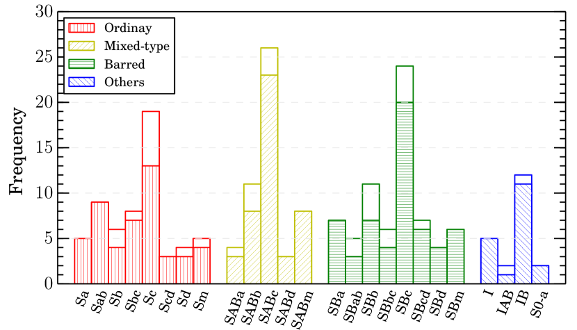
Figure 1: Frequency of galaxy morphological types of the ghasp sample according to the Hyperleda classification, separated in sections considering only ordinary spirals (59 galaxies), mixed types (52), barred (70), irregulars (19) and lenticulars (2).

3 Data reduction

3.1 Data from the ohp observatory

Broadband imaging for 128 galaxies in the R_c-band was obtained with the 1.2m telescope at the Observatoire de Haute-Provence (ohp), France, in several observation runs as presented in Table 2. The images have a field of view of 11.7’ x 11.7’, taken with a single CCD with 1024 x 1024 pixels, resulting in a pixel size of 0.685 arcsec^-1.

Table 2: List of observational runs in which the R_cphotometry of the ghasp galaxies was obtained at ohp.

Run	Dates	Number of
		Galaxies observed
(1)	2002 Mar 7th - Mar 13rd	29
(2)	2002 Oct 28th - Nov 10th	38
(3)	2003 Mar 8th - Mar 9th	17
(4)	2003 Mar 29th - Apr 6th	22
(5)	2003 Sep 22nd - Sep 28th	25
(6)	2003 Oct 21st - Oct 25th	6
(7)	2008 Jun 2nd - Jun 4th	11
(8)	2009 Oct 23rd	1
(9)	2010 Mar 19th - Mar 21st	16

Basic data reduction was performed with iraf tasks, including flat-field, bias subtraction and cosmic-ray cleaning. Images of the same galaxy are then aligned and combined for the cases with roughly the same smallest seeing FWHM, estimated from isolated field stars. Photometric stability check and zero point calibration was obtained by the observation of several standard stars from the catalog of Landolt (1992) in different times during the nights, considering the mean airmass correction coefficient of 0.145 for the R_c-band (Chevalier & Ilovaisky, 1991), and no colour term.

The determination of the sky level is the greatest source of uncertainty for surface brightness profiles and magnitudes (Courteau, 1996). For this purpose, we adopt the method of estimating the background by selecting sky “boxes” on the images, which are visually selected areas where the galaxy and stellar light contribution is minimal, and use those regions to calculate a smooth surface using the iraf package imsurfit with polynomials of order 2, which is subtracted from the original images. This process resulted in an homogeneous background for which the typical residual standard deviation is in the range 0.5-1% of the sky level.

We have modeled the Point Spread Function (PSF) of our images using the iraf psfmeasure task. We selected bright, unsaturated stars across the fields using the task daofind, and then modeled their light profiles using a circular Moffat function (Moffat, 1969), given by

$$\text{PSF}(r)=\frac{\beta-1}{\pi\alpha^{2}}\left[1+\left(\frac{r}{\alpha}\right)^{2}\right]^{-\beta}\text{,}$$ (1)

where the radial scale length $\alpha$ and the slope $\beta$ are free parameters, which can be related to the seeing by the relation FWHM$=2\alpha\sqrt{2^{1/\beta}-1}$ (see also Trujillo et al., 2001). This method has proved to be suitable in our case due to the presence of extended wings in the PSFs. Overall, the typical seeing of our observations is FWHM$\approx$3 arcsec, with the parameters $\alpha$, $\beta$ and FWHM having mean statistical uncertainties of 1.7%, 9% and 3% respectively.

3.2 Data from sdss

To increase the number of galaxies in our photometric sample in the R_c-band, we use sdss DR7 (Abazajian et al., 2009) archival data for 108 ghasp galaxies we found in the database and transformed sdss $ugriz$ data into R_cwith a multi-band scaling relation (more details in section 4.1). Among these 108 galaxies, 66 have also been observed in the OHP, thus 42 new ones are added to the final photometric sample. Calibrations and the PSF of the images are obtained directly from the data products of the survey. We performed a new sky determination for each image for consistency with the adopted method for R_cimages, and also because a few authors have pointed out errors in the sky determinations on images with bright galaxies in early sdss releases (e.g. Bernardi et al., 2007; Lauer et al., 2007; Lisker et al., 2007).

4 Data analysis

4.1 Surface photometry

We study the photometric properties of the sample using the traditional method of elliptical isophote fitting (Kent, 1984; Jedrzejewski, 1987). Surface brightness (SB) profiles of the galaxies were obtained using the iraf task ellipse, which provides a number of parameters that describe the light of the galaxy as a function of the semi-major axis (which we simply refer to as the radius, $r$), including the ellipticity ($\varepsilon$), position angle (PA) and the curve of growth, which quantifies the total apparent magnitude inside each isophote.

Masks for foreground and background objects were produced interactively in two steps. Firstly, most objects in the images were detected and masked out with SExtractor (Bertin and Arnouts, 1996). Other important sources not detected by the program, such as saturated stars and stars/galaxies superposed to the galaxies of interest were then masked during ellipse runs. Finally, we checked the results inspecting the residual image produced by subtracting an interpolated model of the galaxy produced with the task bmodel. This process was carried out several times for each galaxy until no bright sources were observed in the resulting subtracted images except for spiral arms and/or bars of the galaxy not masked on purpose.

The centre of each galaxy was defined in a first iteration of ellipse and later was set fixed for all other iterations. The position angle and ellipticity of the isophotes were usually set free to vary as a function of the radial distance, as usually done for late-type galaxy photometry (e.g. Balcells et al., 2003; MacArthur et al., 2003; McDonald, Courteau, & Tully, 2009), but in a few cases we were forced to fix the geometric parameters in part or in the whole galaxy in order to obtain convergence for the photometry. For the sdss data, we adopt this method in the r-band images, due to its relatively high signal-to-noise ratio in the $ugriz$ system, but we fix the position angles and ellipticities accordingly to the r-band parameters in the other pass bands in order to obtain consistent colours.

Uncertainties for the SB profiles include the isophote determination error given by ellipse, the photon counting statistics of the detector, and the sky level subtraction uncertainty, all added in quadrature. All profiles are corrected for the Galactic foreground extinction using the dust reddening maps of Schlegel et al. (1998), assuming a dust model with constant selective extinction of 3.1, and relative extinction for the different pass bands according to table 6 of Schlegel et al. (1998). However, we do not attempt for a correction of the SB profiles for the more uncertain problem of the galaxies’ internal extinction.

Finally, to obtain R_c-band SB profiles from sdss data, we use a slightly modified version of the relation derived by Jester et al. (2005), given by

$$\mu_{R}(r)=0.42\mu_{g}(r)-0.38\mu_{r}(r)+0.96\mu_{i}(r)-0.16\text{,}$$ (2)

where $\mu(r)$ represents the surface brightness profile at radius $r$ in the pass band indicated in the subscripts. The equation above was originally derived for stellar photometry, so we have tested its accuracy in surface photometry by the comparison of OHP SB profiles, obtained directly in the R_c-band, with profiles derived from the SDSS $ugriz$ bands using a sample of 54 galaxies for which the geometric parameters of both data sets are similar. The results are presented in Figure 2, which shows the difference of the profiles as a function of the OHP surface brightness profiles relative to the sky level, which varies in the OHP observations, from one galaxy observation to another. The red line shows the running RMS difference between the profiles, indicating that the error in the process of transforming between the photometric systems is of $\sim 0.08$ mag arcsec^-2 in the regions brighter than the sky level, $\sim 0.15$ mag arcsec^-2 for the regions down to two magnitudes fainter than the sky, and $\sim 0.4$ mag arcsec^-2 for the regions 5 magnitudes fainter than the sky level.

We present a sample of SB profiles for a variety of morphological types in Figure 3, including also the ellipticity and position angle variations. All surface brightness profiles are available in electronic format. In the next section, we detail other catalogued R_c-band photometric properties derived from SB profiles in this section.

Figure 2: Difference between R_csurface brightness profiles for OHP and SDSS data for 54 galaxies in common to both samples as a function of the OHP SB profile relative to the sky level. Profiles for the sdss galaxies are obtained using equation (2). Each blue line represents the difference in the surface brightness profiles of a single galaxy profile comparison. The dashed red lines indicates the running RMS difference between the profiles.

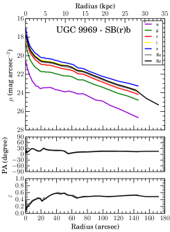
Figure 3: Examples of surface brightness profiles in the R_c-band, position angle and ellipticity profiles for six galaxies for which data are available both for the OHP and for the SDSS data sets. The surface brightness profiles are presented in different colours for each band according to the upper right labels, and uncertainties are not presented for the sake of clarity. The middle and lower panels of each galaxy show the position angle and ellipticity profiles respectively, with gray representing the r-band results and black representing the R_c-band geometry. All profiles are corrected for the Galactic foreground extinction according to the dust maps of Schlegel et al. (1998).

4.2 Integrated and isophotal photometry in the R_c-band

For the R_c-band SB profiles derived in this work, we obtained a number of properties of the galaxies which are of general interest by fixing a reference isophotal level. In the case of the R_c-band, the isophotal level of 23.5 mag arcsec${}^{\text{-2}}$ is usually used as reference, because it corresponds to an aperture similar to the B-band isophote of 25 mag arcsec${}^{\text{-2}}$. However, this level was reached for only 72% of our surface brightness profiles. Therefore, in order to provide a more complete catalogue for our sample, we also use the isophotal level of 22.5 mag arcsec${}^{\text{-2}}$ to provide parameters for 98% of the sample.

We measured the isophotal radius ($r_{\rm iso}$), position angle (PA_iso), ellipticity ($\varepsilon_{\rm iso}$) and apparent magnitude ($m_{\rm R,iso}$) directly from the SB profiles, with uncertainties estimated by Monte Carlo simulations of perturbations of the profile according to their uncertainties. Also, the inclination of the galaxies is estimated at a given isophotal level as (Tully & Fisher, 1988)

$$\cos i_{\rm iso}=\frac{(1-\varepsilon_{\rm iso})^{2}-q_{0}^{2}}{1^{2}-q_{0}^{2}}\mbox{,}$$ (3)

where $q_{0}=0.2$ is the intrinsic flattening of edge-on disks (e.g. Haynes & Giovanelli, 1984; Courteau, 1996).

We also measured the total (asymptotic) apparent magnitudes of the galaxies ($m_{\rm R,total}$), which were calculated by the extrapolation of the curve of growth of the SB profiles using a derivative method similar to Cairós et al. (2001). However, this method failed in cases of galaxies for which the curve of growth did not converge. In these cases, we used the last isophote total magnitude to estimate a lower limit to the total magnitude. Also using the curve of growth, we measured the effective radius of the galaxies ($r_{50}$), which is defined as the radius containing 50% of the total light of the galaxy. In the cases where we have not obtained a safe total magnitude, we then estimated the lower limits of the effective radius. Uncertainties in these parameters are also based on Monte Carlo simulations.

Table 3 presents a sample of the results for the isophotal level of 22.5 mag arcsec${}^{\text{-2}}$. The complete catalogue, and the catalogue for the isophotal level of 23.5 mag arcsec${}^{\text{-2}}$ are provided in the supplementary material.

Table 3: Isophotal and integrated photometric parameters in R_cband. The printed version contains only an abridged version of the table, and the remaining material is available online. (1) Galaxy name. (2) Data source. (3-7) Position angle, ellipticity, inclination, radius and apparent integrated magnitude at the isophote of 22.5 mag arcsec^-2. (8) Effective radius. (9) Total apparent magnitude.

Galaxy	Data	PA22.5	$\varepsilon_{22.5}$	$i_{22.5}$	$r_{22.5}$	$m_{\rm R,22.5}$	$r_{50}$	$m_{\rm R,total}$
		(arcsec)	(degree)	(degree)	(arcsec)	(mag)	(arcsec)	(mag)
(1)	(2)	(3)	(4)	(5)	(6)	(7)	(8)	(9)
UGC 89	OHP	$-27\pm 11$	$0.22\pm 0.03$	$40\pm 3$	$41\pm 2$	$11.60\pm 0.03$	$19\pm 5$	$11.4\pm 0.1$
UGC 94	OHP	$-84\pm 2$	$0.30\pm 0.02$	$46\pm 1$	$28\pm 1$	$13.12\pm 0.03$	$16\pm 7$	$12.7\pm 0.4$
IC 476	SDSS	$-79\pm 3$	$0.4\pm 0.1$	$52\pm 9$	$16\pm 2$	$14.7\pm 0.1$	$>10.0$	$<14.53$
UGC 508	OHP	$-61\pm 4$	$0.11\pm 0.05$	$28\pm 7$	$67\pm 1$	$11.17\pm 0.03$	$40\pm 1$	$10.91\pm 0.08$
UGC 528	OHP	$52\pm 2$	$0.03\pm 0.02$	$13\pm 3$	$65\pm 3$	$10.16\pm 0.01$	$21\pm 1$	$10.10\pm 0.04$
NGC 542	SDSS	$-34\pm 2$	$0.73\pm 0.01$	$79.1\pm 0.9$	$23\pm 2$	$14.39\pm 0.05$	$12\pm 6$	$14.2\pm 0.6$
UGC 763	OHP	$-75\pm 23$	$0.12\pm 0.02$	$29\pm 3$	$57\pm 4$	$11.61\pm 0.06$	$47\pm 5$	$11.1\pm 0.2$
UGC 763	SDSS	$-79\pm 35$	$0.12\pm 0.08$	$29\pm 10$	$56\pm 6$	$11.7\pm 0.1$	$>39.0$	$<11.46$
UGC 1013	OHP	$80\pm 2$	$0.62\pm 0.01$	$70.6\pm 0.7$	$53\pm 1$	$12.03\pm 0.01$	$27\pm 4$	$11.7\pm 0.1$
UGC 1013	SDSS	$80\pm 3$	$0.64\pm 0.01$	$72.2\pm 0.8$	$51\pm 5$	$12.17\pm 0.04$	$23\pm 3$	$11.9\pm 0.1$
…	…	…	…	…
UGC 12082	OHP	$18\pm 2$	$0.42\pm 0.01$	$56.1\pm 0.9$	$19\pm 3$	$15.0\pm 0.2$	$49\pm 23$	$12.8\pm 0.5$
UGC 12101	OHP	$-50\pm 2$	$0.53\pm 0.01$	$64.2\pm 0.8$	$51\pm 2$	$12.50\pm 0.03$	$29\pm 2$	$12.32\pm 0.09$
UGC 12101	SDSS	$-50\pm 3$	$0.52\pm 0.02$	$64\pm 1$	$49\pm 4$	$12.66\pm 0.06$	$28\pm 21$	$12.3\pm 0.9$
UGC 12212	OHP	$-80\pm 5$	$0.36\pm 0.02$	$52\pm 1$	$14\pm 1$	$15.8\pm 0.2$	$27\pm 26$	$14\pm 2$
UGC 12212	SDSS	$-71\pm 2$	$0.3\pm 0.01$	$46.8\pm 0.8$	$12\pm 5$	$15.9\pm 0.6$	$>16.0$	$<14.77$
UGC 12276	OHP	$-47\pm 6$	$0.23\pm 0.01$	$40.8\pm 0.9$	$30\pm 1$	$13.00\pm 0.03$	$19\pm 5$	$12.6\pm 0.2$
UGC 12276c	OHP	$82\pm 2$	$0.45\pm 0.01$	$58.3\pm 0.7$	$7\pm 1$	$17.0\pm 0.2$	$>5.0$	$<16.62$
UGC 12343	OHP	$38\pm 2$	$0.30\pm 0.03$	$47\pm 2$	$102\pm 1$	$10.33\pm 0.03$	$71\pm 9$	$10.2\pm 0.2$
UGC 12632	OHP	$22\pm 2$	$0.53\pm 0.05$	$64\pm 4$	$24\pm 5$	$14.8\pm 0.3$	$66\pm 59$	$13\pm 1$
UGC 12754	OHP	$-13\pm 3$	$0.29\pm 0.01$	$46\pm 1$	$89\pm 3$	$11.16\pm 0.03$	$47\pm 2$	$10.9\pm 0.1$

4.3 Multicomponent Decomposition

In our forthcoming work (Pineda et al. in preparation), we plan to study the kinematic properties of a subsample of ghasp galaxies with specific photometric properties depending on the relative importance of the disks in comparison with bulges and bars. In order to separate the SB brightness profiles into different structural components, we proceed to a multicomponent decomposition of the SB profiles.

For that purpose, we use a parametric profile fitting method which includes as many components as necessary to separate the photometric components – disks, bulges, bars, spiral arms, lens and nuclear sources. Ideally, one could use a complete 2D fitting to better describe the non axisymmetric components, like the bar, but the reliability of the 1D method to recover the structural parameters is comparable to 2D, at least for the disk component (MacArthur et al., 2003), and also allows the estimation of the integrated properties with good accuracy.

We have performed the decomposition in all R_c-band profiles in the ghasp OHP sample. We developed a Python routine which performs a weighted chi-square minimization between the data and a model using the Levenberg-Marquardt algorithm (see, eg. Press et al., 1992), using a PSF convolution of the models with a Moffat function (see section 3.1). The input model is set manually according to the observation of photometric features in the SB profile and the images of the galaxies. Also, the observation of the varying ellipticity and position angle as a function of the radius usually hinted for the different structural sub components of a galaxy. Figure 4 presents examples of structural decomposition of a sample of twelve galaxies, illustrating the variety of morphologies we have in our sample and the varied decomposition components we included. The structural parameters for all galaxies are listed in Table 4. In the next section, we give some details on the used parametrizations for the different components.

Table 4: Decomposition parameters for the ghasp sample in the R_cband obtained at the OHP observatory. The printed version contains only a sample of the table, and the remaining material is available online. (1) Galaxy name. (2-4) Parameters for the Sérsic function of bulges, bars and other components. (5) Visual classification of the components. (6-10) Parameters for the disks according to the broken exponential function. (11) Classification of the disks regarding to the type of breaks, according to the scheme of Erwin et al. (2008, see text for details). (12) Magnitude of the central point source.

	Sérsic				Diskg						PS
Galaxy	$\mu_{b}$	$r_{e}$	$n$	type	$\mu_{d}$	$h_{i}$	$h_{o}$	$r_{b}$	$\alpha$	Type	$m_{\rm ps}$
	(mag arcsec-2)	(arcsec)				(mag arcsec-2)	(arcsec)	(arcsec)	(arcsec)		(mag)
(1)	(2)	(3)	(4)	(5)	(6)	(7)	(8)	(9)	(10)	(11)	(12)
UGC 89	$16.7\pm 0.1$	$2.3\pm 0.1$	$1.0\pm 0.1$	bulge	$21.5\pm 1.0$	$35\pm 25$	—	—	—	Type I	—
	$20.3\pm 0.2$	$19\pm 1$	$0.2\pm 0.1$	bar	—	—	—	—	—		—
	$23\pm 1$	$29\pm 5$	$0.11\pm 0.07$	bar	—	—	—	—	—		—
UGC 94	$18.7\pm 0.3$	$0.8\pm 0.3$	$1.6\pm 0.3$	bulge	$20.3\pm 0.1$	$14.0\pm 0.8$	—	—	—	Type I	—
	$20.79\pm 0.09$	$8.3\pm 0.4$	$0.14\pm 0.09$	bar	—	—	—	—	—		—
UGC 508	$18.6\pm 0.2$	$3.4\pm 0.1$	$2.65\pm 0.04$	bulge	$19.60\pm 0.04$	$26.2\pm 0.2$	—	—	—	Type I	—
	$23.69\pm 0.08$	$20.2\pm 0.3$	$0.05\pm 0.05$	bar	—	—	—	—	—		—
	$21.19\pm 0.06$	$7.6\pm 0.3$	$0.22\pm 0.02$	bar	—	—	—	—	—		—
UGC 528	$19.0\pm 0.2$	$5.4\pm 0.6$	$2.7\pm 0.3$	bulge	$18.6\pm 0.2$	$19\pm 2$	—	—	—	Type I	—
	$19.8\pm 0.2$	$13.1\pm 0.8$	$0.1\pm 0.2$	arms	—	—	—	—	—		—
	$20.3\pm 0.4$	$22\pm 1$	$0.15\pm 0.09$	arms	—	—	—	—	—		—
UGC 763	$28.0\pm 0.3$	$311\pm 183$	$5.3\pm 0.3$	bulge	$19.99\pm 0.06$	$25\pm 2$	—	—	—	Type I	—
	$23\pm 2$	$18\pm 9$	$0.05\pm 0.06$	bar	—	—	—	—	—		—
…	…	…	…	…	…	…	…	…	…	…	…
UGC 12276	$21.1\pm 0.1$	$5.4\pm 0.2$	$2.56\pm 0.01$	bulge	$20.24\pm 0.09$	$14.0\pm 0.1$	$7.0\pm 0.3$	$45.0\pm 0.1$	$1.0\pm 0.2$	Type II	—
	$27.36\pm 0.05$	$0.1\pm 0.1$	$6.59\pm 0.04$	bar	—	—	—	—	—		—
UGC 12276c	$22.74\pm 0.09$	$0.0\pm 0.1$	$2.99\pm 0.08$	bulge	$20.60\pm 0.09$	$3.6\pm 0.2$	—	—	—	Type I	—
UGC 12343	$20.9\pm 0.4$	$12\pm 3$	$2.9\pm 0.3$	bulge	$19.2\pm 0.1$	$30\pm 3$	—	—	—	Type I	—
	$21.7\pm 0.4$	$56\pm 3$	$0.2\pm 0.1$	bar	—	—	—	—	—		—
UGC 12632	$23.1\pm 0.2$	$2.9\pm 0.6$	$0.05\pm 0.08$	nucleus	$22.1\pm 0.1$	$58\pm 4$	—	—	—	Type I	—
	$23.4\pm 0.2$	$9.8\pm 0.4$	$0.10\pm 0.02$	bulge	—	—	—	—	—		—
UGC 12754	$20.36\pm 0.07$	$11.8\pm 0.4$	$0.43\pm 0.04$	bar	$20.6\pm 0.2$	$56\pm 7$	—	—	—	Type I	$15.7\pm 0.2$
	$22.4\pm 0.4$	$24\pm 1$	$0.05\pm 0.06$	bar	—	—	—	—	—		—

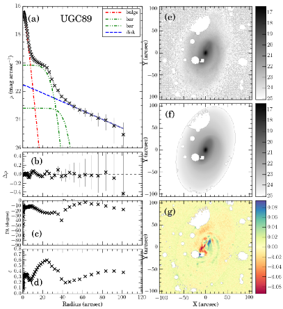
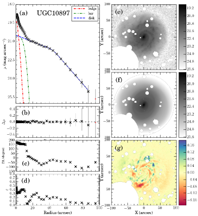
Figure 4: Examples of structural decomposition for two galaxies of the GHASP sample in the R_c-band, UGC 89 and UGC 10897. For each galaxy, we present seven panels, containing (a) surface brightness profiles and their decomposition components, (b) fitting residuals, (c) position angle profile, (d) ellipticity profile, (e) R_c-band image, (f) ellipse model and (g) residual sigma image.

4.3.1 Disks

Since early works of Patterson (1940) and de Vaucouleurs (1958), the intensity profile of disks have been mostly described by a simple exponential law,

$$I_{d}(r)=I_{0}\exp\left(-\frac{r}{h}\right),$$ (4)

where $I_{0}$ is the central ($r=0$) intensity of the disk and $h$ is the disk scale length. Usually, we refer to the central intensity in terms of surface brightness using the relation $\mu_{0}=-2.5\log I_{0}$. For the case of exponential disks, the total apparent magnitude is given by

$$m_{\text{disk}}=-2.5\log\left(2\pi I_{0}h^{2}\frac{b}{a}\right)\mbox{,}$$ (5)

where $b/a=1-\varepsilon$ is the minor-to-major axis ratio of the galaxy.

However, deviations from a simple exponential disk were already noticed by Freeman (1970), specially in the form of truncations or breaks in the inner profiles of galaxies. Later, van der Kruit & Searle (1982) also noticed breaks at large radii of disks, and more recently deviations at very low surface brightness have been observed, including upward bends (e.g. Erwin et al., 2005).

Based on these observations, Erwin et al. (2008) proposed a reviewed classification of disks in three categories: Type I, simple disks well described by exponential disks; Type II, disks with downward truncations; and Type III, disks with upward bends. A local census of disk properties performed by Pohlen & Trujillo (2006) of late-type galaxies (Sb-Sm) estimated the fraction of Type I galaxies to be only 10%, while 60% are classified as Type II and 30% are Type III according to this new classification scheme. Therefore, an updated profile for the disks is here adopted whenever breaks are clearly observed, by using broken exponential profiles, given by (Erwin et al., 2008)

$$I_{d}(r)=SI_{0}\exp\left(-\frac{r}{h_{i}}\right)\cdot\left\{1+\exp\left[\alpha(r-r_{b})\right]\right\}^{\frac{1}{\alpha}(\frac{1}{h_{i}}-\frac{1}{h_{o}})}\mbox{,}$$ (6)

where $I_{0}$ is the central intensity of the disk, $h_{i}$ and $h_{o}$ are the inner and outer disk scale length respectively, $r_{b}$ is the break radius, $\alpha$ is the sharpness of the disk transition between the inner and outer region (where low $\alpha$ means a smooth transition from the inner to the outer disk and high $\alpha$ means an abrupt transition), and $S$ is a scaling factor given by

$$S=\left[1+\exp(-\alpha r_{b})\right]^{-\frac{1}{\alpha}(\frac{1}{h_{i}}-\frac{1}{h_{o}})}\mbox{.}$$ (7)

For the broken disks in our sample, the total luminosities were calculated numerically, given that a solution by the integration of equation (6) is beyond the scope of this work.

In Table 4, we include a classification of the disks according to our observations. However, it is important to notice that breaks may occur at different radial distances, with different physical interpretations: inner breaks ($\mu_{r}\sim 23$ mag arcsec^-2) may be related to star formation, while outer breaks ($\mu_{r}\sim 27$ mag arcsec^-2) may indicate a real drop in the stellar mass density (Martín-Navarro et al., 2012). Therefore, our classifications are restricted to the mean limiting surface brightness of 24.5 mag arcsec^-2.

4.3.2 Other components

Apart from the disk, several other components are observed, including bulges, bars, arms, rings and lenses. We included those components in the decomposition using a Sérsic function (Sersic, 1968), given by

$$I_{b}(r)=I_{e}\exp\left(-b_{n}\left[\left(\frac{r}{r_{e}}\right)^{1/n}-1\right]\right),$$ (8)

where $r_{e}$ is the effective scale of the component (for which 50% of the light is within $r_{e}$), $I_{e}$ is the intensity at the effective radius, and $n$ is the Sérsic index. The term $b_{n}$ is not a free parameter, but a function of the Sérsic index due to the parametrization of the function at the effective radius instead of at the centre. In our calculations, we adopted the expressions for $b_{n}$ presented in the Appendix [A1] of MacArthur et al. (2003). In a first order approximation, $b_{n}\approx 2n-0.33$, although the error may be considerable for $n<0.5$. For simplification, we also rescale the effective intensity to surface brightness using the expression $\mu_{e}=-2.5\log I_{e}$. In the case of equation (8), the total magnitude is given by (Ciotti, 1991; MacArthur et al., 2003)

$$m_{\rm sersic}=-2.5\log\left(\frac{2\pi I_{e}r_{e}^{2}\mathrm{e}^{b_{n}}n\Gamma(2n)}{b_{n}^{2n}}\frac{b}{a}\right)\mbox{,}$$ (9)

where $\Gamma(x)$ is the complete gamma function of a variable $x$. The Sérsic profile is a generalization of other commonly used profile functions, such as the exponential for $n=1$, a Gaussian for $n=\frac{1}{2}$ and a de Vaucouleurs’s profile (de Vaucouleurs, 1948) for $n=4$. Moreover, the Sérsic index can also be used as an indicator of the kind of component that is being observed. For example, in the optical and near-infrared wavelengths, Fisher and Drory (2010) have shown that $n\lesssim 2$ may indicate a pseudobulge, whereas $n\gtrsim 2$ may indicate a classic bulge for the spheroidal components. Besides, bars have typically $n\sim 0.7$ (Gadotti, 2011). In the Table 4, where the decomposition results are presented, we include a classification of the Sérsic function components according to the visual inspection of images and profiles, such as bulges, bars, lenses and spiral arms.

In 35 galaxies, a nuclear source is also detected, which may be related to different physical processes, such as an active nucleus or a stellar concentration. We have tested two approaches for parametrizing these components, using either a Sérsic component or a single delta function with a peak at $r=0$. In 12 cases, the former approach resulted in a better description of the nucleus, because they have slightly larger FWHM than that of the modelled PSF and/or because of the different shape of the nuclear source compared to a star. These components are described as nucleus in tables 4 in the column 5. For 23 galaxies, however, the later approach of using a delta function resulted in a better description of the nucleus in these cases. This delta function has only one free parameter, the magnitude of the source ($m_{\rm ps}$), and its profile is of a field star which is described as a Moffat function. These point source magnitudes are included in the last row of Table 4.

5 Photometric Internal Consistency and Literature Comparison

In this section we make a series of tests on our photometric results to verify their consistency and to compare them with similar results in the literature. We have already made an internal consistency check of our SB profiles in Figure 2, where we observed that the SB profiles from sdss data are similar to those observed with direct measurements in the R_c-band. Our SB profiles can also be compared with those derived for twelve galaxies in common with de Jong and van der Kruit (1994) in the R_c-band, as shown in Figure 5, where black and red lines show the difference between our and the literature data for the ohp and sdss data sets respectively. To make a proper comparison, we have fixed the position angle and the ellipticity of the galaxies to mimic the method of those authors instead of using free position angle and ellipticity as in section 4.1. We also limited the comparison to regions greater than the seeing of our images.

The most deviant case is UGC 4256, but the internal consistency of our results for two different data sets indicates a possible systematic offset in the data of de Jong and van der Kruit (1994) for this galaxy. The deviation in the outer region of UGC 508 can be explained by the limited field of view in the images of de Jong and van der Kruit (1994) which cuts part of the galaxy. In this case, it is also possible to see a large variation of the isophotes fainter than 21 mag arcsec² within the observations of de Jong and van der Kruit. Finally, the problematic case of UGC 10445 for the ohp data can be explained by the relatively short exposure time for this object, including only one image, which affects the accuracy of the sky subtraction. Apart from these remarks, the overall picture is a good agreement with de Jong and van der Kruit (1994), which is in turn in agreement with several other authors in the literature.

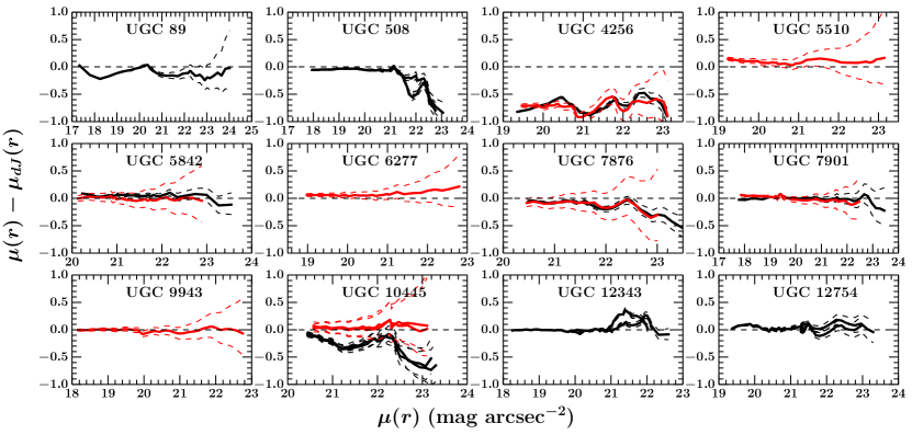
Figure 5: Difference between the surface brightness as function of the isophotal level for 12 galaxies profiles in common with de Jong and van der Kruit (1994) in the R_c-band. The solid black (red) lines represent the data from the ohp (sdss), while the dashed lines are the profile errors. Multiple profiles of galaxies in de Jong and van der Kruit (1994) are shown in different lines. Dashed lines represent the errors in our profiles.

In Figure 6, we show the internal consistency of the isophotal and integrated photometric parameters derived from the SB profiles by the comparison of the results obtained with the ohp and sdss data sets, including position angle, ellipticity, integrated magnitude and radius at the isophote of 22.5 mag/arcsec² and also effective radius and total magnitude. We also display the mean residual difference ($<\Delta>$) and its standard deviation ($\sigma(\Delta)$) for each parameter, resulting in compatible measurements in both data sets within one standard deviation.

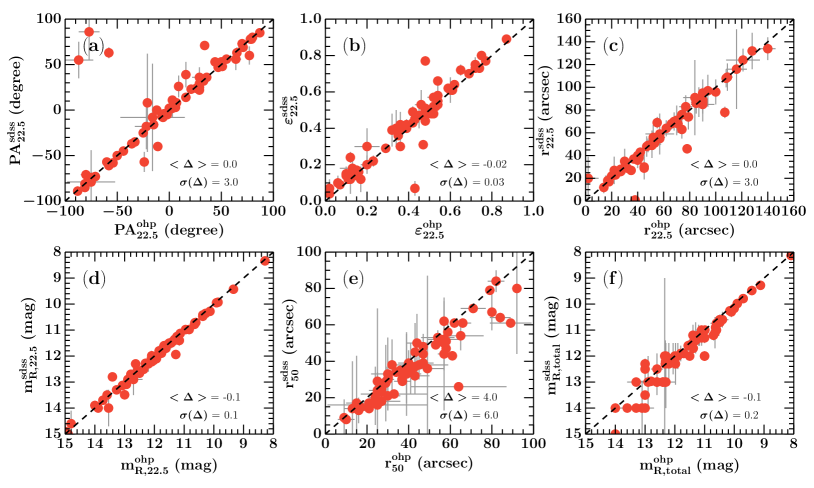
Figure 6: Comparison of photometric properties derived for the 66 galaxies in common between the ohp and sdss datasets. The parameter $\Delta$ represents the difference between the parameters in the two data sets, with its the mean value ($<\Delta>$) and its standard deviation ($\sigma(\Delta)$) shown in the bottom of each panel. Parameters are displayed as the following: (a) isophotal position angle; (b) isophotal ellipticity; (c) isophotal radius; (d) isophotal apparent magnitude; (e) effective radius; (f) total apparent magnitude. The horizontal and vertical axes display the results for the ohp and sdss datasets respectively, and the dashed line represents the ideal equality between datasets.

In Figure 7 we compare our total magnitudes with data in the literature. There are just a few works in the literature for which total magnitudes are measured in the R_c-band, so we also include in the figure measurements in similar filters in the literature without any additional correction or extrapolation, which are displayed as gray symbols, including Tully et al. (1996), James et al. (2004), Cabrera-Lavers & Garzón (2004), Taylor et al. (2005), Doyle et al. (2005), Hernández-Toledo et al. (2007), Thomas et al. (2008), Hernández-Toledo & Ortega-Esbrí (2008), Matthews & Uson (2008) and Kriwattanawong et al. (2011). However, specially relevant is the comparison with proper R_cmagnitudes, which we highlight in Figure 7 using coloured symbols for the works of Heraudeau & Simien (1996), Gil de Paz et al. (2003), Kassin, de Jong, & Pogge (2006) and Amorín et al. (2007). The number of overlapping galaxies with R_c-band data is scarce, only 12 galaxies, but those are in good agreement with most previous works, specially with the more recent survey of Kassin, de Jong, & Pogge (2006).

Figure 7: Comparison of total apparent magnitudes with the literature. Coloured symbols indicate the comparisons with data in the R_c-band, including the works of Heraudeau & Simien (1996), Gil de Paz et al. (2003), Kassin, de Jong, & Pogge (2006) and Amorín et al. (2007). Gray symbols indicate the comparisons with magnitudes in pass bands similar to R_cwith our magnitudes both for the sdss (circles) and ohp (crosses) samples. This later data include magnitudes from Hickson et al. (1989), Tully et al. (1996), James et al. (2004), Cabrera-Lavers & Garzón (2004), Taylor et al. (2005), Doyle et al. (2005), Hernández-Toledo et al. (2007), Noordermeer and van der Hulst (2007), Thomas et al. (2008), Hernández-Toledo & Ortega-Esbrí (2008), Matthews & Uson (2008) and Kriwattanawong et al. (2011). The dashed line represents equality between measurements.

In the top panel of Figure 8, we compare our isophotal radius with the results of James et al. (2004). As the reference isophotal levels are different, there is a systematic offset in the isophotal radius in the sense that results from our work are systematically smaller than those from James et al., but still there is a good correspondence between the two datasets. In the bottom panel of Figure 8, we show that the ellipticities are also well correlated, as expected, because at both reference isophotal levels the disk is the dominant component in the light of the galaxy, and has a simple geometry that does not vary drastically between these pass bands. Finally, in figure 9, we compare the isophotal position angles and inclinations with the results from the H$\alpha$ map analysis of Epinat et al. 2008, which demonstrate that our analysis produces results that are similar even to other tracers of the galaxy shape such as the gas.

Figure 8: Comparison of our isophotal radius (above) and ellipticity (below) with those derived by James et al. (2004). Filled (hollow) points represent data from OHP (SDSS), and the dashed lines represent the equality between measurements.

Figure 9: Comparison of our isophotal position angles (above) and inclinations (below) with those derived from the H$\alpha$ velocity fields of Epinat et al. 2008. Filled (hollow) points represent data from OHP (SDSS), and the dashed line represents the equality between measurements.

6 Scaling relations

Scaling relations contain important information about the physical processes regarding galaxy formation and evolution, and impose important constraints to models that attempt to describe such objects (Courteau et al., 2007). In this section, we derive the most significant scaling relation involving luminosities, sizes and rotation curve velocity for each of the two most basic structural components of the galaxy, the bulge and the disk, and also for the whole galaxy. In section 6.1, we show how we correct the sizes and luminosities for the effects of distance, inclination and dust attenuation, and in section 6.2 we show how we estimate the scaling relations. In section 6.3 we present the main results and in section 6.4 we explore the Tully-Fisher relation in greater detail.

6.1 Correction for the effects of inclination and distances

We use all galaxies in table 4 with a bulge component according to our classification in the decomposition. Disk apparent magnitudes ($m_{\text{disk}}$) are calculated using equation (5) or by numerical integration in the case of broken profiles for the disks, while bulge luminosities ($m_{\text{bulge}}$) are calculated using equation (8). The absolute magnitudes of these components are then obtained using the equations

$$M_{\text{disk}}=m_{\text{disk}}-d_{1}-d_{2}(1-\cos i)^{d_{3}}-5\log D-25\mbox{,}$$ (10)

$$M_{\text{bulge}}=m_{\text{bulge}}-b_{1}-b_{2}(1-\cos i)^{b_{3}}-5\log D-25\mbox{,}$$ (11)

where the internal extinction coefficients $b_{1}=0.60$, $b_{2}=1.33$, $b_{3}=1.75$, $d_{1}=0.15$, $d_{2}=1.09$ and $d_{3}=2.82$ are obtained by linear interpolation from Table 1 of Driver et al. (2008) for the R_c-band ($\lambda=647$nm), $D$ is the distance in Mpc according to Epinat et al. (2008), and the inclination $i$ is taken from the gas velocity field analysis in Epinat et al. (2008), if available, or from the isophotal analysis otherwise. Individual distance errors are rarely available, and we adopt a value of $25\%$ for all objects.

The total luminosity of each galaxy is estimated by its total magnitude according to the analysis of the curve of growth of the SB profiles (see section 4.2). In this case, we obtain the absolute magnitude of the galaxies ($M_{\rm R,total}$) from the apparent total magnitudes ($m_{\rm R,total}$) using the expression

$$M_{\rm R,total}=m_{\rm R,total}-A_{i}(R)-5\log D-25\text{,}$$ (12)

where $A_{i}(R)$ is the internal extinction correction given by Tully et al. (1998)

$$A_{i}(R)=\log(b/a)\times\left\{1.15+1.88\left(\log 2V_{\text{max}}-2.5\right)\right\}\text{.}$$ (13)

Here $b/a$ is again the minor-to-major axis ratio and $V_{\text{max}}$ is the maximum velocity of the H$\alpha$ rotation curve derived from the velocity field analysis from Epinat et al. (2008).

We compare these luminosities with the physical sizes of each component, using the scale length of disks ($h$), or the inner disk length in the cases of broken disks, the effective radius of the bulge ($r_{e}$) and the effective radius of the galaxy ($r_{50}$). We do not attempt to correct the sizes of the components for extinction, and we only rescale the sizes according to the distance. Finally, we use the velocity $V_{\text{max}}$ as in Epinat et al. (2008) as our dynamical tracer, excluding galaxies for which the flat part of the rotation curve was not reached in the velocity field analysis of the H$\alpha$ observations.

6.2 Fitting method

We assessed the statistical significance of pairs of luminosities, sizes and velocities using the Spearman’s rank correlation coefficient $r$, which is a measurement of the strength of the correlation of two variables, and the associated p-value $p$, which indicates the probability of obtaining a result at least as extreme as the one obtained from a random distribution, both indicated in the boxes at the top of each panel. For 18 cases, we obtained correlations with $p<0.1$%, for which we calculated scaling laws considering the direct and inverse cases. The relations, displayed in the form of dashed lines in Figure 10, were calculated as in the following. We consider a linear relation in the form of

$$y_{i}=\alpha x_{i}+\beta\mbox{,}$$ (14)

where each galaxy is represented by the index $i$, $\alpha$ is the slope of the relation and $\beta$ is the zero point. We then performed a $\chi^{2}$ minimization considering the measurement uncertainties in both variables, considering also an intrinsic scatter, $\varepsilon_{0}$, for the relation (see Tremaine et al., 2002), using the relation

$$\chi^{2}_{\nu}=\frac{1}{N-2}\sum_{i=1}^{N}\frac{\left(y_{i}-\beta-\alpha x_{i}\right)^{2}}{\varepsilon_{yi}^{2}+\alpha^{2}\varepsilon_{xi}^{2}+\varepsilon_{0}^{2}}\mbox{,}$$ (15)

where $N$ is the number of galaxies of the sample, $\nu=N-2$ is the number of degrees of freedom, $\varepsilon_{xi}$ and $\varepsilon_{yi}$ are the parameter uncertainties. The presence of the variables in both the numerator and in the denominator of relation (15) makes the equation non-linear, and most common methods of minimization, such as the Levenberg-Marquardt algorithm (Press et al., 1992), may have problems to obtain convergence. To obtain stable solutions, we used the interactive method described by Bedregal et al. (2006), which consists in solving equation (15) for a fixed value of $\varepsilon_{0}$, and then update $\varepsilon_{0}$ by multiplying for $\chi^{2}_{\nu}$ elevated to a power of $2/3$, until obtaining $\chi^{2}_{\nu}=1$. This method failed in only two cases, as show in table 5, because either the dispersion is too low and $\chi^{2}<1$ or if the dispersion was too high. The uncertainties for the coefficients were estimated using the bootstrapping method.

6.3 Results

Figure 10 shows the resulting relations among luminosities, sizes and velocities for 62 galaxies selected in the previous section. We adopt different colouring for the panels above and below the diagonal according to the strength of the bar and to the morphological classification respectively. However, we could not study these correlations in subsamples due to the low statistics after dividing the data in those classes, and our quantitative results are all related to the complete photometric sample. The summary of the scaling laws is shown in table 5, where we sort the relations by decreasing Spearman’s coefficients.

Figure 10: R_c-band correlations between luminosities and sizes of bulges ($M_{\rm bulge}$, $\log r_{e}$), disks ($M_{\rm disk}$ and $\log h$) and the galaxy luminosities ($M_{\rm R,total}$), sizes ($r_{50}$) and maximum velocity of the rotation curve ($V_{\rm max}$). Panels above the diagonal display colours of galaxies according to the colour map in the bottom right of the figure, which divide galaxies according to the presence of bars following the morphological classification. Panels below the diagonal display colours according to the colourmap in the bottom left of the figure, classifying galaxies according to their numerical type in the de Vaucouleurs’s classification. The Spearman’s rank correlation coefficient ($r_{s}$) and the p-value of the relation are presented in the box on top of each panel. For relations with significance greater than 3$\sigma$, we include a dashed black line to indicate the best fit linear regression, whose coefficients are presented in Table 5. The diagonal panels display the distributions of parameters as histograms.

Table 5: Scaling relations with statistical significance above 3$\sigma$ for the luminosities, sizes and velocity of the galaxies and its two basic subcomponents, bulges and disks, ranked by decreasing Spearman’s rank coefficients ($r_{s}$). The first column indicates the identification of the relation. The second column indicates the variables involved in the relation, as well as the correlation coefficients and their p-values. The third column indicates the direct and inverse relations. The fourth column shows the intrinsic scatter of the relation.

ID	Parameters	Relation	$\varepsilon_{0}$
(1)	(2)	(3)	(4)
(a)	$M_{\mbox{R,total}}$-$M_{\mbox{disk}}$	$M_{\mbox{disk}}=(0.98\pm 0.03)M_{\mbox{R,total}}+(-0.6\pm 0.7)$	—
	$|r|=0.96$, $p=3\cdot 10^{-34}$	$M_{\mbox{R,total}}=(1.02\pm 0.04)M_{\mbox{disk}}+(0.6\pm 0.8)$	—
(b)	$\log V_{\mbox{max}}$-$M_{\mbox{R,total}}$	$M_{\mbox{R,total}}=(-8.0\pm 0.7)\log V_{\mbox{max}}+(-3\pm 1)$	$0.37\pm 0.05$
	$|r|=0.88$, $p=6\cdot 10^{-21}$	$\log V_{\mbox{max}}=(-0.12\pm 0.01)M_{\mbox{R,total}}+(-0.2\pm 0.2)$	$0.04\pm 0.01$
(c)	$\log V_{\mbox{max}}$-$M_{\mbox{disk}}$	$M_{\mbox{disk}}=(-7.1\pm 0.8)\log V_{\mbox{max}}+(-5\pm 2)$	$0.31\pm 0.07$
	$|r|=0.85$, $p=2\cdot 10^{-18}$	$\log V_{\mbox{max}}=(-0.13\pm 0.01)M_{\mbox{disk}}+(-0.6\pm 0.3)$	$0.04\pm 0.01$
(d)	$\log r_{50}$-$\log h$	$\log h=(0.88\pm 0.07)\log r_{50}+(0.00\pm 0.04)$	$0.132\pm 0.003$
	$|r|=0.85$, $p=4\cdot 10^{-18}$	$\log r_{50}=(0.93\pm 0.06)\log h+(0.11\pm 0.03)$	$0.135\pm 0.004$
(e)	$\log r_{50}$-$M_{\mbox{disk}}$	$M_{\mbox{disk}}=(-4.7\pm 0.3)\log r_{50}+(-18.1\pm 0.2)$	$0.61\pm 0.03$
	$|r|=0.83$, $p=9\cdot 10^{-17}$	$\log r_{50}=(-0.18\pm 0.02)M_{\mbox{disk}}+(-3.2\pm 0.3)$	$0.12\pm 0.01$
(f)	$M_{\mbox{R,total}}$-$M_{\mbox{bulge}}$	$M_{\mbox{bulge}}=(1.1\pm 0.1)M_{\mbox{R,total}}+(5\pm 3)$	$1.11\pm 0.02$
	$|r|=0.82$, $p=2\cdot 10^{-16}$	$M_{\mbox{R,total}}=(0.65\pm 0.06)M_{\mbox{bulge}}+(-9\pm 1)$	$0.84\pm 0.02$
(g)	$\log r_{50}$-$M_{\mbox{R,total}}$	$M_{\mbox{R,total}}=(-4.4\pm 0.5)\log r_{50}+(-18.1\pm 0.3)$	$0.88\pm 0.02$
	$|r|=0.78$, $p=9\cdot 10^{-14}$	$\log r_{50}=(-0.16\pm 0.02)M_{\mbox{R,total}}+(-2.7\pm 0.3)$	$0.167\pm 0.005$
(h)	$\log V_{\mbox{max}}$-$M_{\mbox{bulge}}$	$M_{\mbox{bulge}}=(-9\pm 1)\log V_{\mbox{max}}+(2\pm 2)$	$1.17\pm 0.07$
	$|r|=0.76$, $p=7\cdot 10^{-13}$	$\log V_{\mbox{max}}=(-0.08\pm 0.01)M_{\mbox{bulge}}+(0.8\pm 0.2)$	$0.107\pm 0.007$
(i)	$\log h$-$M_{\mbox{disk}}$	$M_{\mbox{disk}}=(-4.3\pm 0.4)\log h+(-18.6\pm 0.2)$	$0.86\pm 0.02$
	$|r|=0.72$, $p=3\cdot 10^{-11}$	$\log h=(-0.16\pm 0.02)M_{\mbox{disk}}+(-2.8\pm 0.4)$	$0.165\pm 0.006$
(j)	$M_{\mbox{R,total}}$-$\log h$	$\log h=(-0.15\pm 0.02)M_{\mbox{R,total}}+(-2.5\pm 0.3)$	$0.181\pm 0.004$
	$|r|=0.72$, $p=5\cdot 10^{-11}$	$M_{\mbox{R,total}}=(-4.3\pm 0.6)\log h+(-18.4\pm 0.3)$	$0.98\pm 0.01$
(k)	$M_{\mbox{disk}}$-$M_{\mbox{bulge}}$	$M_{\mbox{bulge}}=(1.0\pm 0.1)M_{\mbox{disk}}+(3.0\pm 3.0)$	$1.42\pm 0.03$
	$|r|=0.69$, $p=4\cdot 10^{-10}$	$M_{\mbox{disk}}=(0.55\pm 0.09)M_{\mbox{bulge}}+(-11.0\pm 2.0)$	$1.03\pm 0.02$
(l)	$\log r_{e}$-$M_{\mbox{bulge}}$	$M_{\mbox{bulge}}=(-4.1\pm 0.6)\log r_{e}+(-19.6\pm 0.1)$	$1.41\pm 0.02$
	$|r|=0.67$, $p=3\cdot 10^{-09}$	$\log r_{e}=(-0.14\pm 0.02)M_{\mbox{bulge}}+(-2.9\pm 0.3)$	$0.262\pm 0.004$
(m)	$\log V_{\mbox{max}}$-$\log r_{50}$	$\log r_{50}=(1.1\pm 0.2)\log V_{\mbox{max}}+(-1.8\pm 0.4)$	$0.204\pm 0.007$
	$|r|=0.65$, $p=1\cdot 10^{-08}$	$\log V_{\mbox{max}}=(0.5\pm 0.1)\log r_{50}+(1.95\pm 0.06)$	$0.134\pm 0.005$
(n)	$\log V_{\mbox{max}}$-$\log h$	$\log h=(1.0\pm 0.1)\log V_{\mbox{max}}+(-1.7\pm 0.3)$	$0.205\pm 0.008$
	$|r|=0.63$, $p=3\cdot 10^{-08}$	$\log V_{\mbox{max}}=(0.46\pm 0.06)\log h+(1.98\pm 0.04)$	$0.141\pm 0.004$
(o)	$\log h$-$M_{\mbox{bulge}}$	$M_{\mbox{bulge}}=(-4.6\pm 0.8)\log h+(-16.3\pm 0.4)$	$1.66\pm 0.02$
	$|r|=0.60$, $p=3\cdot 10^{-07}$	$\log h=(-0.09\pm 0.01)M_{\mbox{bulge}}+(-1.1\pm 0.3)$	$0.231\pm 0.002$
(p)	$\log r_{50}$-$M_{\mbox{bulge}}$	$M_{\mbox{bulge}}=(-3.7\pm 0.8)\log r_{50}+(-16.6\pm 0.5)$	$1.83\pm 0.02$
	$|r|=0.53$, $p=1\cdot 10^{-05}$	$\log r_{50}=(-0.08\pm 0.02)M_{\mbox{bulge}}+(-0.8\pm 0.4)$	$0.260\pm 0.004$
(q)	$\log h$-$\log r_{e}$	$\log r_{e}=(0.8\pm 0.3)\log h+(-0.6\pm 0.2)$	$0.41\pm 0.01$
	$|r|=0.48$, $p=9\cdot 10^{-05}$	$\log h=(0.3\pm 0.2)\log r_{e}+(0.62\pm 0.03)$	$0.28\pm 0.01$
(r)	$\log r_{50}$-$\log r_{e}$	$\log r_{e}=(0.6\pm 0.2)\log r_{50}+(-0.5\pm 0.1)$	$0.362\pm 0.002$
	$|r|=0.41$, $p=1\cdot 10^{-03}$	$\log r_{50}=(0.3\pm 0.1)\log r_{e}+(0.68\pm 0.02)$	$0.275\pm 0.003$

All equations in table 5 can be used as a way of obtaining approximate physical parameters for one given measurement as well as for constraining models of galaxy formation at the current cosmic time. Out of the 21 pairs of parameters, we observe that only three combinations have relatively low correlation coefficients. This indicates that most of the spiral galaxy properties are somehow linked. Although there are many possible properties that shape galaxies, such as different mass, angular momentum, and despite secular evolution effects, such as those which may form bars, there is still a great similarity among spirals which is still to be explained. Also, this large number of correlations restrict the interpretation of the correlations individually, and certainly a comprehensible interpretation will be possible only with a more complete model of galaxy evolution (see Shen et al., 2010). Nevertheless, we are going to briefly discuss a few of the scaling laws that have been observed here and previously in the literature, with the exception of the Tully-Fisher relation (Tully and Fisher, 1977), which we address with greater detail in 6.4.

The relation (q) between the sizes of bulges and disks was obtained previously by other authors (Courteau et al., 1996; Aguerri et al., 2005) and may have important clues for galaxy formation scenarios. Courteau et al. (1996) argue that disks should have been formed earlier than bulges and, therefore, the properties of the bulges are linked to their host disks. Due to the relatively low Sérsic indices of the bulges, these are indeed likely to be pseudobulges (Fisher and Drory, 2008), which are formed by secular evolution of the disks and, therefore, correlations among these parameters naturally arise in a scenario of secular evolution, disfavoring scenarios of decoupled size relation such as bulges formed by mergers. We have found that the median value of $r_{e}/h$ is 0.14 considering all galaxies, which is in agreement to the values in the literature (for instance, Laurikainen et al., 2010).

The luminosity of bulge is also of importance to understand its origin. Bulge luminosities and sizes are expected to correlate, as already indicated in equation (9), $L_{\mbox{bulge}}\propto r_{e}^{2}$, and indeed there is a strong correlation as shown in equation (l). Moreover, the bulge luminosity is correlated to all other measured properties of the disks, to the whole galaxy and also to the rotation velocity. Therefore, the properties of the bulges we observe in late-type galaxies of the local universe are probably the result of secular evolution. Interestingly, the bulge luminosity is also correlated with the supermassive black hole masses (Kormendy & Richstone, 1995), illustrating the important role of the bulges to understand the processes of galaxy formation yet to be fully understood.

Another parameter that correlates strongly with almost all the others is the luminosity of the galaxy, as shown in equations (a), (b), (f), (g) and (j). The importance of the total luminosity, also observed by Courteau et al. (2007), may indicate that the baryonic portion of the galaxy has a pivotal role in the appearance of galaxies: it is connected with the gravitational potential through the velocity, but has a more direct link with the size (or shape) of the galaxy.

Other photometric relations well documented in the literature include the relation (k) between bulge and disk luminosities (Laurikainen et al., 2010), and (f) which relates bulge and total luminosities (Carollo et al., 2007). The rotation velocity of the galaxies is usually studied in comparison with integrated photometry, such as given in relation (b), the Tully-Fisher relation, and the size-velocity relation (m) also studied by Courteau et al. (2007). However, here we show that the rotation velocity also strongly correlate with the luminosity and size of the disk component, as shown in relations (c) and (n), which is expected because the disk is responsible for the majority of the light of the galaxy. Interestingly, however, the luminosity of the bulge also correlates with the rotation velocity, as shown in relation (h), indicating that the bulge properties have a dynamical link with the galaxy that hosts it.

6.4 Tully-Fisher relation

The Tully-Fisher relation (hereafter TF relation, Tully and Fisher, 1977) is the most important scaling relation for disk galaxies, and it has been used for several purposes including distance determinations and, historically, as a way of measuring the Hubble constant. The TF relation relates the maximum velocity of the rotation curve, $V_{\text{max}}$ with the total magnitude of the galaxies in the form of a power law. The TF relation has already been measured in the ghasp sample previously by Torres-Flores et al. (2011) in the near-infrared bands H and K, so here we add to those results the optical R_c-band. We adopt the following parametrization

$$M_{\lambda}=\alpha_{\lambda}\cdot\log\left(\frac{V_{\rm max}}{\text{km/s}}\right)+\beta_{\lambda}\text{,}$$ (16)

where $M_{\lambda}$ is the absolute total magnitude in the passband $\lambda$, $V_{\rm max}$ is the maximum velocity of the rotation curve, $\alpha_{\lambda}$ and $\beta_{\lambda}$ are the slope and the zero point of the TF relation. Both the slope and the zero point of the Tully Fisher relation are of importance because they may be used either as constraints or as tests for models of galaxy formation and evolution.

To produce a suitable sample for this specific relation, we select the galaxies according to the following criteria. We remove galaxies with inclinations greater than $75$^∘due to their high internal extinction, and also galaxies with inclinations smaller than $20$^∘because of their higher uncertainty in the determination of the rotation curve velocity. We also exclude galaxies with recession velocities lower than 3000 km s^-1 due to possible peculiar velocities affecting the Hubble flow, except for the cases where more accurate distance indicators were used, such as Cepheids and red-giant branch distances. Finally, as we are only dealing with H$\alpha$ velocity fields, we use the analysis of Epinat et al. (2008) to exclude from the sample galaxies for which the maximum rotation velocity is not achieved according to their classification of the maps. We use our two absolute magnitude estimators, the asymptotic ($M_{\rm R,total}$) and the isophotal ($M_{\rm R,23.5}$) as the probe of the galaxy luminosity, resulting in samples with 80 and 72 galaxies respectively. Most galaxies of ghasp sample are not part of clusters of galaxies, so we consider that our TF relation is basically probing the field environment, although the expected difference of the TF relation in different environments is mild (De Rijcke et al., 2007; Mocz et al., 2012).

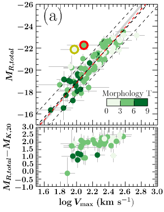
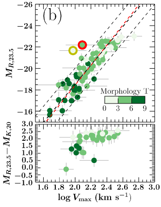
Figure 11: Tully-Fisher relation for the R_c-band for ghasp galaxies considering (a) the total asymptotic magnitude, $M_{\rm R,total}$, and (b) the isophotal total magnitude inside the isophote of 23.5 mag arcsec^-2. The gray line in panel (a) indicates the results from Sakai et al. (2000). In the top panel of each figure, the black dashed line indicates the direct TF relation results and the best fit $\pm 1\sigma_{\beta}$, while the red dashed line indicates the inverse TF relation results. The bottom panels indicates the colour of the galaxies using the K band total magnitudes used for the TF relation in Torres-Flores et al. (2011) inside the isophote of 20 mag arcsec^-2. The colour of each galaxy reflects the colourbar scale in the upper panels, separating objects according to their numerical morphology. The two objects highlighted with a halo are NGC 12276 (yellow) and NGC 4256 (red), which for different reasons are offset to the TF relation (see text for details).

The TF relation in the R_c-band is shown in Figure 11. To calculate the regression coefficients, we have used the $\chi^{2}$ minimization of equation (15) as described in section 6.3. Also, the so-called inverse Tully-Fisher relation (Schechter, 1980) coefficients are calculated as follows. We calculated the coefficients $\alpha^{\prime}$ and $\beta^{\prime}$ by interchanging the variables $x_{i}\rightleftarrows y_{i}$ in equation (14), and then calculated the inverse TF relation using the relations $\alpha=1/\alpha^{\prime}$ and $\beta=-\beta^{\prime}/\alpha^{\prime}$. The summary of the results for the TF relation and the inverse TF relations is presented in Table 6.

Table 6: Regression coefficients for the R_c-band Tully-Fisher relation using the total asymptotic magnitude and the total isophotal magnitude including 80 and 72 galaxies respectively.

Relation	$\alpha_{R}$	$\beta_{R}$	$\varepsilon_{0}$
Total asymptotic magnitude
TF	$-8.1\pm 0.5$	$-3.0\pm 1.0$	$0.28\pm 0.07$
Inverse TF	$-8.4\pm 0.7$	$-2.0\pm 2.0$	$0.28\pm 0.08$
Total isophotal magnitude
TF	$-8.9\pm 0.6$	$-1.0\pm 1.0$	$0.33\pm 0.06$
Inverse TF	$-9.3\pm 0.7$	$0.0\pm 2.0$	$0.34\pm 0.08$

The TF relation is not just an important tool for measuring distances of galaxies, but it is also crucial to highlight processes of galaxy evolution, for instance, by comparing the TF relation of different morphological types. Spiral galaxies have a single TF relation, but lenticular and elliptical galaxies have TF relations which run approximately parallel when compared to spirals (Bedregal et al., 2006; De Rijcke et al., 2007). We observe that the TF relation of spirals in the R_cband is well defined for almost all galaxies, with only two exceptions that are worth discussing. NGC 12276, marked in the figure 11 with a yellow halo, does not seem to have any special feature to be offset from the TF relation, so one possibility to explain its position is that the distance to the galaxy is not accurate. We have used the value of 78.8 Mpc from Epinat et al. (2008) for consistency with the previous works, which is the expected value according to the systematic velocity using the Hubble flow. However, Pedreros & Madore (1981) have estimated the distance to this galaxy of 40 Mpc using the ring size, which implies in a difference of $\approx$1.5 magnitudes that is enough to bring the galaxy much closer to the TF relation. The galaxy with a red halo in figure 11, NGC 4256, has a peculiar morphology of a single arm and an asymmetric rotation curve, which may be the cause to move the galaxy off the TF relation defined by relatively more relaxed spirals. In this case, star formation may have been triggered recently as a response to a gravitational field, resulting in a relatively luminous object compared to the TF relation.

The slope and the zero point of the R_c-band TF relation in our work are in agreement with those previously derived the literature. Tully and Pierce (2000), for instance, determined the slope and zero point for a sample of 115 galaxies in four nearby clusters with velocities derived from HI line widths, and by not considering errors in both variables nor the intrinsic scatter of the relation, they have found $\alpha_{R}=-7.65$ and $\beta_{R}=-4.3$, which is consistent with our results within 2 sigmas. On the other hand, Verheijen (2001) has derived the TF relation for the Ursa Major cluster using the inverse relation without intrinsic scatter, and fixing the uncertainties in 0.05 mag for the magnitudes and 5% in the velocities. In this framework, they found slopes ranging from -7.1 to -9, and zero points ranging from -3.15 to 2.81 for their various samples, which is similar to our inverse TF relation parameters.

The TF relation in the infrared pass bands is important because these wavelengths are reliable tracers of the stellar masses. Torres-Flores et al. (2011) have used the ghasp sample to derive the TF relation in the H and K bands using 2MASS survey data (Skrutskie et al., 2006) as well as stellar and baryonic TF relations, and using a method similar to ours, they have obtained slopes of $\alpha_{H}=-10.84\pm 0.61$ and $\alpha_{K}=-11.07\pm 0.63$ and zero points of $\beta_{H}=1.97\pm 1.36$ and $\beta_{k}=2.27\pm 1.39$ for the H and K bands respectively. As expected, the R_c-band slope is greater than the slope in the near-infrared band (e.g. Verheijen, 2001). However, one important feature observed in the infrared is a break in the TF relation for galaxies with $\log V_{max}\lesssim 2.2$, in the sense that galaxies below this velocity are under luminous related to the expected TF relation for bright galaxies. This break in the TF relation is not noticed in the R_c-band. This difference in the shapes of the near-infrared and optical TF at the low-mass regime can be understood if one inspects the bottom panels of Figure 11, which show the optical to near-infrared colours of the galaxies as a function of the maximum rotation velocities. These panels show a flat colour distribution except for the galaxies with $V_{\rm max}\lesssim 125$ km s^-1, indicating different mass-to-light ratios these galaxies. These low mass systems are bluer than more massive galaxies, indicating younger objects that may have been forming stars recently, and this effect fortuitously compensates for the difference in the stellar mass to light ratios, causing the differences in the shapes of the near-infrared and optical TFs at low masses.

7 Summary and Conclusion

This study provided photometrically calibrated surface brightness profiles of ghasp galaxies, with 170 profiles in the R_c-band and 108 in the sdss bands u,g,r,i and z. From these data, we derived R_c-band integrated photometric parameters, presented in Table 3, which are consistent with other works in the literature. All these results are public and will be available in digital format at the Fabry Perot repository in http://cesam.lam.fr/fabryperot.

We perform multi component structural decompositions in the R_c-band, presented in Table 4, with the goal of separating the disk component from bulges, bars, lenses and nuclear sources, as a preparation to our forthcoming paper on the kinematic decomposition of ghasp velocity fields, which will be compared with the photometric work.

Finally, we have applied new photometric data to observe bulges, disks and global scaling relations among luminosities, sizes and velocities in the R_c-band. We derived expressions for 18 scaling relations, which may be used to constrain models of galaxy formation and evolution. In particular, we studied the Tully Fisher relation using velocities derived solely from H$\alpha$ maps from ghasp. We have obtained slopes and zero points that are consistent with previous findings in the literature in the R_c-band for cluster galaxies, reinforcing the idea that the Tully Fisher relation is basically a relation between the total stellar content and the gravitational potential, which is barely affected by the environment and the presence of photometric substructures.

References

- Abazajian et al. (2009) Abazajian K. N., Adelman-McCarthy J. K., Agüeros M. A., Allam S. S., Allende Prieto C., An D., Anderson K. S. J., Anderson S. F., Annis J., Bahcall N. A., et al., ApJS, 2009, vol.182, p. 543
- Aguerri et al. (2005) Aguerri, J. A. L., Elias-Rosa, N., Corsini, E. M., & Muñoz-Tuñón, C. 2005, A&A, 434, 109
- van Albada et al. (1985) van Albada T. S., Bahcall J. N., Begeman K., Sancisi R., 1985, ApJ, 295, 305
- van Albada & Sancisi (1986) van Albada, T. S., & Sancisi, R. 1986, Royal Society of London Philosophical Transactions Series A, 320, 447
- Amorín et al. (2007) Amorín, R. O., Muñoz-Tuñón, C., Aguerri, J. A. L., Cairós, L. M., & Caon, N. 2007, A&A, 467, 541
- Balcells et al. (2003) Balcells M., Graham A. W., Domínguez-Palmero L., Peletier R. F., 2003, ApJ, 582, L79
- Bedregal et al. (2006) Bedregal, A. G., Aragón-Salamanca, A., & Merrifield, M. R. 2006, MNRAS, 373, 1125
- Bernardi et al. (2007) Bernardi, M., Hyde, J. B., Sheth, R. K., Miller, C. J., Nichol, R. C., AJ, 133, 1741B
- Bertin and Arnouts (1996) Bertin, E., Arnouts, S., A&AS, 117, 393
- Cabrera-Lavers & Garzón (2004) Cabrera-Lavers, A., & Garzón, F. 2004, AJ, 127, 1386
- Cairós et al. (2001) Cairós L. M., Caon N., Vílchez J. M., González-Pérez J. N., Muñoz-Tuñón C., ApJS, 2001, vol. 136, p. 393
- Carollo et al. (2007) Carollo, C. M., Scarlata, C., Stiavelli, M., Wyse, R. F. G., & Mayer, L. 2007, ApJ, 658, 960
- Chevalier & Ilovaisky (1991) Chevalier C., Ilovaisky S. A., 1991, A&AS, 90, 225
- Ciotti (1991) Ciotti, L. 1991, A&A, 249, 99
- Courteau (1996) Courteau S., 1996, ApJS, 103, 363
- Courteau et al. (1996) Courteau, S., de Jong, R. S., & Broeils, A. H. 1996, ApJL, 457, L73
- Courteau et al. (2007) Courteau, S., Dutton, A. A., van den Bosch, F. C., et al. 2007, ApJ, 671, 203
- De Rijcke et al. (2007) De Rijcke, S., Zeilinger, W. W., Hau, G. K. T., Prugniel, P., & Dejonghe, H. 2007, ApJ, 659, 1172
- Driver et al. (2008) Driver, S. P., Popescu, C. C., Tuffs, R. J., et al. 2008, ApJL, 678, L101
- Doyle et al. (2005) Doyle, M. T., Drinkwater, M. J., Rohde, D. J., et al. 2005, MNRAS, 361, 34
- Dutton et al. (2005) Dutton A. A., Courteau S., de Jong R., Carignan C., 2005, ApJ, 619, 218
- Epinat, Amram & Marcelin (2008) Epinat B., Amram P., Marcelin M., 2008, MNRAS, 390, 466E
- Epinat et al. (2008) Epinat B., Amram P., Marcelin M., Balkowski C., Daigle O., Hernandez O., Chemin L., Carignan C., Gach J.-L., Balard P., 2008, MNRAS, 388, 500E
- Epinat et al. (2010) Epinat B., Amram P., Balkowski C., Marcelin M., 2010, MNRAS, 401, 2113
- Erwin et al. (2005) Erwin, P., Beckman, J. E., & Pohlen, M. 2005, ApJL, 626, L81
- Erwin et al. (2008) Erwin, P., Pohlen, M., & Beckman, J. E. 2008, AJ, 135, 20
- Fisher and Drory (2008) Fisher D. B., Drory N., AJ, 2008, vol. 136, p. 773
- Fisher and Drory (2010) Fisher D. B., Drory N., ApJ, 2010, vol. 716, p. 942
- Freeman (1970) Freeman K. C., ApJ, 1970, vol. 160, p. 811
- Gadotti (2011) Gadotti D. A., 2011, MNRAS, 415, 3308
- Garrido et al. (2002) Garrido O., Marcelin M., Amram P., Boulesteix J., 2002, A&A, 387, 821
- Garrido et al. (2003) Garrido O., Marcelin M., Amram P., Boissin O., 2003, A&A, 399, 51
- Garrido, Marcelin, & Amram (2004) Garrido O., Marcelin M., Amram P., 2004, MNRAS, 349, 225
- Garrido et al. (2005) Garrido O., Marcelin M., Amram P., Balkowski C., Gach J. L., Boulesteix J., 2005, MNRAS, 362, 127
- Gil de Paz et al. (2003) Gil de Paz, A., Madore, B. F., & Pevunova, O. 2003, ApJS, 147, 29
- Haynes & Giovanelli (1984) Haynes M. P., Giovanelli R., 1984, AJ, 89, 758
- Heraudeau & Simien (1996) Heraudeau, P., & Simien, F. 1996, A&AS, 118, 111
- Hernández-Toledo et al. (2007) Hernández-Toledo, H. M., Zendejas-Domínguez, J., & Avila-Reese, V. 2007, AJ, 134, 2286
- Hernández-Toledo & Ortega-Esbrí (2008) Hernández-Toledo, H. M., & Ortega-Esbrí, S. 2008, A&A, 487, 485
- Hickson et al. (1989) Hickson, P., Kindl, E., & Auman, J. R. 1989, ApJS, 70, 687
- Huchra (1977) Huchra, J. P. 1977, ApJS, 35, 171
- van der Hulst, van Albada, & Sancisi (2001) van der Hulst J. M., van Albada T. S., Sancisi R., 2001, ASPC, 240, 451
- James et al. (2004) James, P. A., Shane, N. S., Beckman, J. E., et al. 2004, A&A, 414, 23
- Jedrzejewski (1987) Jedrzejewski R. I., MNRAS, 1987, vol. 226, p. 747
- Jester et al. (2005) Jester S., Schneider D. P., Richards G. T., Green R. F., Schmidt M., Hall P. B., Strauss M. A., Vanden Berk D. E., Stoughton C., Gunn J. E., Brinkmann J., Kent S. M., Smith J. A., Tucker D. L., Yanny B., AJ, 2005, vol. 130, p. 873I c
- de Jong and van der Kruit (1994) de Jong R. S., van der Kruit P. C., A&AS, 1994, vol. 106, p. 451
- Kassin, de Jong, & Pogge (2006) Kassin S. A., de Jong R. S., Pogge R. W., 2006, ApJS, 162, 80
- Kassin, de Jong, & Weiner (2006) Kassin S. A., de Jong R. S., Weiner B. J., 2006, ApJ, 643, 804
- Kent (1984) Kent, S. M. 1984, ApJS, 56, 105
- Kent (1986) Kent S. M., 1986, AJ, 91, 1301
- Kormendy & Richstone (1995) Kormendy, J., & Richstone, D. 1995, ARA&A, 33, 581
- Kriwattanawong et al. (2011) Kriwattanawong, W., Moss, C., James, P. A., & Carter, D. 2011, A&A, 527, A101
- van der Kruit & Searle (1982) van der Kruit, P. C., & Searle, L. 1982, A&A, 110, 61
- Landolt (1992) Landolt A. U., 1992, AJ, 104, 340L
- Lauer et al. (2007) Lauer, T. R., Faber, S. M., Richstone, D., Gebhardt, K., Tremaine, S., Postman, M., Dressler, A., Aller, M. C., Filippenko, A. V., Green, R., Ho, L. C., Kormendy, J., Magorrian, J., Pinkney, J., ApJ, 662, 808L
- Laurikainen et al. (2010) Laurikainen, E., Salo, H., Buta, R., Knapen, J. H., & Comerón, S. 2010, MNRAS, 405, 1089
- Lisker et al. (2007) Lisker, T., Grebel, E. K., Binggeli, B., Glatt, K., 2007, ApJ, 660, 1186L
- MacArthur et al. (2003) MacArthur L. A., Courteau S., Holtzman J. A., ApJ, 2003, vol. 582, p. 689
- Martín-Navarro et al. (2012) Martín-Navarro I., et al., 2012, MNRAS, 427, 110
- Matthews & Uson (2008) Matthews, L. D., & Uson, J. M. 2008, AJ, 135, 291
- McDonald, Courteau, & Tully (2009) McDonald M., Courteau S., Tully R. B., 2009, MNRAS, 394, 2022
- Mocz et al. (2012) Mocz, P., Green, A., Malacari, M., & Glazebrook, K. 2012, MNRAS, 425, 296
- Moffat (1969) Moffat A. F. J., 1969, A&A, 3, 455
- Noordermeer and van der Hulst (2007) Noordermeer E., van der Hulst J. M., MNRAS, 2007, vol. 376, p. 1480
- Patterson (1940) Patterson, F. S. 1940, Harvard College Observatory Bulletin, 914, 9
- Pedreros & Madore (1981) Pedreros, M., & Madore, B. F. 1981, ApJS, 45, 541
- Pohlen & Trujillo (2006) Pohlen, M., & Trujillo, I. 2006, A&A, 454, 759
- Press et al. (1992) Press, W. H., Teukolsky, S. A., Vetterling, W. T., & Flannery, B. P. 1992, Cambridge: University Press, —c1992, 2nd ed.,
- De Rijcke et al. (2007) De Rijcke, S., Zeilinger, W. W., Hau, G. K. T., Prugniel, P., & Dejonghe, H. 2007, ApJ, 659, 1172
- Rubin, Thonnard, & Ford (1978) Rubin V. C., Thonnard N., Ford W. K., Jr., 1978, ApJ, 225, L107
- Schechter (1980) Schechter, P. L. 1980, AJ, 85, 801
- Sakai et al. (2000) Sakai, S., Mould, J. R., Hughes, S. M. G., et al. 2000, ApJ, 529, 698
- Schlegel et al. (1998) Schlegel D. J., Finkbeiner D. P., Davis M., ApJ, 1998, vol. 500, p. 525
- Sersic (1968) Sersic, J. L. 1968, Cordoba, Argentina: Observatorio Astronomico, 1968
- Shen et al. (2010) Shen, J., Rich, R. M., Kormendy, J., et al. 2010, ApJL, 720, L72
- Skrutskie et al. (2006) Skrutskie, M. F., Cutri, R. M., Stiening, R., et al. 2006, AJ, 131, 1163
- Spano et al. (2008) Spano M., Marcelin M., Amram P., Carignan C., Epinat B., Hernandez O., 2008, MNRAS, 383, 297
- Stoughton et al. (2002) Stoughton C., et al., 2002, AJ, 123, 485
- Taylor et al. (2005) Taylor, V. A., Jansen, R. A., Windhorst, R. A., Odewahn, S. C., & Hibbard, J. E. 2005, ApJ, 630, 784
- Thomas et al. (2008) Thomas, C. F., Moss, C., James, P. A., et al. 2008, A&A, 486, 755
- Torres-Flores et al. (2011) Torres-Flores S., Epinat B., Amram P., Plana H., Mendes de Oliveira C., 2011, MNRAS, 416, 1936
- Tremaine et al. (2002) Tremaine, S., Gebhardt, K., Bender, R., et al. 2002, ApJ, 574, 740
- Trujillo et al. (2001) Trujillo, I., Aguerri, J. A. L., Cepa, J., & Gutiérrez, C. M. 2001, MNRAS, 328, 977
- Tully & Fisher (1988) Tully, R. B., & Fisher, J. R. 1988, Catalog of Nearby Galaxies, by R. Brent Tully and J. Richard Fisher, pp. 224. ISBN 0521352991. Cambridge, UK: Cambridge University Press, April 1988.,
- Tully and Fisher (1977) Tully R. B., Fisher J. R., A&A, 1977, vol. 54, p. 661
- Tully et al. (1996) Tully, R. B., Verheijen, M. A. W., Pierce, M. J., Huang, J.-S., & Wainscoat, R. J. 1996, AJ, 112, 2471
- Tully et al. (1998) Tully, R. B., Pierce, M. J., Huang, J.-S., et al. 1998, AJ, 115, 2264
- Tully and Pierce (2000) Tully R. B., Pierce M. J., ApJ, 2000, vol. 533, p. 744
- de Vaucouleurs (1948) de Vaucouleurs G., 1948, AnAp, 11, 247
- de Vaucouleurs (1958) de Vaucouleurs, G. 1958, ApJ, 128, 465
- Verheijen (2001) Verheijen M. A. W., 2001, ApJ, 563, 694
- Zwicky (1937) Zwicky F., 1937, ApJ, 86, 217