Preconditioned low-rank Riemannian optimization for
linear systems with tensor product structure

Abstract

The numerical solution of partial differential equations on high-dimensional domains gives rise to computationally challenging linear systems. When using standard discretization techniques, the size of the linear system grows exponentially with the number of dimensions, making the use of classic iterative solvers infeasible. During the last few years, low-rank tensor approaches have been developed that allow to mitigate this curse of dimensionality by exploiting the underlying structure of the linear operator. In this work, we focus on tensors represented in the Tucker and tensor train formats. We propose two preconditioned gradient methods on the corresponding low-rank tensor manifolds: A Riemannian version of the preconditioned Richardson method as well as an approximate Newton scheme based on the Riemannian Hessian. For the latter, considerable attention is given to the efficient solution of the resulting Newton equation. In numerical experiments, we compare the efficiency of our Riemannian algorithms with other established tensor-based approaches such as a truncated preconditioned Richardson method and the alternating linear scheme. The results show that our approximate Riemannian Newton scheme is significantly faster in cases when the application of the linear operator is expensive.

Keywords: Tensors, Tensor Train, Matrix Product States, Riemannian Optimization, Low Rank, High Dimensionality

Mathematics Subject Classifications (2000): 65F10, 15A69, 65K05, 58C05

1 Introduction

This work is concerned with the approximate solution of large-scale linear systems $Ax=f$ with $A\in\mathbb{R}^{n\times n}$. In certain applications, such as the structured discretization of $d$-dimensional partial differential equations (PDEs), the size of the linear system naturally decomposes as $n=n_{1}n_{2}\cdots n_{d}$ with $n_{\mu}\in\mathbb{N}$ for $\mu=1,\ldots,d$. This allows us to view $Ax=f$ as a tensor equation

$$\mathcal{A}\mathbf{X}=\mathbf{F},$$ (1)

where $\mathbf{F},\mathbf{X}\in\mathbb{R}^{n_{1}\times n_{2}\times\cdots\times n_{d}}$ are tensors of order $d$ and $\mathcal{A}$ is a linear operator on $\mathbb{R}^{n_{1}\times n_{2}\times\cdots\times n_{d}}$.

The tensor equations considered in this paper admit a decomposition of the form

$$\mathcal{A}=\mathcal{L}+\mathcal{V},$$ (2)

where $\mathcal{L}$ is a Laplace-like operator with the matrix representation

$$L=I_{n_{d}}\otimes\cdots\otimes I_{n_{2}}\otimes L_{1}+I_{n_{d}}\otimes\cdots\otimes I_{n_{3}}\otimes L_{2}\otimes I_{n_{1}}+\cdots+L_{d}\otimes I_{n_{d-1}}\otimes\cdots\otimes I_{1},$$ (3)

with matrices $L_{\mu}\in\mathbb{R}^{n_{\mu}\times n_{\mu}}$ and identity matrices $I_{n_{\mu}}$. The term $\mathcal{V}$ is dominated by $\mathcal{L}$ in the sense that $\mathcal{L}$ is assumed to be a good preconditioner for $\mathcal{A}$. Equations of this form arise, for example, from the discretization of the Schrödinger Hamiltonian [41], for which $\mathcal{L}$ and $\mathcal{V}$ correspond to the discretization of the kinetic and the potential energy terms, respectively. In this application, $\mathcal{A}$ (and thus also $L_{\mu}$) is symmetric positive definite. In the following, we restrict ourselves to this case, although some of the developments can, in principle, be generalized to indefinite and nonsymmetric matrices.

Assuming $\mathcal{A}$ to be symmetric positive definite allows us to reformulate (1) as an optimization problem

$$\min_{{\mathbf{X}}\in\mathbb{R}^{n_{1}\times\cdots\times n_{d}}}\;\frac{1}{2}\langle\mathbf{X},\mathcal{A}\mathbf{X}\rangle-\langle\mathbf{X},\mathbf{F}\rangle$$ (4)

It is well-known that the above problem is equivalent to minimizing the $\mathcal{A}$-induced norm of the error $\|\mathbf{X}-\mathcal{A}^{-1}\mathbf{F}\|_{\mathcal{A}}$. Neither (1) nor (4) are computationally tractable for larger values of $d$. During the last decade, low-rank tensor techniques have been developed that aim at dealing with this curse of dimensionality by approximating ${\bf F}$ and ${\bf X}$ in a compressed format; see [18, 20] for overviews. One approach consists of restricting (4) to a subset $\mathcal{M}\subset\mathbb{R}^{n_{1}\times n_{2}\times\cdots\times n_{d}}$ of compressed tensors:

$$\min_{{\mathbf{X}}\in\mathcal{M}}\;f(\mathbf{X}):=\frac{1}{2}\langle\mathbf{X},\mathcal{A}\mathbf{X}\rangle-\langle\mathbf{X},\mathbf{F}\rangle.$$ (5)

Examples for $\mathcal{M}$ include the Tucker format [57, 31], the tensor train (TT) format [50], the matrix product states (MPS) format [4] or the hierarchical Tucker format [17, 22]. Assuming that the corresponding ranks are fixed, $\mathcal{M}$ is a smooth embedded submanifold of $\mathbb{R}^{n_{1}\times n_{2}\times\cdots\times n_{d}}$ for each of these formats [25, 58, 59, 23]. This property does not hold for the CP format, which we will therefore not consider.

When $\mathcal{M}$ is a manifold, Riemannian optimization techniques [1] can be used to address (5). In a related context, first-order methods, such as Riemannian steepest descent and nonlinear CG, have been successfully applied to matrix completion [9, 43, 47, 61] and tensor completion [11, 34, 51, 55].

Similar to Euclidean optimization, the condition number of the Riemannian Hessian of the objective function is instrumental in predicting the performance of first-order optimization algorithms on manifolds; see, e.g., [42, Thm. 2] and [1, Thm. 4.5.6]. As will be evident from (28) in §4.1, an ill-conditioned operator $\mathcal{A}$ can be expected to yield an ill-conditioned Riemannian Hessian. As this is the case for the applications we consider, any naive first-order method will be prohibitively slow and noncompetitive with existing methods.

For Euclidean optimization, it is well known that preconditioning or, equivalently, adapting the underlying metric can be used to address the slow convergence of such first-order methods. Combining steepest descent with the Hessian as a (variable) preconditioner yields the Newton method with (local) second order convergence [46, Sec. 1.3.1]. To overcome the high computational cost associated with Newton’s method, several approximate Newton methods exist that use cheaper second-order models. For example, Gauss–Newton is a particularly popular approximation when solving non-linear least-squares problems. For Riemannian optimization, the connection between preconditioning and adapting the metric is less immediate and we explore both directions to speed up first-order methods. On the one hand, we will consider a rather ad hoc way to precondition the Riemannian gradient direction. On the other hand, we will consider an approximate Newton method that can be interpreted as a constrained Gauss–Newton method. This requires setting up and solving linear systems with the Riemannian Hessian or an approximation thereof. In [62], it was shown that neglecting curvature terms in the Riemannian Hessian leads to an efficient low-rank solver for Lyapunov matrix equations. We will extend these developments to more general equations with tensors approximated in the Tucker and the TT formats.

Riemannian optimization is by no means the only sensible approach to finding low-rank tensor approximations to the solution of the linear system (1). For linear operators only involving the Laplace-like operator (3), exponential sum approximations [16, 21] and tensorized Krylov subspace methods [35] are effective and allow for a thorough convergence analysis. For more general equations, a straightforward approach is to apply standard iterative methods, such as the Richardson iteration or the CG method, to (1) and represent all iterates in the low-rank tensor format; see [6, 13, 27, 29, 36] for examples. One critical issue in this approach is to strike a balance between maintaining convergence and avoiding excessive intermediate rank growth of the iterates. Only recently, this has been analyzed in more detail [5]. A very different approach consists of applying alternating optimization techniques to the constrained optimization problem (5). Such methods have originated in quantum physics, most notably the so called DMRG method to address eigenvalue problems in the context of strongly correlated quantum lattice systems, see [53] for an overview. The ideas of DMRG and related methods have been extended to linear systems in the numerical analysis community in [14, 15, 24, 49] and are generally referred to as alternating linear schemes (ALS). While such methods often exhibit fast convergence, especially for operators of the form (2), their global convergence properties are poorly understood. Even the existing local convergence results for ALS [52, 59] offer little intuition on the convergence rate. The efficient implementation of ALS for low-rank tensor formats can be a challenge. In the presence of larger ranks, the (dense) subproblems that need to be solved in every step of ALS are large and tend to be ill-conditioned. In [33, 37], this issue has been addressed by combining an iterative solver with a preconditioner tailored to the subproblem. The design of such a preconditioner is by no means simple, even the knowledge of an effective preconditioner for the full-space problem (1) is generally not sufficient. So far, the only known effective preconditioners are based on exponential sum approximations for operators with Laplace-like structure (3), which is inherited by the subproblems.

Compared to existing approaches, the preconditioned low-rank Riemannian optimization methods proposed in this paper have a number of advantages. Due to imposing the manifold constraint, the issue of rank growth is completely avoided. Our methods have a global nature, all components of the low-rank tensor format are improved at once and hence the stagnation typically observed during ALS sweeps is avoided. Moreover, we completely avoid the need for solving subproblems very accurately. One of our methods can make use of preconditioners for the full-space problem (1), while for the other methods preconditioners are implicitly obtained from approximating the Riemannian Hessian. A disadvantage shared with existing methods, our method strongly relies on the decomposition (2) of the operator to construct effective preconditioners.

In passing, we mention that there is another notion of preconditioning for Riemannian optimization on low-rank matrix manifold, see, e.g., [44, 45, 47]. These techniques address the ill-conditioning of the manifold parametrization, an aspect that is not related and relevant to our developments, as we do not directly work with the parametrization.

The rest of this paper is structured as follows. In Section 2, we briefly review the Tucker and TT tensor formats and the structure of the corresponding manifolds. Then, in Section 3, a Riemannian variant of the preconditioned Richardson method is introduced. In Section 4, we incorporate second-order information using an approximation of the Riemannian Hessian of the cost function and solving the corresponding Newton equation. Finally, numerical experiments comparing the proposed algorithms with existing approaches are presented in Section 5.

2 Manifolds of low-rank tensors

In this section, we discuss two different representations for tensors $\mathbf{X}\in\mathbb{R}^{n_{1}\times n_{2}\times\cdots\times n_{d}}$, namely the Tucker and tensor train/matrix product states (TT/MPS) formats, along with their associated notions of low-rank structure and their geometry. We will only mention the main results here and refer to the articles by Kolda and Bader [31] and by Oseledets [50] for more details. More elaborate discussions on the manifold structure and computational efficiency considerations can be found in [30, 34] for the Tucker format and in [39, 55, 59] for the TT format, respectively.

2.1 Tucker format

Format.

The multilinear rank of a tensor $\mathbf{X}\in\mathbb{R}^{n_{1}\times n_{2}\times\cdots\times n_{d}}$ is defined as the $d$-tuple

$$\operatorname{rank_{\text{ML}}}(\mathbf{X})=(r_{1},r_{2},\ldots,r_{d})=\left(\operatorname{rank}(\mathbf{X}_{(1)}),\operatorname{rank}(\mathbf{X}_{(2)}),\ldots,\operatorname{rank}(\mathbf{X}_{(d)})\right)$$

with

$$\mathbf{X}_{(\mu)}\in\mathbb{R}^{n_{\mu}\times(n_{1}\cdots n_{\mu-1}n_{\mu+1}\cdots n_{d})},\qquad\mu=1,\ldots,d,$$

the $\mu$th matricization of $\mathbf{X}$; see [31] for more details.

Any tensor $\mathbf{X}\in\mathbb{R}^{n_{1}\times n_{2}\times\cdots\times n_{d}}$ of multilinear rank $\mathbf{r}=(r_{1},r_{2},\ldots,r_{d})$ can be represented as

$$\mathbf{X}(i_{1},\ldots,i_{d})=\sum_{j_{1}=1}^{r_{1}}\cdots\sum_{j_{d-1}=1}^{r_{d-1}}\mathbf{S}(j_{1},j_{2},\ldots,j_{d})U_{1}(i_{1},j_{1})U_{2}(i_{2},j_{3})\cdots U_{d}(i_{d-1},j_{d}),$$ (6)

for some core tensor $\mathbf{S}\in\mathbb{R}^{r_{1}\times\cdots\times r_{d}}$ and factor matrices $U_{\mu}\in\mathbb{R}^{n_{\mu}\times r_{\mu}},\mu=1,\ldots,d$. In the following, we always choose the factor matrices to have orthonormal columns, $U_{\mu}^{\mathsf{T}}U_{\mu}=I_{r_{\mu}}$.

Using the $\mu$th mode product $\times_{\mu}$, see [31], one can write (6) more compactly as

$$\mathbf{X}=\mathbf{S}\times_{1}U_{1}\times_{2}U_{2}\ \cdots\times_{d}U_{d}.$$ (7)

Manifold structure.

It is known [30, 20, 58] that the set of tensors having multilinear rank $\mathbf{r}$ forms a smooth submanifold embedded in $\mathbb{R}^{n_{1}\times n_{2}\times\cdots\times n_{d}}$. This manifold $\mathcal{M}_{\mathbf{r}}$ is of dimension

$$\dim\mathcal{M}_{\mathbf{r}}=\prod_{\mu=1}^{d-1}r_{\mu}+\sum_{\mu=1}^{d}r_{\mu}n_{\mu}-r_{\mu}^{2}.$$

For $\mathbf{X}\in\mathcal{M}_{\mathbf{r}}$ represented as in (7), any tangent vector $\xi\in T_{\mathbf{X}}\mathcal{M}_{\mathbf{r}}$ can be written as

$$\xi=\mathbf{S}\times_{1} \delta U_{1}\times_{2}U_{2}\ \cdots\times_{d}U_{d}\;+\;\mathbf{S}\times_{1}U_{1}\times_{2}\delta U_{2}\ \cdots\times_{d}U_{d}$$ (8)

$$\;+\;\cdots\;+\;\mathbf{S}\times_{1}U_{1}\times_{2}U_{2}\ \cdots\times_{d}\delta U_{d}\;+\;\delta\mathbf{S}\times_{1}U_{1}\times_{2}U_{2}\ \cdots\times_{d}U_{d},$$

for some first-order variations $\delta\mathbf{S}\in\mathbb{R}^{r_{1}\times\cdots\times r_{d}}$ and $\delta U_{\mu}\in\mathbb{R}^{n_{\mu}\times r_{\mu}}$. This representation of tangent vectors allows us to decompose the tangent space $T_{\mathbf{X}}\mathcal{M}_{\mathbf{r}}$ orthogonally as

$$T_{\mathbf{X}}\mathcal{M}=\mathcal{V}_{1}\oplus\mathcal{V}_{2}\oplus\cdots\oplus\mathcal{V}_{d}\oplus\mathcal{V}_{d+1},\quad\text{with }\mathcal{V}_{\mu}\perp\mathcal{V}_{\nu}\;\,\forall\,\mu\neq\nu,$$ (9)

where the subspaces $\mathcal{V}_{\mu}$ are given by

$$\mathcal{V}_{\mu}=\Big{\{}\mathbf{S}\times_{\mu}\delta U_{\mu}\operatorname*{\raisebox{-1.29167pt}{\text{\huge$\times$}}}_{\begin{subarray}{c}\nu=1\\ \nu\neq\mu\end{subarray}}^{d}U_{\nu}\colon\delta U_{\mu}\in\mathbb{R}^{n_{\mu}\times r_{\mu}},\ \delta U_{\mu}^{\mathsf{T}}U_{\mu}=0\Big{\}},\qquad\mu=1,\ldots,d,$$ (10)

and

$$\mathcal{V}_{d+1}=\left\{\delta\mathbf{S}\operatorname*{\raisebox{-1.29167pt}{\text{\huge$\times$}}}_{\nu=1}^{d}U_{\nu}\colon\delta\mathbf{S}\in\mathbb{R}^{r_{1}\times\cdots\times r_{d}}\right\}.$$

In particular, this decomposition shows that, given the core tensor $\mathbf{S}$ and factor matrices $U_{\mu}$ of $\mathbf{X}$, the tangent vector $\xi$ is uniquely represented in terms of $\delta\mathbf{S}$ and gauged $\delta U_{\mu}$ .

Projection onto tangent space.

Given $\mathbf{Z}\in\mathbb{R}^{n_{1}\times\cdots\times n_{d}}$, the components $\delta U_{\mu}$ and $\delta\mathbf{S}$ of the orthogonal projection $\xi=\operatorname{P}_{T_{\mathbf{X}}\mathcal{M}_{\mathbf{r}}}(\mathbf{Z})$ are given by (see [30, Eq.(2.7)])

$$\delta\mathbf{S} =\mathbf{Z}\operatorname*{\raisebox{-1.29167pt}{\text{\huge$\times$}}}_{\mu=1}^{d}U_{\mu}^{\mathsf{T}},$$ (11)

$$\delta U_{\mu} =(I_{n_{\mu}}-U_{\mu}U_{\mu}^{\mathsf{T}})\Big{[}\mathbf{Z}\operatorname*{\raisebox{-1.29167pt}{\text{\huge$\times$}}}_{\begin{subarray}{c}\nu=1\\ \nu\neq\mu\end{subarray}}^{d}U_{\nu}^{\mathsf{T}}\Big{]}_{(1)}\mathbf{S}_{(\mu)}^{\dagger},$$

where $\mathbf{S}_{(\mu)}^{\dagger}=\mathbf{S}_{(\mu)}^{\mathsf{T}}\big{(}\mathbf{S}_{(\mu)}\mathbf{S}_{(\mu)}^{\mathsf{T}}\big{)}^{-1}$ is the Moore–Penrose pseudo-inverse of $\mathbf{S}_{(\mu)}$. The projection of a Tucker tensor of multilinear rank $\tilde{\mathbf{r}}$ into $T_{\mathbf{X}}\mathcal{M}_{\mathbf{r}}$ can be performed in $O(dn\tilde{r}r^{d-1}+\tilde{r}^{d}r)$ operations, where we set $\tilde{r}:=\max_{\mu}\tilde{r}_{\mu}$, $r:=\max_{\mu}r_{\mu}$ and $\tilde{r}\geq r$.

2.2 Representation in the TT format

Format.

The TT format is (implicitly) based on matricizations that merge the first $\mu$ modes into row indices and the remaining indices into column indices:

$$\mathbf{X}^{<\mu>}\in\mathbb{R}^{(n_{1}\cdots n_{\mu})\times(n_{\mu+1}\cdots n_{d})},\qquad\mu=1,\ldots,d-1.$$

The TT rank of $\mathbf{X}$ is the tuple $\operatorname{rank_{\text{TT}}}(\mathbf{X}):=(r_{0},r_{1},\ldots,r_{d})$ with $r_{\mu}=\operatorname{rank}(\mathbf{X}^{<\mu>})$. By definition, $r_{0}=r_{d}=1$ .

A tensor $\mathbf{X}\in\mathbb{R}^{n_{1}\times n_{2}\times\dots\times n_{d}}$ of TT rank $\mathbf{r}=(r_{0},r_{1},\ldots,r_{d})$ admits the representation

$$\mathbf{X}(i_{1},\ldots,i_{d})=U_{1}(i_{1})U_{2}(i_{2})\cdots U_{d}(i_{d})$$ (12)

where each $U_{\mu}(i_{\mu})$ is a matrix of size $r_{\mu-1}\times r_{\mu}$ for $i_{\mu}=1,2,\dots,n_{\mu}$. By stacking the matrices $U_{\mu}(i_{\mu})$, $i_{\mu}=1,2,\dots,n_{\mu}$ into third-order tensors $\mathbf{U}_{\mu}$ of size $r_{\mu-1}\times n_{\mu}\times r_{\mu}$, the so-called TT cores, we can also write (12) as

$$\mathbf{X}(i_{1},\ldots,i_{d})=\sum_{j_{1}=1}^{r_{1}}\cdots\sum_{j_{d-1}=1}^{r_{d-1}}\mathbf{U}_{1}(1,i_{1},j_{1})\mathbf{U}_{2}(j_{2},i_{2},j_{3})\cdots\mathbf{U}_{d}(j_{d-1},i_{d},1).$$

To access and manipulate individual cores, it is useful to introduce the interface matrices

$$\mathbf{X}_{\leq\mu} =[U_{1}(i_{1})U_{2}(i_{2})\cdots U_{\mu}(i_{\mu})]\in\mathbb{R}^{n_{1}n_{2}\cdots n_{\mu}\times r_{\mu}},$$

$$\mathbf{X}_{\geq\mu} =[U_{\mu}(i_{\mu})U_{\mu+1}(i_{\mu+1})\cdots U_{d}(i_{d})]^{\mathsf{T}}\in\mathbb{R}^{n_{\mu}n_{\mu+1}\cdots n_{d}\times r_{\mu-1}},$$

and

$$\mathbf{X}_{\neq\mu}=\mathbf{X}_{\geq{\mu+1}}\otimes I_{n_{\mu}}\otimes\mathbf{X}_{\leq\mu-1}\in\mathbb{R}^{n_{1}n_{2}\cdots n_{d}\times r_{\mu-1}n_{\mu}r_{\mu}}.$$ (13)

In particular, this allows us to pull out the $\mu$th core as $\operatorname{vec}(\mathbf{X})=\mathbf{X}_{\neq\mu}\operatorname{vec}(\mathbf{U}_{\mu})$, where $\operatorname{vec}(\cdot)$ denotes the vectorization of a tensor.

There is some freedom in choosing the cores in the representation (12). In particular, we can orthogonalize parts of $\mathbf{X}$. We say that $\mathbf{X}$ is $\mu$-orthogonal if $\mathbf{X}_{\leq\nu}^{\mathsf{T}}\mathbf{X}_{\leq\nu}=I_{r_{\nu}}$ for all $\nu=1,\ldots,\mu-1$ and $\mathbf{X}_{\geq\nu}\mathbf{X}_{\geq\nu}^{\mathsf{T}}=I_{r_{\nu-1}}$ for all $\nu=\mu+1,\ldots,d$, see, e.g., [55] for more details.

Manifold structure.

The set of tensors having fixed TT rank,

$$\mathcal{M}_{\mathbf{r}}=\left\{\mathbf{X}\in\mathbb{R}^{n_{1}\times\cdots\times n_{d}}\colon\operatorname{rank_{\text{TT}}}(\mathbf{X})=\mathbf{r}\right\},$$

forms a smooth embedded submanifold of $\mathbb{R}^{n_{1}\times\cdots\times n_{d}}$, see [25, 20, 59], of dimension

$$\dim\mathcal{M}_{\mathbf{r}}=\sum_{\mu=1}^{d}r_{\mu-1}n_{\mu}r_{\mu}-\sum_{\mu=1}^{d-1}r_{\mu}^{2}.$$

Similar to the Tucker format, the tangent space $T_{\mathbf{X}}\mathcal{M}_{\mathbf{r}}$ at $\mathbf{X}\in\mathcal{M}_{\mathbf{r}}$ admits an orthogonal decomposition:

$$T_{\mathbf{X}}\mathcal{M}_{\mathbf{r}}=\mathcal{V}_{1}\oplus\mathcal{V}_{2}\oplus\cdots\oplus\mathcal{V}_{d},\quad\text{with }\mathcal{V}_{\mu}\perp\mathcal{V}_{\nu}\;\,\forall\,\mu\neq\nu.$$ (14)

Assuming that $\mathbf{X}$ is $d$-orthogonal, the subspaces $\mathcal{V}_{\mu}$ can be represented as

$$\mathcal{V}_{\mu} =\left\{\,\mathbf{X}_{\neq\mu}\operatorname{vec}(\delta\mathbf{U}_{\mu})\colon\delta\mathbf{U}_{\mu}\in\mathbb{R}^{r_{\mu-1}\times n_{\mu}\times r_{\mu}},\big{(}\mathbf{U}_{\mu}^{\mathsf{L}}\big{)}^{\mathsf{T}}\delta\mathbf{U}_{\mu}^{\mathsf{L}}=0\right\},\quad\mu=1,\ldots,d-1,$$ (15)

$$\mathcal{V}_{d} =\left\{\,\mathbf{X}_{\neq d}\operatorname{vec}(\delta\mathbf{U}_{d})\colon\delta\mathbf{U}_{d}\in\mathbb{R}^{r_{d-1}\times n_{d}\times r_{d}}\right\}.$$

Here, $\mathbf{U}_{\mu}^{\mathsf{L}}\equiv\mathbf{U}_{\mu}^{<2>}\in\mathbb{R}^{r_{\mu-1}n_{\mu}\times r_{\mu}}$ is called the left unfolding of $\mathbf{U}_{\mu}$ and it has orthonormal columns for $\mu=1,\ldots,d-1$, due to the $d$-orthogonality of $\mathbf{X}$. The gauge conditions $(\mathbf{U}_{\mu}^{\mathsf{L}})^{\mathsf{T}}\delta\mathbf{U}_{\mu}^{\mathsf{L}}=0$ for $\mu\neq d$ ensure the mutual orthogonality of the subspaces $\mathcal{V}_{\mu}$ and thus yield a unique representation of a tangent vector $\xi$ in terms of gauged $\delta\mathbf{U}_{\mu}$. Hence, we can write any tangent vector $\xi\in T_{\mathbf{X}}\mathcal{M}_{\mathbf{r}}$ in the convenient form

$$\xi=\sum_{\mu=1}^{d}\mathbf{X}_{\neq\mu}\operatorname{vec}(\delta\mathbf{U}_{\mu})\;\in\mathbb{R}^{n_{1}n_{2}\cdots n_{d}}\qquad\text{s.t.}\qquad(\mathbf{U}_{\mu}^{\mathsf{L}})^{\mathsf{T}}\delta\mathbf{U}_{\mu}^{\mathsf{L}}=0,\quad\forall\mu\neq d.$$ (16)

Projection onto tangent space.

The orthogonal projection $\operatorname{P}_{T_{\mathbf{X}}\mathcal{M}}$ onto the tangent space $T_{\mathbf{X}}\mathcal{M}$ can be decomposed in accordance with (14):

$$\operatorname{P}_{T_{\mathbf{X}}\mathcal{M}}=\operatorname{P}^{1}+\operatorname{P}^{2}+\cdots+\operatorname{P}^{d},$$

where $\operatorname{P}^{\mu}$ are orthogonal projections onto $\mathcal{V}_{\mu}$. Let $\mathbf{X}\in\mathcal{M}_{\mathbf{r}}$ be $d$-orthogonal and $\mathbf{Z}\in\mathbb{R}^{n_{1}\times\cdots\times n_{d}}$. Then the projection can be written as

$$\operatorname{P}_{T_{\mathbf{X}}\mathcal{M}_{\mathbf{r}}}(\mathbf{Z})=\sum_{\mu=1}^{d}\operatorname{P}^{\mu}(\mathbf{Z})\quad\text{where}\quad\operatorname{P}^{\mu}(\mathbf{Z})=\mathbf{X}_{\neq\mu}\operatorname{vec}(\delta\mathbf{U}_{\mu}).$$ (17)

For $\mu=1,\ldots,d-1$, the components $\delta\mathbf{U}_{\mu}$ in this expression are given by [40, p. 924]

$$\delta\mathbf{U}_{\mu}^{\mathsf{L}}=(I_{n_{\mu}r_{\mu-1}}-\operatorname{P}^{\mathsf{L}}_{\mu})\big{(}I_{n_{\mu}}\otimes\mathbf{X}_{\leq\mu-1}^{\mathsf{T}}\big{)}\mathbf{Z}^{<\mu>}\mathbf{X}_{\geq\mu+1}\big{(}\mathbf{X}_{\geq\mu+1}^{\mathsf{T}}\mathbf{X}_{\geq\mu+1}\big{)}^{-1}$$ (18)

with $\operatorname{P}_{\mu}^{\mathsf{L}}=\mathbf{U}_{\mu}^{\mathsf{L}}(\mathbf{U}_{\mu}^{\mathsf{L}})^{\mathsf{T}}$ the orthogonal projector onto the range of $\mathbf{U}_{\mu}^{\mathsf{L}}$. For $\mu=d$, we have

$$\delta\mathbf{U}_{d}^{\mathsf{L}}=\big{(}I_{n_{d}}\otimes\mathbf{X}_{\leq d-1}^{\mathsf{T}}\big{)}\mathbf{Z}^{<d>}.$$ (19)

The projection of a tensor of TT rank $\tilde{\mathbf{r}}$ into $T_{\mathbf{X}}\mathcal{M}_{\mathbf{r}}$ can be performed in $O(dnr\tilde{r}^{2})$ operations, where we set again $\tilde{r}:=\max_{\mu}\tilde{r}_{\mu}$, $r:=\max_{\mu}r_{\mu}$ and $\tilde{r}\geq r$.

Remark 1.

Equation (18) is not well-suited for numerical calculations due to the presence of the inverse of the Gram matrix $\mathbf{X}_{\geq\mu+1}^{\mathsf{T}}\mathbf{X}_{\geq\mu+1}$, which is typically severely ill-conditioned. In [28, 55], it was shown that by $\mu$-orthogonalizing the $\mu$th summand of the tangent vector representation, these inverses can be avoided at no extra costs. To keep the notation short, we do not include this individual orthogonalization in the equations above, but make use of it in the implementation of the algorithm and the numerical experiments discussed in Section 5.

2.3 Retractions

Riemannian optimization algorithms produce search directions that are contained in the tangent space $T_{\mathbf{X}}\mathcal{M}_{\mathbf{r}}$ of the current iterate. To obtain the next iterate on the manifold, tangent vectors are mapped back to the manifold by application of a retraction map $R$ that satisfies certain properties; see [3, Def. 1] for a formal definition.

It has been shown in [34] that the higher-order SVD (HOSVD) [12], which aims at approximating a given tensor of rank $\tilde{\mathbf{r}}$ by a tensor of lower rank $\mathbf{r}$, constitutes a retraction on the Tucker manifold $\mathcal{M}_{\mathbf{r}}$ that can be computed efficiently in $O(dn\tilde{r}^{2}+\tilde{r}^{d+1})$ operations. For the TT manifold, we will use the analogous TT-SVD [50, Sec. 3] for a retraction with a computational cost of $O(dn\tilde{}^{3})$, see [55]. For both manifolds, we will denote by $R\big{(}\mathbf{X}+\xi\big{)}$ the retraction of $\xi\in T_{\mathbf{X}}\mathcal{M}_{\mathbf{r}}$ that is computed by the HOSVD/TT-SVD of $\mathbf{X}+\xi$.

3 First-order Riemannian optimization and preconditioning

In this section, we discuss ways to incorporate preconditioners into simple first-order Riemannian optimization methods.

3.1 Riemannian gradient descent

To derive a first-order optimization method on a manifold $\mathcal{M}_{\mathbf{r}}$, we first need to construct the Riemannian gradient. For the cost function (5) associated with linear systems, the Euclidean gradient is given by

$$\nabla f(\mathbf{X})=\mathcal{A}\mathbf{X}-\mathbf{F}.$$

For both the Tucker and the TT formats, $\mathcal{M}_{\mathbf{r}}$ is an embedded submanifold of $\mathbb{R}^{n_{1}\times\cdots\times n_{d}}$ and hence the Riemannian gradient can be obtained by projecting $\nabla f$ onto the tangent space:

$$\operatorname{grad}f(\mathbf{X})=\operatorname{P}_{T_{\mathbf{X}}\mathcal{M}_{\mathbf{r}}}(\mathcal{A}\mathbf{X}-\mathbf{F}).$$

Together with the retraction $R$ of Section 2.3, this yields the basic Riemannian gradient descent algorithm:

$$\mathbf{X}_{k+1}=R\big{(}\mathbf{X}_{k}+\alpha_{k}\xi_{k}\big{)},\quad\text{with}\quad\xi_{k}=-\operatorname{P}_{T_{\mathbf{X}_{k}}\mathcal{M}}\nabla f(\mathbf{X}_{k}).$$ (20)

As usual, a suitable step size $\alpha_{k}$ is obtained by standard Armijo backtracking linesearch. Following [61], a good initial guess for the backtracking procedure is constructed by an exact linearized linesearch on the tangent space alone (that is, by neglecting the retraction):

$$\operatorname*{argmin}_{\alpha}f(\mathbf{X}_{k}+\alpha\xi_{k})=-\frac{\langle\xi_{k},\nabla f(\mathbf{X}_{k})\rangle}{\langle\xi,\mathcal{A}\xi\rangle}.$$ (21)

3.2 Truncated preconditioned Richardson iteration

Truncated Richardson iteration.

The Riemannian gradient descent defined by (20) closely resembles a truncated Richardson iteration for solving linear systems:

$$\mathbf{X}_{k+1}=R\big{(}\mathbf{X}_{k}+\alpha_{k}\xi_{k}\big{)},\quad\text{with}\quad\xi_{k}=-\nabla f(\mathbf{X}_{k})=\mathbf{F}-\mathcal{A}\mathbf{X}_{k},$$ (22)

which was proposed for the CP tensor format in [29]. For the hierarchical Tucker format, a variant of the TT format, the iteration (22) has been analyzed in [5]. In contrast to manifold optimization, the rank does not need to be fixed but can be adjusted to strike a balance between low rank and convergence speed. It has been observed, for example in [32], that such an iterate-and-truncate strategy greatly benefits from preconditioners, not only to attain an acceptable convergence speed but also to avoid excessive rank growth of the intermediate iterates.

Preconditioned Richardson iteration.

For the standard Richardson iteration $\mathbf{X}_{k+1}=\mathbf{X}_{k}-\alpha_{k}\xi_{k}$, a symmetric positive definite preconditioner $\mathcal{P}$ for $\mathcal{A}$ can be incorporated as follows:

$$\mathbf{X}_{k+1}=\mathbf{X}_{k}+\alpha_{k}\mathcal{P}^{-1}\xi_{k}\quad\text{with}\quad\xi_{k}=\mathbf{F}-\mathcal{A}\mathbf{X}_{k}.$$ (23)

Using the Cholesky factorization $\mathcal{P}=\mathcal{C}\mathcal{C}^{\mathsf{T}}$, this iteration turns out to be equivalent to applying the Richardson iteration to the transformed symmetric positive definite linear system

$$\mathcal{C}^{-1}\mathcal{A}\mathcal{C}^{-\mathsf{T}}\mathbf{Y}=\mathcal{C}^{-1}\mathbf{F}$$

after changing coordinates by $\mathcal{C}^{\mathsf{T}}\mathbf{X}_{k}$. At the same time, (23) can be viewed as applying gradient descent in the inner product induced by $\mathcal{P}$.

Truncated preconditioned Richardson iteration.

The most natural way of combining truncation with preconditioning leads to the truncated preconditioned Richardson iteration

$$\mathbf{X}_{k+1}=R\big{(}\mathbf{X}_{k}+\alpha_{k}\mathcal{P}^{-1}\xi_{k}\big{)},\quad\text{with}\quad\xi_{k}=\mathbf{F}-\mathcal{A}\mathbf{X}_{k},$$ (24)

see also [29]. In view of Riemannian gradient descent (20), it appears natural to project the search direction to the tangent space, leading to the “geometric” variant

$$\mathbf{X}_{k+1}=R\big{(}\mathbf{X}_{k}+\alpha_{k}\operatorname{P}_{T_{\mathbf{X}_{k}}\mathcal{M}_{\mathbf{r}}}\mathcal{P}^{-1}\xi_{k}\big{)},\quad\text{with}\quad\xi_{k}=\mathbf{F}-\mathcal{A}\mathbf{X}_{k}.$$ (25)

In terms of convergence, we have observed that the scheme (25) behaves similar to (24); see §5.3. However, it can be considerably cheaper per iteration: Since only tangent vectors need to be retracted in (25), the computation of the HOSVD/TT-SVD in $R$ involves only tensors of bounded rank, regardless of the rank of $\mathcal{P}^{-1}\xi_{k}$. In particular, with $\mathbf{r}$ the Tucker/TT rank of $\mathbf{X}_{k}$, the corresponding rank of $\mathbf{X}_{k}+\alpha_{k}\operatorname{P}_{T_{\mathbf{X}_{k}}\mathcal{M}_{\mathbf{r}}}\mathcal{P}^{-1}\xi_{k}$ is at most $2\mathbf{r}$; see [34, §3.3] and [55, Prop. 3.1]. On the other hand, in (24) the rank of $\mathbf{X}_{k}+\alpha_{k}\mathcal{P}^{-1}\xi_{k}$ is determined primarily by the quality of the preconditioner $\mathcal{P}$ and can possibly be very large.

Another advantage occurs for the special but important case when $\mathcal{P}^{-1}=\sum_{\alpha=1}^{s}\mathcal{P}_{\alpha}$, where each term $\mathcal{P}_{\alpha}$ is relatively cheap to apply. For example, when $\mathcal{P}^{-1}$ is an exponential sum preconditioner [10] then $s=d$ and $\mathcal{P}_{\alpha}$ is a Kronecker product of small matrices. By the linearity of $\operatorname{P}_{T_{\mathbf{X}_{k}}\mathcal{M}_{\mathbf{r}}}$, we have

$$\operatorname{P}_{T_{\mathbf{X}_{k}}\mathcal{M}_{\mathbf{r}}}\mathcal{P}^{-1}\xi_{k}=\sum_{\alpha=1}^{s}\operatorname{P}_{T_{\mathbf{X}_{k}}\mathcal{M}_{\mathbf{r}}}\mathcal{P}_{\alpha}\xi_{k},$$ (26)

which makes it often cheaper to evaluate this expression in the iteration (25). To see this, for example, for the TT format, suppose that $\mathcal{P}_{\alpha}\xi$ has TT ranks $r_{p}$. Then the preconditioned direction $\mathcal{P}^{-1}\xi_{k}$ can be expected to have TT ranks $sr_{p}$. Hence, the straightforward application of $\operatorname{P}_{T_{\mathbf{X}_{k}}\mathcal{M}_{\mathbf{r}}}$ to $\mathcal{P}^{-1}\xi_{k}$ requires $O(dn(sr_{p})^{2}r)$ operations. Using the expression on the right-hand side of (26) instead reduces the cost to $O(dnsr_{p}^{2}r)$ operations, since the summation of tangent vectors amounts to simply adding their parametrizations. In contrast, since the retraction is a non-linear operation, trying to achieve similar cost savings in (24) by simply truncating the culmulated sum subsequently may lead to severe cancellation [38, §6.3].

4 Riemannian optimization using a quadratic model

As we will see in the numerical experiments in Section 5, the convergence of the first-order methods presented above crucially depends on the availability of a good preconditioner for the full problem. In this section, we present Riemannian optimization methods based on a quadratic model. In these methods, the preconditioners are derived from an approximation of the Riemannian Hessian.

4.1 Approximate Newton method

The Riemannian Newton method [1] applied to (5) determines the search direction $\xi_{k}$ from the equation

$$\mathcal{H}_{\mathbf{X}_{k}}\xi_{k}=-\operatorname{P}_{T_{\mathbf{X}}\mathcal{M}_{\mathbf{r}}}\nabla f(\mathbf{X}_{k}),$$ (27)

where the symmetric linear operator $\mathcal{H}_{\mathbf{X}_{k}}:T_{\mathbf{X}_{k}}\mathcal{M}_{\mathbf{r}}\to T_{\mathbf{X}_{k}}\mathcal{M}_{\mathbf{r}}$ is the Riemannian Hessian of (5). Using [2], we have

$$\mathcal{H}_{\mathbf{X}_{k}} =\operatorname{P}_{T_{\mathbf{X}_{k}}\mathcal{M}_{\mathbf{r}}}\big{[}\nabla^{2}f(\mathbf{X}_{k})+J_{\mathbf{X}_{k}}\nabla^{2}f(\mathbf{X}_{k})\big{]}\operatorname{P}_{T_{\mathbf{X}_{k}}\mathcal{M}_{\mathbf{r}}}$$

$$=\operatorname{P}_{T_{\mathbf{X}_{k}}\mathcal{M}_{\mathbf{r}}}\big{[}\mathcal{A}+J_{\mathbf{X}_{k}}(\mathcal{A}\mathbf{X}_{k}-\mathbf{F})\big{]}\operatorname{P}_{T_{\mathbf{X}_{k}}\mathcal{M}_{\mathbf{r}}}$$ (28)

with the Fréchet derivative $J_{\mathbf{X}_{k}}$ of $\operatorname{P}_{T_{\mathbf{X}_{k}}\mathcal{M}_{\mathbf{r}}}$.

As usual, the Newton equation is only well-defined near a strict local minimizer and solving it exactly is prohibitively expensive in a large-scale setting. We therefore approximate the linear system (27) in two steps: First, we drop the term containing $J_{\mathbf{X}_{k}}$ and second, we replace $\mathcal{A}=\mathcal{L}+\mathcal{V}$ by $\mathcal{L}$. The first approximation can be interpreted as neglecting the curvature of $\mathcal{M}_{\mathbf{r}}$, or equivalently, as linearizing the manifold at $\mathbf{X}_{k}$. Indeed, this term is void if $\mathcal{M}_{\mathbf{r}}$ would be a (flat) linear subspace. This approximation is also known as constrained Gauss–Newton (see, e.g, [8]) since it replaces the constraint $\mathbf{X}\in\mathcal{M}_{\mathbf{r}}$ with its linearization $\mathbf{X}\in T_{\mathbf{X}}\mathcal{M}_{\mathbf{r}}$ and neglects the constraints in the Lagrangian. The second approximation is natural given the assumption of $\mathcal{L}$ being a good preconditioner for $\mathcal{A}=\mathcal{L}+\mathcal{V}$. In addition, our derivations and numerical implementation will rely extensively on the fact that the Laplacian $\mathcal{L}$ acts on each tensor dimension separately.

The result is an approximate Newton method were the search direction $\xi_{k}$ is determined from

$$\operatorname{P}_{T_{\mathbf{X}_{k}}\mathcal{M}_{\mathbf{r}}}\mathcal{L}\operatorname{P}_{T_{\mathbf{X}_{k}}\mathcal{M}_{\mathbf{r}}}\xi_{k}=\operatorname{P}_{T_{\mathbf{X}}\mathcal{M}_{\mathbf{r}}}(\mathbf{F}-\mathcal{A}\mathbf{X}_{k}).$$ (29)

Since $\mathcal{L}$ is positive definite, this equation is always well-defined for any $\mathbf{X}_{k}$. In addition, $\xi_{k}$ is also gradient-related and hence the iteration

$$\mathbf{X}_{k+1}=R\big{(}\mathbf{X}_{k}+\alpha_{k}\xi_{k}\big{)}$$

is guaranteed to converge globally to a stationary point of the cost function if $\alpha_{k}$ is determined from Armijo backtracking [1].

Despite all the simplifications, the numerical solution of (29) turns out to be a nontrivial task. In the following section, we explain an efficient algorithm for solving (29) exactly when $\mathcal{M}_{\mathbf{r}}$ is the Tucker manifold. For the TT manifold, this approach is no longer feasible and we therefore present an effective preconditioner that can used for solving (29) with the preconditioned CG method.

4.2 The approximate Riemannian Hessian in the Tucker case

The solution of the linear system (29) was addressed for the matrix case ($d=2$) in [62, Sec. 7.2]. In the following, we extend this approach to tensors in the Tucker format. To keep the presentation concise, we restrict ourselves to $d=3$; the extension to $d>3$ is straightforward.

For tensors of order $3$ in the Tucker format, we write (29) as follows:

$$\operatorname{P}_{T_{\mathbf{X}}\mathcal{M}_{\mathbf{r}}}\mathcal{L}\operatorname{P}_{T_{\mathbf{X}}\mathcal{M}_{\mathbf{r}}}{\color[rgb]{0,0.390625,0.78515625}\xi}=\eta,$$ (30)

where

• $\mathbf{X}\in\mathcal{M}_{\mathbf{r}}$ is parametrized by factor matrices $U_{1},U_{2},U_{3}$ having orthonormal columns and the core tensor $\mathbf{S}$;

• the right-hand side $\eta\in{T_{\mathbf{X}}\mathcal{M}_{\mathbf{r}}}$ is given in terms of its gauged parametrization $\delta U_{1}^{\eta},\delta U_{2}^{\eta},\delta U_{3}^{\eta}$ and $\delta\mathbf{S}^{\eta}$, as in (8) and (10);

• the unknown ${\color[rgb]{0,0.390625,0.78515625}\xi}\in{T_{\mathbf{X}}\mathcal{M}_{\mathbf{r}}}$ is to be determined in terms of its gauged parametrization ${\color[rgb]{0,0.390625,0.78515625}\delta U_{1}},{\color[rgb]{0,0.390625,0.78515625}\delta U_{2}},{\color[rgb]{0,0.390625,0.78515625}\delta U_{3}}$ and ${\color[rgb]{0,0.390625,0.78515625}\delta\mathbf{S}}$, again as in (8) and (10).

To derive equations for ${\color[rgb]{0,0.390625,0.78515625}\delta U_{\mu}}$ with $\mu=1,2,3$ and ${\color[rgb]{0,0.390625,0.78515625}\delta\mathbf{S}}$ we exploit that $T_{\mathbf{X}}\mathcal{M}_{\mathbf{r}}$ decomposes orthogonally into $\mathcal{V}_{1}\oplus\cdots\oplus\mathcal{V}_{4}$; see (9). This allows us to split (30) into a system of four coupled equations by projecting onto $\mathcal{V}_{\mu}$ for $\mu=1,\ldots,4$.

In particular, since ${\color[rgb]{0,0.390625,0.78515625}\xi}\in T_{\mathbf{X}}\mathcal{M}_{\mathbf{r}}$ by assumption, we can insert $\mathbf{Z}:=\mathcal{L}\operatorname{P}_{T_{\mathbf{X}}\mathcal{M}_{\mathbf{r}}}{\color[rgb]{0,0.390625,0.78515625}\xi}=\mathcal{L}{\color[rgb]{0,0.390625,0.78515625}\xi}$ into (11). By exploiting the structure of $\mathcal{L}$ (see (3)) and the orthogonality of the gauged representation of tangent vectors (see (10)), we can simplify the expressions considerably and arrive at the equations

$$\delta U_{1}^{\eta} =\operatorname{P}_{U_{1}}^{\perp}\Big{(}L_{1}U_{1}{\color[rgb]{0,0.390625,0.78515625}\delta S_{(1)}}+L_{1}{\color[rgb]{0,0.390625,0.78515625}\delta U_{1}}S_{(1)}+{\color[rgb]{0,0.390625,0.78515625}\delta U_{1}}S_{(1)}\big{[}I_{r_{3}}\otimes U_{2}^{\mathsf{T}}L_{2}U_{2}+U_{3}^{\mathsf{T}}L_{3}U_{3}\otimes I_{r_{2}}\big{]}\Big{)}S_{(1)}^{\dagger}$$ (31)

$$\delta U_{2}^{\eta} =\operatorname{P}_{U_{1}}^{\perp}\Big{(}L_{2}U_{2}{\color[rgb]{0,0.390625,0.78515625}\delta S_{(2)}}+L_{2}{\color[rgb]{0,0.390625,0.78515625}\delta U_{2}}S_{(2)}+{\color[rgb]{0,0.390625,0.78515625}\delta U_{2}}S_{(2)}\big{[}I_{r_{3}}\otimes U_{1}^{\mathsf{T}}L_{1}U_{1}+U_{3}^{\mathsf{T}}L_{3}U_{3}\otimes I_{r_{1}}\big{]}\Big{)}S_{(2)}^{\dagger}$$

$$\delta U_{3}^{\eta} =\operatorname{P}_{U_{1}}^{\perp}\Big{(}L_{3}U_{3}{\color[rgb]{0,0.390625,0.78515625}\delta S_{(3)}}+L_{3}{\color[rgb]{0,0.390625,0.78515625}\delta U_{3}}S_{(3)}+{\color[rgb]{0,0.390625,0.78515625}\delta U_{3}}S_{(3)}\big{[}I_{r_{2}}\otimes U_{1}^{\mathsf{T}}L_{1}U_{1}+U_{2}^{\mathsf{T}}L_{2}U_{2}\otimes I_{r_{1}}\big{]}\Big{)}S_{(3)}^{\dagger}$$

$$\delta\mathbf{S}^{\eta} =\big{[}U_{1}^{\mathsf{T}}L_{1}U_{1}{\color[rgb]{0,0.390625,0.78515625}\delta S_{(1)}}+U_{1}^{\mathsf{T}}L_{1}{\color[rgb]{0,0.390625,0.78515625}\delta U_{1}}S_{(1)}\big{]}^{(1)}+\big{[}U_{2}^{\mathsf{T}}L_{2}U_{2}{\color[rgb]{0,0.390625,0.78515625}\delta S_{(2)}}+U_{2}^{\mathsf{T}}L_{2}{\color[rgb]{0,0.390625,0.78515625}\delta U_{2}}S_{(2)}\big{]}^{(2)}$$

$$\quad+\big{[}U_{3}^{\mathsf{T}}L_{3}U_{3}{\color[rgb]{0,0.390625,0.78515625}\delta S_{(3)}}+U_{3}^{\mathsf{T}}L_{3}{\color[rgb]{0,0.390625,0.78515625}\delta U_{3}}S_{(3)}\big{]}^{(3)}.$$

Additionally, the gauge conditions need to be satisfied:

$$U_{1}^{\mathsf{T}}{\color[rgb]{0,0.390625,0.78515625}\delta U_{1}}=U_{2}^{\mathsf{T}}{\color[rgb]{0,0.390625,0.78515625}\delta U_{2}}=U_{3}^{\mathsf{T}}{\color[rgb]{0,0.390625,0.78515625}\delta U_{3}}=0.$$ (32)

In order to solve these equations, we will use the first three equations of (31), together with (32), to substitute ${\color[rgb]{0,0.390625,0.78515625}\delta U_{\mu}}$ in the last equation of (31) and determine a decoupled equation for ${\color[rgb]{0,0.390625,0.78515625}\delta\mathbf{S}}$. Rearranging the first equation of (31), we obtain

$$\operatorname{P}_{U_{1}}^{\perp}\Big{(}L_{1}{\color[rgb]{0,0.390625,0.78515625}\delta U_{1}}+{\color[rgb]{0,0.390625,0.78515625}\delta U_{1}}S_{(1)}\big{[}I_{r_{3}}\otimes U_{2}^{\mathsf{T}}L_{2}U_{2}+U_{3}^{\mathsf{T}}L_{3}U_{3}\otimes I_{r_{2}}\big{]}S_{(1)}^{\dagger}\Big{)}=\delta U_{1}^{\eta}-\operatorname{P}_{U_{1}}^{\perp}L_{1}U_{1}{\color[rgb]{0,0.390625,0.78515625}\delta S_{(1)}}S_{(1)}^{\dagger}.$$

Vectorization and adhering to (32) yields the saddle point system

$$\begin{bmatrix}G&I_{r_{1}}\otimes U_{1}\\ I_{r_{1}}\otimes U_{1}^{\mathsf{T}}&{0}\end{bmatrix}\begin{bmatrix}\operatorname{vec}({\color[rgb]{0,0.390625,0.78515625}\delta U_{1}})\\ {y}_{1}\end{bmatrix}=\begin{bmatrix}{b}_{1}\\ {0}\end{bmatrix},$$ (33)

where

$$G =I_{r_{1}}\otimes L_{1}+(S_{(1)}^{\dagger})^{\mathsf{T}}\big{(}I_{r_{3}}\otimes U_{2}^{\mathsf{T}}L_{2}U_{2}+U_{3}^{\mathsf{T}}L_{3}U_{3}\otimes I_{r_{2}}\big{)}S_{(1)}^{\mathsf{T}}\otimes I_{n_{1}},$$

$${b}_{1} =\operatorname{vec}(\delta U^{\eta}_{1})-\big{(}(S_{(1)}^{\dagger})^{\mathsf{T}}\otimes\operatorname{P}_{U_{1}}^{\perp}L_{1}U_{1}\big{)}\operatorname{vec}({\color[rgb]{0,0.390625,0.78515625}\delta S_{(1)}}),$$

and ${y}_{1}\in\mathbb{R}^{r_{1}^{2}}$ is the dual variable. The positive definiteness of $L_{1}$ and the full rank conditions on $U_{1}$ and $\mathbf{S}$ imply that the above system is nonsingular; see, e.g., [7]. Using the Schur complement $G_{S}=-(I_{r_{1}}\otimes U_{1})^{\mathsf{T}}G^{-1}(I_{r_{1}}\otimes U_{1})$, we obtain the explicit expression

$$\operatorname{vec}({\color[rgb]{0,0.390625,0.78515625}\delta U_{1}})=\Big{(}I_{n_{1}r_{1}}+G^{-1}(I_{r_{1}}\otimes U_{1})G_{S}^{-1}(I_{r_{1}}\otimes U_{1}^{\mathsf{T}})\Big{)}G^{-1}{b}_{1}=w_{1}-F_{1}\operatorname{vec}({\color[rgb]{0,0.390625,0.78515625}\delta S_{(1)}}),$$ (34)

with

$$w_{1} := \Big{(}I_{n_{1}r_{1}}+G^{-1}(I_{r_{1}}\otimes U_{1})G_{S}^{-1}(I_{r_{1}}\otimes U_{1}^{\mathsf{T}})\Big{)}G^{-1}\operatorname{vec}(\delta U^{\eta}_{1}),$$

$$F_{1} := \Big{(}I_{n_{1}r_{1}}+G^{-1}(I_{r_{1}}\otimes U_{1})G_{S}^{-1}(I_{r_{1}}\otimes U_{1}^{\mathsf{T}})\Big{)}G^{-1}\Big{(}(S_{(1)}^{\dagger})^{\mathsf{T}}\otimes\operatorname{P}_{U_{1}}^{\perp}L_{1}U_{1}\Big{)}.$$

Expressions analogous to (34) can be derived for the other two factor matrices:

$$\operatorname{vec}({\color[rgb]{0,0.390625,0.78515625}\delta U_{2}}) =w_{2}-F_{2}\operatorname{vec}({\color[rgb]{0,0.390625,0.78515625}\delta S_{(2)}}),$$

$$\operatorname{vec}({\color[rgb]{0,0.390625,0.78515625}\delta U_{3}}) =w_{3}-F_{3}\operatorname{vec}({\color[rgb]{0,0.390625,0.78515625}\delta S_{(3)}}),$$

with suitable analogs for $w_{2},w_{3},F_{2}$, and $F_{3}$. These expressions are now inserted into the last equation of (31) for $\delta\mathbf{S}^{\eta}$. To this end, define permutation matrices $\Pi_{i\to j}$ that map the vectorization of the $i$th matricization to the vectorization of the $j$th matricization:

$$\Pi_{i\to j}\operatorname{vec}({\color[rgb]{0,0.390625,0.78515625}\delta\mathbf{S}_{(i)}})=\operatorname{vec}({\color[rgb]{0,0.390625,0.78515625}\delta\mathbf{S}_{(j)}}),$$

By definition, $\operatorname{vec}({\color[rgb]{0,0.390625,0.78515625}\delta S_{(1)}})=\operatorname{vec}({\color[rgb]{0,0.390625,0.78515625}\delta\mathbf{S}})$, and we finally obtain the following linear system for $\operatorname{vec}({\color[rgb]{0,0.390625,0.78515625}\delta\mathbf{S}})$:

$$F\operatorname{vec}({\color[rgb]{0,0.390625,0.78515625}\delta\mathbf{S}})=\operatorname{vec}(\delta\mathbf{S}^{\eta})-(S_{(1)}^{\mathsf{T}}\otimes U_{1}^{\mathsf{T}}L_{1})w_{1}-\Pi_{2\to 1}(S_{(2)}^{\mathsf{T}}\otimes U_{2}^{\mathsf{T}}L_{2})w_{2}-\Pi_{3\to 1}(S_{(3)}^{\mathsf{T}}\otimes U_{3}^{\mathsf{T}}L_{3})w_{3},$$ (35)

with the $r_{1}r_{2}r_{3}\times r_{1}r_{2}r_{3}$ matrix

$$F:=I_{r_{2}r_{3}} \otimes U_{1}^{\mathsf{T}}L_{1}U_{1}-(S_{(1)}^{\mathsf{T}}\otimes U_{1}^{\mathsf{T}}L_{1})F_{1}+\Pi_{2\to 1}\Big{[}I_{r_{1}r_{3}}\otimes U_{2}^{\mathsf{T}}L_{2}U_{2}-(S_{(2)}^{\mathsf{T}}\otimes U_{2}^{\mathsf{T}}L_{2})F_{2}\Big{]}\Pi_{1\to 2}$$

$$+\Pi_{3\to 1}\Big{[}I_{r_{1}r_{2}}\otimes U_{3}^{\mathsf{T}}L_{3}U_{3}-(S_{(3)}^{\mathsf{T}}\otimes U_{3}^{\mathsf{T}}L_{3})F_{3}\Big{]}\Pi_{1\to 3}.$$

For small ranks, the linear system (35) is solved by forming the matrix $F$ explicitly and using a direct solver. Since this requires $O(r_{1}^{3}r_{2}^{3}r_{3}^{3})$ operations, it is advisable to use an iterative solver for larger ranks, in which the Kronecker product structure can be exploited when applying $F$; see also [62]. Once we have obtained ${\color[rgb]{0,0.390625,0.78515625}\delta\mathbf{S}}$, we can easily obtain ${\color[rgb]{0,0.390625,0.78515625}\delta U_{1}},{\color[rgb]{0,0.390625,0.78515625}\delta U_{2}},{\color[rgb]{0,0.390625,0.78515625}\delta U_{3}}$ using (34).

Remark 2.

The application of $G^{-1}$ needed in (34) as well as in the construction of $G_{S}$ can be implemented efficiently by noting that $G$ is the matrix representation of the Sylvester operator $V\mapsto L_{1}V+V\Gamma_{1}^{\mathsf{T}},$ with the matrix

$$\Gamma_{1}:=(S_{(1)}^{\dagger})^{\mathsf{T}}\big{(}I_{r_{3}}\otimes U_{2}^{\mathsf{T}}L_{2}U_{2}+U_{3}^{\mathsf{T}}L_{3}U_{3}\otimes I_{r_{2}}\big{)}S_{(1)}^{\mathsf{T}}.$$

The $r_{1}\times r_{1}$ matrix $\Gamma_{1}$ is non-symmetric but it can be diagonalized by first computing a QR decomposition $S_{(1)}^{\mathsf{T}}=Q_{S}R_{S}$ such that $Q_{S}^{T}Q_{S}=I_{r_{1}}$ and then computing the spectral decomposition of the symmetric matrix

$$Q_{S}^{\mathsf{T}}\big{(}I_{r_{3}}\otimes U_{2}^{\mathsf{T}}L_{2}U_{2}+U_{3}^{\mathsf{T}}L_{3}U_{3}\otimes I_{r_{2}}\big{)}Q_{S}.$$

After diagonalization of $\Gamma_{1}$, the application of $G^{-1}$ requires the solution of $r_{1}$ linear systems with the matrices $L_{1}+\lambda I$, where $\lambda$ is an eigenvalue of $\Gamma_{1}$; see also [54]. The Schur complement $G_{S}\in\mathbb{R}^{r_{1}^{2}\times r_{1}^{2}}$ is constructed explicitly by applying $G^{-1}$ to the $r_{1}^{2}$ columns of $I_{r_{1}}\otimes U_{1}$.

Analogous techniques apply to the computation of $w_{2},F_{2}$, and $w_{3},F_{3}$.

Assuming, for example, that each $L_{\mu}$ is a tri-diagonal matrix, the solution of a linear system with the shifted matrix $L_{\mu}+\lambda I$ can be performed in $O(n)$ operations. Therefore, using Remark 2, the construction of the Schur complement $G_{S}$ requires $O(nr^{3})$ operations. Hence, the approximate Newton equation (30) can be solved in $O(dnr^{3}+r^{9})$ operations. This cost dominates the complexity of the Riemannian gradient calculation and the retraction step.

4.3 The approximate Riemannian Hessian in the TT case

When using the TT format, it seems to be much harder to solve the approximate Newton equation (29) directly and we therefore resort to the preconditioned conjugate gradient (PCG) method for solving the linear system iteratively. We use the following commonly used stopping criterion [48, Ch. 7.1] for accepting the approximation $\tilde{\xi}$ produced by PCG:

$$\|\operatorname{P}_{T_{\mathbf{X}_{k}}\mathcal{M}_{\mathbf{r}}}[\mathcal{L}\tilde{\xi}-\nabla f(\mathbf{X}_{k})]\|\leq\min\Big{(}0.5,\sqrt{\|\operatorname{P}_{T_{\mathbf{X}_{k}}\mathcal{M}_{\mathbf{r}}}\nabla f(\mathbf{X}_{k})\|}\Big{)}\ \cdot\ \|\operatorname{P}_{T_{\mathbf{X}_{k}}\mathcal{M}_{\mathbf{r}}}\nabla f(\mathbf{X}_{k})\|.$$

To derive an effective preconditioner for PCG, we first examine the approximate Newton equation (29) more closely. For $d$-dimensional tensors in the TT format, it takes the form

$$\operatorname{P}_{T_{\mathbf{X}}\mathcal{M}_{\mathbf{r}}}\mathcal{L}\operatorname{P}_{T_{\mathbf{X}}\mathcal{M}_{\mathbf{r}}}{\color[rgb]{0,0.390625,0.78515625}\xi}=\eta,$$ (36)

where

• $\mathbf{X}\in\mathcal{M}_{\mathbf{r}}$ is parametrized by its cores $\mathbf{U}_{1},\mathbf{U}_{2},\ldots,\mathbf{U}_{d}$ and is $d$-orthogonal;

• the right-hand side $\eta\in{T_{\mathbf{X}}\mathcal{M}_{\mathbf{r}}}$ is represented in terms of its gauged parametrization $\delta\mathbf{U}_{1}^{\eta}$, $\delta\mathbf{U}_{2}^{\eta}$, $\ldots$, $\delta\mathbf{U}_{d}^{\eta}$, as in (16);

• the unknown ${\color[rgb]{0,0.390625,0.78515625}\xi}\in{T_{\mathbf{X}}\mathcal{M}_{\mathbf{r}}}$ needs to be determined in terms of its gauged parametrization ${\color[rgb]{0,0.390625,0.78515625}\delta\mathbf{U}_{1}},{\color[rgb]{0,0.390625,0.78515625}\delta\mathbf{U}_{2}},\ldots,{\color[rgb]{0,0.390625,0.78515625}\delta\mathbf{U}_{d}}$, again as in (16).

When PCG is applied to (36) with a preconditioner $\mathcal{B}\colon T_{\mathbf{X}}\mathcal{M}_{\mathbf{r}}\to T_{\mathbf{X}}\mathcal{M}_{\mathbf{r}}$, we need to evaluate an expression of the form ${\color[rgb]{0,0.390625,0.78515625}\xi}=\mathcal{B}\eta$ for a given, arbitrary vector $\eta\in{T_{\mathbf{X}}\mathcal{M}_{\mathbf{r}}}$. Again, ${\color[rgb]{0,0.390625,0.78515625}\xi}$ and $\eta$ are represented using the gauged parametrization above.

We will present two block Jacobi preconditioners for (36); both are variants of parallel subspace correction (PSC) methods [63]. They mainly differ in the way the tangent space $T_{\mathbf{X}}\mathcal{M}_{\mathbf{r}}$ is split into subspaces.

4.3.1 A block diagonal Jacobi preconditioner

The most immediate choice for splitting $T_{\mathbf{X}}\mathcal{M}_{\mathbf{r}}$ is to simply take the direct sum (14). The PSC method is then defined in terms of the local operators

$$\mathcal{L}_{\mu}\colon\mathcal{V}_{\mu}\to\mathcal{V}_{\mu},\qquad\mathcal{L}_{\mu}=\left.\operatorname{P}^{\mu}\mathcal{L}\operatorname{P}^{\mu}\right|_{\mathcal{V}_{\mu}},\qquad\mu=1,\ldots,d,$$

where $\operatorname{P}^{\mu}$ is the orthogonal projector onto $\mathcal{V}_{\mu}$; see §2.2. The operators $\mathcal{L}_{\mu}$ are symmetric and positive definite, and hence invertible, on $\mathcal{V}_{\mu}$. This allows us to express the resulting preconditioner as [64, §3.2]

$$\mathcal{B}=\sum_{\mu=1}^{d}\mathcal{L}_{\mu}^{-1}\operatorname{P}^{\mu}=\sum_{\mu=1}^{d}\left(\left.\operatorname{P}^{\mu}\mathcal{L}\operatorname{P}^{\mu}\right|_{\mathcal{V}_{\mu}}\right)^{-1}\operatorname{P}^{\mu}.$$

The action of the preconditioner ${\color[rgb]{0,0.390625,0.78515625}\xi}=\mathcal{B}\eta$ can thus be computed as ${\color[rgb]{0,0.390625,0.78515625}\xi}=\sum_{\mu=1}^{d}{\color[rgb]{0,0.390625,0.78515625}\xi_{\mu}}$ with

$${\color[rgb]{0,0.390625,0.78515625}\xi_{\mu}}=\left(\left.\operatorname{P}^{\mu}\mathcal{L}\operatorname{P}^{\mu}\right|_{\mathcal{V}_{\mu}}\right)^{-1}\operatorname{P}^{\mu}\eta,\qquad\mu=1,\ldots,d.$$

Local problems.

The local equations determining ${\color[rgb]{0,0.390625,0.78515625}\xi_{\mu}}$,

$$\operatorname{P}^{\mu}\mathcal{L}\operatorname{P}^{\mu}{\color[rgb]{0,0.390625,0.78515625}\xi_{\mu}}=\operatorname{P}^{\mu}\eta,\qquad{\color[rgb]{0,0.390625,0.78515625}\xi_{\mu}}\in\mathcal{V}_{\mu},\qquad\mu=1,\ldots,d,$$ (37)

can be solved for all ${\color[rgb]{0,0.390625,0.78515625}\xi_{\mu}}\in\mathcal{V}_{\mu}$ in parallel. By (15), we have ${\color[rgb]{0,0.390625,0.78515625}\xi_{\mu}}=\mathbf{X}_{\neq\mu}\operatorname{vec}({\color[rgb]{0,0.390625,0.78515625}\delta\mathbf{U}_{\mu}})$ for some gauged ${\color[rgb]{0,0.390625,0.78515625}\delta\mathbf{U}_{\mu}}$. Since $\operatorname{P}^{\mu}\eta$ satisfies an expansion analogous to (16), straightforward properties of the projectors $\operatorname{P}^{\mu}$ allow us to write (37) as

$$\quad\operatorname{P}^{\mu}\mathcal{L}\mathbf{X}_{\neq\mu}\operatorname{vec}({\color[rgb]{0,0.390625,0.78515625}\delta\mathbf{U}_{\mu}}) =\mathbf{X}_{\neq\mu}\operatorname{vec}(\delta\mathbf{U}^{\eta}_{\mu}),\qquad\mu=1,\ldots,d,$$

under the additional constraint $({\color[rgb]{0,0.390625,0.78515625}\delta\mathbf{U}^{\mathsf{L}}_{\mu}})^{\mathsf{T}}\mathbf{U}_{\mu}^{\mathsf{L}}=0$ when $\mu\neq d$. Now expressing the result of $\operatorname{P}^{\mu}$ applied to $\mathcal{L}\mathbf{X}_{\neq\mu}\operatorname{vec}({\color[rgb]{0,0.390625,0.78515625}\delta\mathbf{U}_{\mu}})$ as in (17) and using (18) leads to

$$(I_{n_{\mu}r_{\mu-1}}-\operatorname{P}^{\mathsf{L}}_{\mu})\big{(}I_{n_{\mu}}\otimes\mathbf{X}_{\leq\mu-1}^{\mathsf{T}}\big{)}\Big{[}\mathcal{L}\mathbf{X}_{\neq\mu}\operatorname{vec}({\color[rgb]{0,0.390625,0.78515625}\delta\mathbf{U}_{\mu}})\Big{]}^{<\mu>}\mathbf{X}_{\geq\mu+1}\big{(}\mathbf{X}_{\geq\mu+1}^{\mathsf{T}}\mathbf{X}_{\geq\mu+1}\big{)}^{-1}=(\delta\mathbf{U}_{\mu}^{\eta})^{\mathsf{L}}$$ (38)

for $\mu\neq d$, while (19) for $\mu=d$ leads to the equation

$$\big{(}I_{n_{d}}\otimes\mathbf{X}_{\leq d-1}^{\mathsf{T}}\big{)}\Big{[}\mathcal{L}\mathbf{X}_{\neq d}\operatorname{vec}({\color[rgb]{0,0.390625,0.78515625}\delta\mathbf{U}_{d}})\Big{]}^{<d>}=(\delta\mathbf{U}_{d}^{\eta})^{\mathsf{L}}.$$ (39)

Using (13), the application of the Laplace-like operator $\mathcal{L}$ to $\mathbf{X}_{\neq\mu}$ can be decomposed into three parts,

$$\mathcal{L}\mathbf{X}_{\neq\mu}=\widetilde{\mathcal{L}}_{\geq\mu+1}\otimes I_{n_{\mu}}\otimes\mathbf{X}_{\leq\mu-1}+\mathbf{X}_{\geq\mu+1}\otimes L_{\mu}\otimes\mathbf{X}_{\leq\mu-1}+\mathbf{X}_{\geq\mu+1}\otimes I_{n_{\mu}}\otimes\widetilde{\mathcal{L}}_{\leq\mu-1}$$ (40)

with the reduced leading and trailing terms

$$\widetilde{\mathcal{L}}_{\leq\mu-1}=\left(\sum_{\nu=1}^{\mu-1}I_{n_{\mu-1}}\otimes\dots\otimes L_{\nu}\otimes\dots\otimes I_{n_{1}}\right)\mathbf{X}_{\leq\mu-1},$$

$$\widetilde{\mathcal{L}}_{\geq\mu+1}=\left(\sum_{\nu=\mu+1}^{d}I_{n_{d}}\otimes\dots\otimes L_{\nu}\otimes\dots I_{n_{\mu+1}}\right)\mathbf{X}_{\geq\mu+1}.$$

Some manipulation establishes the identity

$$\big{[}\mathcal{L}\mathbf{X}_{\neq\mu}\operatorname{vec}({\color[rgb]{0,0.390625,0.78515625}\delta\mathbf{U}_{\mu}})\big{]}^{<\mu>}=\left(I_{n_{\mu}}\otimes\mathbf{X}_{\leq\mu-1}\right){\color[rgb]{0,0.390625,0.78515625}\delta\mathbf{U}_{\mu}^{\mathsf{L}}}\widetilde{\mathcal{L}}_{\geq\mu+1}^{\mathsf{T}}+\left(L_{\mu}\otimes\mathbf{X}_{\leq\mu-1}+I_{n_{\mu}}\otimes\widetilde{\mathcal{L}}_{\leq\mu-1}\right){\color[rgb]{0,0.390625,0.78515625}\delta\mathbf{U}_{\mu}^{\mathsf{L}}}\mathbf{X}_{\geq\mu+1}^{\mathsf{T}}.$$

Inserting this expression into (38) yields for $\mu\neq d$

$$(I_{n_{\mu}r_{\mu-1}}-\operatorname{P}^{\mathsf{L}}_{\mu})\big{[}{\color[rgb]{0,0.390625,0.78515625}\delta\mathbf{U}_{\mu}^{\mathsf{L}}}\widetilde{\mathcal{L}}_{\geq\mu+1}^{\mathsf{T}}\mathbf{X}_{\geq\mu+1}\big{(}\mathbf{X}_{\geq\mu+1}^{\mathsf{T}}\mathbf{X}_{\geq\mu+1}\big{)}^{-1}\\ +(L_{\mu}\otimes I_{r_{\mu-1}}+I_{n_{\mu}}\otimes\mathbf{X}_{\leq\mu-1}^{\mathsf{T}}\widetilde{\mathcal{L}}_{\leq\mu-1})\;{\color[rgb]{0,0.390625,0.78515625}\delta\mathbf{U}_{\mu}^{\mathsf{L}}}\big{]}=(\delta\mathbf{U}_{\mu}^{\eta})^{\mathsf{L}}.$$

After defining the (symmetric positive definite) matrices $\mathcal{L}_{\leq\mu-1}=\mathbf{X}_{\leq\mu-1}^{\mathsf{T}}\widetilde{\mathcal{L}}_{\leq\mu-1}$ and $\mathcal{L}_{\geq\mu+1}=\mathbf{X}_{\geq\mu+1}^{\mathsf{T}}\widetilde{\mathcal{L}}_{\geq\mu+1}$, we finally obtain

$$(I_{n_{\mu}r_{\mu-1}}-\operatorname{P}^{\mathsf{L}}_{\mu})\big{[}{\color[rgb]{0,0.390625,0.78515625}\delta\mathbf{U}_{\mu}^{\mathsf{L}}}\mathcal{L}_{\geq\mu+1}\big{(}\mathbf{X}_{\geq\mu+1}^{\mathsf{T}}\mathbf{X}_{\geq\mu+1}\big{)}^{-1}+(L_{\mu}\otimes I_{r_{\mu-1}}+I_{n_{\mu}}\otimes\mathcal{L}_{\leq\mu-1}){\color[rgb]{0,0.390625,0.78515625}\delta\mathbf{U}_{\mu}^{\mathsf{L}}}\big{]}=(\delta\mathbf{U}_{\mu}^{\eta})^{\mathsf{L}},$$ (41)

with the gauge condition $({\color[rgb]{0,0.390625,0.78515625}\delta\mathbf{U}^{\mathsf{L}}_{\mu}})^{\mathsf{T}}\mathbf{U}_{\mu}^{\mathsf{L}}=0$. For $\mu=d$, there is no gauge condition and (39) becomes

$${\color[rgb]{0,0.390625,0.78515625}\delta\mathbf{U}_{d}^{\mathsf{L}}}+\left(L_{d}\otimes I_{r_{d}}+I_{n_{d}}\otimes\mathcal{L}_{\leq d-1}\right){\color[rgb]{0,0.390625,0.78515625}\delta\mathbf{U}_{d}^{\mathsf{L}}}=(\delta\mathbf{U}_{d}^{\eta})^{\mathsf{L}}.$$ (42)

Efficient solution of local problems.

The derivations above have led us to the linear systems (41) and (42) for determining the local component ${\color[rgb]{0,0.390625,0.78515625}\xi_{\mu}}$. While (42) is a Sylvester equation and can be solved with standard techniques, more work is needed to address (41) efficiently. Since $\mathcal{L}_{\geq\mu+1}$ and $\mathbf{X}_{\geq\mu+1}^{\mathsf{T}}\mathbf{X}_{\geq\mu+1}$ are symmetric positive definite, they admit a generalized eigenvalue decomposition: There is an invertible matrix $Q$ such that $\mathcal{L}_{\geq\mu+1}Q=(\mathbf{X}_{\geq\mu+1}^{\mathsf{T}}\mathbf{X}_{\geq\mu+1})Q\Lambda$ with $\Lambda$ diagonal and $Q^{\mathsf{T}}(\mathbf{X}_{\geq\mu+1}^{\mathsf{T}}\mathbf{X}_{\geq\mu+1})Q=I_{r_{\mu}}$. This transforms (41) into

$$(I_{n_{\mu}r_{\mu-1}}-\operatorname{P}^{\mathsf{L}}_{\mu})\big{[}{\color[rgb]{0,0.390625,0.78515625}\delta\mathbf{U}_{\mu}^{\mathsf{L}}}Q^{\mathsf{T}}\Lambda+\left(L_{\mu}\otimes I_{r_{\mu}}+I_{n_{\mu}}\otimes\mathcal{L}_{\leq\mu-1}\right){\color[rgb]{0,0.390625,0.78515625}\delta\mathbf{U}_{\mu}^{\mathsf{L}}}Q^{\mathsf{T}}\big{]}=(\delta\mathbf{U}_{\mu}^{\eta})^{\mathsf{L}}Q^{\mathsf{T}}.$$

Setting ${\color[rgb]{0,0.390625,0.78515625}\widetilde{\delta\mathbf{U}}{}_{\mu}^{\mathsf{L}}}={\color[rgb]{0,0.390625,0.78515625}\delta\mathbf{U}_{\mu}^{\mathsf{L}}}Q^{\mathsf{T}}$ and $(\widetilde{\delta\mathbf{U}}{}^{\eta}_{\mu})^{\mathsf{L}}=(\delta\mathbf{U}_{\mu}^{\eta})^{\mathsf{L}}Q^{\mathsf{T}}$, we can formulate these equations column-wise:

$$(I_{n_{\mu}r_{\mu-1}}-\operatorname{P}^{\mathsf{L}}_{\mu})\left[\lambda_{i}I_{r_{\mu}n_{\mu}}+L_{\mu}\otimes I_{r_{\mu}}+I_{n_{\mu}}\otimes\mathcal{L}_{\leq\mu-1}\right]{\color[rgb]{0,0.390625,0.78515625}\widetilde{\delta\mathbf{U}}{}_{\mu}^{\mathsf{L}}(:,i)}=(\widetilde{\delta\mathbf{U}}{}^{\eta}_{\mu})^{\mathsf{L}}(:,i),$$ (43)

where $\lambda_{i}=\Lambda(i,i)>0$. Because $Q$ is invertible, the gauge-conditions on ${\color[rgb]{0,0.390625,0.78515625}\delta\mathbf{U}_{\mu}^{\mathsf{L}}}$ are equivalent to $({\color[rgb]{0,0.390625,0.78515625}\widetilde{\delta\mathbf{U}}{}_{\mu}^{\mathsf{L}}})^{\mathsf{T}}\mathbf{U}_{\mu}^{\mathsf{L}}=0$. Combined with (43), we obtain – similar to (33) – the saddle point systems

$$\begin{bmatrix}G_{\mu,i}&\mathbf{U}_{\mu}^{\mathsf{L}}\\ (\mathbf{U}_{\mu}^{\mathsf{L}})^{\mathsf{T}}&{0}\end{bmatrix}\begin{bmatrix}{\color[rgb]{0,0.390625,0.78515625}\widetilde{\delta\mathbf{U}}{}_{\mu}^{\mathsf{L}}(:,i)}\\ y\end{bmatrix}=\begin{bmatrix}(\widetilde{\delta\mathbf{U}}{}^{\eta}_{\mu})^{\mathsf{L}}(:,i)\\ 0\end{bmatrix}$$ (44)

with the symmetric positive definite matrix

$$G_{\mu,i}=\lambda_{i}I_{n_{\mu}}\otimes I_{r_{\mu}}+L_{\mu}\otimes I_{r_{\mu}}+I_{n_{\mu}}\otimes\mathcal{L}_{\leq\mu-1}$$ (45)

and the dual variable $y\in\mathbb{R}^{r_{\mu}}$. The system (44) is solved for each column of ${\color[rgb]{0,0.390625,0.78515625}\widetilde{\delta\mathbf{U}}{}_{\mu}^{\mathsf{L}}}$:

$${\color[rgb]{0,0.390625,0.78515625}\widetilde{\delta\mathbf{U}}{}_{\mu}^{\mathsf{L}}(:,i)}=\Big{(}I_{n_{\mu}r_{\mu}}+G_{\mu,i}^{-1}\;\mathbf{U}_{\mu}^{\mathsf{L}}\;G_{S}^{-1}\;(\mathbf{U}_{\mu}^{\mathsf{L}})^{\mathsf{T}}\Big{)}G_{\mu,i}^{-1}\;(\widetilde{\delta\mathbf{U}}{}^{\eta}_{\mu})^{\mathsf{L}}(:,i),$$

using the Schur complement $G_{S}:=-(\mathbf{U}_{\mu}^{\mathsf{L}})^{\mathsf{T}}G_{\mu,i}^{-1}\mathbf{U}_{\mu}^{\mathsf{L}}$. Transforming back eventually yields ${\color[rgb]{0,0.390625,0.78515625}\delta\mathbf{U}_{\mu}^{\mathsf{L}}}={\color[rgb]{0,0.390625,0.78515625}\widetilde{\delta\mathbf{U}}{}_{\mu}^{\mathsf{L}}}Q^{-\mathsf{T}}$.

Remark 3.

Analogous to Remark 2, the application of $G_{\mu,i}^{-1}$ benefits from the fact that the matrix $G_{\mu,i}$ defined in (45) represents the Sylvester operator

$$V\mapsto(L_{\mu}+\lambda_{i}I_{n_{\mu}})V+V\mathcal{L}_{\leq\mu-1}.$$

After diagonalization of $\mathcal{L}_{\leq\mu-1}$, the application of $G_{\mu,i}^{-1}$ requires the solution of $r_{\mu}$ linear systems with the matrices $L_{\mu}+(\lambda_{i}+\beta)I_{n_{\mu}}$, where $\beta$ is an eigenvalue of $\mathcal{L}_{\leq\mu-1}$. The Schur complements $G_{S}\in\mathbb{R}^{r_{\mu}\times r_{\mu}}$ are constructed explicitly by applying $G_{\mu,i}^{-1}$ to the $r_{\mu}$ columns of $\mathbf{U}_{\mu}^{\mathsf{L}}$.

Assuming again that solving with the shifted matrices $L_{\mu}+(\lambda_{i}+\beta)I_{n_{\mu}}$ can be performed in $O(n_{\mu})$ operations, the construction of the Schur complement $G_{S}$ needs $O(n_{\mu}r_{\mu}^{2})$ operations. Repeating this for all $r_{\mu}$ columns of ${\color[rgb]{0,0.390625,0.78515625}\widetilde{\delta\mathbf{U}}{}_{\mu}^{\mathsf{L}}}$ and all cores $\mu=1,\ldots,d-1$ yields a total computational complexity of $O(dnr^{3})$ for applying the block-Jacobi preconditioner.

4.3.2 An overlapping block-Jacobi preconditioner

The block diagonal preconditioner discussed above is computationally expensive due to the need for solving the saddle point systems (44). To avoid them, we will construct a PSC preconditioner for the subspaces

$$\widehat{\mathcal{V}}_{\mu}:=\left\{\,\mathbf{X}_{\neq\mu}\operatorname{vec}(\delta\mathbf{U}_{\mu})\colon\delta\mathbf{U}_{\mu}\in\mathbb{R}^{r_{\mu-1}\times n_{\mu}\times r_{\mu}}\right\}=\operatorname{span}\mathbf{X}_{\neq\mu},\qquad\mu=1,\ldots,d.$$

Observe that $\mathcal{V}_{\mu}\subsetneq\widehat{\mathcal{V}}_{\mu}$ for $\mu\neq d$. Hence, the decomposition $T_{\mathbf{X}}\mathcal{M}_{\mathbf{r}}=\cup_{\mu=1}^{d}\widehat{\mathcal{V}}_{\mu}$ is no longer a direct sum as in (14). The advantage of $\widehat{\mathcal{V}}_{\mu}$ over $\mathcal{V}_{\mu}$, however, is that the orthogonal projector $\widehat{\operatorname{P}}{}^{\mu}$ onto $\widehat{\mathcal{V}}_{\mu}$ is considerably easier. In particular, since $\mathbf{X}$ is $d$-orthogonal, we obtain

$$\widehat{\operatorname{P}}{}^{\mu}=\mathbf{X}_{\neq\mu}(\mathbf{X}_{\neq\mu}^{\mathsf{T}}\mathbf{X}_{\neq\mu})^{-1}\mathbf{X}_{\neq\mu}^{\mathsf{T}}=\mathbf{X}_{\neq\mu}\left[(\mathbf{X}_{\geq{\mu+1}}^{\mathsf{T}}\mathbf{X}_{\geq{\mu+1}})^{-1}\otimes I_{n_{\mu}}\otimes I_{r_{\mu-1}}\right]\mathbf{X}_{\neq\mu}^{\mathsf{T}}.$$ (46)

The PSC preconditioner corresponding to the subspaces $\widehat{\mathcal{V}}_{\mu}$ is given by

$$\widehat{\mathcal{B}}=\sum_{\mu=1}^{d}\left(\left.\widehat{\operatorname{P}}{}^{\mu}\mathcal{L}\widehat{\operatorname{P}}{}^{\mu}\right|_{\widehat{\mathcal{V}}_{\mu}}\right)^{-1}\widehat{\operatorname{P}}{}^{\mu}.$$

The action of the preconditioner ${\color[rgb]{0,0.390625,0.78515625}\xi}=\widehat{\mathcal{B}}\eta$ can thus be computed as ${\color[rgb]{0,0.390625,0.78515625}\xi}=\sum_{\mu=1}^{d}{\color[rgb]{0,0.390625,0.78515625}\xi_{\mu}}$ with

$$\widehat{\operatorname{P}}{}^{\mu}\mathcal{L}\widehat{\operatorname{P}}{}^{\mu}{\color[rgb]{0,0.390625,0.78515625}\xi_{\mu}}=\widehat{\operatorname{P}}{}^{\mu}\eta,\qquad{\color[rgb]{0,0.390625,0.78515625}\xi_{\mu}}\in\widehat{\mathcal{V}}_{\mu},\qquad\mu=1,\ldots,d.$$ (47)

Local problems.

To solve the local equations (47), we proceed as in the previous section, but the resulting equations will be considerably simpler. Let $\widehat{\operatorname{P}}{}^{\mu}\eta=\mathbf{X}_{\neq\mu}\operatorname{vec}(\widehat{\delta\mathbf{U}}{}_{\mu}^{\eta})$ for some $\widehat{\delta\mathbf{U}}{}_{\mu}^{\eta}$, which will generally differ from the gauged $\delta\mathbf{U}_{\mu}^{\eta}$ parametrization of $\eta$. Writing ${\color[rgb]{0,0.390625,0.78515625}\xi_{\mu}}=\mathbf{X}_{\neq\mu}\operatorname{vec}({\color[rgb]{0,0.390625,0.78515625}\delta\mathbf{U}_{\mu}})$, we obtain the linear systems

$$\widehat{\operatorname{P}}{}^{\mu}\mathcal{L}\mathbf{X}_{\neq\mu}\operatorname{vec}({\color[rgb]{0,0.390625,0.78515625}\delta\mathbf{U}_{\mu}})=\mathbf{X}_{\neq\mu}\operatorname{vec}(\widehat{\delta\mathbf{U}}{}_{\mu}^{\eta})$$

for $\mu=1,\ldots,d$. Plugging in (46) gives

$$\left[(\mathbf{X}_{\geq{\mu+1}}^{\mathsf{T}}\mathbf{X}_{\geq{\mu+1}})^{-1}\otimes I_{n_{\mu}}\otimes I_{r_{\mu-1}}\right]\mathbf{X}_{\neq\mu}^{\mathsf{T}}\mathcal{L}\mathbf{X}_{\neq\mu}\operatorname{vec}({\color[rgb]{0,0.390625,0.78515625}\delta\mathbf{U}_{\mu}})=\operatorname{vec}(\widehat{\delta\mathbf{U}}{}_{\mu}^{\eta}).$$ (48)

Analogous to (40), we can write

$$\mathbf{X}_{\neq\mu}^{\mathsf{T}}\mathcal{L}\mathbf{X}_{\neq\mu}={\mathcal{L}}_{\geq\mu+1}\otimes I_{n_{\mu}}\otimes I_{r_{\mu-1}}+\mathbf{X}_{\geq\mu+1}^{\mathsf{T}}\mathbf{X}_{\geq\mu+1}\otimes L_{\mu}\otimes I_{r_{\mu-1}}+\mathbf{X}_{\geq\mu+1}^{\mathsf{T}}\mathbf{X}_{\geq\mu+1}\otimes I_{n_{\mu}}\otimes{\mathcal{L}}_{\leq\mu-1}$$

with the left and right parts

$${\mathcal{L}}_{\leq\mu-1}=\mathbf{X}_{\leq\mu-1}^{\mathsf{T}}\left(\sum_{\nu=1}^{\mu-1}I_{n_{\mu-1}}\otimes\dots\otimes L_{\nu}\otimes\dots\otimes I_{n_{1}}\right)\mathbf{X}_{\leq\mu-1},$$

$${\mathcal{L}}_{\geq\mu+1}=\mathbf{X}_{\geq\mu+1}^{\mathsf{T}}\left(\sum_{\nu=\mu+1}^{d}I_{n_{d}}\otimes\dots\otimes L_{\nu}\otimes\dots I_{n_{\mu+1}}\right)\mathbf{X}_{\geq\mu+1}.$$

Again, it is not hard to show that

$$\big{(}\mathbf{X}_{\neq\mu}^{\mathsf{T}}\mathcal{L}\mathbf{X}_{\neq\mu}\operatorname{vec}({\color[rgb]{0,0.390625,0.78515625}\delta\mathbf{U}_{\mu}})\big{)}^{<\mu>}={\color[rgb]{0,0.390625,0.78515625}\delta\mathbf{U}_{\mu}^{\mathsf{L}}}{\mathcal{L}}_{\geq\mu+1}+\left(L_{\mu}\otimes I_{r_{\mu-1}}+I_{n_{\mu}}\otimes{\mathcal{L}}_{\leq\mu-1}\right){\color[rgb]{0,0.390625,0.78515625}\delta\mathbf{U}_{\mu}^{\mathsf{L}}}\mathbf{X}_{\geq\mu+1}^{\mathsf{T}}\mathbf{X}_{\geq\mu+1}.$$

Hence, (48) can be written as

$${\color[rgb]{0,0.390625,0.78515625}\delta\mathbf{U}_{\mu}^{\mathsf{L}}}\mathcal{L}_{\geq\mu+1}\big{(}\mathbf{X}_{\geq\mu+1}^{\mathsf{T}}\mathbf{X}_{\geq\mu+1}\big{)}^{-1}+(L_{\mu}\otimes I_{r_{\mu-1}}+I_{n_{\mu}}\otimes\mathcal{L}_{\leq\mu-1}){\color[rgb]{0,0.390625,0.78515625}\delta\mathbf{U}_{\mu}^{\mathsf{L}}}=(\widehat{\delta\mathbf{U}}{}_{\mu}^{\eta})^{\mathsf{L}}.$$ (49)

Efficient solution of local problems.

The above equations can be directly solved as follows: Using the generalized eigendecomposition of $\mathcal{L}_{\geq\mu+1}Q=(\mathbf{X}_{\geq\mu+1}^{\mathsf{T}}\mathbf{X}_{\geq\mu+1})Q\Lambda$, we can write (49) column-wise as

$$G_{\mu,i}\;{\color[rgb]{0,0.390625,0.78515625}\widetilde{{\delta\mathbf{U}}}{}_{\mu}^{\mathsf{L}}(:,i)}=(\widetilde{\widehat{\delta\mathbf{U}}}{}^{\eta}_{\mu})^{\mathsf{L}}(:,i)$$

with the system matrix

$$G_{\mu,i}=\lambda_{i}I_{n_{\mu}}\otimes I_{r_{\mu}}+L_{\mu}\otimes I_{r_{\mu}}+I_{n_{\mu}}\otimes\mathcal{L}_{\leq\mu-1},\qquad\lambda_{i}=\Lambda(i,i),$$

and the transformed variables ${\color[rgb]{0,0.390625,0.78515625}\widetilde{{\delta\mathbf{U}}}{}_{\mu}^{\mathsf{L}}}:={\color[rgb]{0,0.390625,0.78515625}\delta\mathbf{U}_{\mu}^{\mathsf{L}}}Q^{\mathsf{T}}$ and $(\widetilde{\widehat{\delta\mathbf{U}}}{}^{\eta}_{\mu})^{\mathsf{L}}:=(\widehat{\delta\mathbf{U}}{}_{\mu}^{\eta})^{\mathsf{L}}Q^{\mathsf{T}}$. Solving with $G_{\mu,i}$ can again be achieved by efficient solvers for Sylvester equations, see Remark 3. After forming ${\color[rgb]{0,0.390625,0.78515625}\delta\mathbf{U}_{\mu}^{\mathsf{L}}}={\color[rgb]{0,0.390625,0.78515625}\widetilde{{\delta\mathbf{U}}}{}_{\mu}^{\mathsf{L}}}Q^{-\mathsf{T}}$ for all $\mu$, we have obtained the solution as an ungauged parametrization:

$${\color[rgb]{0,0.390625,0.78515625}\xi}=\widehat{\mathcal{B}}\eta=\sum_{\mu=1}^{d}\mathbf{X}_{\neq\mu}\operatorname{vec}({\color[rgb]{0,0.390625,0.78515625}\delta\mathbf{U}_{\mu}}).$$

To obtain the gauged parametrization of ${\color[rgb]{0,0.390625,0.78515625}\xi}$ satisfying (16), we can simply apply (18) to compute $\operatorname{P}_{T_{\mathbf{X}}\mathcal{M}_{\mathbf{r}}}({\color[rgb]{0,0.390625,0.78515625}\xi})$ and exploit that ${\color[rgb]{0,0.390625,0.78515625}\xi}$ is a TT tensor (with doubled TT ranks compared to $\mathbf{X}$).

Assuming again that solving with $L_{\mu}$ can be performed in $O(n_{\mu})$ operations, we end up with a total computational complexity of $O(dnr^{3})$ for applying the overlapping block-Jacobi preconditioner. Although this is the same asymptotic complexity as the non-overlapping scheme from §4.3.1, the constant and computational time can be expected to be significantly lower thanks to not having to solve saddle point systems in each step.

Remark 4.

By $\mu$-orthogonalizing $\mathbf{X}$ and transforming ${\color[rgb]{0,0.390625,0.78515625}\delta\mathbf{U}_{\mu}}$, as described in [55], the Gram matrix $\mathbf{X}_{\geq\mu+1}^{\mathsf{T}}\mathbf{X}_{\geq\mu+1}$ in (41) and (49) becomes the identity matrix. This leads to a more stable calculation of the corresponding unknown ${\color[rgb]{0,0.390625,0.78515625}\delta\mathbf{U}_{\mu}}$, see also Remark 1. We make use of this transformation in our implementations.

4.3.3 Connection to ALS

The overlapping block-Jacobi preconditioner $\widehat{\mathcal{B}}$ introduced above is closely related to ALS applied to (1). There are, however, crucial differences explaining why $\widehat{\mathcal{B}}$ is significantly cheaper per iteration than ALS.

Using $\operatorname{vec}(\mathbf{X})=\mathbf{X}_{\neq\mu}\operatorname{vec}(\mathbf{U}_{\mu})$, one micro-step of ALS fixes $\mathbf{X}_{\neq\mu}$ and replaces $\mathbf{U}_{\mu}$ by the minimizer of (see, e.g., [24, Alg. 1])

$$\min_{\mathbf{U}_{\mu}}\frac{1}{2}\langle\mathbf{X}_{\neq\mu}\operatorname{vec}(\mathbf{U}_{\mu}),\mathcal{A}\mathbf{X}_{\neq\mu}\operatorname{vec}(\mathbf{U}_{\mu})\rangle-\langle\mathbf{X}_{\neq\mu}\operatorname{vec}(\mathbf{U}_{\mu}),\operatorname{vec}(\mathbf{F})\rangle.$$

After $\mathbf{U}_{\mu}$ has been updated, ALS proceeds to the next core until all cores have eventually been updated in a particular order, for example, $\mathbf{U}_{1},\mathbf{U}_{2},\ldots,\mathbf{U}_{d}$. The solution to the above minimization problem is obtained from solving the ALS subproblem

$$\mathbf{X}_{\neq\mu}^{\mathsf{T}}\mathcal{A}\mathbf{X}_{\neq\mu}\operatorname{vec}(\mathbf{U}_{\mu})=\mathbf{X}_{\neq\mu}^{\mathsf{T}}\operatorname{vec}(\mathbf{F}).$$

It is well-known that ALS can be seen as a block version of non-linear Gauss–Seidel. The subproblem typically needs to be computed iteratively since the system matrix $\mathbf{X}_{\neq\mu}^{\mathsf{T}}\mathcal{A}\mathbf{X}_{\neq\mu}\mathbf{U}_{\mu}$ is often unmanageably large.

When $\mathbf{X}$ is $\mu$-orthogonal, $\mathbf{X}_{\geq{\mu+1}}^{\mathsf{T}}\mathbf{X}_{\geq{\mu+1}}=I_{r_{\mu}}$ and the ALS subproblem has the same form as the subproblem (48) in the overlapping block-Jacobi preconditioner $\widehat{\mathcal{B}}$. However, there are crucial differences:

• ALS directly optimizes for the cores and as such uses $\mathcal{A}$ in the optimization problem. The approximate Newton method, on the other hand, updates (all) the cores using a search direction obtained from minimizing the quadratic model (29). It can therefore use any positive definite approximation of $\mathcal{A}$ to construct this model, which we choose as $\mathcal{L}$. Since (48) is the preconditioner for this quadratic model, it uses $\mathcal{L}$ as well.

• ALS updates each core immediately and it is a block version of non-linear Gauss–Seidel for (1), whereas $\widehat{\mathcal{B}}$ updates all the cores simultaneously resembling a block version of linear Jacobi.

• Even in the large-scale setting of $n_{\mu}\gg 10^{3}$, the subproblems (48) can be solved efficiently in closed form as long as $L_{\mu}+\lambda I_{n_{\mu}}$ allows for efficient system solves, e.g., for tridiagonal $L_{\mu}$. This is not possible in ALS where the subproblems have to be formulated with $\mathcal{A}$ and typically need to be solved iteratively using PCG.

Remark 5.

Instead of PSC, we experimented with a symmetrized version of a successive subspace correction (SSC) preconditioner, also known as a back and forth ALS sweep. However, the higher computational cost per iteration of SSC was not offset by a possibly improved convergence behavior.

5 Numerical experiments

In this section, we compare the performance of the different preconditioned optimization techniques discussed in this paper for two representative test cases.

We have implemented all algorithms in Matlab. For the TT format, we have made use of the TTeMPS toolbox, see http://anchp.epfl.ch/TTeMPS. All numerical experiments and timings are performed on a 12 core Intel Xeon X5675, 3.07 Ghz, 192 GiB RAM using Matlab 2014a, running on Linux kernel 3.2.0-0.

To simplify the discussion, we assume throughout this section that the tensor size and ranks are equal along all modes and therefore state them as scalar values: $n=\max_{\mu}n_{\mu}$ and $r=\max_{\mu}r_{\mu}$.

5.1 Test case 1: Newton potential

As a standard example leading to a linear system of the form (2), we consider the partial differential equation

$$-\Delta u(x)+V(x) =f(x),\quad x\in\Omega=(-10,10)^{d},$$

$$u(x) =0 x\in\partial\Omega.$$

with the Laplace operator $\Delta$, the Newton potential $V(x)=\|x\|^{-1}$, and the source function $f\colon\mathbb{R}^{d}\to\mathbb{R}$. Equations of this type are used to describe the energy of a charged particle in an electrostatic potential.

We discretize the domain $\Omega$ by a uniform tensor grid with $n^{d}$ grid points and corresponding mesh width $h$. Then, by finite difference approximation on this tensor grid, we obtain a tensor equation of the type (1), where the linear operator $\mathcal{A}$ is the sum of the $d$-dimensional Laplace operator as in (3) with $L_{\mu}=\frac{1}{h^{2}}\operatorname{tridiag}(-1,2,-1)\in\mathbb{R}^{n\times n}$, and the discretized Newton potential $\mathbf{V}$. To create a low-rank representation of the Newton potential, $V(x)$ is approximated by a rank 10 tensor $\mathbf{V}$ using exponential sums [19]. The application of $\mathcal{A}$ to a tensor $\mathbf{X}$ is given by

$$\mathcal{A}\mathbf{X}=\mathcal{L}\mathbf{X}+\mathbf{V}\circ\mathbf{X},$$

where $\circ$ denotes the Hadamard (element-wise) product. The application of this operator increases the ranks significantly: If $\mathbf{X}$ has rank $r$ then $\mathcal{A}\mathbf{X}$ has rank $(2+10)r=12r$.

5.2 Test case 2: Anisotropic Diffusion Equation

As a second example, we consider the anisotropic diffusion equation

$$-\operatorname{div}(D\nabla u(x)) =f(x),\quad x\in\Omega=(-10,10)\,^{d},$$

$$u(x) =0 x\in\partial\Omega,$$

with a tridiagonal diffusion matrix $D=\operatorname{tridiag}(\alpha,1,\alpha)\in\mathbb{R}^{d\times d}$. The discretization on a uniform tensor grid with $n^{d}$ grid points and mesh width $h$ yields a linear equation with system matrix $A=L+V$ consisting of the potential term

$$V=I_{n}\otimes\cdots\otimes I_{n}\otimes B_{2}\otimes 2\alpha B_{1}\,+\,I_{n}\otimes\cdots\otimes I_{n}\otimes B_{3}\otimes 2\alpha B_{2}\otimes I_{n}\,+\,B_{d}\otimes 2\alpha B_{d-1}\otimes I_{n}\otimes\cdots\otimes I_{n},$$

and the Laplace part $L$ defined as in the previous example. The matrix $B_{\mu}=\frac{1}{2h}\operatorname{tridiag}(-1,0,1)\in\mathbb{R}^{n\times n}$ represents the one-dimensional central finite difference matrix for the first derivative.

The corresponding linear operator $\mathcal{A}$ acting on $\mathbf{X}\in\mathbb{R}^{n_{1}\times\cdots\times n_{d}}$ can be represented as a TT operator of rank 3, with the cores given by

$$A_{1}(i_{1},j_{1})=\begin{bmatrix}L_{1}(i_{1},j_{1})&2\alpha B_{1}(i_{1},j_{1})&I_{n_{1}}(i_{1},j_{1})\end{bmatrix},\quad A_{d}(i_{d},j_{d})=\begin{bmatrix}I_{n_{d}}(i_{d},j_{d})\\ B_{d}(i_{d},j_{d})\\ L_{d}(i_{d},j_{d})\end{bmatrix},$$

and

$$A_{\mu}(i_{\mu},j_{\mu})=\begin{bmatrix}I_{n_{\mu}}(i_{\mu},j_{\mu})&0&0\\ B_{\mu}(i_{\mu},j_{\mu})&0&0\\ L_{\mu}(i_{\mu},j_{\mu})&2\alpha B_{\mu}(i_{\mu},j_{\mu})&I_{n_{\mu}}(i_{\mu},j_{\mu})\end{bmatrix},\quad\mu=2,\dots,d-1.$$

In the Tucker format, this operator is also of rank $3$. Given a tensor $\mathbf{X}$ in the representation (6), the result $\mathbf{Y}=\mathcal{A}\mathbf{X}$ is explicitly given by $\mathbf{Y}=\mathbf{G}\times_{1}V_{1}\times_{2}\cdots\times_{d}V_{d}$ with

$$V_{\mu}=\begin{bmatrix}U_{\mu}&L_{\mu}U_{\mu}&B_{\mu}U_{\mu}\end{bmatrix}\in\mathbb{R}^{n\times 3r_{\mu}}$$

and core tensor $\mathbf{G}\in\mathbb{R}^{3r_{1}\times\cdots\times 3r_{d}}$ which has a block structure shown in Figure 1 for the case $d=3$.

Figure 1: Structure of the core tensor $\mathbf{G}$ for the case $d=3$ resulting from an application of the anisotropic diffusion operator.

The rank of $\mathcal{A}$ increases linearly with the band width of the diffusion matrix $D$. For example, a pentadiagonal structure would yield an operator of rank $4$. See also [26] for more general bounds in terms of certain properties of $D$.

5.3 Results for the Tucker format

For tensors represented in the Tucker format we want to investigate the convergence of the truncated preconditioned Richardson (24) and its Riemannian variant (25), and compare them to the approximate Newton scheme discussed in §4.2. Figure 2 displays the obtained results for the first test case, the Newton potential, where we set $d=3$, $n=100$, and used multilinear ranks $r=15$. Figure 3 displays the results for the second test case, the anisotropic diffusion operator with $\alpha=\frac{1}{4}$, using the same settings. In both cases, the right hand side is given by a random rank-1 Tucker tensor. To create a full space preconditioner for both Richardson approaches, we approximate the inverse Laplacian by an exponential sum of $k\in\{5,7,10\}$ terms. It can be clearly seen that the quality of the preconditioner has a strong influence on the convergence. For $k=5$, convergence is extremely slow. Increasing $k$ yields a drastic improvement on the convergence.

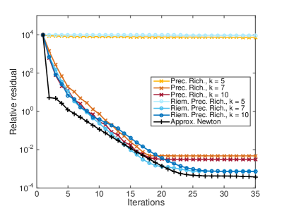
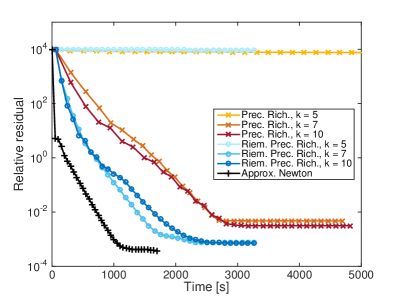
Figure 2: Newton potential with $d=3$. Comparison of truncated preconditioned Richardson, truncated Riemannian preconditioned Richardson, and the approximate Newton scheme when applied to the Newton potential in the Tucker format. For the Richardson iterations, exponential sum approximations with $k\in\{5,7,10\}$ terms are compared. Left: Relative residual as a function of iterations. Right: Relative residual as a function of time

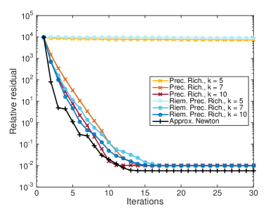
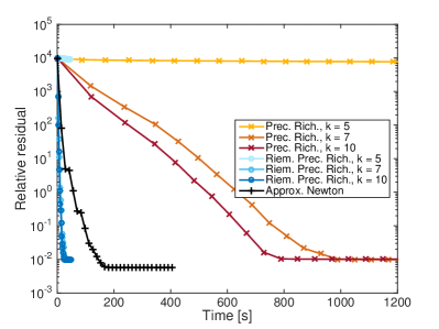
Figure 3: Anisotropic diffusion with $d=3$. Comparison of truncated Preconditioned Richardson, truncated Riemannian preconditioned Richardson, and the approximate Newton scheme when applied to the Newton potential in the Tucker format. For the Richardson iterations, exponential sum approximations with $k\in\{5,7,10\}$ terms are compared. Left: Relative residual as a function of iterations. Right: Relative residual as a function of time

With an accurate preconditioner, the truncated Richardson scheme converges fast with regard to the number of iterations, but suffers from very long computation times due to the exceedingly high intermediate ranks. In comparison, the Riemannian Richardson scheme yields similar convergence speed, but with significantly reduced computation time due to the additional projection into the tangent space. The biggest saving in computational effort comes from relation (26) which allows us to avoid having to form the preconditioned residual $\mathcal{P}^{-1}(\mathbf{F}-\mathcal{A}\mathbf{X}_{k})$ explicitly, a quantity with very high rank. Note that for both Richardson approaches, it is necessary to round the Euclidean gradient to lower rank using a tolerance of, say, $10^{-5}$ before applying the preconditioner to avoid excessive intermediate ranks.

The approximate Newton scheme converges equally well as the best Richardson approaches with regard to the number of iterations and does not require setting up a preconditioner. For the first test case, it only needs about half of the time as the best Richardson approach. For the second test case, it is significantly slower than Riemannian preconditioned Richardson. Since this operator is of lower rank than the Newton potential, the additional complexity of constructing the approximate Hessian does not pay off in this case.

Quadratic convergence.

In Figure 4 we investigate the convergence of the approximate Newton scheme when applied to a pure Laplace operator, $A=L$, and to the anisotropic diffusion operator $A=L+V$. In order to have an exact solution of known rank $r=4$, we construct the right hand side by applying $A$ to a random rank $4$ tensor. For the dimension and tensor size we have chosen $d=3$ and $n=200$, respectively. By construction, the exact solution lies on the manifold. Hence, if the approximate Newton method converges to this solution, we have zero residual and our Gauss–Newton approximation of (28) is an exact second-order model despite only containing the $A$ term. In other words, we expect quadratic convergence when $A=L$ but only linear when $A=L+V$ since our approximate Newton method (29) only solves with $L$. This is indeed confirmed in Figure 4.

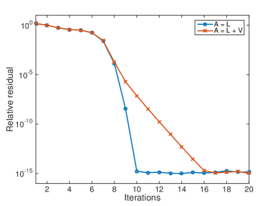
Figure 4: Convergence of the approximate Newton method for the zero-residual case when applied to a pure Laplace operator $L$ and to the anisotropic diffusion operator $L+V$.

5.4 Results for the TT format

In the TT format, we compare the convergence of our approximate Newton scheme (with the overlapping block-Jacobi preconditioner described in §4.3.2) to a standard approach, the alternating linear scheme (ALS).

We have chosen $d=60$, $n=100$, and a random rank-one right hand sides of norm one. In the first test case, the Newton potential, we have chosen TT ranks $r=10$ for the approximate solution. The corresponding convergence curves are shown in Figure 5. We observe that the approximate Newton scheme needs significantly less time to converge than the ALS scheme. As a reference, we have also included a steepest descent method using the overlapping block-Jacobi scheme directly as a preconditioner for every gradient step instead of using it to solve the approximate Newton equation (36). The additional effort of solving the Newton equation approximately clearly pays off.

In Figure 6, we show results for the anisotropic diffusion case. To obtain a good accuracy of the solution, we have to choose a relatively high rank of $r=25$ in this case. Here, the approximate Newton scheme is still faster, especially at the beginning of the iteration, but the final time needed to reach a residual of $10^{-4}$ is similar to ALS.

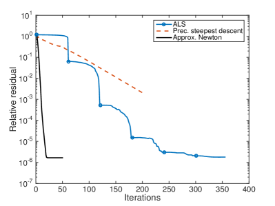
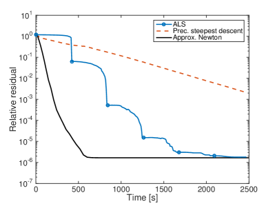
Figure 5: Newton potential with $d=60$. Convergence of ALS compared to preconditioned steepest descent with overlapping block-Jacobi as preconditioner and the approximate Newton scheme. Left: Relative residual as function of iterations. Right: Relative residual as function of time.

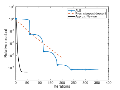
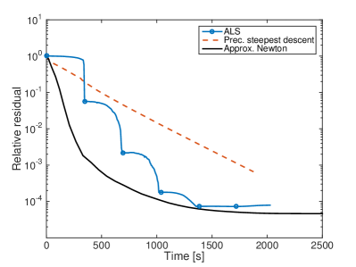
Figure 6: Anisotropic diffusion with $d=60$. Convergence of ALS compared to preconditioned steepest descent with overlapping block-Jacobi as preconditioner and the approximate Newton scheme. Left: Relative residual as function of iterations. Right: Relative residual as function of time.

Note that in Figures 5 and 6 the plots with regard to the number of iterations are to be read with care due to the different natures of the algorithms. One ALS iteration corresponds to the optimization of one core. In the plots, the beginning of each half-sweep of ALS is denoted by a circle. To assessment the performance of both schemes as fairly as possible, we have taken considerable care to provide the same level of optimization to the implementations of both the ALS and the approximate Newton scheme.

Mesh-dependence of the preconditioner.

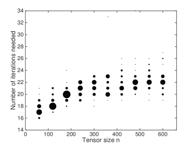
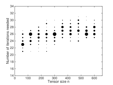
Figure 7: Number of iterations that the proposed approximate Newton scheme needs to reach a relative residual of $10^{-6}$ for different mesh widths $h=1/n$. The solution has dimension $d=10$ and rank $r=3$. We perform 30 runs for each size. The radii of the circles corresponds to the number of runs achieving this number of iterations. Left: Dimension $d=10$. Right: Dimension $d=30$.

To investigate how the performance of the preconditioner depends on the mesh width of the discretization, we look again at the anisotropic diffusion operator and measure the convergence as the mesh width $h$ and therefore the tensor size $n\in\{60,120,180,240,360,420,480,540,600\}$ changes by one order of magnitude. As in the test for quadratic convergence, we construct the right hand side by applying $A$ to a random rank $3$ tensor. For the dimension and tensor size we have chosen $d=3$ and $n=200$, respectively.

To measure the convergence, we take the number of iterations needed to converge to a relative residual of $10^{-6}$. For each tensor size, we perform 30 runs with random starting guesses of rank $r=3$. The result is shown in Figure 7, where circles are drawn for each combination of size $n$ and number of iterations needed. The radius of each circle denotes how many runs have achieved a residual of $10^{-6}$ for this number of iterations.

On the left plot of 7 we see the results of dimension $d=10$, whereas on the right plot we have $d=30$. We see that the number of iterations needed to converge changes only mildly as the mesh width varies over one order of magnitude. In addition, the dependence on $d$ is also not very large.

5.5 Rank-adaptivity

Note that in many applications, rank-adaptivity of the algorithm is a desired property. For the Richardson approach, this would result in replacing the fixed-rank truncation with a tolerance-based rounding procedure. In the alternating optimization, this would lead to the DMRG or AMEn algorithms. In the framework of Riemannian optimization, rank-adaptivity can be introduced by successive runs of increasing rank, using the previous solution as a warm start for the next rank. For a recent discussion of this approach, see [60]. A basic example of introducing rank-adaptivity to the approximate Newton scheme is shown in Figure 8. Starting from ranks $r^{(0)}=1$, we run the approximate Newton scheme for 10 iterations and use this result to warm start the algorithm with ranks $r^{(i)}=r^{(i-1)}+5$. At each rank, we perform 10 iterations of the approximate Newton scheme. The result is compared to the convergence of approximate Newton when starting directly with the target rank $r^{(i)}$. We see that the obtained relative residuals match for each of the ranks $r^{(i)}$. Although the adaptive rank scheme is slower for a desired target rank due to the additional intermediate steps, it offers more flexibility when we want to instead prescribe a desired accuracy. For a relative residual of $10^{-3}$, the adaptive scheme needs about half the time than using the (too large) rank $r=36$.

Note that in the case of tensor completion, rank adaptivity becomes a crucial ingredient to avoid overfitting and to steer the algorithm into the right direction, see e.g. [61, 33, 56, 60, 55]. For difficult completion problems, careful core-by-core rank increases become necessary. Here, for linear systems, such a core-by-core strategy does not seem to be necessary, as the algorithms will converge even if we directly optimize using rank $r=36$. This is likely due to the preconditioner which acts globally over all cores.

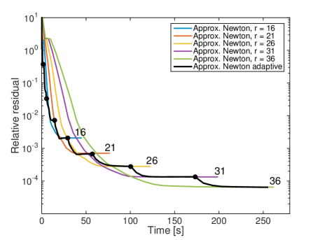
Figure 8: Rank-adaptivity for approximate Newton applied to the anisotropic diffusion equation with $n=100$, $d=10$. Starting from rank 1, the rank is increased by 5 after 10 iterations per rank. Each rank increase is denoted by a black circle. The other curves show the convergence when running approximate Newton directly with the target rank.

6 Conclusions

We have investigated different ways of introducing preconditioning into Riemannian gradient descent. As a simple but effective approach, we have seen the Riemannian truncated preconditioned Richardson scheme. Another approach used second-order information by means of approximating the Riemannian Hessian. In the Tucker case, the resulting approximate Newton equation could be solved efficiently in closed form, whereas in the TT case, we have shown that this equation can be solved iteratively in a very efficient way using PCG with an overlapping block-Jacobi preconditioner. The numerical experiments show favorable performance of the proposed algorithms when compared to standard non-Riemannian approaches, such as truncated preconditioned Richardson and ALS. The advantages of the approximate Newton scheme become especially pronounced in cases when the linear operator is expensive to apply, e.g., the Newton potential.

References

• [1] P.-A. Absil, R. Mahony, and R. Sepulchre. Optimization algorithms on matrix manifolds. Princeton University Press, Princeton, NJ, 2008.
• [2] P.-A. Absil, R. Mahony, and J. Trumpf. An extrinsic look at the Riemannian Hessian. In F. Nielsen and F. Barbaresco, editors, Geometric Science of Information, volume 8085 of Lecture Notes in Computer Science, pages 361–368. Springer Berlin Heidelberg, 2013.
• [3] P.-A. Absil and J. Malick. Projection-like retractions on matrix manifolds. SIAM J. Control Optim., 22(1):135–158, 2012.
• [4] I. Affleck, T. Kennedy, E. H. Lieb, and H. Tasaki. Rigorous results on valence-bond ground states in antiferromagnets. Phys. Rev. Lett., 59(7):799—802, 1987.
• [5] M. Bachmayr and W. Dahmen. Adaptive near-optimal rank tensor approximation for high-dimensional operator equations. Found. Comput. Math., 2014. To appear.
• [6] J. Ballani and L. Grasedyck. A projection method to solve linear systems in tensor format. Numer. Linear Algebra Appl., 20(1):27–43, 2013.
• [7] M. Benzi, G. H. Golub, and J. Liesen. Numerical solution of saddle point problems. Acta Numer., 14:1–137, 2005.
• [8] H. G. Bock. Randwertproblemmethoden zur Parameteridentifizierung in Systemen nichtlinearer Differentialgleichungen. Bonner Math. Schriften, 1987.
• [9] N. Boumal and P.-A. Absil. RTRMC: A Riemannian trust-region method for low-rank matrix completion. In Proceedings of the Neural Information Processing Systems Conference (NIPS), 2011.
• [10] D. Braess and W. Hackbusch. Approximation of $1/x$ by exponential sums in $[1,\infty)$. IMA J. Numer. Anal., 25(4):685–697, 2005.
• [11] C. Da Silva and F. J. Herrmann. Hierarchical Tucker tensor optimization – applications to tensor completion. Linear Algebra Appl., 2015. To appear.
• [12] L. De Lathauwer, B. De Moor, and J. Vandewalle. A multilinear singular value decomposition. SIAM J. Matrix Anal. Appl., 21(4):1253–1278, 2000.
• [13] S. V. Dolgov. TT-GMRES: solution to a linear system in the structured tensor format. Russian J. Numer. Anal. Math. Modelling, 28(2):149–172, 2013.
• [14] S. V. Dolgov and I. V. Oseledets. Solution of linear systems and matrix inversion in the TT-format. SIAM J. Sci. Comput., 34(5):A2718–A2739, 2012.
• [15] S. V. Dolgov and D. V. Savostyanov. Alternating minimal energy methods for linear systems in higher dimensions. SIAM J. Sci. Comput., 36(5):A2248–A2271, 2014.
• [16] L. Grasedyck. Existence and computation of low Kronecker-rank approximations for large linear systems of tensor product structure. Computing, 72(3–4):247–265, 2004.
• [17] L. Grasedyck. Hierarchical singular value decomposition of tensors. SIAM J. Matrix Anal. Appl., 31(4):2029–2054, 2010.
• [18] L. Grasedyck, D. Kressner, and C. Tobler. A literature survey of low-rank tensor approximation techniques. GAMM-Mitt., 36(1):53–78, 2013.
• [19] W. Hackbusch. Entwicklungen nach Exponentialsummen. Technical Report 4/2005, MPI MIS Leipzig, 2010. Revised version September 2010.
• [20] W. Hackbusch. Tensor Spaces and Numerical Tensor Calculus. Springer, Heidelberg, 2012.
• [21] W. Hackbusch and B. N. Khoromskij. Low-rank Kronecker-product approximation to multi-dimensional nonlocal operators. I. Separable approximation of multi-variate functions. Computing, 76(3-4):177–202, 2006.
• [22] W. Hackbusch and S. Kühn. A new scheme for the tensor representation. J. Fourier Anal. Appl., 15(5):706–722, 2009.
• [23] J. Haegeman, M. Mariën, T. J. Osborne, and F. Verstraete. Geometry of matrix product states: Metric, parallel transport and curvature. J. Math. Phys., 55(2), 2014.
• [24] S. Holtz, T. Rohwedder, and R. Schneider. The alternating linear scheme for tensor optimization in the tensor train format. SIAM J. Sci. Comput., 34(2):A683–A713, 2012.
• [25] S. Holtz, T. Rohwedder, and R. Schneider. On manifolds of tensors of fixed TT-rank. Numer. Math., 120(4):701–731, 2012.
• [26] V. Kazeev, O. Reichmann, and Ch. Schwab. Low-rank tensor structure of linear diffusion operators in the TT and QTT formats. Lin. Alg. Appl., 438(11):4204–4221, 2013.
• [27] B. N. Khoromskij and I. V. Oseledets. Quantics-TT collocation approximation of parameter-dependent and stochastic elliptic PDEs. Comput. Meth. Appl. Math., 10(4):376–394, 2010.
• [28] B. N. Khoromskij, I. V. Oseledets, and R. Schneider. Efficient time-stepping scheme for dynamics on TT-manifolds. Technical Report 24, MPI MIS Leipzig, 2012.
• [29] B. N. Khoromskij and Ch. Schwab. Tensor-structured Galerkin approximation of parametric and stochastic elliptic PDEs. SIAM J. Sci. Comput., 33(1):364–385, 2011.
• [30] O. Koch and Ch. Lubich. Dynamical tensor approximation. SIAM J. Matrix Anal. Appl., 31(5):2360–2375, 2010.
• [31] T. G. Kolda and B. W. Bader. Tensor decompositions and applications. SIAM Review, 51(3):455–500, 2009.
• [32] D. Kressner, M. Plešinger, and C. Tobler. A preconditioned low-rank CG method for parameter-dependent Lyapunov matrix equations. Numer. Linear Algebra Appl., 21(5):666–684, 2014.
• [33] D. Kressner, M. Steinlechner, and A. Uschmajew. Low-rank tensor methods with subspace correction for symmetric eigenvalue problems. SIAM J. Sci. Comput., 36(5):A2346–A2368, 2014.
• [34] D. Kressner, M. Steinlechner, and B. Vandereycken. Low-rank tensor completion by Riemannian optimization. BIT, 54(2):447–468, 2014.
• [35] D. Kressner and C. Tobler. Krylov subspace methods for linear systems with tensor product structure. SIAM J. Matrix Anal. Appl., 31(4):1688–1714, 2010.
• [36] D. Kressner and C. Tobler. Low-rank tensor Krylov subspace methods for parametrized linear systems. SIAM J. Matrix Anal. Appl., 32(4):1288–1316, 2011.
• [37] D. Kressner and C. Tobler. Preconditioned low-rank methods for high-dimensional elliptic PDE eigenvalue problems. Comput. Methods Appl. Math., 11(3):363–381, 2011.
• [38] D. Kressner and C. Tobler. Algorithm 941: htucker – a Matlab toolbox for tensors in hierarchical Tucker format. TOMS, 40(3), 2014.
• [39] C. Lubich, I. Oseledets, and B. Vandereycken. Time integration of tensor trains. arXiv preprint 1407.2042, 2014.
• [40] C. Lubich, I. V. Oseledets, and B. Vandereycken. Time integration of tensor trains. SIAM J. Numer. Anal., 53(2):917–941, 2015.
• [41] Ch. Lubich. From quantum to classical molecular dynamics: reduced models and numerical analysis. Zurich Lectures in Advanced Mathematics. European Mathematical Society (EMS), Zürich, 2008.
• [42] D. G. Luenberger. The gradient projection method along geodesics. Management Science, 18(1):620–631, 1970.
• [43] B. Mishra, G. Meyer, S. Bonnabel, and R. Sepulchre. Fixed-rank matrix factorizations and Riemannian low-rank optimization. Comput. Statist., 29(3-4):591–621, 2014.
• [44] B. Mishra and R. Sepulchre. R3MC: A Riemannian three-factor algorithm for low-rank matrix completion. In Decision and Control (CDC), 53rd Annual Conference on, pages 1137–1142. IEEE, 2014.
• [45] B. Mishra and R. Sepulchre. Riemannian preconditioning. arXiv preprint 1405.6055, 2014.
• [46] Y. Nesterov. Introductory lectures on convex optimization, volume 87 of Applied Optimization. Kluwer Academic Publishers, Boston, MA, 2004. A basic course.
• [47] T. Ngo and Y. Saad. Scaled gradients on Grassmann manifolds for matrix completion. In F. Pereira, C. J. C. Burges, L. Bottou, and K. Q. Weinberger, editors, Advances in Neural Information Processing Systems 25, pages 1412–1420. Curran Associates, Inc., 2012.
• [48] J. Nocedal and S. J. Wright. Numerical Optimization. Springer Series in Operations Research. Springer, 2nd edition, 2006.
• [49] I. V. Oseledets. DMRG approach to fast linear algebra in the TT–format. Comput. Meth. Appl. Math, 11(3):382–393, 2011.
• [50] I. V. Oseledets. Tensor-train decomposition. SIAM J. Sci. Comput., 33(5):2295–2317, 2011.
• [51] H. Rauhut, R. Schneider, and Z. Stojanac. Tensor completion in hierarchical tensor representations. In H. Boche, R. Calderbank, G. Kutyniok, and J. Vybíral, editors, Compressed Sensing and its Applications: MATHEON Workshop 2013, Applied and Numerical Harmonic Analysis, pages 419–450. Birkhäuser Basel, 2015.
• [52] T. Rohwedder and A. Uschmajew. On local convergence of alternating schemes for optimization of convex problems in the tensor train format. SIAM J. Numer. Anal., 51(2):1134–1162, 2013.
• [53] U. Schollwöck. The density-matrix renormalization group in the age of matrix product states. Ann. Physics, 326:96–192, 2011.
• [54] V. Simoncini. Computational methods for linear matrix equations, 2013. Preprint available from http://www.dm.unibo.it/~simoncin/list.html.
• [55] M. Steinlechner. Riemannian Optimization for High-Dimensional Tensor Completion. Technical report MATHICSE 5.2015, EPF Lausanne, Switzerland, 2015.
• [56] M. Tan, I. Tsang, L. Wang, B. Vandereycken, and S. Pan. Riemannian pursuit for big matrix recovery. In ICML 2014, volume 32, pages 1539–1547, 2014.
• [57] L. Tucker. Some mathematical notes on three-mode factor analysis. Psychometrika, 31:279–311, 1966.
• [58] A. Uschmajew. Zur Theorie der Niedrigrangapproximation in Tensorprodukten von Hilberträumen. PhD thesis, Technische Universität Berlin, 2013.
• [59] A. Uschmajew and B. Vandereycken. The geometry of algorithms using hierarchical tensors. Linear Algebra Appl., 439(1):133–166, 2013.
• [60] A. Uschmajew and B. Vandereycken. Greedy rank updates combined with Riemannian descent methods for low-rank optimization. In Sampling Theory and Applications (SampTA), 2015 International Conference on, pages 420–424. IEEE, 2015.
• [61] B. Vandereycken. Low-rank matrix completion by Riemannian optimization. SIAM J. Optim., 23(2):1214—1236, 2013.
• [62] B. Vandereycken and S. Vandewalle. A Riemannian optimization approach for computing low-rank solutions of Lyapunov equations. SIAM J. Matrix Anal. Appl., 31(5):2553–2579, 2010.
• [63] J. Xu. Iterative methods by space decomposition and subspace correction. SIAM Rev., 34(4):581–613, 1992.
• [64] J. Xu. The method of subspace corrections. J. Comput. Appl. Math., 128(1-2):335–362, 2001. Numerical analysis 2000, Vol. VII, Partial differential equations.