From Cutting Planes Algorithms to Compression Schemes and Active Learning

Abstract

Cutting-plane methods are well-studied localization (and optimization) algorithms. We show that they provide a natural framework to perform machine learning —and not just to solve optimization problems posed by machine learning— in addition to their intended optimization use. In particular, they allow one to learn sparse classifiers and provide good compression schemes. Moreover, we show that very little effort is required to turn them into effective active learning methods. This last property provides a generic way to design a whole family of active learning algorithms from existing passive methods. We present numerical simulations testifying of the relevance of cutting-plane methods for passive and active learning tasks.

I Introduction

We show that localization methods based on cutting planes provide a natural framework to derive machine learning algorithms for classification, both in the supervised learning framework and the active learning framework. Our claim is that cutting plane algorithms, beyond their optimization purposes, embed features that are beneficial for generalization purposes. In particular a) under mild conditions, they may provide compression scheme with a compression rate that is directly related to their aim at rapidly finding a solution of the localization problem and b) the pivotal step of such algorithms, namely, the querying step, may be slightly twisted so as to be active-learning friendly.

In the present paper, we show that existing learning algorithms might be revisited from the cutting planes point of view. Not only might the active learning SVM procedure of Tong and Koller [1] be reinterpreted as an algorithm falling under the framework we describe but so are the Bayes Point Machines [2], for which we will propose an active learning version of it.

The problems we are interested in are linear classification problems. Given a training sample $D\doteq\{(x_{n},y_{n})\}_{n\in[N]}$, with $x_{n}\in{\cal X}\doteq\mathbb{R}^{d},$ $y_{n}\in{\cal Y}\doteq\{-1,+1\},$ and $[N]\doteq\{1,\ldots,N\}$, we are looking for a classification vector $w\in{\cal X}$ that is an element of the version space

$${\cal W}_{0}(D)\doteq\left\{w\in{\cal X}:y_{n}\langle w,x_{n}\rangle\geq 0,\;n\in[N]\right\},$$ (1)

of $D$, i.e. the set of vectors $w$ from ${\cal X}$ such that the corresponding linear predictors

$$f_{w}(x)\doteq\text{sign}(\langle w,x\rangle)$$ (2)

make no mistake on the training set $D.$ In order to render the exposition clearer, we make the assumption that the training data are linearly separable so that ${\cal W}_{0}(D)$ is not empty. The case where ${\cal W}_{0}(D)=\emptyset$ can be tackled with usual machine learning techniques —e.g. the “$\lambda$-trick” and/or kernels [3] [2].

Also, for the sake of brevity, we may use ${\cal W}_{0}$ instead of ${\cal W}_{0}(D)$ and thus drop the explicit dependence on $D.$

With the relevant notation at hand, the problem we are interested in may be stated as:

$$\operatorname*{\text{find }}w\in{\cal W}_{0},$$ (3)

which might be simply rewritten as the problem of solving a set of linear inequalities

$$\operatorname*{\text{find }}w\enskip\text{ s.t. } \left\{\begin{array}[]{l}w\in{\cal X}\\ y_{n}\left\langle w,x_{n}\right\rangle\geq 0,\;n\in[N].\end{array}\right.$$ (6)

There is a variety of methods in the optimization literature from as back as the 50’s that are available to solve such problems. Among them, we may mention (over-)relaxation based methods [4, 5], simplex-based algorithms and, of course, the Perceptron algorithm and its numerous variants [6, 7, 8]. Localization methods based on cutting planes, or, in short, cutting planes algorithms, are well-studied algorithms, well-known to be very efficient to solve such problems. We will show that, when used to solve (6), i) they naturally provide compression scheme algorithms [9], and thus, learning algorithms that embed features designed to ensure good generalization properties and ii) they also set the ground for the development of new active learning algorithms.

I-A Related Works

Cutting-plane methods provide a family of optimizaton procedures that have received some interest from the machine learning community [10, 11, 12]. However, they have mainly been considered as optimization methods to solve problems such as those posed by support vector machines or, more generally, regularized risk functionals. The more profound connection of these methods with learning algorithms, that is, procedures that are designed in a way to ensure generalization ability to the predictor they build (e.g. the Perceptron algorithm) has less been studied; this is one of the peculiarities of the present paper to discuss this feature—to some extent, the work of [12], which pinpoints how statistical regularization is beneficial for the stabilization of cutting-plane methods, skims over this connection. Within the vast literature of active learning (see, e.g. [13]), we may single out a few contributions our work is closely related to; they share the common feature of focusing on/exploiting the geometry of the version space. The query strategies proposed by [14] and [15] are based on multiple estimations of the volume of the (potential) version space, which, when added together might be computationally expensive. In comparison, in the active learning strategy we derive from the general cutting-plane approach, we compute our queries from an approximated center of gravity of the version space, which is computationally equivalent to a single volume estimation. The work of [16], who propose a margin-based query strategy provide theoretical justifications of such strategies and gives insights on the foundations the work of [1] hinges on. Our contribution is to show how the cutting planes literature and its accompanying worst-case convergence analyzes may give rise to theoretically supported query strategies that do not have to hinge on margin-based arguments. To some extent, our work has connections with uncertainty-based active learning (see, e.g. [17]) which advocates to query the points whose class is the most uncertain; our approach may be re-interpreted as a theoretically motivated uncertainty measure based on the volume reduction of the version space.

I-B Outline

The paper is structured as follows. Section II provides some background to cutting planes methods and their possible application to learning. Section III further explores the connections between cutting planes and learning algorithms and then provides a way to turn cutting planes methods into an active learning algorithms. Section IV reports empirical results for algorithms derived from our argumentation on the relevance of cutting plane methods to machine learning.

II Background

In this section, we first recall the general form of a cutting plane algorithm to solve a localization problem. We then specialize this algorithm to the case where the convex space into which we want to find a point is the version space associated to training set $D$. Finally, in order for the reader to get a taste on how cutting planes algorithms give rise to learning algorithms, i.e. algorithms that embed features, namely, they define compression schemes with targeted small compression size, that are beneficial for generalization.

II-A Vanilla Localization Algorithm with Cutting Planes

In order to solve a problem like

$$\operatorname*{\text{find }}w\in{\cal C},$$

for ${\cal C}$ some closed convex set, a localization algorithm based on cutting planes works as follows (see also the synthetic depiction in Algorithm 1) [18]. The algorithm maintains and iteratively refines (i.e. reduces) a closed convex set ${\cal C}^{t}$ that is known to contain ${\cal C}$. From ${\cal C}^{t}$ a query point is computed —there are several ways to compute such query points; we will mention some when specializing localization methods to the specific problem of finding a point in the version space later on— which leads to two possible options: either a) $w^{t}$ is in ${\cal C}$ and the tackled problem is solved or b) $w^{t}\not\in{\cal C}$. In the latter case, a so-called cutting plane oracle is queried with $w^{t}$ upon which it returns the parameters $(a_{t},b_{t})$ of the hyperplane $\{z:\langle a_{t},z\rangle=b_{t}\}$ such that this hyperplane separates $w_{t}$ from ${\cal C}$, i.e., $\forall w\in{\cal C},\langle a_{t},w\rangle>b_{t}$ and $\langle a_{t},w_{t}\rangle\leq b_{t}$. The hyperplane is used to reduce ${\cal C}^{t}$ into ${\cal C}^{t}\cap\{w:\langle a_{t},w\rangle>b_{t}\}$ (which still contains ${\cal C}$). For the specific problem (6) of finding a point in the version space, the cutting planes rendered by the oracle will be such that $b_{t}=0$.

Algorithm 1 Classical Cutting Plane Algorithm for the localization of $w\in{\cal C}$.

1:$w\in{\cal C}$

2:compute ${\cal C}^{0}$, such that ${\cal C}^{0}\supset{\cal C}$ and ${\cal C}^{0}$ is convex and closed.

3:$t\leftarrow 0$

4:repeat

5:     Compute query point $w^{t}$ in ${\cal C}^{t}$

6:     Ask the cutting plane oracle whether $w^{t}\in{\cal C}$

7:     if  $w^{t}\notin{\cal C}$  then

8:         Receive a cutting plane $(a_{t},b_{t})$

9:         ${\cal C}^{t+1}\leftarrow{\cal C}^{t}\cap\left\{x:\langle a_{t},x\rangle>b_{t}\right\}$

10:         $t\leftarrow t+1$

11:     end if

12:until $w^{t}\in{\cal C}$

13:return $w^{t}$

Algorithm 2 The Cutting Plane approach instantiated to the problem of finding a point from the version space of $D$.

1:$w$ solution of Problem (11)

2:${\cal C}^{0}\leftarrow{\cal B}$

3:$t\leftarrow 0$

4:repeat

5:     $w^{t}\leftarrow\textsc{Query}({\cal C}^{t})$ $\triangleright$ Compute query point $w^{t}$ in ${\cal C}^{t}$

6:     if $w^{t}\notin{\cal W}$ then

7:         $n_{t}\leftarrow\textsc{Pick}({\cal C}^{t},w^{t})$ $\triangleright$ pick a cutting plane index

8:         ${\cal C}^{t+1}\leftarrow{\cal C}^{t}\cap\left\{z:y_{n_{t}}\langle z,x_{n_{t}}\rangle>0\right\}$

9:         $t\leftarrow t+1$

10:     end if

11:until $w^{t}\in{\cal W}$

12:return $w^{t}$

II-B Cutting Planes to Localize a Point in the Version Space

Note that problem (6) is scale-insensitive: if $w\in{\cal W}_{0}$, then $\lambda w\in{\cal W}_{0}$ as well for any $\lambda>0.$ In order to get rid of this degree of freedom and to make the use of cutting planes algorithms possible (they require the sets ${\cal C}^{t}$ to be bounded), we will restrict ourselves to finding a solution vector $w^{*}$ both in ${\cal W}_{0}$ and in the unit ball

$${\cal B}\doteq\left\{w\in{\cal X}:\|w\|\leq 1\right\}.$$ (7)

In other words, we will be looking for $w^{*}$ in the constrained version space

$${\cal W}\doteq{\cal W}_{0}\cap{\cal B},$$ (8)

and the problem we face is therefore:

$$\operatorname*{\text{find }}w\enskip\text{ such that } \left\{\begin{array}[]{l}w\in{\cal B}\\ y_{n}\langle w,x_{n}\rangle\geq 0,\;n\in[N]\end{array}\right.$$ (11)

In the case of Problem (11), the localization algorithm described earlier translates into the one given in Algorithm 2. The following changes might be observed when comparing with Algorithm 1: ${\cal C}^{0}$ is now initialized to ${\cal B}$, the unit ball, and the cutting planes are picked among the hyperplanes —i.e. the points of $D$— defining the version space.

II-C Query Point Generation

In both Algorithm 1 and Algorithm 2, the strategy to compute a query point is left unspecified. There actually exist many ways to compute such query points, but they all aim at a query point which calls for a cutting plane that will divide the current enclosing convex set ${\cal C}^{t}$ in the most stringent way. It turns out that such guarantee might be expected when the query point is as close as possible to the ‘center’ of ${\cal C}^{t}$, so that the volume of ${\cal C}^{t}$ is reduced with a positive factor —just as in the well-known bisection method, where the factor is 1/2. The center of ${\cal C}^{t}$ is not defined in a unique way, but for the most popular query methods, it may refer to: a) the center of gravity of ${\cal C}^{t}$, b) the center of the largest ball inscribed in ${\cal C}^{t}$, which is called the Chebyshev center or c) the analytic center, which we will not discuss further (the interested reader may refer to [19] for further details). We may mention three things regarding the center of gravity: i) it is NP-hard to exactly compute the center of gravity of a convex set in an arbitrary $n$-dimensional space even though some practical approximation algorithms exist; ii) it is the query point that comes with the best guarantees in terms of convergence speed of the cutting plane method [20]; iii) the center of gravity of a polytope is precisely the point that is looked for in the case of the theoretically founded Bayes Point Machines of [2].

III Results

This section is devoted to some algorithmic results that can be obtained when analyzing the behavior of cutting-plane methods for the localization of a point in the version space.

III-A Cutting Planes Provide Sample Compression Schemes

Let ${\cal D}\doteq\bigcup_{n=1}^{\infty}({\cal X}\times{\cal Y})^{n}$ be the set of all finite training samples made of pairs from ${\cal X}\times{\cal Y}$. In short, sample compression schemes [9] are learning algorithms ${\cal A}:{\cal D}\rightarrow{\cal Y}^{{\cal X}}$ that are associated with a compression function ${\cal S}:{\cal D}\rightarrow{\cal D}$ so that, given any training sample $D$, we have ${\cal A}(D)={\cal A}({\cal S}(D)).$ Sample compression schemes are especially interesting when the size $|{\cal S}(D)|$ of the compression set ${\cal S}(D)$ is small. Indeed, generalization guarantees that come with these procedures say that the generalization error of $f_{D}\doteq{\cal A}(D)$ is, with high probability (over the random draw of training set $D$ according to an unknown and fix distribution) bounded from above by something like

$$\frac{1}{N-|{\cal S}(D)|}\sum_{n=1}^{N}\mathbb{I}\left[f_{D}(x_{n})\neq y_{n}\right]+\mathcal{O}\left(\sqrt{\frac{1}{N-|{\cal S}(D)|}}\right)$$ (12)

(see [9, 21] for a precise statement of the bound). Among the most well-known learning compression schemes, we find the Perceptron and the Support Vector Machines.

We claim that Algorithm 2, which finds a point in the version space using cutting planes, may be a compression scheme.

Proposition 1.

If $\textsc{Query}({\cal C}^{t})$ (line 5, Algorithm 2) and $\textsc{Pick}({\cal C}^{t},w^{t})$ (line 7) are both deterministic then Algorithm 2 is a sample compression scheme.

Proof.

If the compression set is made of the training examples that define the cutting planes, this result is a direct consequence of the structure of Algorithm 2. A proof by induction that essentially hinges on the fact that, at each iteration $t$, the next query point is deterministically computed from ${\cal C}^{t}$ (only) gives the result. ∎

A few observations can be made. First, the learning algorithm obtained with the assumptions of Proposition 1 is a process sample compression scheme, that is, even if we interrupt the learning before convergence has occurred, running the algorithm on the partial compression scheme obtained so far gives exactly the same predictor. Second, it is obviously an aim to have fast convergence of the localization procedure, where fast convergence means few iterations of the cutting-plane procedure. This directly translates into the idea of finding a point in the version space that is expressed as a combination as few vectors as possible, which, by (12), is very beneficial for generalization purposes. Later, we will see that there are settings for cutting-plane methods that come with guarantees on the number of iterations, and therefore on $|{\cal S}(D)|$, to reach convergence.

1:Problem (11)

2:${\cal C}^{0}\leftarrow{\cal B}$

3:$t\leftarrow 1$, $w^{0}\leftarrow 0$, $\tilde{w}^{0}\leftarrow 0$

4:repeat

5:     $\tilde{w}^{t}\leftarrow\textsc{Perceptron}(\tilde{w}^{t-1},x_{n_{0}},\cdots,x_{n_{t}})$

6:     $w^{t}\leftarrow{\tilde{w}^{t}}/{\|\tilde{w}^{t}\|_{2}}$

7:     if $w^{t}\notin{\cal W}$ then

8:         Pick a cutting plane index $n_{t}$

9:         ${\cal C}^{t+1}\leftarrow{\cal C}^{t}\cap\left\{z:y_{n_{t}}\langle z,x_{n_{t}}\rangle\geq 0\right\}$

10:         $t\leftarrow t+1$

11:     end if

12:until $w^{t}\in{\cal W}$

13:return $w^{t}$

14:

15:function Perceptron($w^{start},x_{n_{0}},\cdots,x_{n_{N}}$)

16:     $t\leftarrow 0$

17:     $w^{0}\leftarrow w^{start}$

18:     while $\exists n_{i}:\langle w^{t},x_{n_{i}}\rangle<0$ do

19:         $w^{t+1}\leftarrow w^{t}+x_{n_{i}}$

20:         $t\leftarrow t+1$

21:     end while

22:     return $w^{t}$

23:end function

Algorithm 3 Top : A Perceptron-based localization algorithm for the case of problem (11). Bottom : The slightly modified perceptron algorithm for compression scheme.

III-B Perceptron-based Localization Algorithm

One of the simplest ways to compute a query point $w^{t}$ for Algorithm 2 is to run Rosenblatt’s Perceptron algorithm [8] at each step and query the normalized solution $w^{t}={\tilde{w}^{t}}/{\|\tilde{w}^{t}\|_{2}}$. Intuitively, we may expect $\tilde{w}^{t+1}$ to be ‘close’ to $\tilde{w}^{t}$ because ${\cal C}^{t+1}$ is essentially the intersection of ${\cal C}^{t}$ with a cutting plane and much of the geometry of ${\cal C}^{t}$ might be preserved. According to this intuition, $\tilde{w}^{t}$ should be a good starting point for the Perceptron algorithm to be run and to have it output $\tilde{w}_{t+1}$. Algorithm 3 implements that idea, and reuses the last query point as an initialization vector for the Perceptron to compute the next query point. Additionally, note that for Algorithm 3 to match Proposition 1 a little technicality is needed: we require that datapoints are selected in the lexicographical order when multiple choices are possible (e.g. line 8 and 18). It turns out this simple querying procedure enjoys the same convergence rate than a regular Perceptron, with the added empirically observed benefit of providing stronger compression (see Section IV for empirical results).

Proposition 2.

Consider Problem (11) and let $\gamma$ be the radius of the largest inscribed sphere in ${\cal W}$. Define $M$ the number of Perceptron updates performed by the Perceptron-based Localization Algorithm 3 (i.e. $M$ is the number of times line 19 of Perceptron() of Algorithm 3 is executed). Then the following holds: $M\leq 1/{\gamma^{2}}$.

Proof.

We recall that the usual definition of the margin of $D$ is $\min_{x\in D}\langle w^{*},x\rangle$ and note that $\gamma$ is related to it since $\forall n\in[N],\;\langle w^{*},x_{n}\rangle/\|x_{n}\|_{2}\geq\gamma$. Let ${\cal S}\doteq\{a_{1},\ldots a_{M}\}$ be the sequence of points used to perform Perceptron updates across a complete execution of Algorithm 3. Thus, ${\cal S}$ is a sequence from $D$ (with possible duplicates) and $w^{*}$ achieves a margin at least $\gamma$ with all points in ${\cal S}$. From [6, 7] we know that the number $M$ of Perceptron updates on any arbitrary sequence linearly separable with margin $\gamma$ is no more than $1/{\gamma^{2}}$. Since we use $w^{t}$ as a starting point to compute $w^{t+1}$, the execution of the cutting-plane algorithm is tied to the execution of the Perceptron algorithm on ${\cal S}$. Therefore, there is less than $1/{\gamma^{2}}$ Perceptron updates during the execution of the algorithm. Alternatively, $|{\cal S}|\leq 1/{\gamma^{2}}$ since all points in ${\cal S}$ correspond to a Perceptron update, thus a mistake. ∎

On a side note, the same argument can be applied to obtain similar results with most Perceptron-like learning procedures (see for instance [22, 23]).

III-C Center of Gravity and Approximations

Figure 1: An Example of version space where the Chebyshev Center (light blue) is a bad approximation of the gravity center (dark blue).

The question of computing a query point $w^{t}$ is of central importance in cutting-plane localization algorithms. As we have seen, a simple Perceptron can already yield interesting computational results for that matter. A more assiduous analysis of this question can be conducted by looking at the volume reduction $\text{V}({\cal C}^{t+1})/\text{V}({\cal C}^{t})$ of ${\cal C}^{t}$ from one iteration to the next. The notion of center of gravity is going to be pivotal to this end.

Definition 1 (Center of Gravity).

Let ${\cal C}$ be a closed set in $\mathbb{R}^{n}$. The center of gravity (CG) $\textbf{cg}({\cal C})$ of ${\cal C}$ is defined by as $\textbf{cg}({\cal C})\doteq\int_{{\cal C}}zdz/\int_{{\cal C}}dz.$

The center of gravity is deeply tied to the volume of ${\cal C}^{t}$ and plays a central role in devising cutting-plane algorithms for which the volume reduction $\text{V}({\cal C}^{t+1})/\text{V}({\cal C}^{t})$ is the largest. Theorem 1 reports one of the most fundamental property of the center of gravity (see [24, 25, 26, 27])

Theorem 1 (Partition of Convex bodies).

Let ${\cal C}\in\mathbb{R}^{d}$ a convex body of center of gravity $\textbf{cg}({\cal C})$ and $h$ a hyperplane such that $\textbf{cg}({\cal C})\in h$. Thus, $h$ divide ${\cal C}$ in two subsets ${\cal C}_{1}$ and ${\cal C}_{2}$ and the following relations hold for $i=1,2$: $\text{V}({\cal C}_{i})\geq e^{-1}\text{V}({\cal C})$

The center of gravity method proposed by [25, 26] consists in querying $w^{t}=\textbf{cg}({\cal C}^{t})$ and typically have a very fast convergence rate as the version space is almost halved at each step. More precisely, a direct consequence of Theorem 1 is that the volume of ${\cal C}^{t}$ is bounded by $\text{V}({\cal C}^{t})\leq(1-1/e)^{t}\text{V}({\cal C}^{0})$. However, computing the center a gravity is hard, making the center of gravity method impractical. Instead, one has to consider structural or numerical approximations to the center of gravity.

Definition 2 (Chebyshev’s Center).

Let ${\cal C}$ a set in $\mathbb{R}^{n}$. Chebyshev’s center (CC) of ${\cal C}$, $\textbf{cc}({\cal C})$ is the center of the largest inscribed ball in ${\cal C}$:

$$\textbf{cc}({\cal C})=\arg\min_{\hat{z}}\max_{z}\|z-\hat{z}\|_{2}^{2}.$$

Chebyshev’s center is used as a computationally efficient approximation of the center of gravity for cutting-plane algorithms since the late 70’s [28] (see, e.g. [29] for a linear formulation of the problem). Unfortunately, the interesting property of Theorem 1 does not carry over with Chebyshev’s center. One problem in machine learning related to Chebyshev’s center is the extensively studied Support Vector Machine (Svm) [30] defined as :

$$\min_{w}\frac{1}{2}\|w\|_{2}^{2}\enskip\text{ s.t. } \left\{\begin{array}[]{l}w\in{\cal X}\\ y_{n}\left\langle w,x_{n}\right\rangle\geq 1,\;n\in[N].\end{array}\right.$$ (15)

A notable property of the Svm is that its solution $w_{\text{\sc Svm}}$ is closely related to the center of the largest inscribed ball in ${\cal W}$ and is an approximation of the center of gravity [2]. Indeed, $w_{\text{\sc Svm}}$ is actually a rescaled Chebyshev’s center [1] [2].

On the other hand, numerical approximations aim at finding a point that is in the close neighborhood of the center of gravity. One of the contributions of this paper is to give a generalized version of Theorem 1 for approximations of the center of gravity, thus laying a theoretical justification for these methods.

Theorem 2 (Generalized Partition of Convex bodies).

Let ${\cal C}$ be a closed convex body in $\mathbb{R}^{d}$ and $\textbf{cg}({\cal C})$ its center of gravity. Let $h_{x}$ a hyperplane of normal vector $x$, $\|x\|_{2}=1$ and define the upper (resp. lower) partition ${\cal C}^{+}$ (resp. ${\cal C}^{-}$) of ${\cal C}$ by $h_{x}$ as

$${\cal C}^{+}\doteq{\cal C}\cap\left\{w\in\mathbb{R}^{d}:\langle x,w\rangle\geq 0\right\}$$

$${\cal C}^{-}\doteq{\cal C}\cap\left\{w\in\mathbb{R}^{d}:\langle x,w\rangle<0\right\}.$$

The following holds true: if $\textbf{cg}({\cal C})+\Lambda x\in{\cal C}^{+}$ then

$$\text{V}({\cal C}^{+})/\text{V}({\cal C})\geq e^{-1}(1-\lambda)^{d},$$

where

$$\Lambda=\lambda\Theta_{d}\frac{\text{V}({\cal C})H_{{\cal C}^{+}}}{R^{d}H_{{\cal C}^{-}}},$$

with $\lambda\in\mathbb{R}$ an arbitrary real, $\Theta_{d}$ a constant depending only on $d$, $R$ the radius of the $(d-1)$-dimensional ball $B$ of volume $\text{V}\left[B\right]\doteq\text{V}\left[{\cal C}\cap\left\{w\in\mathbb{R}^{d}:\langle x,w\rangle=0\right\}\right]$ and $H_{{\cal C}^{+}}=\max_{a\in{\cal C}^{+}}a^{T}x$ (resp. $H_{{\cal C}^{-}}=\min_{a\in{\cal C}^{-}}a^{T}x$)

Proof.

The proof is a (non-trivial) extension of Grunbaum’s one for Theorem 1 [24]. Due to space restriction, we cannot expose it here in full and refer the interested reader to http://pageperso.lif.univ-mrs.fr/~ugo.louche/paper/activeCPSuppl.pdf ∎

Theorem 2 extends Theorem 1 to the situation when an approximation of the center of gravity is considered; it reduces to Theorem 1 when applied to the very center of gravity. This is to the best of our knowledge the first result of this kind and this is a result that is of its own interest, wich may benefit to many fields of computer science. Here, the purpose of Theorem 2 is essentially to validate the use of approximations of the center of gravity $\textbf{cg}({\cal C})$ in the procedures at hand, which is inevitable due to the complexity of exactly finding this point. We will more precisely use it in two occasions: a) for center-of-gravity-based compression scheme methods and b) in the active learning setting (see below).

III-D Active Learning with Cutting Planes

An interesting situation of learning is that of active learning when the algorithm is presented with unlabelled data and it has to query for the labels of the training points that carry the most information to build a relevant decision boundary. Given a volume ${\cal C}$ inside which a good classifier $w^{*}$ for the classification task at hand is known to lie, the amount of information carried by a labeled training point $(x,y)$ (where $y$ has been queried) might be for instance measured by how $(x,y)$ can be used to identify within ${\cal C}$ an (hopefully small) volume ${\cal C}^{\prime}\subseteq{\cal C}$ where $w^{*}$ lives. Termed otherwise, the amount of information provided by $(x,y)$ might be measured as the volume reduction induced by the knowledge of $(x,y)$: this is exactly the type of information cutting-plane methods build upon. We take advantage of this philosophy shared by active learning methods and cutting-plane algorithms to argue it is easy to transform a cutting-plane algorithm into an active learning method. Based on the idea of maximum volume reduction, the question to address is simply that of identifying a training pattern $x$ in $D$ such that, independently of the label it might receive, is guaranteed to define a cutting hyperplane of equation $\langle x,w\rangle=0$ that intersects the current convex ${\cal C}$ in a controlled way. To do so, a typical good query point is one that is as close as possible to the ‘center’ of ${\cal C}$, where center may have the few meanings discussed above (cf. center of gravity, Chebyshev’s center). The algorithm given in Table 4 is a generic active learning algorithm that is based on the classical cutting-plane approach.

1:${\cal C}^{0}\leftarrow{\cal B}$

2:$t\leftarrow 0$

3:repeat

4:     $w^{t}\leftarrow\text{center}({\cal C}^{t})$

5:     $x_{n_{t}},y_{n_{t}}\leftarrow$ Query(${\cal C}^{t},D$)

6:     if $y_{n_{t}}\langle w^{t},x_{n_{t}}\rangle<0$ then

7:         ${\cal C}^{t+1}\leftarrow{\cal C}^{t}\cap\left\{z:y_{n_{t}}\langle z,x_{n_{t}}\rangle\geq 0\right\}$

8:         $t\leftarrow t+1$

9:     end if

10:until ${\cal C}^{t}$ is small enough

11:return $w^{t}$

12:

13:function Query(${\cal C},D$)

14:     Sample $M$ points $s_{1},\ldots s_{M}$ from ${\cal C}$

15:     ${\bf g}\leftarrow{\sum_{k=1}^{M}s_{k}}/{M}$

16:     $x\leftarrow\arg\min_{x_{i}\in D}\langle{\bf g},x_{i}\rangle$

17:     $y\leftarrow$ get label from an expert

18:     return $x,y$

19:end function

Algorithm 4 Top: a generic cutting-plane active learning procedure; $w^{t}$ is computed as the ‘center’ of ${\cal C}^{t}$ —center my refer to the center of gravity of the Chebyshev center. Bottom: a possible implementation of Query(): sampling strategies are given in, e.g., [2, 31, 32].

Making active learning algorithms from cutting-plane methods is a route that has been taken by [1], even though the connection with cutting-plane algorithms was not clearly identified.

Being able to approximate the center of gravity of a convex polytope is pivotal for the design of active learning strategies. It is interesting to note that in the recent years, methods have been devised to uniformly sample from the version space such as the Hit-and-Run algorithm of [31] or a billiard algorithm of [33]. More recently, the Dikin Walk algorithm of [32] provided a strongly polynomial algorithm for approximate uniform sampling over the version space while the Expectation Propagation method of [34] gave a Bayesian interpretation of billiard algorithms. Notably, these methods have been successfully used with cutting planes for active Boosted Learning [35]. Another practical approach we should mention is the one proposed in [2] that consists in repeatedly running a Perceptron over a permutation of the training set: in the active learning setting, the number of labeled points available is just too low to produce interesting approximation of the center of gravity with this method.

A by-product of our active learning procedure is that we now solve a Bayes Point Machine (BPM) problem [2] at each step $t$ by finding the center of gravity of the current convex body ${\cal C}^{t}$. Therefore, we can turn our active learning procedure into a full active learning algorithm—that we dub Active-BPM—for free by using the center of gravity for classification. Note that this is one of many possible instantiations of our procedure, which is nonetheless of interest as it is the BPM-counterpart the Active-SVM algorithm of Tong and Koller [1].

In conclusion, Theorem 2 provides a general guideline to systematically query the training point that comes with the best volume reduction guarantees. This is a theoretically sound and viable strategy for active learning that comes with a theoretical bound on the induced volume reduction, the lack of which was an essential limit of the Chebyshev’s center-based method of [1].

IV Numerical Simulations

Here, we present some empirical simulations based on the algorithms described throughout this paper in both passive and active learning settings.

IV-A Synthetic Data and Perceptron-based Localization Algorithm

We generate a toy dataset of $1,000$ $2$-dimensional datapoints. Each point is uniformly drawn on a $20$-by-$20$ square centered at the origin. We label this dataset according to a classifier $w^{*}$ uniformly drawn over the unit circle. In order to have only positive labels, negative examples are reflected through the origin. We then enforce a minimal margin $\gamma$ by pruning examples $x_{i}$ for which $\langle w^{*},x_{i}\rangle<\gamma$. This last modification allows us to have some control over the size of the version space ${\cal W}$. The downside of this is that we no longer have exactly $1,000$ datapoints (though during our experiments we noted that the size of the dataset stays mostly the same for reasonable margin values).

For these experiments, we use the Perceptron-based Localization algorithm (Algorithm 3). We implement it with three different oracle strategies for selecting cutting planes. The first strategy (which we call Largest Error) picks the cutting plane with the lowest margin. The second one (Smallest Error) picks the cutting plane with the highest negative margin, that is to say points that are incorrectly classified but close to the decision boundary. Finally, the third one (Random Error) simply picks a cutting plane with negative margin at random. It should also be noted that our instantiation of the Perceptron algorithm picks the update vector that realizes the lowest margin for its internal update—line (19) of Perceptron() in Algorithm 3. This is mostly an arbitrary choice and we only mention it for the sake of repoducibility.

The first experiment consists in a single run over a dataset of margin $\gamma=0.1$. We monitor both the number of cutting planes generated and the number of internal Perceptron updates for each cutting plane. The presented results are averaged over $1,000$ runs.

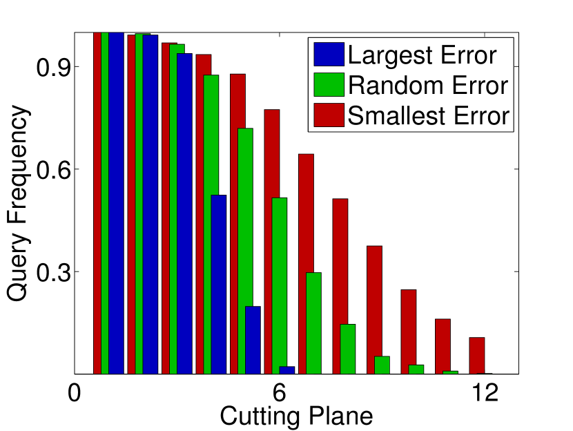
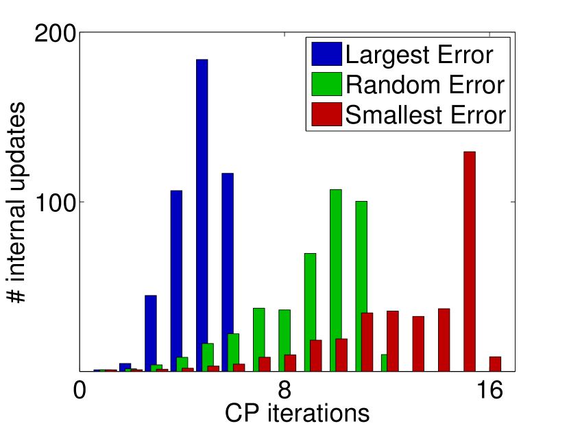
Figure 2: Left : for each value $i$ the bar represents the empirical probability (over $1,000$ runs) to query at least $i$ cutting planes. Right: each bar represents the number of internal Perceptron updates computed after each Cutting Plane loop.

The left pane of Figure 2 supports the soundness of our approach in the case of a compression scheme with no more than $6$ cutting planes for the best strategy (Largest Error). Additionally, we can observe a sharp decrease after the third cutting plane with this strategy and $80\%$ of the time, only $4$ cutting planes are required to model the dataset. In contrast, the right-hand side of Figure 2 reveals a trade-off between the number of cutting planes used and the number of internal updates for each cutting plane. We observe a smooth shift across our three strategies with Smallest Error putting the emphasis on small number of internal updates. In all respect, the Random Error strategy acts as a middle ground between the two other extreme approaches.

For the second experiment the margin (i.e. the volume of ${\cal W}$) is variable with values between $0.01$ and $0.3$. We also monitor the total number of internal updates rather than the per cutting plane value for the three strategies and a regular Perceptron Algorithm . Remind that this value is bounded from Proposition 2. This bound also holds for the regular Perceptron.

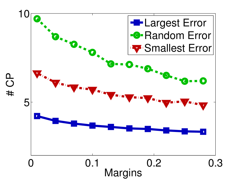
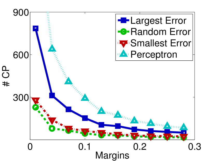
Figure 3: Left: The average number of cutting planes used for each strategy with respect to the value of $\gamma$. Right: the total number of internal updates with respect to $\gamma$. The fourth plot corresponds to a regular Perceptron

The previously observed behavioral shift across the three strategies is confirmed by Figure 3. Additionally, some relative robustness is observed with respect to $\gamma$, especially when the emphasis is put on querying a small number of cutting planes. It is interesting to note that the Random Strategy makes nearly as few updates as Smallest error while still querying a—relatively—low number of cutting planes. Finally, all three strategies are making slightly less updates than the regular Perceptron. To conclude, note that the theoretical bound of Proposition 2 is far too big to be plotted on the plot on the left of Figure 2.

IV-B Active Learning on Real Data

We illustrate our method for active learning on text classification data. For easy comparison, we follow an experimental procedure similar as the one in [1]. Namely, we use the Reuters-21578 —ModApte variation— and Newsgroups datasets. The Reuters dataset is composed of $8,293$ documents represented in TF-IDF form for $18,933$ words. The dataset spans $65$ topics such as Earn, Coffee or Cocoa and is split in $5,946$ training examples and $2,347$ test examples. On the other hand, the Newsgroups dataset accounts for $18,846$ documents of $26,214$ features splitted in $20$ topics. Half of this dataset is uniformly picked for training while the rest is kept for testing purposes. On both datasets we train a “one-versus-all” classifier for each class. We start by creating a pool of unlabeled training examples sampled from the training set. Then we run Algorithm 4. We use two variations of the Query() function: one based on the Chebyshev center (note that this is equivalent to the Active-SVM of [1]), and the other based on an approximation of the center of gravity from Minka’s Expectation Propagation method [34]. This last approach corresponds to the Active-BPM algorithm and has, to the best of our knowledge, never been used before. It is a direct application of Active Learning algorithms with Cutting planes method to the Bayes Point Machine. For both methods, we use two pools of different sizes ($500$ and $1,000$ examples). For initialization reasons, each pool comes with two already labeled vectors. All the computations are done with a linear kernel and the presented results are class-wise accuracy measurements on the test examples over the $10$ most represented classes. The values reported here are an average of these measures over $25$ runs. We complement these two datasets with Gunnar Raetsch’s Banana dataset. The Banana dataset is a widely used bataset of $2$-dimensionnal points split into two classes from which we extract $400$ training and $4900$ test examples. Due to its small size, the whole training set is used for the pool of unlabeled example. The computations are realized with an RBF kernel of parameter $\sigma=0.5$ and presented results are averaged over $50$ runs.

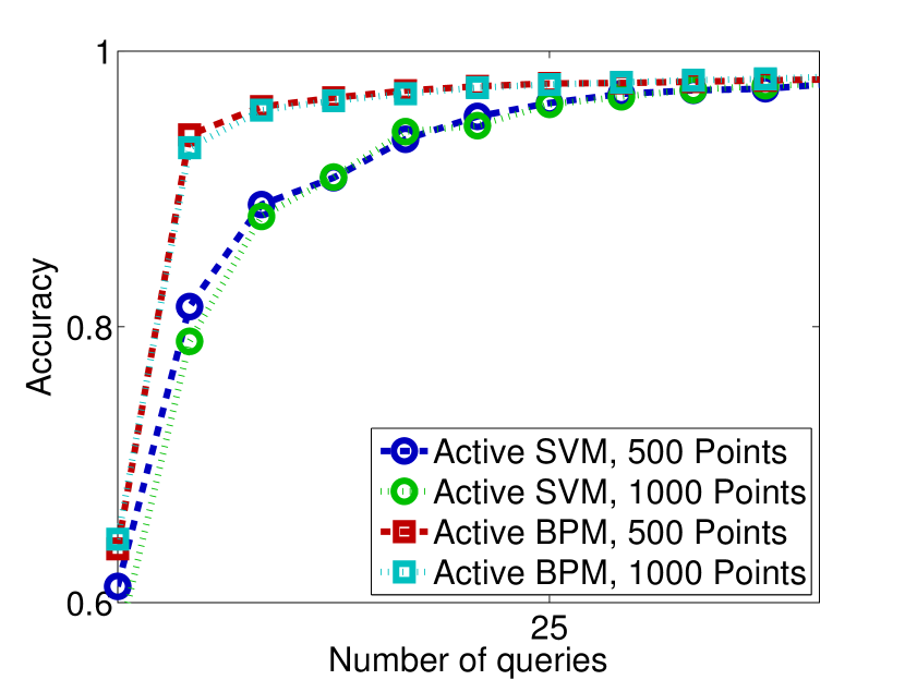
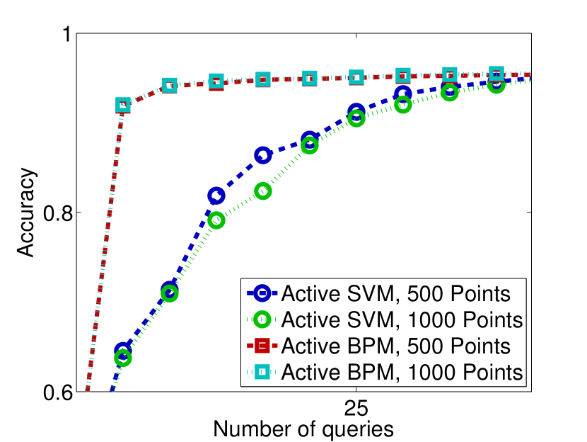
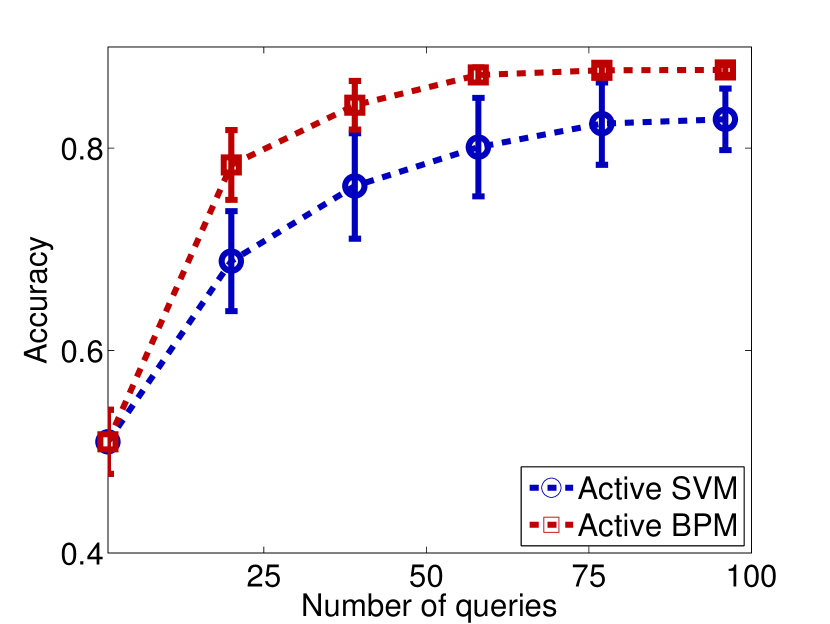
Figure 4: Accuracy on the Reuters (left) and Newsgroups (middle) datasets for Active-SVM and Active-BPM for pools of $500$ and $1000$ examples. Left: accuracy with error bars on the Banana dataset (Gunnar Raetsch) for Active-SVM and Active-BPM.

Figure 4 graphically depicts the behavior of the so-called Active-SVM [1] and the Active-BPM algorithms on each dataset. Namely, in both algorithms, the queries are selected according to their distance to the “centroid” of ${\cal C}$, which, in turn, serves as classifier. The difference between these two algorithms lies in that Active-SVM uses the Chebyshev center and Active-BPM the center of gravity for centroid. In Figure 4, data are represented by circles of squares whether they correspond to results achieved by Active-SVM or Active-BPM. Additionally, for the Reuters and Newgroups datasets, dashed plots correspond to the pool of $500$ examples while dotted plots relate to the pool of $1000$ examples. The error bounds on the third plot (Banana) correspond to the usual standard deviation. Each plot represents the accuracy of those algorithms with respect to the number of queries made. We can see that Active-BPM systematically outperforms Active-SVM and increases its accuracy faster for all datasets, already attaining an accuracy of $0.9$ after roughly $10$ queries for both Reuters and Newsgroups datasets. Both algorithm seem to stabilize after $30$ queries, with the Active-BPM being slightly more accurate than its SVM counterpart. For the Banana dataset, the accuracy increase in the first queries is a lot smoother, with an accuracy for Active-BPM of roughly $0.8$ after $20$ queries. Both algorithms seem to have converged after $60$ queries. Comparatively, not only does Active-BPM clearly dominate its SVM counterpart but it is also more stable as evidenced by the error bars which become negligible past the $60^{\text{th}}$ query.

V Conclusion and Future Directions

In this paper, we have shown that deep connections exist between Localization methods and Learning algorithms. Both fields have extensively characterized and studied similar concepts over the past years, sometime independently. On the other hand, complementary results have been found in each community. A notable example is the absence of a kernel approach in the Cutting Planes literature while center of gravity methods were mostly unknown in machine learning until Herbrich’s BPM [2]. We may also mention that the Cutting planes’ equivalent of the famous SVM [30] appears as soon as the $70$’s in [28]. This work is a testimony on how it is possible to derive new learning algorithms, both efficient and theoretically funded, by reformulating Cutting Planes approach for the learning paradigm. Besides the cutting plane-related flavor of the present work, it should be restated that Theorem 2 has a value that goes beyond the scope of this paper. A field that may be impacted by this result is obviously that of computational geometry where most of the results about the computation of centers of gravity come from; nonetheless, it should be noted that more closely related works could also benefit from our result. For instance, if we consider the active learning methods whose query steps rely on explicit exploration of all the possible query/label combinations (see, e.g. [36]), then Theorem 2 provides a tool to devise natural and theoretically sound heuristics to effectively locate the most informative query points, or, in other words, those that may lead to the smallest expected error.

Among all the possible extensions of this work, one we are particularly interested in is to study how these results may carry over to the multiclass setting and provide proper multiclass active algorithms based on, for example, Crammer’s Ultraconservative Additive Algorithms [37].

This appendix is composed of three sections. Section A serves as reminder of basic notions and results for the proofs of the other sections, additionally, we will introduce our set of notation thorough this section. Section B consists in a rewriting of the proof of Grunbaum in [24] on the partition of convex bodies by hyperplanes. The proof is restated in full with proper notation as it is the starting point of our result. The last section gives the proof of theorem 4 which is an extended version of the result of Grunbaum and is one of the contribution of our paper.

Appendix A Preliminaries

A-A Hyper-Sphere and Hyper-Ball

Definition 3 ($n$-dimensional Sphere).

We call $n$-sphere of center $O\in\mathbb{R}^{n}$ and radius $R\in\mathbb{R}$ and write $\mathcal{S}(O,R)\subset\mathbb{R}^{n}$ the subset

$$\mathcal{S}(O,R)\doteq\{x\in\mathbb{R}^{n}:\|x-O\|_{2}=R\}$$

Definition 4 ($n$-dimensional Ball).

We call $n$-ball of center $O\in\mathbb{R}^{n}$ and radius $R\in\mathbb{R}$ and write $\mathcal{B}(O,R)\subset\mathbb{R}^{n}$ the subset

$$\mathcal{B}(O,R)\doteq\{x\in\mathbb{R}^{n}:\|x-O\|_{2}<R\}$$

Alternatively, one can think of a ball as :

$$\mathcal{B}(O,R)\doteq\bigcup_{r\in[0,R]}\mathcal{S}(0,r)$$

Definition 5 (Surface of a spehe).

We call Surface of the $n$-sphere $\mathcal{S}(O,R)$ and write $\text{V}(\mathcal{S}(O,R))$ the $n-1$ dimensional volume

$$\text{V}(\mathcal{S}(O,R))\doteq\Pi^{s}_{n}\times R^{n-1}$$

Where $\Pi^{s}_{n}$ is a constant factor depending only on $n$ (e.g $\Pi^{s}_{1}=2$, $\Pi^{s}_{2}=2\pi$, $\Pi^{s}_{3}=4\pi$ and so on …)

Definition 6 (Volume of a Ball).

We call Volume of the $n$-ball $\mathcal{B}(O,R)$ and write $\text{V}(\mathcal{B}(O,R))$ the $n$-dimensional volume

$$\text{V}(\mathcal{B}(O,R))\doteq\int_{0}^{R}\text{V}(\mathcal{S}(O,r))dr$$

That is

$$\text{V}(\mathcal{B}(O,R)) =\int_{0}^{R}\Pi^{s}_{n}R^{n-1}dr$$

$$=\frac{\Pi^{s}_{n}R^{n}}{n}$$

$$=\Pi_{n}R^{n}$$

Where $\Pi_{n}\doteq\frac{\Pi^{s}_{n}}{n}$ is a constant factor depending only on $n$.

A-B Hyper-Cone

From these core definitions, we can now introduce (Hyper)-cones and some of their core properties. Intuitively, an Hyper-cone of dimension $n+1$, center $O$, radius $R$ and height $H$ is a sequence of $n$-Ball of linearly decreasing radius between $R$ and $0$, each one living on a difference “slice” of $\mathbb{R}^{n+1}$ between $O$ and $0+H$.

Remark 1.

We will use ${\bf v}_{n+1}$ to denote the vector of $\mathbb{R}^{n+1}$ with $1$ on its $n+1$ component and $0$ elsewhere.

Definition 7 (Hyper-cone).

We call Hyper-cone of dimension $n+1$, base $\mathcal{B}(O,R)\subset\mathbb{R}^{n}$ and height $H$ the set :

$$H\doteq\bigcup_{\forall h\in[0,H]}\mathcal{B}\left(O+h{\bf v}_{n+1},\frac{H-h}{H}R\right)$$

Alternatively, we can define the apex $Z\doteq O+H\times{\bf v}_{n+1}$ of the hyper-cone and give the following definition :

Definition 8 (Hyper-cone (2)).

We call Hyper-cone of dimension $n+1$, base $\mathcal{B}(O,R)\subset\mathbb{R}^{n}$ and apex $Z$ the convex hull $\textbf{conv}\left(\{\mathcal{B}(O,R);z\}\right)$.

We are now ready to state the core properties of Hyper-cone that we will use in the remaining of this document.

We start with the volume of a Hyper-cone

Definition 9 (Volume of Hyper-cone).

Given an Hyper-cone $C\in\mathbb{R}^{n+1}$ of dimension $n+1$, base $\mathcal{B}(O,R)\subset\mathbb{R}^{n}$ and height $H$ we call volume and write $\text{V}(C)$ the $n+1$-dimensional volume :

$$\text{V}(C)\doteq\int_{0}^{H}\text{V}\left(\mathcal{B}\left(O+h{\bf v}_{n+1},\frac{H-h}{H}R\right)\right)dh$$

Proposition 3.

The volume of the Hyper-cone $C\subset\mathbb{R}^{n+1}$ of dimension $n+1$, base $\mathcal{B}(O,R)\subset\mathbb{R}^{n}$ and height $H$ is

$$\text{V}(C)=\frac{\Pi_{n}R^{n}}{n+1}H$$

Proof.

From the definition of volume of a sphere we have $\text{V}(\mathcal{B}(O,R))\doteq\Pi_{n}R^{n}$. Substituting $R$ by $\frac{H-h}{R}$ and from the definition of the volume of a Hyper-cone we have

$$\text{V}(C)=\int_{0}^{H}\Pi_{n}\left(\frac{H-h}{H}R\right)^{n}dh$$

We substitute $h$ by $u\doteq H-h$, $du=-dh$.

$$\text{V}(C) =\int_{H}^{0}-\Pi_{n}\left(\frac{u}{H}R\right)^{n}du$$

$$=\int_{0}^{H}\Pi_{n}\left(\frac{u}{H}R\right)^{n}du$$

$$=\frac{\Pi_{n}R^{n}}{H^{n}}\int_{0}^{H}u^{n}du$$

$$=\frac{\Pi_{n}R^{n}}{H^{n}}\times\frac{H^{n+1}}{n+1}$$

$$=\frac{\Pi_{n}R^{n}}{n+1}H$$

∎

A-C Center of Mass

With the previous definition formally stated, we can now go one step further and define the center of mass or sometimes called center of gravity

Definition 10 (Center of gravity).

For a given convex body $X\subset\mathbb{R}^{n}$ we call center of gravity and write $\textbf{cg}(X)\in\mathbb{R}^{n}$ the point :

$$\textbf{cg}(X)=\frac{1}{\text{V}(X)}\int_{x\in X}xdx$$

Proposition 4.

Let $S$ a $n$-dimensional sphere such that $S\doteq\mathcal{S}(O,R)$. Then $\textbf{cg}(S)=O$.

Proof.

Without loss of generality, assume that $O=0$. Then, $S=\{x\in\mathbb{R}^{n}:\|x\|_{2}=R\}$. Since $\|x\|_{2}=\|-x\|_{2}$ it is clear that $\forall x\in\mathbb{R}^{n}:x\in S\Leftrightarrow-x\in S$. Thus, we can rewrite $\textbf{cg}(S)$ as

$$\textbf{cg}(S)=\frac{1}{\text{V}(S)}\int_{x\in S}-xdx$$

Thus

$$2\textbf{cg}(S) =\frac{1}{\text{V}(S)}\left(\int_{x\in S}xdx+\int_{x\in S}-xdx\right)$$

$$=\frac{1}{\text{V}(S)}\int_{x\in S}x-xdx$$

$$=0$$

∎

Proposition 5.

Let $B$ a $n$-dimensional ball such that $B\doteq\mathcal{B}(O,R)$. Then $\textbf{cg}(B)=O$.

Proof.

Remind that $B$ can be seen as a collection of concentric $n$-sphere of center $O$ and radii between $0$ and $R$ (see Def. 4). Then, we can rewrite $\textbf{cg}(B)$ as

$$\textbf{cg}(B) =\frac{1}{\text{V}(B)}\int_{0}^{R}\textbf{cg}(\mathcal{S}(O,r))\text{V}(\mathcal{S}(O,r))dr$$

$$=O$$

Where the last line come from Proposition 4. ∎

Proposition 6 (Center of Gravity of an Hyper-cone).

Let $C$ a $n+1$ dimensional Hyper-cone ($C\subset\mathbb{R}^{n+1}$) of base $\mathcal{B}(O,R)\subset\mathbb{R}^{n}$ and apex $Z$ such that $\|Z-O\|_{2}=H$. Then, $\textbf{cg}(C)$ is located on the segment $[O;Z]$ at a distance $H/_{n+2}$ of $O$.

Proof.

Without loss of generality, we assume that $O=0$ and $Z=H{\bf v}_{n+1}$. By definition, $C$ is a collection of ball, and we can rewrite $\textbf{cg}(C)$ as :

$$\textbf{cg}(C)=\frac{1}{\text{V}(C)}\int_{0}^{H}\textbf{cg}\left[\mathcal{B}\left(h{\bf v}_{n+1},\frac{H-h}{H}R\right)\right]\times\text{V}\left[\mathcal{B}\left(h{\bf v}_{n+1},\frac{H-h}{H}R\right)\right]dh$$

From Proposition 5 it is clear that $\textbf{cg}(C)$ lies on the segment $[O;Z]$. The remaining of the proof came by explicitly calculating $\textbf{cg}(C)$.

$$\textbf{cg}(C) =\frac{1}{\text{V}(C)}\int_{0}^{H}h{\bf v}_{n+1}\times\text{V}\left[\mathcal{B}\left(h{\bf v}_{n+1},\frac{H-h}{H}R\right)\right]dh$$ (Prop. 5)

$$=\frac{1}{\text{V}(C)}\int_{0}^{H}h{\bf v}_{n+1}\frac{\Pi_{n}R^{n}}{H^{n}}(H-h)^{n}dh$$ (Volume of a Ball)

$$=\frac{1}{\text{V}(C)}\int_{0}^{H}(H-u){\bf v}_{n+1}\frac{\Pi_{n}R^{n}}{H^{n}}u^{n}du u\doteq H-h$$ (Subst. , see Prop. 3)

$$=\frac{1}{\text{V}(C)}\left[\int_{0}^{H}\frac{\Pi_{n}R^{n}H{\bf v}_{n+1}}{H^{n}}u^{n}du-\int_{0}^{H}\frac{\Pi_{n}R^{n}{\bf v}_{n+1}}{H^{n}}u^{n+1}du\right]$$

$$=\frac{1}{\text{V}(C)}\left[\frac{\Pi_{n}R^{n}{\bf v}_{n+1}}{H^{n-1}}\int_{0}^{H}u^{n}du-\frac{\Pi_{n}R^{n}{\bf v}_{n+1}}{H^{n}}\int_{0}^{H}u^{n+1}du\right]$$

$$=\frac{1}{\text{V}(C)}\left[\frac{\Pi_{n}R^{n}H^{n+1}{\bf v}_{n+1}}{H^{n-1}(n+1)}-\frac{\Pi_{n}R^{n}H^{n+2}{\bf v}_{n+1}}{H^{n}(n+2)}\right]$$

$$=\frac{1}{\text{V}(C)}\left[\frac{\Pi_{n}R^{n}H^{2}{\bf v}_{n+1}}{n+1}-\frac{\Pi_{n}R^{n}H^{2}{\bf v}_{n+1}}{n+2}\right]$$

$$=\frac{n+1}{\Pi_{n}R^{n}H}\left[\frac{\Pi_{n}R^{n}H^{2}{\bf v}_{n+1}}{n+1}-\frac{\Pi_{n}R^{n}H^{2}{\bf v}_{n+1}}{n+2}\right]$$ (Volume of a Hyper-cone)

$$=\left(H-H\frac{n+1}{n+2}\right){\bf v}_{n+1}$$

$$=\left(1-\frac{n+1}{n+2}\right)H{\bf v}_{n+1}$$

$$=\left(\frac{n+2-n-1}{n+2}H{\bf v}_{n+1}\right)$$

$$=\left(\frac{H}{n+2}\right){\bf v}_{n+1}$$

That is to say, $\textbf{cg}(C)$ is on the segment $[O;Z]$ at a distance $H/_{n+2}$ of $O$.

∎

A-D Hyperplane and Halfspace

Definition 11.

We call ($n$)-Hyperplane of normal $w\in\mathbb{R}^{n}$ and offset $b\in\mathbb{R}$ and write $W(w,b)\subset\mathbb{R}^{n}$ the subset :

$$W(w,b)\doteq\{x\in\mathbb{R}^{n}:\left<{w},{x}\right>+b=0\}$$

Definition 12.

We call Positive Halfspace of the $n$-Hyperplane $W(w,b)\subset\mathbb{R}^{n}$ and write $W^{+}(w,b)\subset\mathbb{R}^{n}$ the subset

$$W^{+}(w,b)\doteq\{x\in\mathbb{R}^{n}:\left<{w},{x}\right>+b\geq 0\}$$

Conversely, we call Negative Halfspace of $W(w,b)\subset\mathbb{R}^{n}$ and write $W^{-}(w,b)\subset\mathbb{R}^{n}$ the subset

$$W^{-}(w,b)\doteq\{x\in\mathbb{R}^{n}:\left<{w},{x}\right>+b\leq 0\}$$

Additionally, note that $W(w,b)\subset W^{+}(w,b)$ but $W(w,b)\not\subset W^{-}(w,b)$.

Definition 13.

For any subset $X\subset\mathbb{R}^{n}$ and any Hyperplane $W\subset\mathbb{R}^{n}$ we call Positive Partition and write $X^{+}\subset\mathbb{R}^{n}$ the subset

$$X^{+}\doteq X\cap W^{+}$$

Conversely, for we call Negative Partition and write $X^{-}\subset\mathbb{R}^{n}$ the subset

$$X^{-}\doteq X\cap W^{-}$$

Proposition 7 (Volume reduction of Hyper-Cone).

For any $(n+1)$-Hyper-cone of base $\mathcal{B}(O,R)$, apex $Z$ and Height $H$, let set $W_{\textbf{cg}(C)}\doteq W({\bf v}_{n+1},H/_{n+2})$ the Hyperplane passing by $\textbf{cg}(C)$ ( i.e. $\textbf{cg}(C)\in W_{\textbf{cg}(C)}$ ) and parallel to $\mathbb{R}^{n}$. Then,

$$\text{V}(C^{+})=\text{V}(C)\left[\frac{1}{\left(1+\frac{1}{n+1}\right)^{n+1}}\right]\geq\text{V}(C)e^{-1}$$

Proof.

We start by proving the right-hand side of the relation. Let set $n^{\prime}=n+1$ and divide both side by $\text{V}(C)$ then we can rewrite it as

$$\frac{1}{\left(1+\frac{1}{n^{\prime}}\right)^{n^{\prime}}}\geq e^{-1}$$

From the usual definition of $e$ we have that

$$\lim_{n\rightarrow\infty}\left(1+\frac{1}{n^{\prime}}\right)^{n^{\prime}}=e$$

$$\Leftrightarrow \lim_{n^{\prime}\rightarrow\infty}\frac{1}{\left(1+\frac{1}{n^{\prime}}\right)^{n^{\prime}}}=e^{-1}$$

And by standard arguments we can show that

$$\frac{1}{\left(1+\frac{1}{n^{\prime}}\right)^{n^{\prime}}}\geq\frac{1}{\left(1+\frac{1}{n^{\prime}+1}\right)^{n^{\prime}+1}}$$

Therefore

$$\frac{1}{\left(1+\frac{1}{n^{\prime}}\right)^{n^{\prime}}}\geq\lim_{n\rightarrow\infty}\frac{1}{\left(1+\frac{1}{n^{\prime}}\right)^{n^{\prime}}}=e^{-1}$$

Finally, the left-hand side of relation is obtained by direct calculation of $\text{V}(C+)$. The general idea is the same than the calculation of $\text{V}(C)$ but, instead of integrating over the entire height we start at $H/_{n+2}$, thus ignoring $C^{-}$. Besides, without loss of generality, we assume that $O=0$ and that $Z=H{\bf v}_{n+1}$.

$$\text{V}(C^{+}) =\int_{H/_{n+2}}^{H}\text{V}\left[\mathcal{B}\left(h{\bf v}_{n+1},\frac{H-h}{H}R\right)\right]dh$$

$$=\int_{H/_{n+2}}^{H}\Pi_{n}\frac{R^{n}}{H^{n}}(H-h)^{n}dh$$ (Volume of a Ball)

$$=\int_{0}^{H\left(1-\frac{1}{n+2}\right)}\Pi_{n}\frac{R^{n}}{H^{n}}u^{n}du u\doteq H-h$$ (Subst. )

$$=\frac{\Pi_{n}R^{n}}{H^{n}}\int_{0}^{H\left(1-\frac{1}{n+2}\right)}u^{n}du$$

$$=\frac{\Pi_{n}R^{n}}{H^{n}}\times\frac{H^{n+1}}{n+1}\times\left(1-\frac{1}{n+2}\right)^{n+1}$$

$$=\frac{\Pi_{n}R^{n}H}{n+1}\times\left(1-\frac{1}{n+2}\right)^{n+1}$$

$$=\text{V}(C)\left(1-\frac{1}{n+2}\right)^{n+1}$$

$$=\text{V}(C)\left(\frac{n+1}{n+2}\right)^{n+1}$$

$$=\text{V}(C)\left(\frac{(n+1)\times\frac{1}{n+1}}{(n+2)\times\frac{1}{n+1}}\right)^{n+1}$$

$$=\text{V}(C)\left(\frac{1}{\frac{n+2}{n+1}}\right)^{n+1}$$

$$=\text{V}(C)\left(\frac{1}{1+\frac{1}{n+1}}\right)^{n+1}$$

$$=\text{V}(C)\left[\frac{1}{\left(1+\frac{1}{n+1}\right)^{n+1}}\right]$$

∎

A-E Setting

For the remaining of this document, let $K$ be a (full dimensional) convex body in $\mathbb{R}^{n+1}$.

Definition 14.

For any convex body $K\in\mathbb{R}^{n+1}$ we say that $K$ is Spherically Symmetric along the unit vector ${\bf v}$ if and only if $\forall\lambda\in\mathbb{R}$ the cut of $K$ by the hyperplane $W({\bf v},\lambda)$ (i.e. $K\cap W({\bf v},\lambda)$) is a $n$ dimensional hypersphere of center $\lambda{\bf v}$

Appendix B Partition of Convex Bodies By Hyper-Plane

This section consists in a rewriting of the proof of [24] instantiated within the previously defined notation and setting.

B-A Theorem

Theorem 3.

For any convex body $K\subset\mathbb{R}^{n+1}$, and any hyperplane $W$. If $\textbf{cg}(K)\in K^{+}$ then

$$\text{V}(K^{+})\geq e^{-1}\times\text{V}(K)$$

Proof.

Note 1 (Points along ${\bf v}_{n+1}$).

This proof will revolve around key points located on the $n+1^{\text{th}}$ axis of $\mathbb{R}^{n+1}$ of base vector ${\bf v}_{n+1}$. In an attempt to avoid overburdening the notation, we will treat these points as number along the real line when context is clear. Therefore, if $x=\lambda_{1}{\bf v}_{n+1}$ and $y=\lambda_{2}{\bf v}_{n+1}$ we will freely write $x>y$ if $\lambda_{1}>\lambda_{2}$.

Let $W$ the hyperplane such that $W=\arg\min_{W}\text{V}(K^{+})$ such that $\textbf{cg}(K)\in K^{+}$. It is easy to see that $\textbf{cg}(K)\in W$ : if $\textbf{cg}(K)\notin W$ you can always reduce $\text{V}(K^{+})$ by shifting $W$ toward $\textbf{cg}(K)$. Without loss of generality, let’s say that $\textbf{cg}(K)=0$ the origin of $\mathbb{R}^{n+1}$ and that ${\bf v}_{n+1}$ is the normal vector of $W$ with $b=0$, hence $W=W({\bf v}_{n+1},0)$.

In order to ease the comprehension of the proof, we make the following assumption that we will lift later on.

Assumption 1.

$K$ is a convex body which is Spherically Symmetric along ${\bf v}_{n+1}$

A direct implication of this is that $\textbf{cg}(K)=\textbf{cg}(K\cap W)$. In other words, $\textbf{cg}(K)$ is the center of the $n-1$ dimensional sphere $K\cap W$ (see, for example, the argument of Prop. 6 ).

Let $C^{+}$ the Hyper-cone of base $K\cap W$ and apex $Z$ such that $C^{+}\subset W^{+}$ and $\text{V}(C^{+})=\text{V}(K^{+})$.

Moreover either :

• $K^{+}=C^{+}$ and $Z$ is the apex of $K^{+}$

• $Z\notin K^{+}$

To prove that, remember that each slice $K\cap W({\bf v}_{n+1},\lambda)$ of $K$ along the $n+1$ axis is a sphere. We look at the function $r_{C^{+}}()$ (resp. $r_{K^{+}}()$) which maps each value of $\lambda\in\mathbb{R}_{+}$ with the radius of the corresponding slice of $C^{+}$ (resp. $K^{+}$).By construction, we know that $r_{C^{+}}(0)=r_{K^{+}}(0)$ and, by definition $r_{C^{+}}()$ is a deacreasing linear function. If $r_{K^{+}}()$ has any stricly convex part, then there exists an arc $[r_{K^{+}}(\lambda_{1}),r_{K^{+}}(\lambda_{2})]$ which is not in $K^{+}$ and therefore $K$ is not a convex set. Therefore $r_{K^{+}}()$ is concave. Then, because $r_{C^{+}}(0)=r_{K^{+}}(0)$, for $Z$ to be in $K^{+}$ either $K^{+}$ is a Hyper-cone (and $r_{K^{+}}$ is linear) or $\text{V}(K^{+})>\text{V}(C^{+})$ (that is to say $\int_{0}^{\infty}r_{K^{+}}(\lambda)d\lambda>\int_{0}^{\infty}r_{C^{+}}(\lambda)d\lambda$ ) which is in contradiction with the definition of $C^{+}$

As a consequence, $C^{+}$ is at least as elongated as $K^{+}$. In other words, the mass of $C^{+}$ is more spread along the axis of ${\bf v}_{n+1}$, this incurs a shift of the center of gravity of $\textbf{cg}(C^{+})$ with respect to $\textbf{cg}(K^{+})$. Therefore $\textbf{cg}(C^{+})$ is on the closed segment $\left[\textbf{cg}(K^{+}),Z\right]$.

Thus, by using the notation introduced in Note 1 :

$$0=\textbf{cg}(K)\leq\textbf{cg}(K^{+})\leq\textbf{cg}(C^{+})\leq Z$$

We now define $C^{-}$ by extending $C^{+}$ such that $C\doteq C^{-}\cup C^{+}$ is a cone of apex $Z$ and $\text{V}(C^{-})=\text{V}(K^{-})$. Therefore,

$$\text{V}(C) =\text{V}(C^{+})+\text{V}(C^{-})$$

$$=\text{V}(K^{+})+\text{V}(K^{-})$$

$$=\text{V}(K)$$

Once again, we are interested in the relative position of $\textbf{cg}(K^{-})$ and $\textbf{cg}(C^{-})$. We invoke the same arguments than before and claim that, in a similar way :

$$\textbf{cg}(K^{-})\leq\textbf{cg}(C^{-})\leq 0=\textbf{cg}(C)$$

Remark 2.

The proof for this is a little more tricky this time though. Part of this is due to the fact that $C^{-}$ is not a Hyper-cone in itself and one must consider $C$ and $K$ in their entirety for the nonconvexity argument. A possible start is to consider the radius increase along the reverse axis $\overline{{\bf v}_{n+1}}\doteq-{\bf v}_{n+1}$ and replicate the previous argument with added attention to the slope of $r_{K^{-}}()$ which must be such that $r_{K}()$ as a whole is still concave.

Let $\alpha,\beta\in\mathbb{R}$ such that $\alpha\doteq{\text{V}(K^{+})}/_{\text{V}(K)}$ and $\beta\doteq{\text{V}(K^{-})}/_{\text{V}(K)}$. Then

$$\textbf{cg}(K)=\alpha\textbf{cg}(K^{+})+\beta\textbf{cg}(K^{-})$$

Or alternatively, by construction of $C$

$$\textbf{cg}(C)=\alpha\textbf{cg}(C^{+})+\beta\textbf{cg}(C^{-})$$

Combining these with the previous inequalities, we have that

$$\textbf{cg}(K)\leq\textbf{cg}(C)$$

Moreover, we know from Proposition 6 that $\textbf{cg}(C)$ is at a distance $H/_{n+2}$ of its base, where $H$ is the height of $C$.

Let $\widetilde{W}\doteq W({\bf v}_{n+1},\tilde{b})$ such that $\textbf{cg}(C)\in\widetilde{W}$ and write $\widetilde{C^{+}}$ the positive partition of $C$ by $\widetilde{W}$, that is $\widetilde{C^{+}}\doteq\widetilde{W^{+}}\cap C$.

From Proposition 7 we have that $\text{V}\left(\widetilde{C^{+}}\right)\geq e^{-1}\text{V}(C)$. Moreover, because of $\textbf{cg}(C)\geq\textbf{cg}(K)$ we have that $\text{V}(C^{+})\geq\text{V}\left(\widetilde{C^{+}}\right)$.

Putting all of this together we get that

$$\text{V}(K^{+}) =\text{V}(C^{+})$$

$$\geq\text{V}\left(\widetilde{C^{+}}\right)$$

$$\geq e^{-1}\text{V}(C)$$

$$=e^{-1}\text{V}(K)$$

Finally, all we have left is to deal with Assumption 1. This is simply tackled by remarking that, by definition, spherical symmetrization preserve volumes along its axis. Thus, for any $K$ of any convex shape it suffices to apply the proof on the spherical symmetrization of $K$ : $\textbf{sym}_{S}(K)$ and we have

$$\text{V}(K^{+})=\text{V}(\textbf{sym}_{S}(K^{+}))\geq e^{-1}\text{V}(\textbf{sym}_{S}(K))=\text{V}(K)$$

∎

Appendix C Generalized Volume Reduction

This section is dedicated to the main theorem which is a generalization of Theorem 3 to approximate center of mass.

Theorem 4.

For any convex body $K\subset\mathbb{R}^{n+1}$ and any Hyper-plane $W$ of normal ${\bf v}$, splitting $K$ in $K^{+}$ and $K^{-}$. Let

$$X\doteq\textbf{cg}(K)+\lambda\frac{(n+1)\text{V}(K)}{\Pi_{n}R_{K^{+}}^{n}}\left[\frac{H_{K^{+}}}{(n+2)H_{K^{-}}}\right]^{n}\left[1-\frac{1}{n+2}\right]{\bf v}$$

Where $H_{K^{+}}=\max_{a\in K^{+}}a^{T}{\bf v}$, $H_{K_{-}}=\min_{a\in K^{-}}a^{T}{\bf v}$ and $R_{K^{+}}$ the radius of the $n-1$-Ball $\mathcal{B}_{K\cap W}$ such that $\text{V}(\mathcal{B}_{K\cap W})=\text{V}(K\cap W)$.

Then, if $X\in K^{+}$ the following holds true

$$\text{V}(K^{+})\geq\text{V}(K)(1-\lambda)^{n+1}e^{-1}$$

Proof.

The proof start in a similar way than the one of Grunbaum, with respect to $X$.

Namely, let Assumption 1 hold for now, and let $W$ the hyperplane such that $W=\arg\min_{W}\text{V}(K^{+})$ such that $X\in K^{+}$. Same as before, we have that $X\in W$. Without loss of generality, let’s say that $X=0$ the origin of $\mathbb{R}^{n+1}$ and that ${\bf v}_{n+1}$ is the normal vector of $W$ with $b=0$, hence $W=W({\bf v}_{n+1},0)$.

Let define $C^{+}$ the Hyper-cone of base $K\cap W$, apex $Z$ such that $C^{+}\subset W^{+}$ and $\text{V}(C^{+})=\text{V}(K^{+})$. Moreover, let $C^{-}$ the extension of $C^{+}$ such that $C\doteq C^{-}\cap C^{+}$ is an Hyper-cone of height $H$ and volume $\text{V}(C)=\text{V}(K)$. That is to say $\text{V}(C^{-})=\text{V}(K^{-})$. From the same argument than before, we know that $\textbf{cg}(C^{+})$ (resp. $\textbf{cg}(C^{-})$) is shifted with respect to $\textbf{cg}(K^{+})$ (resp. $\textbf{cg}(K^{-})$), thus, according to the notation defined in Note 1 we have that

$$\textbf{cg}(K)\leq\textbf{cg}(C)$$

If $X\leq\textbf{cg}(C)$ then the exact same argument than the one of Section B applies and

$$\text{V}(K^{+})\geq\text{V}(K)e^{-1}$$

Otherwise, we have that

$$\textbf{cg}(K)\leq\textbf{cg}(C)\leq X$$

The idea of the proof is to find $\widetilde{X}$ such that $X\leq\widetilde{X}$ from which we can bound the volume of $K^{+}$ in a similar way than before.

Let define

$$\widetilde{X}\doteq\textbf{cg}(C)+\lambda H\left[1-\frac{1}{n+1}\right]{\bf v}_{n+1}$$ (16)

Denote by $\mathcal{B}_{0}=\mathcal{B}(B_{0},R)$ the base of $C$ and remind that $C$ has height $H$ and apex $Z$ and remind that $\textbf{cg}(C)=B_{0}+H/_{n+2}{\bf v}{n+1}$. Therefore

$$\widetilde{X}=H\left[\lambda\left(1-\frac{1}{n+2}\right)+\frac{1}{n+2}\right]{\bf v}_{n+1}$$

Consider $\widetilde{W}\doteq W({\bf v}_{n+1},\widetilde{b})$ the Hyperplane of normal vector ${\bf v}_{n+1}$ (i.e. $\widetilde{W}$ is parallel to $W$) and offset $\widetilde{b}$ such that $\widetilde{X}\in\widetilde{W}$. Then, let $\widetilde{C^{+}}$ the positive partition of $C$ with respect to $\widetilde{W}$

$$\widetilde{C^{+}}=C\cap\widetilde{W^{+}}$$

We can compute the volume of $\widetilde{C^{+}}$ as follow :

$$\text{V}(\widetilde{C^{+}}) =\int_{\widetilde{X}}^{H}\text{V}\left[\mathcal{B}\left(B_{0}+h{\bf v}_{n+1},\frac{H-h}{H}R\right)\right]dh$$

$$=\int_{\widetilde{X}}^{H}\Pi_{n}\frac{R^{n}}{H^{n}}(H-h)^{n}dh$$ (Volume of a Ball)

$$=\int^{H-H\left[\lambda\left(1-\frac{1}{n+2}\right)+\frac{1}{n+2}\right]}_{0}\Pi_{n}\frac{R^{n}}{H^{n}}u^{n}du u\doteq H-h$$ (Subst. )

$$=\frac{\Pi_{n}R^{n}}{H^{n}}\int^{H(1-\lambda)\left[1-\frac{1}{n+2}\right]}_{0}u^{n}du$$

$$=\frac{\Pi_{n}R^{n}}{H^{n}}\times\frac{H^{n+1}}{n+1}(1-\lambda)^{n+1}\left[1-\frac{1}{n+2}\right]^{n+1}$$

$$=\text{V}(C)(1-\lambda)^{n+1}\left[1-\frac{1}{n+2}\right]^{n+1}$$ (Volume of a Hyper-cone)

$$\geq\text{V}(C)(1-\lambda)^{n+1}e^{-1}$$ (See Prop. 7)

Where in the first two lines, we allow a slight abuse of notation and use $\widetilde{X}$ as a real as explained in Note 1.

Then, we can rewrite the volume of $C^{+}$ as

$$\text{V}(C^{+})=\int_{X}^{\widetilde{X}}\text{V}\left[\mathcal{B}\left(B_{0}+h{\bf v}_{n+1},\frac{H-h}{H}R\right)\right]dh+\text{V}(\widetilde{C^{+}})$$

Consequently, if $X\leq\widetilde{X}$ then the first term of $\text{V}(C^{+})$ is positive and therefore, $\text{V}(C^{+})\geq\text{V}(\widetilde{C+})$

$$\widetilde{X} =\textbf{cg}(C)+\lambda H\left[1-\frac{1}{n+2}\right]$$

$$=\textbf{cg}(C)+\lambda\frac{(n+1)\text{V}(C)}{\Pi_{n}R^{n}}\left[1-\frac{1}{n+2}\right]$$ (Volume of a Hyper-cone)

$$\geq\textbf{cg}(K)+\lambda\frac{(n+1)\text{V}(K)}{\Pi_{n}R^{n}}\left[1-\frac{1}{n+2}\right] \textbf{cg}(C)\geq\textbf{cg}(K) \text{V}(C)=\text{V}(K)$$ ( and )

Unfortunately, we cannot easily compute $R$ directly. Nonetheless, since $\mathcal{B}_{0}$ and $W$ are parallel, we can use the Trianngle proportionality theorem. Denote $R_{C^{+}}$ the radius of the base of $C^{+}$, that is $K\cap W$ and $H_{C^{+}}$ the height of $C^{+}$ (i.e. the distance between $X$ and $Z$) then we have :

$$\frac{1}{R}=\frac{H_{C^{+}}}{HR_{C^{+}}}$$

From this, we want to bound $H_{C^{+}}$ and $H$ since $R_{C^{+}}$ is easy enough to estimate because it is directly related to $K$ and $W$.

From previous argument, we know that $Z\notin K^{+}$ except if $K^{+}=C^{+}$. So let define

$$H_{K^{+}}\doteq\max_{a\in K^{+}}a^{T}{\bf v}_{n+1}$$

Intuitively, $H_{K^{+}}$ is maximal distance between a point in $K^{+}$ and $X$ with respect to the axis of ${\bf v}_{n+1}$. Because $Z$ is precisely on this axis, and that $Z\notin K^{+}$ (or $K^{+}=C^{+}$) the following holds true

$$H_{K^{+}}\leq H_{C^{+}}$$ (17)

Conversly, let define $H_{K^{-}}$ as the maximal distance between $X$ and any point of $K^{-}$ with respect to the axis of ${\bf v}_{n+1}$. Again, from previous argument, we know that $B_{0}\in K^{-}$. Note that, because $C$ is a Hyper-cone, we know that $B_{0}$ is at a distance $H/_{n+2}$ of $\textbf{cg}(C)$. Moreover, remind that we are treating the case where $X\geq\textbf{cg}(C)$, hence, the distance between $B_{0}$ and $X$ is at least $H/_{n+2}$ which in turn is smaller than $H_{K^{-}}$. Reordering gives the following

$$H_{K^{-}} \geq\frac{H}{n+2}$$

$$\Leftrightarrow(n+2)H_{K^{-}} \geq H$$ (18)

Putting back equations $\eqref{eq:Hkp}$ and $\eqref{eq:Hkm}$ together, we have that

$$\frac{1}{R}\geq\frac{H_{K^{+}}}{(n+2)H_{K^{-}}R_{C^{+}}}$$

Which we plug back into the previous calculation

$$\widetilde{X} \geq\textbf{cg}(K)+\lambda\frac{(n+1)\text{V}(K)}{\Pi_{n}R^{n}}\left[1-\frac{1}{n+2}\right]$$

$$\geq\textbf{cg}(K)+\lambda\frac{(n+1)\text{V}(K)}{\Pi_{n}R_{C^{+}}^{n}}\left[\frac{H_{K^{+}}}{(n+2)H_{K^{-}}}\right]^{n}\left[1-\frac{1}{n+2}\right]$$

$$=X$$

Remind that we drop ${\bf v}_{n+1}$ in the above since we treat $\widetilde{X}$ and $X$ as real numbers (see Note 1).

To conlude this proof by rewinding all together. Namely,

• $X\leq\textbf{cg}(C)$ and

  $$\text{V}(K^{+})\geq\text{V}(K)e^{-1}$$

• $X\geq\textbf{cg}(C)$ and we can define $\widetilde{(}X)$ such that

  $$\text{V}(K^{+})\geq\text{V}(\widetilde{C^{+}})\geq\text{V}(K)(1-\lambda)^{n}e^{-1}$$

Once again, we lift Assumption 1 as before by noting that spherical symetry preserves volumes. One difference though lies in the fact that computing $R_{C^{+}}$ is no longer immediate in the general case. Notwithstanding, it can be easily approximated within satisfactory precision.

As a final note, we may mention that distinguishing between these two cases is non-trivial. Hence, without additionnal computation, only the worst bound can be guaranteed. ∎

References

- [1] S. Tong and D. Koller, “Svm active learning with applications to text classification,” JMLR, 2002.
- [2] T. G. R. Herbrich and C. Campbell, “Bayes point machines,” JMLR, 2001.
- [3] Y. Freund and R. E. Schapire, “Large margin classification using the perceptron algorithm,” Machine learning, 1999.
- [4] J.-L. Goffin, “The relaxation method for solving systems of linear inequalities,” Mathematical Operations Research, 1980.
- [5] T. S. Motzkin and I. J. Schoenberg, “The relaxation method for linear inequalities,” Canadian Journal of Mathematics, 1954.
- [6] H. Block, “The perceptron: a model for brain functioning,” Reviews of Modern Physics, 1962.
- [7] A. Novikoff, “On convergence proofs on perceptrons,” in Proceedings of the Symposium on the Mathematical Theory of Automata, 1962.
- [8] F. Rosenblatt, “The perceptron: A probabilistic model for information storage and organization in the brain,” Psychological Review, 1958.
- [9] S. Floyd and M. Warmuth, “Sample compression, learnability, and the vapnik-chervonenkis dimension,” Machine Learning, 1995.
- [10] T. Joachims, T. Finley, and C.-N. Yu, “Cutting-plane training of structural svms,” Machine Learning, 2009.
- [11] V. Franc and S. Sonnenburg, “Optimized cutting plane algorithm for large-scale risk minimization,” JMLR, 2009.
- [12] C. H. Teo, S. V. N. Vishwanathan, A. J. Smola, and Q. V. Le, “Bundle methods for regularized risk minimization.” JMLR, 2010.
- [13] B. Settles, “Active learning,” in Synthesis Lectures on Artificial Intelligence and Machine Learning, 2012.
- [14] D. Golovin and A. Krause, “Adaptive submodularity: A new approach to active learning and stochastic optimization,” CoRR, 2010.
- [15] A. Gonen, S. Sabato, and S. Shalev-Shwartz, “Efficient active learning of halfspaces: an aggressive approach,” JMLR, 2013.
- [16] M. F. Balcan, A. Broder, and T. Zhang, “Margin based active learning,” in COLT, 2007.
- [17] D. D. Lewis and W. A. Gale, “A sequential algorithm for training text classifiers,” in Proceedings of the 17th annual international ACM SIGIR conference on Research and development in information retrieval. Springer-Verlag New York, Inc., 1994, pp. 3–12.
- [18] J. E. Kelley, “The cutting plane method for solving convex programs,” SIAM, 1960.
- [19] Y. Nesterov, “Cutting plane algorithms from analytic centers: efficiency estimates,” Mathematical Programming, 1995.
- [20] F. Dabbene, P. S. Shcherbakov, and B. T. Polyak, “A randomized cutting plane method with probabilistic geometric convergence.” SIAM Journal on Optimization, 2010.
- [21] T. Graepel, R. Herbrich, and J. Shawe-Taylor, “PAC-Bayesian Compression Bounds on the Prediction Error of Learning Algorithms for Classification,” Machine Learning, 2005.
- [22] Y. Li, H. Zaragoza, R. Herbrich, J. Shawe-Taylor, and J. Kandola, “The perceptron algorithm with uneven margins,” 2002.
- [23] K. Crammer, O. Dekel, J. Keshet, S. Shalev-Shwartz, and Y. Singer, “Online passive-aggressive algorithms,” JMLR, 2006.
- [24] B. Grunbaum, “Partitions of mass-distributions and of convex bodies by hyperplanes,” Pacific Journal of Mathematics, 1960.
- [25] D. J. Newman, “Location of the maximum on unimodal surfaces,” J. ACM, 1965.
- [26] A. Levin, “On an algorithm for the minimization of convex functions,” Soviet Math. Doklady, 1965.
- [27] S. Boyd and L. Vandenberghe, “Localization and cutting-plane methods,” 2008.
- [28] J. Elzinga and T. G. Moore, “A central cutting plane algorithm for the convex programming problem,” Mathematical Programming, 1975.
- [29] S. P. Boyd and L. Vandenberghe, Convex optimization, 2004.
- [30] V. N. Vapnik, The Nature of Statistical Learning Theory, 1995.
- [31] L. Lovász and S. Vempala, “Hit-and-run from a corner,” SIAM Journal on Computing, 2006.
- [32] R. Kannan and H. Narayanan, “Random walks on polytopes and an affine interior point method for linear programming,” Mathematics of Operations Research, 2012.
- [33] P. Ruján, “Playing billiards in version space,” Neural Computation, 1997.
- [34] T. P. Minka, “Expectation propagation for approximate bayesian inference,” CoRR, 2013.
- [35] K. Trapeznikov, V. Saligrama, D. A. Castañon, and A. David, “Active boosted learning (actboost),” in AISTATS, 2011.
- [36] N. Roy and A. McCallum, “Toward optimal active learning through sampling estimation of error reduction,” in ICML. Morgan Kaufmann Publishers Inc., 2001, pp. 441–448.
- [37] K. Crammer and Y. Singer, “Ultraconservative online algorithms for multiclass problems,” JMLR, 2003.