Microscopic Analysis of the Uplink Interference in FDMA Small Cell Networks

Abstract

In this paper, we analytically derive an upper bound on the error in approximating the uplink (UL) single-cell interference by a lognormal distribution in frequency division multiple access (FDMA) small cell networks (SCNs). Such an upper bound is measured by the Kolmogorov–Smirnov (KS) distance between the actual cumulative density function (CDF) and the approximate CDF. The lognormal approximation is important because it allows tractable network performance analysis. Our results are more general than the existing works in the sense that we do not pose any requirement on (i) the shape and/or size of cell coverage areas, (ii) the uniformity of user equipment (UE) distribution, and (iii) the type of multi-path fading. Based on our results, we propose a new framework to directly and analytically investigate a complex network with practical deployment of multiple BSs placed at irregular locations, using a power lognormal approximation of the aggregate UL interference. The proposed network performance analysis is particularly useful for the 5th generation (5G) systems with general cell deployment and UE distribution.

I Introduction

Small cell networks (SCNs) have been identified as one of the key enabling technologies in the 5th generation (5G) networks [1]. In this context, new and more powerful network performance analysis tools are being developed to gain a deep understanding of the performance implications that SCNs bring about. These tools are significantly different from traditional network performance analysis tools applicable for studying just a few macrocells only. These network performance analysis tools can be broadly classified into two large groups, i.e., macroscopic analysis and microscopic analysis [2-10].

The macroscopic analysis assumes that both user equipments (UEs) and base stations (BSs) are randomly deployed in the network, often following the homogeneous Poisson distribution, and usually try to derive the signal-to-interference-plus-noise ratio (SINR) distribution of UEs and other performance metrics such as the coverage probability and the area spectral efficiency [2,3]. The microscopic analysis is often conducted assuming that UEs are randomly placed and BSs are deterministically deployed, i.e., the BS positions are known [4-10].

The microscopic analysis is important because it allows for a network-specific study and optimization, e.g., optimizing the parameters of UL power control [8] and performing per-cell loading balance in a specific SCN [9]. In contrast, the macroscopic analysis investigates network performance at a high level by averaging out all the possible BS deployments [2,3]. Generally speaking, the microscopic analysis gives more targeted results for specific networks than the macroscopic analysis, while the macroscopic analysis gives a general picture of the network performance.

In this paper, we focus on the microscopic analysis. In particular, we consider an uplink (UL) frequency division multiple access (FDMA) SCN, which has been widely adopted in the 4th generation (4G) networks, i.e., the UL single-carrier FDMA (SC-FDMA) system in the 3rd Generation Partnership Project (3GPP) Long Term Evolution (LTE) networks [11] and the UL orthogonal FDMA (OFDMA) system in the Worldwide Interoperability for Microwave Access (WiMAX) networks [12]. For the UL microscopic analysis, the existing works use

• Approach 1, which provides closed-form expressions but complicated analytical results for a network with a small number of interfering cells and each cell has a regularly-shaped coverage area, e.g., a disk or a hexagon [4]. In [4], the authors considered a single UL interfering cell with a disk-shaped coverage area and presented closed-form expressions for the UL interference considering both path loss and shadow fading.

• Approach 2, which first analyzes the UL interference and then makes an empirical assumption on the UL interference distribution, and on that basis derives analytical results for a network with multiple interfering cells, whose BSs are placed on a regularly-shaped lattice, e.g., a hexagonal lattice [5]-[7]. Specifically, in [5] and [6], the authors showed that the lognormal distribution better matches the distribution of the uplink interference than the conventionally assumed Gaussian distribution in a hexagonal cellular layout. In [7], the authors assumed that the uplink interference in hexagonal grid based OFMDA cellular networks should follow a lognormal distribution. Such assumption was verified via simulation.

• Approach 3, which conducts system-level simulations to directly obtain empirical results for a complex network with practical deployment of multiple cells, whose BSs are placed at irregular locations [1], [8], [9]. In particular, the authors of [1], [8], [9] conducted system-level simulations to investigate the network performance of SCNs in existing 4G networks and in future 5G networks.

Obviously, Approach 1 and Approach 3 lack generality and analytical rigor, respectively. Regarding Approach 2, it has been a number of years since an empirical conjecture was extensively used in performance analysis, which stated that the UL inter-cell interference with disk-shaped coverage areas and uniform UE distributions could be well approximated by a lognormal distribution in code division multiple access (CDMA) SCNs [5], [6] and in FDMA SCNs [7]. This conjecture is important since the lognormal approximation of interference distribution allows tractable network performance analysis. However, up to now, it is still unclear how accurate this lognormal approximation is. In this paper, we aim to answer this fundamental question, and thus making a significant contribution to constructing a formal tool for the microscopic analysis of network performance. Note that in our previous work [10], we investigated an upper bound on the error of this lognormal approximation under the assumptions of uniform UE distribution and Rayleigh multi-path fading. In this paper, we will largely extend our previous work by presenting a new and tighter upper bound on the approximation error and remove the requirement on the types of UE distribution and multi-path fading.

In this paper we focus on the analysis of UL inter-cell interference. Note that the interference analysis is important because it paves way to the analyses of SINR, as well as other performance metrics such as the coverage probability and the area spectral efficiency. The contributions of this paper are as follows:

1. Our work analytically derives an upper bound on the error in approximating the UL single-cell interference in FDMA SCNs by a lognormal distribution. Such error is measured by the Kolmogorov–Smirnov (KS) distance [13] between the actual cumulative density function (CDF) and the approximate CDF.

2. Unlike the existing works on the microscopic analysis, e.g., [4-11], our work does not pose any requirement on (i) the shape and/or size of cell coverage areas, (ii) the uniformity of UE distribution, and (iii) the type of multi-path fading. Thus, our proposed framework is more general and useful for network performance analysis.

3. Based on our work, a new approach can be established to fill an important theoretical gap in the existing microscopic analysis of network performance, which either assumes very simple BS deployments or relies on empirical results. Such new approach allows us to directly investigate a complex network with practical deployment of multiple BSs placed at irregular locations, while retaining mathematical rigor in the analysis. In order to do that, we first verify the accuracy of the approximated UL interference distribution for each small cell, then we approximate the aggregate UL interference by a power lognormal distribution. Specifically, the CDF of a power lognormal distribution is a power function of the CDF of a lognormal distribution.

The remainder of the paper is structured as follows. In Section II, the network scenario and the system model are described. In Section III, our approach to studying the UL inter-cell interference in FDMA SCNs is presented, followed by the validation of our results via simulations in Section IV. Finally, the conclusions are drawn in Section V.

II Network Scenario and System Model

In this paper, we consider UL transmissions and assume that in one frequency resource block (RB) and in a given time slot, only one UE is scheduled by each small cell BS to perform an UL transmission, which is a reasonable assumption in line with the 4G networks, i.e., the UL SC-FDMA system in the LTE networks [11] and the UL OFDMA system in the WiMAX networks [12]. We assume that each small cell has at least one associated UE because the small cell BSs having no UE do not contribute to the uplink interference analyzed in this paper, thereby can be ignored.

Regarding the network scenario, we consider a SCN with multiple small cells operating on the same carrier frequency as shown in Fig. 1. In Fig. 1, the SCN consists of $B$ small cells, each of which is managed by a BS. The network includes one small cell of interest denoted by $C_{1}$ and $B-1$ interfering small cells denoted by $C_{b},b\in\left\{2,\ldots,B\right\}$. We focus on a particular frequency RB, and denote by $K_{b}$ the active UE associated with small cell $C_{b}$ using that frequency RB. Moreover, we denote by $R_{b}$ the coverage area of small cell $C_{b}$, in which its associated UEs are randomly distributed. Note that the coverage areas of adjacent small cells may overlap due to the arbitrary shape and size of $\left\{R_{b}\right\},b\in\left\{2,\ldots,B\right\}$.

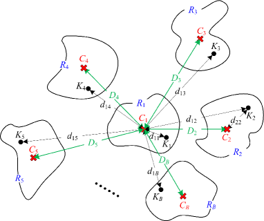
Fig. 1: A schematic model of the considered SCN.

The distance (in km) from the BS of $C_{b}$ to the BS of $C_{1}$, $b\in\left\{1,\ldots,B\right\}$, and the distance from UE $K_{b}$ to the BS of $C_{m}$, $b,m\in\left\{1,\ldots,B\right\}$, are denoted by $D_{b}$ and $d_{bm}$, respectively. In this paper, we consider a deterministic deployment of BSs, and thus the set $\left\{D_{b}\right\}$ is assumed to be known. However, UE $K_{b}$ is assumed to be randomly distributed in $R_{b}$ with a distribution function $f_{Z_{b}}\left(z\right),z\in R_{b}$. Hence, $d_{bm}$ is a random variable (RV), whose distribution cannot be readily expressed in an analytical form due to the arbitrary shape and size of $R_{b}$, and the arbitrary form of $f_{Z_{b}}\left(z\right)$. Unlike the existing works, e.g., [2-8], that only treat uniform UE distributions, in this work we investigate a general probability density function (PDF) of UE distribution denoted by $f_{Z_{b}}\left(z\right)$, which satisfies $0<f_{Z_{b}}\left(z\right)<+\infty,z\in R_{b},$ and its integral over $R_{b}$ equals to one, i.e., $\int_{R_{b}}f_{Z_{b}}\left(z\right)dz=1$.

In the following, we present the modeling of path loss, shadow fading, UL transmission power, and multi-path fading, respectively.

Based on the definition of $d_{bm}$, the path loss (in dB) from UE $K_{b}$ to the BS of $C_{m}$ is modeled as

$$L_{bm}={A}+{\alpha}{\log_{10}}{d_{bm}},$$ (1)

where $A$ is the path loss at the reference distance of $d_{bm}=1$ and $\alpha$ is the path loss exponent. In practice, $A$ and $\alpha$ are constants obtainable from field tests [14]. Note that $L_{bm}$ is a RV due to the randomness of $d_{bm}$.

The shadow fading (in dB) from UE $K_{b}$ to the BS of $C_{m}$ is denoted by $S_{bm}$, and it is usually modeled as a zero-mean Gaussian RV because the linear-scale value of $S_{bm}$ is commonly assumed to follow a lognormal distribution [14]. Hence, in this paper, we model $S_{bm}$ as an independently and identically distributed (i.i.d.) zero-mean Gaussian RV with variance $\sigma_{\textrm{Shad}}^{2}$, denoted by $S_{bm}\sim\mathcal{N}\left(0,\sigma_{\textrm{Shad}}^{2}\right)$ .

The UL transmission power (in dBm) of UE $K_{b}$ is denoted by $P_{b}$. In practice, $P_{b}$ is usually subject to a semi-static power control (PC) mechanism, e.g., the fractional pathloss compensation (FPC) scheme [14]. Based on this FPC scheme, $P_{b}$ in dBm is modeled as

$$P_{b}={P_{0}}+\eta\left({L_{bb}+S_{bb}}\right),$$ (2)

where $P_{0}$ is the target received power at the BS in dBm on the considered frequency RB, $\eta\in\left(0,1\right]$ is the FPC factor, $L_{bb}$ has been defined in (1), and $S_{bb}\sim\mathcal{N}\left(0,\sigma_{\textrm{Shad}}^{2}\right)$ has been discussed above.

The multi-path fading channel from UE $K_{b}$ to the BS of $C_{m}$ is denoted by ${\bf{h}}_{bm}\in\mathbb{C}$, where we assume that each UE and each BS are equipped with one omni-directional antenna. In this paper, we consider a general type of multi-path fading by assuming that the effective channel gain (in dB) associated with ${\bf{h}}_{bm}$ is defined as $10\log_{10}\left|{\bf{h}}_{bm}\right|^{2}$ and denoted by $H_{bm}$, which follows an i.i.d. distribution with the PDF of $f_{H}\left(h\right)$. For example, $\left|{\bf{h}}_{bm}\right|^{2}$ can be respectively characterized by an exponential distribution or a non-central chi-squared distribution in case of Rayleigh fading or Rician fading [15].

III Analysis of the UL Interference Distribution

Based on the definition of RVs discussed in Section II, the UL received interference power (in dBm) from UE $K_{b}$ to the BS of $C_{1}$ can be written as

$$I_{b} \overset{(a)}{=} P_{b}-L_{b1}-S_{b1}+H_{b1}$$ (3)

$$= P_{0}+\left(\eta L_{bb}-L_{b1}\right)+\left(\eta S_{bb}-S_{b1}\right)+H_{b1}$$

$$\overset{\triangle}{=} \left(P_{0}+L+S\right)+H_{b1},$$

$$\overset{\triangle}{=} I_{b}^{\left(1\right)}+H_{b1},$$

where (2) is plugged into the step (a) of (3), and $L$ and $S$ are defined as $L\overset{\triangle}{=}\left(\eta L_{bb}-L_{b1}\right)$ and $S\overset{\triangle}{=}\left(\eta S_{bb}-S_{b1}\right)$, respectively. Apparently, $L$ and $S$ are independent RVs. Besides, the first part of $I_{b}$ is further defined as $I_{b}^{\left(1\right)}\overset{\triangle}{=}\left(P_{0}+L+S\right)$. Since $S_{bb}$ and $S_{b1}$ $\left(b\in\left\{2,\ldots,B\right\}\right)$ are i.i.d. zero-mean Gaussian RVs, it is easy to show that $S$ is also a Gaussian RV, whose mean and variance are

$$\begin{cases}\mu_{S}=0&\\ \sigma_{S}^{2}=\left(1+\eta^{2}\right)\sigma_{\textrm{Shad}}^{2}&\end{cases}.$$ (4)

From the definition of $I_{b}$ in (3), the aggregate interference power (in mW) from all interfering UEs to the BS of $C_{1}$ can be written as

$$I^{\textrm{mW}}=\sum\limits_{b=2}^{B}{10^{\frac{1}{10}I_{b}}}.$$ (5)

In the following subsections, we will analyze the distribution of $I^{\textrm{mW}}$ in three steps:

• First, we investigate the distribution of $I_{b}^{\left(1\right)}$ shown in (3) and approximate such distribution by a Gaussian distribution. The upper-bound of the approximation error measured by the Kolmogorov–Smirnov (KS) [13] distance is derived in closed-form expressions.

• Second, we analyze the sum of RVs $\left(I_{b}^{\left(1\right)}+H_{b1}\right)$ shown in (3) and further approximate the distribution of $I_{b}$ by another Gaussian distribution. The upper-bound of the approximation error measured by the KS distance [13] is derived in closed-form expressions.

• Third, we show that the distribution of $I^{\textrm{mW}}$ can be well approximated by a power lognormal distribution, i.e., with the CDF being a power function of the CDF of a lognormal distribution.

III-A The Distribution of $I_{b}^{\left(1\right)}$ in (3)

Considering the complicated mathematical form of $L$ in (3), we can find that the PDF of $L$ is generally not tractable because $L$ is a RV with respect to $d_{bb}$ and $d_{b1}$, which jointly depend on the arbitrary shape/size of $R_{b}$ and the arbitrary form of $f_{Z_{b}}\left(z\right)$. Specifically, for any point $z\in R_{b}$, $d_{bb}$ and $d_{b1}$ are geometric functions of $z$, and the probability density of $z$ is $f_{Z_{b}}\left(z\right)$. Despite the intractable nature of $L$, we will show that $I_{b}^{\left(1\right)}$ can still be approximated by a Gaussian RV with bounded approximation errors. In more detail, we investigate an upper bound on the error in approximating the sum of an arbitrary RV and a Gaussian RV, i.e., $\left(L+S\right)$, by another Gaussian RV. To that end, we denote by $\mu_{L}$ and $\sigma_{L}^{2}$ the mean and variance of $L$ respectively. Moreover, we define two zero-mean RVs as $\tilde{L}=L-\mu_{L}$ and $\tilde{S}=S-\mu_{S}$, respectively. As a result, $I_{b}^{\left(1\right)}$ in (3) can be re-written as

$$I_{b}^{\left(1\right)}=\left(\tilde{L}+\tilde{S}\right)+\left(P_{0}+\mu_{L}+\mu_{S}\right).$$ (6)

Next, we approximate $\left(\tilde{L}+\tilde{S}\right)$ by a Gaussian RV. And it follows that $I_{b}^{\left(1\right)}$ can also be approximated by the same Gaussian RV with an offset $\left(P_{0}+\mu_{L}+\mu_{S}\right)$.

III-A1 The Distribution of $\left(\tilde{L}+\tilde{S}\right)$ in (6)

 

For the convenience of mathematical expression, the mean, the variance, the 3rd moment and the 4th moment of $\tilde{L}$ are denoted by $\mu_{\tilde{L}}=0$, $\sigma_{\tilde{L}}^{2}=\sigma_{L}^{2}$, $\rho_{\tilde{L}}^{\left(3\right)}$ and $\rho_{\tilde{L}}^{\left(4\right)}$, respectively. Besides, considering (4), the mean and the variance of $\tilde{S}$ are denoted by $\mu_{\tilde{S}}=0$, $\sigma_{\tilde{S}}^{2}=\sigma_{S}^{2}$, respectively. Moreover, we define $\tilde{G}\overset{\triangle}{=}\tilde{L}+\tilde{S}$ and denote the PDF of $\tilde{L}$ by $f_{\tilde{L}}\left(l\right)$.

In order to quantify the approximation error between the distribution $\tilde{G}$ and its approximate Gaussian distribution, we invoke the following definition on the Kolmogorov–Smirnov (KS) distance between two CDFs [13].

Definition 1.

Suppose that the CDFs of RVs $X$ and $\hat{X}$ are $F_{X}\left(x\right)$ and $F_{\hat{X}}\left(x\right)$, respectively. Then the Kolmogorov–Smirnov (KS) distance between $F_{X}\left(x\right)$ and $F_{\hat{X}}\left(x\right)$ is defined as

$$KS\left(X,Y\right)=\underset{x\in\mathbb{R}}{\sup}\left|F_{X}\left(x\right)-F_{\hat{X}}\left(x\right)\right|.$$ (7)

The KS distance is a widely used metric to measure the difference between two CDFs. Based on Definition 1, we present Theorem 2 in the following to bound the KS distance between the CDF of $\tilde{G}$ and that of the corresponding approximate zero-mean Gaussian RV with a variance of $\left(\sigma_{L}^{2}+\sigma_{S}^{2}\right)$.

Theorem 2.

Considering the zero-mean RV $\tilde{G}=\tilde{L}+\tilde{S}$ given by (6), the KS distance between the CDF of $\tilde{G}$ and that of the corresponding approximate zero-mean Gaussian RV with a variance of $\left(\sigma_{L}^{2}+\sigma_{S}^{2}\right)$ is bounded by

$$\underset{g\in\mathbb{R}}{\sup}\left|F_{\tilde{G}}\left(g\right)-\Phi\left(\frac{g}{\sqrt{\sigma_{L}^{2}+\sigma_{S}^{2}}}\right)\right|\leq\max\left\{\varepsilon_{1}+\varepsilon_{2},\>\varepsilon_{3}\right\},$$ (8)

where $F_{\tilde{G}}\left(g\right)$ and $\Phi\left(\cdot\right)$ are respectively the CDF of $\tilde{G}$ and the CDF of the standard normal distribution, and $\max\left\{x,y\right\}$ extracts the larger value between $x$ and $y$.

Furthermore, $\varepsilon_{1}$ in (8) is expressed as

$$\varepsilon_{1}=\frac{1}{2}\delta_{1}\left(\omega,p\right)\frac{1}{k_{2}^{2}}+\frac{1}{2}\delta_{0}\left(\omega,p,\frac{\left(k_{1}+k_{2}\right)\sqrt{\sigma_{L}^{2}+\sigma_{S}^{2}}}{\sqrt{2}\sigma_{S}}\right)+\frac{1}{2}\delta_{0}\left(\frac{\omega\sqrt{\sigma_{L}^{2}+\sigma_{S}^{2}}}{\sigma_{S}},p,\frac{k_{1}}{\sqrt{2}}\right),$$ (9)

where $\omega$, $p$, $k_{1}$ and $k_{2}$ are positive scalars. Besides, $f_{\tilde{L}}\left(l\right)$ is the PDF of $\tilde{L}$, and $\delta_{0}\left(\omega,p,k\right)$ and $\delta_{1}\left(\omega,p,k\right)$ are given by

$$\begin{cases}\delta_{0}\left(\omega,p,k\right)=\frac{2}{\sqrt{\pi}\omega}\textrm{erfc}\left(\left(2p+1\right)\omega\right)+\textrm{erfc}\left(\frac{\pi}{2\omega}-k\right)&\\ \delta_{1}\left(\omega,p\right)=\frac{2}{\sqrt{\pi}\omega}\textrm{erfc}\left(\left(2p+1\right)\omega\right)+2&\end{cases},$$ (10)

where $\textrm{erfc}\left(\cdot\right)$ is the complementary error function [15].

Moreover, $\varepsilon_{2}$ in (8) is given by

$$\varepsilon_{2}=\frac{2}{\pi}\sum_{n=1,n\textrm{ odd}}^{2p-1}\left|\upsilon_{n}-\hat{\upsilon}_{n}\right|,$$ (11)

where $\upsilon_{n}=\frac{1}{n}\exp\left(-\frac{n^{2}\omega^{2}}{2}\right)\varphi_{\tilde{L}}\left(-\frac{n\omega}{\sigma_{S}}\right)$, $\hat{\upsilon}_{n}=\frac{1}{n}\exp\left(-\frac{n^{2}\omega^{2}}{2}\left(\frac{\sigma_{L}^{2}+\sigma_{S}^{2}}{\sigma_{S}^{2}}\right)\right)$, and $\varphi_{\tilde{L}}\left(t\right)$ is the characteristic function [16] of $f_{\tilde{L}}\left(l\right)$.

Finall, $\varepsilon_{3}$ in (8) is expressed as

$$\varepsilon_{3}=\frac{1}{k_{1}^{2}}+\frac{1}{2}\textrm{erfc}\left(k_{1}\right).$$ (12)

Proof:

See Appendix A. ∎

Theorem 2 is useful to quantify the maximum error of approximating $\tilde{G}$ by a Gaussian RV. From the proof in Appendix A, it can be seen that

• $\varepsilon_{1}$ in (8) is caused by the residual errors from the $p$-truncated Fourier series expansion of $\textrm{erfc}\left(\cdot\right)$, where $p$ is the number of the truncated terms.

• $\varepsilon_{2}$ in (8) is the major contributor to the derived upper-bound of the KS distance in Theorem 2.

• $\varepsilon_{3}$ in (8) measures the asymptotic difference between $F_{\tilde{G}}\left(g\right)$ and $\Phi\left(\frac{g}{\sqrt{\sigma_{L}^{2}+\sigma_{S}^{2}}}\right)$ for $\left|g\right|\geq k_{1}\sqrt{\sigma_{L}^{2}+\sigma_{S}^{2}}$, where $k_{1}$ takes a large value to show the asymptotic behavior of the interested CDFs.

To obtain some insights on the typical values of $\varepsilon_{1}$, $\varepsilon_{2}$ and $\varepsilon_{3}$, we should first discuss the appropriate choices of the values of $\omega$, $p$, $k_{1}$ and $k_{2}$. To that end, we have the following remarks.

Remark 1: $\omega$ is the fundamental frequency of the Fourier series expansion of $\textrm{erfc}\left(\cdot\right)$, and thus it should satisfy the condition that $\frac{1}{\omega}$ is much larger than the spread of $x$ in $\textrm{erfc}\left(x\right)$ [15], which can be estimated to be in the range of $\left[-5,5\right]$ because $\left|\textrm{erfc}\left(-\infty\right)-\textrm{erfc}\left(-5\right)\right|=1.54\times 10^{-12}\approx 0$ and $\left|\textrm{erfc}\left(+\infty\right)-\textrm{erfc}\left(5\right)\right|=1.54\times 10^{-12}\approx 0$. Therefore, $\frac{1}{\omega}$ should be much larger than 10 due to the range of $\left[-5,5\right]$. We propose that a typical value of $\frac{1}{\omega}$ could be 1000, i.e., $\omega=0.001$.

Remark 2: $p$ is the number of the truncated terms in the $p$-truncated Fourier series expansion of $\textrm{erfc}\left(\cdot\right)$, and thus it should be sufficiently large to make the residual error caused by the truncation of the Fourier series expansion very small. The part of the residual error that is related to $p$, is expressed as $\tilde{\delta}\left(\omega,p\right)=\frac{2}{\sqrt{\pi}\omega}\textrm{erfc}\left(\left(2p+1\right)\omega\right)$ in (10). From this expression, we can see that $p$ should be larger than $\frac{2}{\omega}$ to make $\tilde{\delta}\left(\omega,p\right)$ sufficiently small, because $\textrm{erfc}\left(\left(2\times\frac{2}{\omega}+1\right)\omega\right)=1.4\times 10^{-8}$ when $\omega=0.001$. We propose that a typical value of $p$ could be $\frac{4}{\omega}$, which equals to 4000 when $\omega=0.001$. The corresponding $\tilde{\delta}\left(\omega,p\right)$ will then drop to a very small value of $1.1\times 10^{-27}$.

Remark 3: Since $k_{1}$ is related to the asymptotic behavior of $F_{\tilde{G}}\left(g\right)$ and $\Phi\left(\frac{g}{\sqrt{\sigma_{L}^{2}+\sigma_{S}^{2}}}\right)$ when $\left|g\right|\geq k_{1}\sqrt{\sigma_{L}^{2}+\sigma_{S}^{2}}$, and thus $k_{1}$ should be sufficiently large to make $\varepsilon_{3}$ a small value. We propose that the typical value of $k_{1}$ should be at least 100 to achieve an $\varepsilon_{3}$ as small as $1.0\times 10^{-4}$, which corresponds to a small error of $\pm 0.01$ percentile. As will be shown in Section IV, $k_{1}$ is set to 500, and we have $\varepsilon_{3}=4\times 10^{-6}$, which is confirmed to be always smaller than $\varepsilon_{2}$ in our numerical results.

Remark 4: As discussed in Appendix A, the introduction of $k_{2}$ is to facilitate the bounding of the integral over $l$ from $-\infty$ to $+\infty$. From (9), the first term of (9), i.e., $\frac{1}{2}\delta_{1}\left(\omega,p\right)\frac{1}{k_{2}^{2}}$, dominates $\varepsilon_{1}$ because $\delta_{0}\left(\omega,p,k\right)$ is a very small value with appropriate choices of $\omega$, $p$, $k_{1}$ and $k_{2}$. For example, as discussed above, we choose $\omega=0.001$, $p=4000$, $k_{1}=k_{2}=500$, and $\sigma_{L}=\sigma_{S}$, then the first term of (9) becomes $4\times 10^{-6}$, while the sum of the rest terms is merely $6.3\times 10^{-27}$. Since a larger $k_{2}$ directly leads to a smaller $\varepsilon_{1}$, we propose that the typical value of $k_{2}$ should be at least 100 to achieve an $\varepsilon_{1}$ as small as $1.0\times 10^{-4}$, which corresponds to a small error of $\pm 0.01$ percentile. As will be shown in Section IV, $k_{2}$ is set to 500, and we have $\varepsilon_{1}=4\times 10^{-6}$, which is confirmed to be always smaller than $\varepsilon_{2}$ in our numerical results.

Considering the expressions of $\varepsilon_{1}$ and $\varepsilon_{3}$ shown in (9) and (12), respectively, we investigate a special case of $k_{1}=k_{2}$ and it is straightforward to get $\varepsilon_{1}>\varepsilon_{3}$. Hence, we propose the following corollary to simplify Theorem 2.

Corollary 3.

When $k_{1}=k_{2}$, the KS distance between the CDF of $\tilde{G}$ and that of the corresponding approximate zero-mean Gaussian RV with a variance of $\left(\sigma_{L}^{2}+\sigma_{S}^{2}\right)$ is bounded by

$$\underset{g\in\mathbb{R}}{\sup}\left|F_{\tilde{G}}\left(g\right)-\Phi\left(\frac{g}{\sqrt{\sigma_{L}^{2}+\sigma_{S}^{2}}}\right)\right|\leq\varepsilon_{1}+\varepsilon_{2}.$$ (13)

Note that compared with (8), $\varepsilon_{3}$ does not exist in the right-hand side of (13), which largely simplifies our analysis and discussion. Therefore, in the sequel we will only consider (13) to quantify the maximum error of approximating $\tilde{G}$ by a Gaussian RV.

With the discussed typical values of $\omega$, $p$, $k_{1}$ and $k_{2}$, we can see that $\varepsilon_{1}$ in (13) can be controlled to be as small as $4\times 10^{-6}$, which leaves $\varepsilon_{2}$ as the major contributor to the derived upper-bound of the KS distance. We will briefly discuss the calculation of $\varepsilon_{2}$ in the next subsection. Note that further optimization of $k_{1}$ and $k_{2}$ to reduce $\varepsilon_{3}$ and $\varepsilon_{1}$ even below $4\times 10^{-6}$ is possible. However, such optimization has a marginal impact on the derived upper bound of the approximation error because $\varepsilon_{2}$ is independent of $k_{1}$ and $k_{2}$.

With Theorem 2 and Corollary 3 characterizing the upper bound of the approximation error, we propose to approximate $I_{b}^{\left(1\right)}$ in (6) by a Gaussian RV $G_{b}$, whose mean and variance can be computed by

$$\begin{cases}\mu_{G_{b}}=P_{0}+\mu_{L}+\mu_{S}&\\ \sigma_{G_{b}}^{2}=\sigma_{L}^{2}+\sigma_{S}^{2}&\end{cases}.$$ (14)

III-A2 The Calculation of $\varepsilon_{2}$ in (11)

 

For each small cell $C_{b}$, considering the definition of $L$ and $\tilde{L}$ respectively presented in (3) and (6), we can evaluate $\varphi_{\tilde{L}}\left(-\frac{n\omega}{\sigma_{S}}\right)$ for each small cell $C_{b}$ as

$$\varphi_{\tilde{L}}\left(-\frac{n\omega}{\sigma_{S}}\right) = \int_{-\infty}^{+\infty}\exp\left(-\textrm{j}\frac{n\omega l}{\sigma_{S}}\right)f_{\tilde{L}}\left(l\right)dl$$ (15)

$$= \int_{R_{b}}\exp\left(-\textrm{j}n\omega\frac{L\left(z\right)-\mu_{L}}{\sigma_{S}}\right)f_{Z_{b}}\left(z\right)dz$$

$$\overset{\left(a\right)}{=} \int_{R_{b}}\exp\left(-\textrm{j}n\omega\frac{\eta L_{bb}\left(z\right)-L_{b1}\left(z\right)-\mu_{L}}{\sigma_{S}}\right)f_{Z_{b}}\left(z\right)dz,$$

where (1) should be inserted into the step (a) of (15) and $\mu_{L}$ is the mean of $L$.

With the result of $\varphi_{\tilde{L}}\left(-\frac{n\omega}{\sigma_{S}}\right)$, we can then compute $\varepsilon_{2}$ according to its definition in (11).

III-B The Distribution of $I_{b}$ in (3)

Having approximated $I_{b}^{\left(1\right)}$ by a Gaussian RV $G_{b}$, we can approximate (3) as

$$I_{b}\approx G_{b}+H_{b1}.$$ (16)

It is interesting to note that, similar to $I_{b}^{\left(1\right)}$ in (3), the approximate expression of $I_{b}$ in (16) also contains a Gaussian RV $G_{b}$ and an arbitrary RV $H_{b1}$ with the PDF of $f_{H}\left(h\right)$.

Based on the above observation, we propose to reuse Theorem 2 and Corollary 3 to quantify the error in approximating $I_{b}$ in (16) by an another Gaussian RV. To that end, similar to (6), we define two zero-mean RVs as $\tilde{G}_{b}=G_{b}-\mu_{G_{b}}$ and $\tilde{H}_{b1}=H_{b1}-\mu_{H_{b1}}$, where $\mu_{G_{b}}$ and $\mu_{H_{b1}}$ are the means of $G_{b}$ and $H_{b1}$, respectively. Besides, the variance of $G_{b}$ and $H_{b1}$ are denoted by $\sigma_{G_{b}}^{2}$ and $\sigma_{H_{b1}}^{2}$, respectively. As a result, we can re-formulate (16) as

$$I_{b}\approx\left(\tilde{G}_{b}+\tilde{H}_{b1}\right)+\left(\mu_{G_{b}}+\mu_{H_{b1}}\right).$$ (17)

Next, we approximate $\left(\tilde{G}_{b}+\tilde{H}_{b1}\right)$ by a Gaussian RV. And it follows that $I_{b}$ can also be approximated by the same Gaussian RV with an offset $\left(\mu_{G_{b}}+\mu_{H_{b1}}\right)$.

III-B1 The Distribution of $\left(\tilde{G}_{b}+\tilde{H}_{b1}\right)$ in (17)

 

We propose to approximate $\left(\tilde{G}_{b}+\tilde{H}_{b1}\right)$ as a zero-mean Gaussian RV with a variance of $\sigma_{G_{b}}^{2}+\sigma_{H_{b1}}^{2}$, then from Corollary 3, the error measured by the KS distance between the actual CDF and the approximate CDF can be upper-bounded by $\varepsilon^{\prime}_{1}+\varepsilon^{\prime}_{2}$, where $\varepsilon^{\prime}_{1}$ and $\varepsilon^{\prime}_{2}$ are respectively computed using (9) and (11) with the following RV changes,

$$\begin{cases}\varepsilon^{\prime}_{1}=\left[\varepsilon_{1}\left|S\rightarrow G_{b},\tilde{S}\rightarrow\tilde{G}_{b},L\rightarrow H_{b1},\tilde{L}\rightarrow\tilde{H}_{b1}\right.\right]&\\ \varepsilon^{\prime}_{2}=\left[\varepsilon_{2}\left|S\rightarrow G_{b},\tilde{S}\rightarrow\tilde{G}_{b},L\rightarrow H_{b1},\tilde{L}\rightarrow\tilde{H}_{b1}\right.\right]&\end{cases},$$ (18)

where $X\rightarrow Y$ denotes the RV change of replacing $X$ with $Y$.

III-B2 The approximate PDF and CDF of $I_{b}$

 

With the approximation of $\left(\tilde{G}_{b}+\tilde{H}_{b1}\right)$ as a zero-mean Gaussian RV, we propose to approximate $I_{b}$ in (17) as another Gaussian RV $Q_{b}$, whose mean and variance are

$$\begin{cases}\mu_{Q_{b}}=\mu_{G_{b}}+\mu_{H_{b1}}&\\ \sigma_{Q_{b}}^{2}=\sigma_{G_{b}}^{2}+\sigma_{H_{b1}}^{2}&\end{cases}.$$ (19)

According to Theorem 2 and Corollary 3, and from (9), (11) and (18), the total error of approximating $I_{b}$ as $Q_{b}$, measured by the KS distance between the CDF of $I_{b}$ and that of $Q_{b}$, can be upper-bounded by $\varepsilon$ as

$$\varepsilon=\left(\varepsilon_{1}+\varepsilon_{2}\right)+\left(\varepsilon^{\prime}_{1}+\varepsilon^{\prime}_{2}\right),$$ (20)

where $\left(\varepsilon_{1}+\varepsilon_{2}\right)$ is the upper bound on the error associated with the approximation of $I_{b}^{\left(1\right)}$ in (6) as a Gaussian RV $G_{b}$, and $\left(\varepsilon^{\prime}_{1}+\varepsilon^{\prime}_{2}\right)$ is the upper bound on the error associated with the approximation of $G_{b}+H_{b1}$ in (16) as a Gaussian RV $Q_{b}$.

III-C The Distribution of $I^{\textrm{mW}}$ in (5)

The study on the approximate distribution of the sum of multiple independent lognormal RVs has been going on for more than five decades [17]-[21]. According to [17]-[18], the sum of multiple independent lognormal RVs can be well approximated by another lognormal RV. However, some recent studies [19]-[21] concluded that the sum of multiple independent lognormal RVs is better approximated by a power lognormal RV, i.e., with the CDF being a power function of $\Phi\left(\cdot\right)$. In this paper, we adopt the power lognormal approximation for $I^{\textrm{mW}}$, which will be explained in the following.

In our case, since each $I_{b},b\in\left\{2,\dots,B\right\}$ is approximated by the Gaussian RV $Q_{b}$, the sum of $10^{\frac{1}{{10}}Q_{b}}$ can be well approximated by a power lognormal RV [19]-[21] expressed as $\hat{I}^{\textrm{mW}}=10^{\frac{1}{{10}}Q}$, where the PDF and CDF of $Q$ can be respectively written as [19]

$$\begin{cases}\textrm{PDF of }Q:\>{f_{Q}}\left(q\right)=\lambda\Phi^{\lambda-1}\left(\frac{q-{\mu_{Q}}}{\sigma_{Q}}\right)\frac{1}{\sqrt{2\pi\sigma_{Q}^{2}}}\exp\left\{{-\frac{{\left({q-{\mu_{Q}}}\right)^{2}}}{{2\sigma_{Q}^{2}}}}\right\}&\\ \textrm{CDF of }Q:\>{F_{Q}}\left(q\right)=\Phi^{\lambda}\left(\frac{q-{\mu_{Q}}}{\sigma_{Q}}\right)&\end{cases},$$ (21)

where the parameters $\lambda$, $\mu_{Q}$ and $\sigma_{Q}$ are obtained from $\left\{\mu_{Q_{b}}\right\}$ and $\left\{\sigma_{Q_{b}}^{2}\right\}$. The method to accomplish such task has been well addressed in [19]-[21]. In Appendix B, we provide an example to obtain $\lambda$, $\mu_{Q}$ and $\sigma_{Q}$ based on [17], [20] and [21].

As a result of (21), the PDF and CDF of $\hat{I}^{\textrm{mW}}$ can be respectively written as

$$\begin{cases}\textrm{PDF of }\hat{I}^{\textrm{mW}}:\>{f_{\hat{I}^{\textrm{mW}}}}\left(v\right)=\lambda\Phi^{\lambda-1}\left(\frac{\zeta\ln v-{\mu_{Q}}}{\sigma_{Q}}\right)\frac{\zeta}{v\sqrt{2\pi\sigma_{Q}^{2}}}\exp\left\{{-\frac{{\left({\zeta\ln v-{\mu_{Q}}}\right)^{2}}}{{2\sigma_{Q}^{2}}}}\right\}&\\ \textrm{CDF of }\hat{I}^{\textrm{mW}}:\>{F_{\hat{I}^{\textrm{mW}}}}\left(v\right)=\Phi^{\lambda}\left(\frac{\zeta\ln v-{\mu_{Q}}}{\sigma_{Q}}\right)&\end{cases},$$ (22)

where $\zeta=\frac{10}{\ln 10}$ is a scalar caused by the variable change from $10\log_{10}v$ to $\ln v$.

Finally, we propose that the distribution of $I^{\textrm{mW}}$ can be approximated by that of $\hat{I}^{\textrm{mW}}$ shown in (22). Note that in this step of approximation, the approximation error is dependent on the adopted approximate distribution of the sum of multiple independent lognormal RVs. We will study such approximation error in our future work. Note that some recent studies [19]-[21] have shown that the error associated with the power lognormal approximation is reasonably small and good enough for practical use.

III-D Summary of the Proposed Analysis of the UL Interference Distribution

To sum up, in the following, we highlight the main steps in our proposed microscopic analysis of the UL interference distribution. First, for each $b\in\left\{2,\ldots,B\right\}$, we use (9) and (11) to check $\left(\varepsilon_{1}+\varepsilon_{2}\right)$ associated with the approximation of $I_{b}^{\left(1\right)}$ in (6) as a Gaussian RV $G_{b}$. Second, for each $b\in\left\{2,\ldots,B\right\}$, we use (18) to check $\left(\varepsilon^{\prime}_{1}+\varepsilon^{\prime}_{2}\right)$ associated with the approximation of $G_{b}+H_{b1}$ in (16) as a Gaussian RV $Q_{b}$. The upper bound of the total approximation error of the above two steps is further obtained from (20), without any requirement on (i) the shape and/or size of cell coverage areas, (ii) the uniformity of UE distribution, and (iii) the type of multi-path fading. Finally, we approximate $I^{\textrm{mW}}$ in (5) by a power lognormal RV $\hat{I}^{\textrm{mW}}=10^{\frac{1}{{10}}Q}$, where the PDF and the CDF of $Q$ is expressed as (21) with the parameters $\lambda$, $\mu_{Q}$ and $\sigma_{Q}^{2}$ obtained from, e.g., Appendix B.

IV Simulation and Discussion

In order to validate the approximation from the proposed microscopic analysis of the UL interference, we conduct simulations considering two types of scenarios, i.e., one with a single interfering cell and the other with multiple interfering cells. As discussed in Remarks 1~4 in Subsection III-A1, the parameters for evaluating Theorem 2 and Corollary 3 are set to: $\omega=0.001$, $p=4000$, $k_{1}=k_{2}=500$. According to the 3GPP standards [14], the system parameters are set to: $A=103.8$, $\alpha=20.9$, $P_{0}=-76$ dBm, $\eta=0.8$, and $\sigma_{S}=10$ dB. Besides, the minimum BS-to-UE distance is assumed to be 0.005 km [14].

IV-A The Scenario with a Single Interfering Cell

In this scenario, the number of BSs $B$ is set to 2, and UEs in small cell $C_{2}$ are assumed to be uniformly distributed and non-uniformly distributed in the coverage area $R_{2}$, respectively.

IV-A1 Uniformly Distributed UEs

 

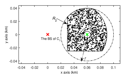
Fig. 2: Illustration of the coverage area $R_{2}$ ($r=0.04\,\textrm{km}$, uniformly distributed UEs).

In this case, we consider uniformly distributed UEs, as shown in Fig. 2. The x-markers indicate BS locations where the BS location of $C_{1}$ has been explicitly pointed out. The dash-dot line indicates a reference disk to illustrate the reference size of small cell $C_{2}$. The radius of such a reference circle is denoted by $r$, and the distance between the BS of $C_{1}$ and the BS of $C_{2}$, i.e., $D_{2}$, is assumed to be $1.5r$. Note that $1.5r$ is just an example of $D_{2}$ and the specific value of $D_{2}$ has no impact on the procedure of our analysis. In our simulations, the values of $r$ (in km) are set to 0.01, 0.02 and 0.04, respectively [1]. In this scenario, the interfering UE $K_{2}$ is uniformly distributed in an irregularly shaped coverage area $R_{2}$, as shown by the area outlined by the solid line in Fig. 2. The shape of $R_{2}$ is the intersection of a square, a circle and an ellipse, which has a very complicated generation function. Examples of the possible positions of $K_{2}$ within $R_{2}$ are shown as dots in Fig. 2.

Despite the complicated shape of $R_{2}$, our proposed microscopic analysis of the UL interference distribution still can be applied. Specifically, from Corollary 3, (9), (11), and (18), we can examine the validity of approximating $I_{2}$ as a Gaussian RV by checking the corresponding $\varepsilon$ given by (20). The results of $\varepsilon$ are tabulated for various values of $r$ with the assumption of Rayleigh fading in Table I. Moreover, $\varepsilon$ is broken into $\left(\varepsilon_{1}+\varepsilon_{2}\right)$ and $\left(\varepsilon^{\prime}_{1}+\varepsilon^{\prime}_{2}\right)$, with the marginal contribution of $\varepsilon_{1}$ and $\varepsilon^{\prime}_{1}$ shown in Table I as well. From this table, we can observe that $\varepsilon_{2}$ and $\varepsilon^{\prime}_{2}$ are about $100$ times larger than $\varepsilon_{1}$ and $\varepsilon^{\prime}_{1}$, indicating the dominance of $\varepsilon_{2}$ and $\varepsilon^{\prime}_{2}$ in the result of $\varepsilon$. For all the investigated values of $r$, the values of $\varepsilon$ are below 0.01. Consequently, the approximation of $I_{2}$ as a Gaussian RV should be tight. Note that $r=0.01$ and $r=0.02$ correspond to the typical network configurations for future dense and ultra-dense SCNs [1], which shows that our proposed microscopic analysis of the UL interference distribution can be readily used to study future dense and ultra-dense SCNs. Also note that the upper bound $\varepsilon$ is much tighter than that presented in our previous work [10]. Specifically, when $r=0.04$, the upper bound on the approximation error in [10] is around $1.84\times 10^{-2}$, while in Table I $\varepsilon$ is only $4.6\times 10^{-3}$, which is a significant improvement compared with our previous result in [10].

Table I: Approximation errors of the proposed analysis
($B=2$, uniformly distributed UEs, Rayleigh fading).

$r$	$\varepsilon$	$\varepsilon_{1}+\varepsilon_{2}$	$\varepsilon_{1}$	$\varepsilon^{\prime}_{1}+\varepsilon^{\prime}_{2}$	$\varepsilon^{\prime}_{1}$	$\mu_{Q_{2}}$	$\sigma_{Q_{2}}^{2}$	Actual error
$0.01$	$4.9\times 10^{-3}$	$3.5\times 10^{-4}$	$4\times 10^{-6}$	$4.6\times 10^{-3}$	$4\times 10^{-6}$	-97.1	205.3	$1.9\times 10^{-3}$
$0.02$	$5.0\times 10^{-3}$	$5.2\times 10^{-4}$	$4\times 10^{-6}$	$4.5\times 10^{-3}$	$4\times 10^{-6}$	-99.7	207.7	$1.9\times 10^{-3}$
$0.04$	$4.6\times 10^{-3}$	$1.1\times 10^{-4}$	$4\times 10^{-6}$	$4.5\times 10^{-3}$	$4\times 10^{-6}$	-101.5	211.4	$1.8\times 10^{-3}$

To further verify the accuracy of the proposed approximation, we plot the simulation results of the CDF of $I_{2}$ and the analytical results of the approximate Gaussian CDF according to (19) for the considered $R_{2}$ in Fig. 3. The numerical results of $\mu_{Q_{2}}$ and $\sigma_{Q_{2}}^{2}$ are also listed in Table I. As can be seen from Fig. 3, the proposed Gaussian approximation of $I_{2}$ is very tight for the considered $R_{2}$ with such an irregular shape. Note that the actual errors between the simulation and the approximation of the CDF of $I_{2}$ are also shown in Table I, the results of which establish the validity of the derived upper bound on the approximation error.

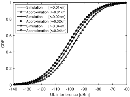
Fig. 3: The simulation and the approximation of the CDF of $I_{2}$ ($B=2$, uniformly distributed UEs, Rayleigh fading).

As discussed above, Table I is obtained with the assumption of Rayleigh fading. In the following, we will check the approximation errors for Rician fading and another case without multi-path fading. According to [15], a ratio between the power in the line-of-sight (LOS) path and the power in the other scattered paths should be defined for Rician fading. Such ratio is denoted by $\Gamma$ in our paper. Note that Rician fading will degrade to Rayleigh fading when $\Gamma=0$. For various values of $r$ under the assumption of Rician fading with $\Gamma=10$, the results of $\varepsilon$ are tabulated in Table II. Comparing Table II with Table I, we can see that the difference lies in the values of $\left(\varepsilon^{\prime}_{1}+\varepsilon^{\prime}_{2}\right)$ because it solely depends on the assumption of multi-path fading as discussed in Subsection III-B1. Note that the errors caused by the consideration of Rician fading is actually smaller than those of Rayleigh fading, because Rician fading incurs less randomness than Rayleigh fading due to the dominant LOS path component in the multi-path fading. Such reduction of randomness can be further observed in an extreme case of $\Gamma=+\infty$, where a deterministic LOS path completely dominates the multi-path fading. The results of $\varepsilon$ for such extreme case with $\Gamma=+\infty$, i.e., no multi-path fading, are exhibited in Table III, where $\varepsilon^{\prime}_{1}$ and $\varepsilon^{\prime}_{2}$ are all zeros because the approximation step addressed in Subsection III-B is skipped, rendering $H_{b1}\equiv 0\,\textrm{dB}$.

For all the investigated values of $r$, the values of $\varepsilon$ are smaller than 0.001 in both Table II and Table III, indicating that the approximation of $I_{2}$ as a Gaussian RV should be even tighter than that observed in Fig. 3. For brevity, we omit these figures. Note that the actual errors between the simulation and the approximation of the CDF of $I_{2}$ are provided in Table II and Table III, the results of which also establish the validity of the derived upper bound $\varepsilon$.

Table II: Approximation errors of the proposed analysis
($B=2$, uniformly distributed UEs, Rician fading with $\Gamma=10$).

$r$	$\varepsilon$	$\varepsilon_{1}+\varepsilon_{2}$	$\varepsilon_{1}$	$\varepsilon^{\prime}_{1}+\varepsilon^{\prime}_{2}$	$\varepsilon^{\prime}_{1}$	$\mu_{Q_{2}}$	$\sigma_{Q_{2}}^{2}$	Actual error
$0.01$	$5.4\times 10^{-4}$	$3.5\times 10^{-4}$	$4\times 10^{-6}$	$1.9\times 10^{-4}$	$4\times 10^{-6}$	-95.0	178.2	$2.0\times 10^{-4}$
$0.02$	$7.0\times 10^{-4}$	$5.2\times 10^{-4}$	$4\times 10^{-6}$	$1.9\times 10^{-4}$	$4\times 10^{-6}$	-97.6	180.8	$4.8\times 10^{-4}$
$0.04$	$3.0\times 10^{-4}$	$1.1\times 10^{-4}$	$4\times 10^{-6}$	$1.9\times 10^{-4}$	$4\times 10^{-6}$	-99.4	184.5	$1.9\times 10^{-4}$

Table III: Approximation errors of the proposed analysis
($B=2$, uniformly distributed UEs, no multi-path fading).

$r$	$\varepsilon$	$\varepsilon_{1}+\varepsilon_{2}$	$\varepsilon_{1}$	$\varepsilon^{\prime}_{1}+\varepsilon^{\prime}_{2}$	$\varepsilon^{\prime}_{1}$	$\mu_{Q_{2}}$	$\sigma_{Q_{2}}^{2}$	Actual error
$0.01$	$3.5\times 10^{-4}$	$3.5\times 10^{-4}$	$4\times 10^{-6}$	0	0	-94.6	174.2	$1.3\times 10^{-4}$
$0.02$	$5.2\times 10^{-4}$	$5.2\times 10^{-4}$	$4\times 10^{-6}$	0	0	-97.2	176.7	$2.4\times 10^{-4}$
$0.04$	$1.1\times 10^{-4}$	$1.1\times 10^{-4}$	$4\times 10^{-6}$	0	0	-99.0	180.5	$0.6\times 10^{-4}$

IV-A2 Non-Uniformly Distributed UEs

 

In this subsection, we further investigate the scenario discussed in Subsection IV-A1. Different from previous assumption, here we consider that the interfering UE $K_{2}$ is no longer uniformly distributed in $R_{2}$. In this subsection, we consider a UE distribution function expressed as $f_{Z_{2}}\left(z\right)=\frac{W}{\rho},z\in R_{2}$, where $\rho$ is the radial coordinate of $z$ in the polar coordinate system, the origin of which is placed at the position of the BS of $C_{2}$. Besides, $W$ is a normalization constant to make $\int_{R_{2}}f_{Z_{2}}\left(z\right)dz=1$. In the considered non-uniform UE distribution, UEs are more likely to locate in the close vicinity of the BS of $C_{2}$, as shown in Fig. 4, where examples of the possible positions of $K_{2}$ within $R_{2}$ are shown as dots. Note that the considered $f_{Z_{2}}\left(z\right)$ is just an example of the non-uniformly distributed UEs in $R_{2}$, which reflects a reasonable network planning that BSs have been deployed at the center spots of UE clusters. Other forms of the UE distribution function will not affect the procedure of our analysis, only the approximation error values may change with the choice of the UE distribution function. Since we have shown in Subsection IV-A1 that Rayleigh fading is the worst case for the proposed analysis, we adopt the assumption of Rayleigh fading in this subsection.

Fig. 4: Illustration of the coverage area $R_{2}$ ($r=0.04\,\textrm{km}$, non-uniformly distributed UEs).

From (20), we can evaluate the quality of approximating $I_{2}$ as a Gaussian RV by checking the corresponding $\varepsilon$. Like Table I, the results of $\varepsilon$ for this network scenario are tabulated for various values of $r$ in Table IV. From Table IV, we can see that the values of $\varepsilon$ are small, i.e., below 0.01, which indicates that the approximation of $I_{2}$ as a Gaussian RV should be tight, as can be confirmed from the actual error values in Table IV.

Table IV: Approximation errors of the proposed analysis ($B=2$, non-uniformly distributed UEs with the distribution function of $f_{Z_{2}}\left(z\right)=\frac{W}{\rho},z\in R_{2}$, Rayleigh fading).

$r$	$\varepsilon$	$\varepsilon_{1}+\varepsilon_{2}$	$\varepsilon_{1}$	$\varepsilon^{\prime}_{1}+\varepsilon^{\prime}_{2}$	$\varepsilon^{\prime}_{1}$	$\mu_{Q_{2}}$	$\sigma_{Q_{2}}^{2}$	Actual error
$0.01$	$4.9\times 10^{-3}$	$4.0\times 10^{-4}$	$4\times 10^{-6}$	$4.5\times 10^{-3}$	$4\times 10^{-6}$	-97.13	205.1	$1.8\times 10^{-3}$
$0.02$	$5.3\times 10^{-3}$	$7.1\times 10^{-4}$	$4\times 10^{-6}$	$4.6\times 10^{-3}$	$4\times 10^{-6}$	-100.6	207.9	$2.2\times 10^{-3}$
$0.04$	$4.9\times 10^{-3}$	$4.0\times 10^{-4}$	$4\times 10^{-6}$	$4.5\times 10^{-3}$	$4\times 10^{-6}$	-103.2	214.4	$1.7\times 10^{-3}$

IV-B The Scenario with Multiple Interfering Cells

In this subsection, we apply the proposed framework to a more complex network with practical deployment of multiple cells and provide the approximation of the UL interference distribution.

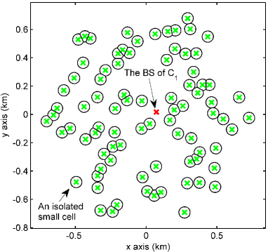
Fig. 5: Illustration of a practical deployment of multiple small cells ($r=0.04\,\textrm{km}$).

Here, we consider a 3GPP-compliant scenario [14], as shown in Fig. 5, where the number of BSs $B$ is set to 84 and all small cell BSs are represented by x-markers. Particularly, the BS of $C_{1}$ has been explicitly pointed out. The reference coverage area for each small cell is a disk with a radius of $r$ [14]. As in previous subsections, the values of $r$ (in km) are set to 0.01, 0.02 and 0.04, respectively. The reference disk-shaped areas can be easily seen in Fig. 5 from any isolated small cell. However, due to the irregular positions of the cells, the actual coverage areas of the considered cells are of irregular shapes. The irregularly shaped coverage areas are outlined by solid lines in Fig. 5.

An important note is that the considered network scenario is different from that adopted in [2,3], where coverage areas are defined as Voronoi cells generated by the Poisson distributed BSs and the entire network area is covered by those Voronoi cells. In practice, small cells are mainly used for capacity boosting in specific populated areas, rather than the provision of an umbrella coverage for all UEs [1]. In this light, the 3GPP standards recommend the hotspot scenario depicted in Fig. 5 for UE distribution in the performance evaluation of practical SCNs and we adopt such network scenario in this subsection. Nevertheless, we should mention that the proposed microscopic analysis of the UL interference distribution can still be applied on a particular Voronoi tessellation. This is because Theorem 2 and Corollary 3 in this paper do not rely on particular shape and/or size of coverage areas.

In this subsection, we consider the same UE distribution function as the one discussed in Subsection IV-A2, i.e., $f_{Z_{b}}\left(z\right)=\frac{W}{\rho},z\in R_{b}$, where $\rho$ is the radial coordinate of $z$ in the polar coordinate system with its origin placed at the position of the BS of $C_{b}$, and $W$ is a normalization constant to make $\int_{R_{b}}f_{Z_{b}}\left(z\right)dz=1$. Besides, we assume Rayleigh fading in this subsection since Rayleigh fading is the worst case for the proposed analysis as addressed in Subsection IV-A1.

In the following, we investigate the considered network with the proposed microscopic analysis of the UL interference distribution. First, for each $R_{b},b\in\left\{2,\ldots,84\right\}$, we invoke (9), (11) and (18) to check the maximum error $\varepsilon$ among $b\in\left\{2,\ldots,84\right\}$ using (20). If the maximum value of $\varepsilon$ is reasonably small, e.g., less than 0.01, then we can approximate $I^{\textrm{mW}}$ in (5) as a power lognormal RV $\hat{I}^{\textrm{mW}}=10^{\frac{1}{{10}}Q}$, where the PDF and the CDF of $Q$ are given by (21) with the parameters $\lambda$, $\mu_{Q}$ and $\sigma_{Q}^{2}$ obtained from, e.g., Appendix B.

The maximum values of the 83 $R_{b}$-specific $\varepsilon$’s for various $r$ values are presented in Table V. From Table V, we can observe that, for all the investigated values of $r$, the maximum values of $\varepsilon$ are below 0.01. Thus, each $I_{b}$ should be well approximated by a Gaussian RV $Q_{b}$. Due to space limitation, we omit the detailed numerical investigation on the Gaussian approximation for each $I_{b}$, which is very similar to the discussion in Subsection IV-A2. After obtaining the approximation for each $I_{b}$, we approximate $I^{\textrm{mW}}$ in (5) as a power lognormal RV $\hat{I}^{\textrm{mW}}=10^{\frac{1}{{10}}Q}$ using (22). The numerical results of $\lambda$, $\mu_{Q}$ and $\sigma_{Q}^{2}$ are provided in Table V for reference.

Table V: Approximation errors of the proposed analysis ($B=84$, non-uniformly distributed UEs with the distribution function of $f_{Z_{b}}\left(z\right)=\frac{W}{\rho},z\in R_{b}$, Rayleigh fading).

$r$	Max $\varepsilon$	Max $\varepsilon_{1}+\varepsilon_{2}$	Max $\varepsilon_{1}$	Max $\varepsilon^{\prime}_{1}+\varepsilon^{\prime}_{2}$	Max $\varepsilon^{\prime}_{1}$	$\lambda$	$\mu_{Q}$	$\sigma_{Q}^{2}$
$0.01$	$5.1\times 10^{-3}$	$2.7\times 10^{-4}$	$4\times 10^{-6}$	$4.8\times 10^{-3}$	$4\times 10^{-6}$	48.9	-99.7	116.2
$0.02$	$5.1\times 10^{-3}$	$4.2\times 10^{-4}$	$4\times 10^{-6}$	$4.7\times 10^{-3}$	$4\times 10^{-6}$	48.0	-101.6	116.5
$0.04$	$5.9\times 10^{-3}$	$1.2\times 10^{-3}$	$4\times 10^{-6}$	$4.7\times 10^{-3}$	$4\times 10^{-6}$	47.5	-103.1	117.2

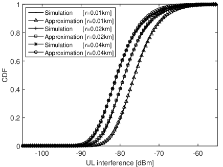
Fig. 6: The simulation and the approximation of the CDF of $I^{\textrm{mW}}$ in dBm ($B=84$, non-uniformly distributed UEs with the distribution function of $f_{Z_{b}}\left(z\right)=\frac{W}{\rho},z\in R_{b}$, Rayleigh fading).

To further verify the accuracy of our analytical results on the UL interference distribution, in Fig. 6 we plot the simulation results of the CDF of $I^{\textrm{mW}}$ in dBm and the approximate analytical results according to (22). As can be seen from Fig. 6, the resulting power lognormal approximation of $I^{\textrm{mW}}$ is tight. However, note that the approximation shown in Fig. 6 is not as perfect as that exhibited in Fig. 3. According to the discussion in Section III, the approximation errors associated with the first and the second steps of approximation are captured in $\varepsilon$, which is very small as can be confirmed from Table V. The noticeable small approximation errors in Fig. 6 are caused by the inaccuracy of approximating the sum of multiple lognormal RVs as a single power lognormal RV. Note that in our previous work [10], we use a lognormal RV to approximate the sum of multiple lognormal RVs, which leads to larger errors compared with the results shown in Fig. 6. Finding an even better distribution to approximate the CDF of the sum of multiple lognormal RVs will be our future work.

IV-C Discussion on the Complexity of the Proposed Microscopic Analysis

The computational complexity of the proposed approach is mainly attributable to the numerical integration required to obtain the values of $\varepsilon$ for each small cell. In contrast, the simulation approach, e.g., [8], [9], as well as in this paper, involves a tremendously high complexity. Specifically, in our simulations, in order to go through the randomness of all the RVs discussed in Section II, more than one billion of realizations of $I_{b}$ have been conducted for the 83 interfering cells depicted in Fig. 5. This shows that the proposed microscopic analysis of network performance is computationally efficient, which makes it a convenient tool to study future 5G systems with general and dense small cell deployments. Furthermore, our analytical studies yield better insight into the performance of the system compared with simulations.

V Conclusion

The lognormal approximation of the UL inter-cell interference in FDMA SCNs is important because it allows tractable network performance analysis. Compared with the existing works, in this work we have analytically derived an upper bound on the error of such approximation, measured by the KS distance between the actual CDF and the approximate CDF.

Our results are very general in the sense that we do not pose any requirement on (i) the shape and/or size of cell coverage areas, (ii) the uniformity of UE distribution, and (iii) the type of multi-path fading. Based on our results, we have proposed a new approach to directly and analytically investigate a complex network with practical deployment of multiple BSs placed at irregular locations, using the approximation of the aggregate UL interference by a power lognormal distribution. From our theoretical analysis and simulation results, we can see that the proposed approach possesses the following merits:

1. It quantifies the approximation error measured by an upper-bound KS distance using a closed-form function. And the tightness of the approximation is validated by the numerical results.

2. It tolerates more practical assumptions than the existing works, e.g., irregular hot-spots, overlapped cells, etc. And it can cope with a large number of small cells with a low computational complexity of analysis, thus making it a convenient tool to study future 5G systems with general and dense small cell deployments.

As future work, we will further investigate the impact of the correlated shadow fading, the three-dimensional (3D) antenna pattern and the multi-antenna transmission on the proposed approximation of the UL interference distribution.

Appendix A: Proof of Theorem 2

For clarity, we first summarize our approach to prove Theorem 2 as follows. Our idea is to perform a Fourier series expansion for both the CDF of $\tilde{G}$ and that of the hypothetically approximate Gaussian RV. The distance between those two CDFs will be quantified by the upper-bound KS distance derived in closed-form expressions.

First, according to the definition of $\tilde{G}$, the CDF of $\tilde{G}$ can be formally represented by

$$F_{\tilde{G}}\left(g\right) = \Pr\left[\tilde{G}\leq g\right]$$ (23)

$$= \Pr\left[\tilde{L}+\tilde{S}\leq g\right]$$

$$= \Pr\left[\tilde{S}\leq g-\tilde{L}\right]$$

$$\overset{\triangle}{=} \int_{-\infty}^{+\infty}\Phi\left(\frac{g-l}{\sigma_{S}}\right)f_{\tilde{L}}\left(l\right)dl,$$

where $\Phi\left(\cdot\right)$ is the CDF of the standard normal distribution. According to [16], $\Phi\left(\frac{g-l}{\sigma_{S}}\right)$ can be further written as $\Phi\left(\frac{g-l}{\sigma_{S}}\right)=1-\frac{1}{2}\textrm{erfc}\left(\frac{g-l}{\sqrt{2}\sigma_{S}}\right)$, where $\textrm{erfc}\left(x\right)$ is the complementary error function defined as $\textrm{erfc}\left(x\right)=\frac{2}{\sqrt{\pi}}\int_{x}^{\infty}\exp\left(-t^{2}\right)dt$ in [15].

Second, due to the independence of $\tilde{L}$ and $\tilde{S}$, the variance of the approximate Gaussian RV of $\left(\tilde{L}+\tilde{S}\right)$ should be $\mu_{\tilde{L}}+\mu_{\tilde{S}}=0$ and $\sigma_{L}^{2}+\sigma_{S}^{2}$, respectively. As a result, the CDF of such approximate Gaussian RV can be expressed as

$$\Phi\left(\frac{g}{\sqrt{\sigma_{L}^{2}+\sigma_{S}^{2}}}\right)=1-\frac{1}{2}\textrm{erfc}\left(\frac{g}{\sqrt{2\left(\sigma_{L}^{2}+\sigma_{S}^{2}\right)}}\right).$$ (24)

In the following, we will derive the closed-form expressions of the upper-bound KS distance between the two CDFs presented in (23) and (24), respectively.

According to [22], $\textrm{erfc}\left(x\right)$ can be expanded to a Fourier series as

$$\textrm{erfc}\left(x\right)=1-\frac{4}{\pi}\sum_{n=1,n\textrm{ odd}}^{N=2p-1}\frac{\exp\left(-n^{2}\omega^{2}\right)}{n}\sin\left(2n\omega x\right)+\delta\left(x\right),$$ (25)

where $\omega$ is the fundamental frequency of the Fourier series, $N=2p-1$ is the series truncation point, and $\delta\left(x\right)$ is the residual error of the $p$-truncated Fourier series.

Based on (25), $\Phi\left(\frac{g-l}{\sigma_{S}}\right)$ in (23) can be expanded as

$$\Phi\left(\frac{g-l}{\sigma_{S}}\right) = \frac{1}{2}+\frac{2}{\pi}\sum_{n=1,n\textrm{ odd}}^{2p-1}\frac{\exp\left(-n^{2}\omega^{2}\right)}{n}\sin\left(2n\omega\frac{g-l}{\sqrt{2}\sigma_{S}}\right)-\frac{1}{2}\delta\left(\frac{g-l}{\sqrt{2}\sigma_{S}}\right)$$ (26)

$$= \frac{1}{2}+\frac{2}{\pi}\sum_{n=1,n\textrm{ odd}}^{2p-1}\frac{\exp\left(-n^{2}\omega^{2}\right)}{n}\textrm{imag}\left\{\exp\left(\textrm{j}\sqrt{2}n\omega\frac{g-l}{\sigma_{S}}\right)\right\}-\frac{1}{2}\delta\left(\frac{g-l}{\sqrt{2}\sigma_{S}}\right),$$

where $\textrm{imag}\left\{\cdot\right\}$ extracts the imaginary part of a complex value. Plugging (26) into (23), yields

$$F_{\tilde{G}}\left(g\right) = \frac{1}{2}-\frac{1}{2}\int_{-\infty}^{+\infty}\delta\left(\frac{g-l}{\sqrt{2}\sigma_{S}}\right)f_{\tilde{L}}\left(l\right)dl$$ (27)

$$+\frac{2}{\pi}\textrm{imag}\left\{\sum_{n=1,n\textrm{ odd}}^{2p-1}\exp\left(\textrm{j}\frac{\sqrt{2}n\omega g}{\sigma_{S}}\right)\frac{\exp\left(-n^{2}\omega^{2}\right)}{n}\int_{-\infty}^{+\infty}\exp\left(-\textrm{j}\frac{\sqrt{2}n\omega l}{\sigma_{S}}\right)f_{\tilde{L}}\left(l\right)dl\right\},$$

where the integral $\int_{-\infty}^{+\infty}\exp\left(-\textrm{j}\frac{\sqrt{2}n\omega l}{\sigma_{S}}\right)f_{\tilde{L}}\left(l\right)dl$ is actually the characteristic function [16] of $f_{\tilde{L}}\left(l\right)$ evaluated at the point $t=-\frac{\sqrt{2}n\omega}{\sigma_{S}}$. Such characteristic function, denoted by $\varphi_{\tilde{L}}\left(t\right)$, is

$$\varphi_{\tilde{L}}\left(t\right)\overset{\triangle}{=}\int_{-\infty}^{+\infty}\exp\left(\textrm{j}tl\right)f_{\tilde{L}}\left(l\right)dl.$$ (28)

Hence, from (27) and (28), (23) can be re-formulated as

$$F_{\tilde{G}}\left(g\right) = \frac{1}{2}-\frac{1}{2}\int_{-\infty}^{+\infty}\delta\left(\frac{g-l}{\sqrt{2}\sigma_{S}}\right)f_{\tilde{L}}\left(l\right)dl$$ (29)

$$+\frac{2}{\pi}\textrm{imag}\left\{\sum_{n=1,n\textrm{ odd}}^{2p-1}\exp\left(\textrm{j}\frac{\sqrt{2}n\omega g}{\sigma_{S}}\right)\frac{1}{n}\exp\left(-n^{2}\omega^{2}\right)\varphi_{\tilde{L}}\left(-\frac{\sqrt{2}n\omega}{\sigma_{S}}\right)\right\}$$

$$= \frac{1}{2}-\frac{1}{2}\int_{-\infty}^{+\infty}\delta\left(\frac{g-l}{\sqrt{2}\sigma_{S}}\right)f_{\tilde{L}}\left(l\right)dl+\frac{2}{\pi}\textrm{imag}\left\{\sum_{n=1,n\textrm{ odd}}^{2p-1}\upsilon_{n}\exp\left(\textrm{j}\frac{\sqrt{2}n\omega g}{\sigma_{S}}\right)\right\},$$

where $\upsilon_{n}$ is defined as

$$\upsilon_{n}\overset{\triangle}{=}\frac{1}{n}\exp\left(-n^{2}\omega^{2}\right)\varphi_{\tilde{L}}\left(-\frac{\sqrt{2}n\omega}{\sigma_{S}}\right).$$ (30)

And the summation in the $\textrm{imag}\left\{\cdot\right\}$ operator of (29) can be deemed as the weighted sum of the unit-amplitude complex values $\left\{\exp\left(\textrm{j}\frac{\sqrt{2}n\omega g}{\sigma_{S}}\right)\right\}$, $n\in\left\{1,3,\ldots,2p-1\right\}$.

Regarding $\upsilon_{n}$, by means of the series representation of $\exp\left(\cdot\right)$, we can re-write it as

$$\upsilon_{n} = \frac{1}{n}\exp\left(-n^{2}\omega^{2}\right)\varphi_{\tilde{L}}\left(-\frac{\sqrt{2}n\omega}{\sigma_{S}}\right)$$ (31)

$$= \frac{1}{n}\exp\left(-n^{2}\omega^{2}\right)\int_{-\infty}^{+\infty}\exp\left(-\textrm{j}\frac{\sqrt{2}n\omega l}{\sigma_{S}}\right)f_{\tilde{L}}\left(l\right)dl$$

$$= \frac{1}{n}\exp\left(-n^{2}\omega^{2}\right)\int_{-\infty}^{+\infty}\left[1-\textrm{j}\frac{\sqrt{2}n\omega l}{\sigma_{S}}-\frac{1}{2!}\left(\frac{\sqrt{2}n\omega l}{\sigma_{S}}\right)^{2}\right.$$

$$\left.+\textrm{j}\frac{1}{3!}\left(\frac{\sqrt{2}n\omega l}{\sigma_{S}}\right)^{3}+\frac{1}{4!}\left(\frac{\sqrt{2}n\omega l}{\sigma_{S}}\right)^{4}+\cdots\right]f_{\tilde{L}}\left(l\right)dl$$

$$= \frac{1}{n}\exp\left(-n^{2}\omega^{2}\right)\left[1-0-\frac{2n^{2}\omega^{2}\sigma_{L}^{2}}{2\sigma_{S}^{2}}+\textrm{j}\frac{\rho_{L}^{\left(3\right)}}{6}\left(\frac{\sqrt{2}n\omega}{\sigma_{S}}\right)^{3}+\frac{\rho_{L}^{\left(4\right)}}{24}\left(\frac{\sqrt{2}n\omega}{\sigma_{S}}\right)^{4}+\cdots\right]$$

$$\overset{\left(a\right)}{=} \frac{1}{n}\exp\left(-n^{2}\omega^{2}\right)\exp\left(-\frac{n^{2}\omega^{2}\sigma_{L}^{2}}{\sigma_{S}^{2}}\right)+\kappa_{n}$$

$$= \frac{1}{n}\exp\left(-n^{2}\omega^{2}\left(\frac{\sigma_{L}^{2}+\sigma_{S}^{2}}{\sigma_{S}^{2}}\right)\right)+\kappa_{n}$$

$$= \hat{\upsilon}_{n}+\kappa_{n},$$

where $\hat{\upsilon}_{n}$ is defined as

$$\hat{\upsilon}_{n}\overset{\triangle}{=}\frac{1}{n}\exp\left(-n^{2}\omega^{2}\left(\frac{\sigma_{L}^{2}+\sigma_{S}^{2}}{\sigma_{S}^{2}}\right)\right).$$ (32)

Besides, in (31), $\kappa_{n}$ measures the difference between $\upsilon_{n}$ and $\hat{\upsilon}_{n}$, defined as $\kappa_{n}=\upsilon_{n}-\hat{\upsilon}_{n}$. The motivation of introducing $\hat{\upsilon}_{n}$ into (31) is because $\left(1-\frac{n^{2}\omega^{2}\sigma_{L}^{2}}{\sigma_{S}^{2}}\right)$ can be approximated as $\exp\left(-\frac{n^{2}\omega^{2}\sigma_{L}^{2}}{\sigma_{S}^{2}}\right)$ when $\frac{n^{2}\omega^{2}\sigma_{L}^{2}}{\sigma_{S}^{2}}$ is small in the step (a) of (31). Note that no approximation is assumed in (31) because $\kappa_{n}$ fully captures the difference between $\upsilon_{n}$ and $\hat{\upsilon}_{n}$.

Plugging (31) and (32) into (29), we can get

$$F_{\tilde{G}}\left(g\right) = \frac{1}{2}-\frac{1}{2}\int_{-\infty}^{+\infty}\delta\left(\frac{g-l}{\sqrt{2}\sigma_{S}}\right)f_{\tilde{L}}\left(l\right)dl+\frac{2}{\pi}\textrm{imag}\left\{\sum_{n=1,n\textrm{ odd}}^{2p-1}\kappa_{n}\exp\left(\textrm{j}\frac{\sqrt{2}n\omega g}{\sigma_{S}}\right)\right\}$$ (33)

$$+\frac{2}{\pi}\sum_{n=1,n\textrm{ odd}}^{2p-1}\frac{1}{n}\exp\left(-n^{2}\omega^{2}\left(\frac{\sigma_{L}^{2}+\sigma_{S}^{2}}{\sigma_{S}^{2}}\right)\right)\sin\left(\frac{\sqrt{2}n\omega g}{\sigma_{S}}\right).$$

Performing a variable change of $\omega=\bar{\omega}\sqrt{\frac{\sigma_{S}^{2}}{\sigma_{L}^{2}+\sigma_{S}^{2}}}$ in (33), we can obtain

$$F_{\tilde{G}}\left(g\right) = \frac{1}{2}-\frac{1}{2}\int_{-\infty}^{+\infty}\delta\left(\frac{g-l}{\sqrt{2}\sigma_{S}}\right)f_{\tilde{L}}\left(l\right)dl+\frac{2}{\pi}\textrm{imag}\left\{\sum_{n=1,n\textrm{ odd}}^{2p-1}\kappa_{n}\exp\left(\frac{\textrm{j}\sqrt{2}n\bar{\omega}g}{\sqrt{\sigma_{L}^{2}+\sigma_{S}^{2}}}\right)\right\}$$ (34)

$$+\frac{2}{\pi}\sum_{n=1,n\textrm{ odd}}^{2p-1}\frac{1}{n}\exp\left(-n^{2}\bar{\omega}^{2}\right)\sin\left(\frac{\sqrt{2}n\bar{\omega}g}{\sqrt{\sigma_{L}^{2}+\sigma_{S}^{2}}}\right).$$

On the other hand, from (25), (24) can also be expanded to a Fourier series using $\bar{\omega}$ as

$$\Phi\left(\frac{g}{\sqrt{\sigma_{L}^{2}+\sigma_{S}^{2}}}\right) = \frac{1}{2}-\frac{1}{2}\delta\left(\frac{g}{\sqrt{2\left(\sigma_{L}^{2}+\sigma_{S}^{2}\right)}}\right)$$ (35)

$$+\frac{2}{\pi}\sum_{n=1,n\textrm{ odd}}^{2p-1}\frac{1}{n}\exp\left(-n^{2}\bar{\omega}^{2}\right)\sin\left(\frac{\sqrt{2}n\bar{\omega}g}{\sqrt{\sigma_{L}^{2}+\sigma_{S}^{2}}}\right),$$

where $\delta\left(\cdot\right)$ is the residual error function incurred from the $p$-truncated Fourier series expansion and it has been defined in (25).

From (34) and (35), we can bound the distance between $F_{\tilde{G}}\left(g\right)$ and $\Phi\left(\frac{g}{\sqrt{\sigma_{L}^{2}+\sigma_{S}^{2}}}\right)$ as

$$\left|F_{\tilde{G}}\left(g\right)-\Phi\left(\frac{g}{\sqrt{\sigma_{L}^{2}+\sigma_{S}^{2}}}\right)\right| = \left|-\frac{1}{2}\int_{-\infty}^{+\infty}\delta\left(\frac{g-l}{\sqrt{2}\sigma_{S}}\right)f_{\tilde{L}}\left(l\right)dl+\frac{1}{2}\delta\left(\frac{g}{\sqrt{2\left(\sigma_{L}^{2}+\sigma_{S}^{2}\right)}}\right)\right.$$ (36)

$$\left.+\frac{2}{\pi}\textrm{imag}\left\{\sum_{n=1,n\textrm{ odd}}^{2p-1}\kappa_{n}\exp\left(\frac{\textrm{j}\sqrt{2}n\bar{\omega}g}{\sqrt{\sigma_{L}^{2}+\sigma_{S}^{2}}}\right)\right\}\right|$$

$$\leq \frac{1}{2}\int_{-\infty}^{+\infty}\left|\delta\left(\frac{g-l}{\sqrt{2}\sigma_{S}}\right)\right|f_{\tilde{L}}\left(l\right)dl+\frac{1}{2}\left|\delta\left(\frac{g}{\sqrt{2\left(\sigma_{L}^{2}+\sigma_{S}^{2}\right)}}\right)\right|$$

$$+\frac{2}{\pi}\sum_{n=1,n\textrm{ odd}}^{2p-1}\left|\kappa_{n}\right|.$$

The first two terms in the right-hand side of (36) are caused by the residual errors from the $p$-truncated Fourier series expansion. From [23], $\delta\left(x\right)$ in (25) can be strictly bounded by

$$\left|\delta\left(x\right)\right|<\frac{2}{\sqrt{\pi}\omega}\textrm{erfc}\left(\left(2p+1\right)\omega\right)+\textrm{erfc}\left(\frac{\pi}{2\omega}-\left|x\right|\right).$$ (37)

Note that such bound is dependent on the value of $x$, which makes it difficult to handle the first term in the right-hand side of (36), because the integral in that term is computed from $-\infty$ to $+\infty$. Thus, in the following, we will discuss the upper-bound of $\left|\delta\left(x\right)\right|$ respectively for the case of $\left|x\right|\leq k$ and for the case of $\left|x\right|>k$, where $k$ is a positive scalar.

Considering the monotonic increase of $\textrm{erfc}\left(\frac{\pi}{2\omega}-\left|x\right|\right)$ with respect to $\left|x\right|$, we can further bound $\left|\delta\left(x\right)\right|$ for a range of interest of $\left|x\right|<k$ as

$$\left|\delta\left(x\right)\right|<\frac{2}{\sqrt{\pi}\omega}\textrm{erfc}\left(\left(2p+1\right)\omega\right)+\textrm{erfc}\left(\frac{\pi}{2\omega}-k\right)\overset{\triangle}{=}\delta_{0}\left(\omega,p,k\right),\quad\left(\left|x\right|<k\right).$$ (38)

For the range of $\left|x\right|>k$, since $\textrm{erfc}\left(x\right)\leq 2$, $\left|\delta\left(x\right)\right|$ can be bounded by

$$\left|\delta\left(x\right)\right|<\frac{2}{\sqrt{\pi}\omega}\textrm{erfc}\left(\left(2p+1\right)\omega\right)+2\overset{\triangle}{=}\delta_{1}\left(\omega,p\right),\quad\left(\left|x\right|\geq k\right).$$ (39)

In order to derive an upper bound that is independent of $g$ for the right-hand side of (36), in the following we consider two cases for $g$, i.e., $\left|g\right|<k_{1}\sqrt{\sigma_{L}^{2}+\sigma_{S}^{2}}$ and $\left|g\right|\geq k_{1}\sqrt{\sigma_{L}^{2}+\sigma_{S}^{2}}$, where $k_{1}$ is an arbitrary positive scalar.

When $\left|g\right|<k_{1}\sqrt{\sigma_{L}^{2}+\sigma_{S}^{2}}$, we can bound the first term in the right-hand side of (36) by

$$\frac{1}{2}\int_{-\infty}^{+\infty}\left|\delta\left(\frac{g-l}{\sqrt{2}\sigma_{S}}\right)\right|f_{\tilde{L}}\left(l\right)dl < \frac{1}{2}\delta_{1}\left(\omega,p\right)\underset{\left|l\right|\geq k_{2}\sqrt{\sigma_{L}^{2}+\sigma_{S}^{2}}}{\int}f_{\tilde{L}}\left(l\right)dl$$ (40)

$$+\frac{1}{2}\delta_{0}\left(\omega,p,\frac{\left(k_{1}+k_{2}\right)\sqrt{\sigma_{L}^{2}+\sigma_{S}^{2}}}{\sqrt{2}\sigma_{S}}\right)\underset{\left|l\right|<k_{2}\sqrt{\sigma_{L}^{2}+\sigma_{S}^{2}}}{\int}f_{\tilde{L}}\left(l\right)dl$$

$$< \frac{1}{2}\delta_{1}\left(\omega,p\right)\frac{1}{k_{2}^{2}}+\frac{1}{2}\delta_{0}\left(\omega,p,\frac{\left(k_{1}+k_{2}\right)\sqrt{\sigma_{L}^{2}+\sigma_{S}^{2}}}{\sqrt{2}\sigma_{S}}\right),$$

where $k_{2}$ is another arbitrary positive scalar introduced to facilitate the bounding of the integral from $-\infty$ to $+\infty$ with regard to $l$. The last step of (40) is valid because (i)

$$\underset{\left|l\right|\geq k_{2}\sqrt{\sigma_{L}^{2}+\sigma_{S}^{2}}}{\int}f_{\tilde{L}}\left(l\right)dl=\textrm{Pr}\left[\left|\tilde{L}\right|\geq k_{2}\sqrt{\sigma_{L}^{2}+\sigma_{S}^{2}}\right]\leq\textrm{Pr}\left[\left|\tilde{L}\right|\geq k_{2}\sqrt{\sigma_{L}^{2}}\right]\leq\frac{1}{k_{2}^{2}},$$ (41)

which comes from Chebyshev’s inequality [24], and (ii) $\underset{\left|l\right|<k_{2}\sqrt{\sigma_{L}^{2}+\sigma_{S}^{2}}}{\int}f_{\tilde{L}}\left(l\right)dl<\underset{l\in\mathbb{R}}{\int}f_{\tilde{L}}\left(l\right)dl=1$.

Besides, the second term in the right-hand side of (36) can be bounded by

$$\frac{1}{2}\left|\delta\left(\frac{g}{\sqrt{2\left(\sigma_{L}^{2}+\sigma_{S}^{2}\right)}}\right)\right|<\frac{1}{2}\delta_{0}\left(\bar{\omega},p,\frac{k_{1}}{\sqrt{2}}\right)=\frac{1}{2}\delta_{0}\left(\frac{\omega\sqrt{\sigma_{L}^{2}+\sigma_{S}^{2}}}{\sigma_{S}},p,\frac{k_{1}}{\sqrt{2}}\right),$$ (42)

Plugging (40) and (42) into (36), and considering the definition of $\varepsilon_{1}$ and $\varepsilon_{2}$ in (9) and (11), respectively, we can get

$$\left|F_{\tilde{G}}\left(g\right)-\Phi\left(\frac{g}{\sqrt{\sigma_{L}^{2}+\sigma_{S}^{2}}}\right)\right|<\varepsilon_{1}+\varepsilon_{2},\quad\left(\left|g\right|<k_{1}\sqrt{\sigma_{L}^{2}+\sigma_{S}^{2}}\right).$$ (43)

When $\left|g\right|\geq k_{1}\sqrt{\sigma_{L}^{2}+\sigma_{S}^{2}}$, we invoke Chebyshev’s inequality [24] to obtain

$$\textrm{Pr}\left[\left|\tilde{G}\right|\geq k_{1}\sqrt{\sigma_{L}^{2}+\sigma_{S}^{2}}\right]=\textrm{Pr}\left[\left(\tilde{G}\geq k_{1}\sqrt{\sigma_{L}^{2}+\sigma_{S}^{2}}\right)\bigcup\left(\tilde{G}\leq-k_{1}\sqrt{\sigma_{L}^{2}+\sigma_{S}^{2}}\right)\right]\leq\frac{1}{k_{1}^{2}}.$$ (44)

Since $\textrm{Pr}\left[\tilde{G}\geq k_{1}\sqrt{\sigma_{L}^{2}+\sigma_{S}^{2}}\right]=1-F_{\tilde{G}}\left(g\right)$ and $\left\{\tilde{G}\leq-k_{1}\sqrt{\sigma_{L}^{2}+\sigma_{S}^{2}}\right\}\neq\textrm{\O}$, we have

$$1-F_{\tilde{G}}\left(g\right)<\frac{1}{k_{1}^{2}},\quad\left(\left|g\right|\geq k_{1}\sqrt{\sigma_{L}^{2}+\sigma_{S}^{2}}\right).$$ (45)

Therefore, we can bound $\left|F_{\tilde{G}}\left(g\right)-\Phi\left(\frac{g}{\sqrt{\sigma_{L}^{2}+\sigma_{S}^{2}}}\right)\right|$ $\left(\left|g\right|\geq k_{1}\sqrt{\sigma_{L}^{2}+\sigma_{S}^{2}}\right)$ by

$$\left|F_{\tilde{G}}\left(g\right)-\Phi\left(\frac{g}{\sqrt{\sigma_{L}^{2}+\sigma_{S}^{2}}}\right)\right| = \left|1-F_{\tilde{G}}\left(g\right)-\left[1-\Phi\left(\frac{g}{\sqrt{\sigma_{L}^{2}+\sigma_{S}^{2}}}\right)\right]\right|$$ (46)

$$\leq 1-F_{\tilde{G}}\left(g\right)+\left|1-\Phi\left(\frac{g}{\sqrt{\sigma_{L}^{2}+\sigma_{S}^{2}}}\right)\right|$$

$$< \frac{1}{k_{1}^{2}}+\frac{1}{2}\textrm{erfc}\left(k_{1}\right),\quad\left(\left|g\right|\geq k_{1}\sqrt{\sigma_{L}^{2}+\sigma_{S}^{2}}\right),$$

where (45) and $0\leq 1-\Phi\left(\frac{g}{\sqrt{\sigma_{L}^{2}+\sigma_{S}^{2}}}\right)\leq\frac{1}{2}\textrm{erfc}\left(k_{1}\right)$ for $\left|g\right|\geq k_{1}\sqrt{\sigma_{L}^{2}+\sigma_{S}^{2}}$, have been plugged into the second last step of (46).

Combining (43) and (46), and considering the definition of $\varepsilon_{3}$ in (12), we can obtain (8), which concludes our proof.

Appendix B: An Example to Obtain $\lambda$, $\mu_{Q}$ and $\sigma_{Q}$

According to [21], with regard to the RV $Q$, we have

$$\left\{\begin{array}[]{l}\underset{q\rightarrow+\infty}{\lim}\frac{\partial\Phi^{-1}\left(F_{Q}\left(q\right)\right)}{\partial q}=\frac{1}{\sigma_{Q}}\\ \underset{q\rightarrow-\infty}{\lim}\frac{\partial\Phi^{-1}\left(F_{Q}\left(q\right)\right)}{\partial q}=\frac{\sqrt{\lambda}}{\sigma_{Q}}\end{array}\right..$$ (47)

Besides, according to [17] and [20], we can get

$$\left\{\begin{array}[]{l}\underset{q\rightarrow+\infty}{\lim}\frac{\partial\Phi^{-1}\left(F_{Q}\left(q\right)\right)}{\partial q}=\frac{1}{\sigma_{X}}\\ \underset{q\rightarrow-\infty}{\lim}\frac{\partial\Phi^{-1}\left(F_{Q}\left(q\right)\right)}{\partial q}=\sqrt{\sum_{b=2}^{B}\sigma_{Q_{b}}^{-2}}\end{array}\right.,$$ (48)

where $\sigma_{X}$ is obtained by solving the following equation set [17]

$$\left\{\begin{array}[]{l}{{\hat{\Psi}}_{X}}\left({s_{1}}\right)=\prod\limits_{b=2}^{B}{{{\hat{\Psi}}_{{Q_{b}}}}\left({s_{1}}\right)}\overset{\Delta}{=}C_{1}\\ {{\hat{\Psi}}_{X}}\left({s_{2}}\right)=\prod\limits_{b=2}^{B}{{{\hat{\Psi}}_{{Q_{b}}}}\left({s_{2}}\right)}\overset{\Delta}{=}C_{2}\end{array}\right.,$$ (49)

where ${\hat{\Psi}}_{X}\left(s\right)$ is the approximate moment generating function (MGF) evaluated at $s$ for a lognormal RV defined as $10^{\frac{1}{{10}}X}$. Such approximate MGF is formulated as

$${\hat{\Psi}}_{X}\left(s\right)=\sum\limits_{m=1}^{M_{0}}{\frac{{w_{m}}}{{\sqrt{\pi}}}\exp\left({-s\exp\left({\frac{{\sqrt{2\sigma_{X}^{2}}{a_{m}}+{\mu_{X}}}}{\zeta}}\right)}\right)},$$ (50)

where $\zeta=\frac{10}{\ln 10}$, $M_{0}$ is the order of the Gauss-Hermite numerical integration, the weights $w_{m}$ and abscissas $a_{m}$ for $M_{0}$ up to 20 are tabulated in Table 25.10 in [25]. Usually, $M_{0}$ is set to be larger than 8 [17]. Similarly, in (49), ${\hat{\Psi}}_{Q_{b}}\left(s\right)$ is computed by replacing $\mu_{X}$ and $\sigma_{X}$ respectively with $\mu_{Q_{b}}$ and $\sigma_{Q_{b}}$ in (50). In (49), $s_{1}$ and $s_{2}$ are two design parameters for generating two equations that can determine the appropriate values of $\mu_{X}$ and $\sigma_{X}^{2}$. For example, we can choose $s_{1}=0.001$, $s_{2}=0.005$ and $M_{0}=12$ as recommended in [17]. The solution of (49) can be readily found by standard mathematical software programs such as MATLAB. Besides, using $\mu_{X}$ obtained by solving (49), we can match the mean of $Q$ with $\mu_{X}$ to construct a third equation to determine the three parameters, i.e., $\lambda$, $\mu_{Q}$ and $\sigma_{Q}^{2}$, in the power lognormal distribution of $Q$.

To sum up, based on (47), (48) and matching the mean of $Q$ with $\mu_{X}$, we have the following equation set to determine the values of $\lambda$, $\mu_{Q}$ and $\sigma_{Q}$,

$$\left\{\begin{array}[]{ll}\frac{1}{\sigma_{Q}}=\frac{1}{\sigma_{X}}&\quad(a)\\ \frac{\sqrt{\lambda}}{\sigma_{Q}}=\sqrt{\sum_{b=2}^{B}\sigma_{Q_{b}}^{-2}}&\quad(b)\\ \int_{-\infty}^{+\infty}qf_{Q}\left(q\right)dq=\mu_{X}&\quad(c)\end{array}\right..$$ (51)

Note that equations (a) and (b) of (51) are easy to solve and they can deliver $\lambda$ and $\sigma_{Q}$, while equations (c) of (51) can be efficiently solved by the standard bisection process [26] to determine $\mu_{Q}$.

References

- [1] D. López-Pérez, M. Ding, H. Claussen, and A. H. Jafari, “Towards 1 Gbps/UE in cellular systems: Understanding ultra-dense small cell deployments,” IEEE Commun. Surveys and Tutorials, Jun. 2015. (Available: http://arxiv.org/abs/1503.03912)
- [2] J. G. Andrews, F. Baccelli, and R. K. Ganti, “A tractable approach to coverage and rate in cellular networks,” IEEE Trans. on Commun., vol. 59, no. 11, pp. 3122-3134, Nov. 2011.
- [3] T. D. Novlan, H. S. Dhillon and J. G. Andrews, “Analytical modeling of uplink cellular networks,” IEEE Trans. on Wireless Commun., vol. 12, no. 6, pp. 2669-2679, Jun. 2013.
- [4] Y. Zhu, J. Xu, Z. Hu, J. Wang and Y. Yang, “Distribution of uplink inter-cell interference in OFDMA networks with power control,” IEEE ICC 2014, Sydney, Australia, pp. 5729-5734, Jun. 2014.
- [5] S. Singh, N. B. Mehta, A. F. Molisch, and A. Mukhopadhyay, “Moment-matched lognormal modeling of uplink interference with power control and cell selection,” IEEE Trans. on Wireless Commun., vol. 9, no. 3, pp. 932-938, Mar. 2010.
- [6] N. B. Mehta, S. Singh, and A. F. Molisch, "An accurate model for interference from spatially distributed shadowed users in CDMA uplinks," IEEE Globecom 2009, pp. 1-6, Dec. 2009.
- [7] J. He, Z. Tang, H. Chen, and W. Cheng, “Statistical model of OFDMA cellular networks uplink interference using lognormal distribution,” IEEE Wireless Commun. Letters, vol. 2, no. 5, pp. 575-578, Oct. 2013.
- [8] M. Ding, D. López Pérez, A. V. Vasilakos, and W. Chen, “Dynamic TDD transmissions in homogeneous small cell networks,” IEEE ICC 2014, Sydney, Australia, pp. 616-621, Jun. 2014.
- [9] M. Ding, D. López Pérez, R. Xue, A. V. Vasilakos, and W. Chen, “Small cell dynamic TDD transmissions in heterogeneous networks,” IEEE ICC 2014, Sydney, Australia, pp. 4881-4887, Jun. 2014.
- [10] M. Ding, D. López Pérez, G. Mao, and Z. Lin, “Approximation of uplink inter-cell interference in FDMA small cell networks,” to appear in IEEE Globecom 2015, Dec. 2015. (Available: http://arxiv.org/abs/1505.01924)
- [11] 3GPP, “TS 36.213 (V11.2.0): Physical layer procedures,” Feb. 2013.
- [12] WiMax Forum, “WiMAX and the IEEE 802.16m Air Interface Standard,” Apr. 2010.
- [13] F. J. Massey Jr. “The Kolmogorov-Smirnov test for goodness of fit,” Journal of the American Statistical Association, vol. 46, no. 253, pp. 68-78, 1951.
- [14] 3GPP, “TR 36.828 (V11.0.0): Further enhancements to LTE Time Division Duplex (TDD) for Downlink-Uplink (DL-UL) interference management and traffic adaptation,” Jun. 2012.
- [15] J. Proakis, Digital Communications (Third Ed.), New York: McGraw-Hill, 1995.
- [16] I. Gradshteyn and I. Ryzhik, Table of Integrals, Series, and Products (Seventh Ed.), Elsevier Inc., 2007.
- [17] N. B. Mehta and A. F. Molisch, “Approximating a sum of random variables with a lognormal,” IEEE Trans. on Wireless Commun., vol. 6, no. 7, pp. 2690-2699, Jul. 2007.
- [18] N. C. Beaulieu and Q. Xie, “An optimal lognormal approximation to lognormal sum distributions,” IEEE Trans. on Vehicular Tech., vol. 53, no. 2, pp. 479-489, Mar. 2004.
- [19] Z. Liu, J. Almhana, and R. McGorman, “Approximating Lognormal Sum Distributions With Power Lognormal Distributions,” IEEE Trans. on Vehicular Tech., vol. 57, no. 4, pp. 2611-2617, Jul. 2008.
- [20] S. S. Szyszkowicz and H. Yanikomeroglu, “On the Tails of the Distribution of the Sum of Lognormals,” IEEE ICC 2007, pp. 5324-5329, Jun. 2007.
- [21] S. S. Szyszkowicz and H. Yanikomeroglu, “Fitting the Modified-Power-Lognormal to the Sum of Independent Lognormals Distribution,” IEEE Globecom 2009, pp. 1-6, Nov. 2009.
- [22] C. Tellambura and A. Annamalai, “Efficient computation of erfc(x) for large arguments,” IEEE Trans. on Commun., vol. 48, no. 4, pp. 529-532, Apr. 2000.
- [23] V. C. Raykar, R. Duraiswami, and B. Krishnapuram, “Fast weighted summation of erfc functions,” CS-TR-4848, Department of computer science, University of Maryland, CollegePark.
- [24] P. Tchebichef, “Des valeurs moyennes,” J. de mathématiques pures et appliquées, vol. 22, no. 2, pp. 177-184, 1867.
- [25] M. Abramowitz and I. Stegun, Handbook of mathematical functions with formulas, graphs, and mathematical tables (Nineth Ed.), Dover, 1972.
- [26] R. L. Burden and J. D. Faires, Numerical Analysis (Third Ed.), PWS Publishers, 1985.