Coupling all-atom molecular dynamics simulations of ions in water with Brownian dynamics

Abstract

Molecular dynamics (MD) simulations of ions (K⁺, Na⁺, Ca²⁺ and Cl^-) in aqueous solutions are investigated. Water is described using the SPC/E model. A stochastic coarse-grained description for ion behaviour is presented and parameterized using MD simulations. It is given as a system of coupled stochastic and ordinary differential equations, describing the ion position, velocity and acceleration. The stochastic coarse-grained model provides an intermediate description between all-atom MD simulations and Brownian dynamics (BD) models. It is used to develop a multiscale method which uses all-atom MD simulations in parts of the computational domain and (less detailed) BD simulations in the remainder of the domain.

1 Introduction

Molecular dynamics (MD) simulations of ions in aqueous solutions are limited to modelling processes in relatively small domains containing (only) several thousands of water molecules [1, 2]. Ions play important physiological functions in living cells which typically consist of $10^{10}$–$10^{12}$ water molecules. In particular, processes which include transport of ions between different parts of a cell cannot be simulated using standard all-atom MD approaches. Coarser models are instead used in applications. Examples include Brownian dynamics (BD) simulations [3] and mean-field Poisson-Nernst-Planck equations [4]. In BD methods, individual trajectories of ions are described using

$$\mbox{d}X_{i}=\sqrt{2D}\;\mbox{d}W_{i},\qquad i=1,2,3,$$ (1)

where ${\mathbf{X}}=[X_{1},X_{2},X_{3}]$ is the position of the ion, $D$ is its diffusion constant and $W_{i}$, $i=1,2,3$, are three independent Wiener processes [5]. BD description (1) does not explicitly include solvent molecules in the simulation. Moreover, in applications, equation (1) can be discretized using a (nanosecond) time step which is much larger than the typical time step of MD simulations (femtosecond) [6]. This makes BD less computationally intensive than the corresponding MD simulations.

Longer time steps of BD simulations enable efficient simulations of ion transport between different parts of the cell, but they limit the level of detail which can be incorporated into the model. For example, intracellular calcium is regulated by the release of Ca²⁺ ions from the endoplasmic reticulum via inisitol-4,5-triphosphate receptor (IP₃R) channels. BD models in the literature use equation (1) to describe trajectories of calcium ions [3, 7]. The conformational changes between the open and closed states of IP₃R channels are controlled by the binding of Ca²⁺ to activating and inhibitory binding sites. BD models postulate that binding of an ion occurs with some probability whenever the distance between the ion and an empty site is less than the specific distance, the so called reaction radius [8, 9]. Although details of the binding process are known [10, 11], they cannot be incorporated into coarse BD models of calcium dynamics, because equation (1) does not correctly describe short time behaviour of ion dynamics.

The calcium induced calcium release through IP₃R channels is an example of a multiscale dynamical problem where MD simulations are important only in certain parts of the computational domain (close to an IP₃R channel), whilst in the remainder of the domain a coarser, less detailed, BD method could be used (to describe trajectories of ions). Such multiscale problems cannot be simulated using MD methods, but there is potential to design multiscale computational methods which compute the desired information with an MD-level of resolution by using MD and BD models in different parts of the computational domain [12].

In [12], three relatively simple and analytically tractable MD models are studied (describing heat bath molecules as point particles) with the aim of developing and analyzing multiscale methods which use MD simulations in parts of the computational domain and less detailed BD simulations in the remainder of the domain. In this follow up paper, the same question is investigated in all-atom MD simulations which use the SPC/E model of water molecules. In order to couple MD and BD simulations, we need to first show that the MD model is in a suitable limit described by a stochastic model which does not explicitly take into account heat bath (water) molecules. In [12], this coarser description was given in terms of Langevin dynamics. Considering all-atom MD simulations, the coarser stochastic model of an ion is more complicated than Langevin dynamics. In this paper, it will be given by

$$\mbox{d}X_{i} = V_{i}\;\mbox{d}t,$$ (2)

$$\mbox{d}V_{i} = U_{i}\,\mbox{d}t,$$ (3)

$$\mbox{d}U_{i} = (-\eta_{1}\,V_{i}+Z_{i})\,\mbox{d}t,$$ (4)

$$\mbox{d}Z_{i} = -(\eta_{2}\,Z_{i}+\eta_{3}\,U_{i})\,\mbox{d}t+\eta_{4}\;\mbox{d}W_{i},\qquad\quad i=1,2,3,$$ (5)

where ${\mathbf{X}}\equiv[X_{1},X_{2},X_{3}]$ is the position of the ion, ${\mathbf{V}}\equiv[V_{1},V_{2},V_{3}]$ is its velocity, ${\mathbf{U}}\equiv[U_{1},U_{2},U_{3}]$ is its acceleration, ${\mathbf{Z}}\equiv[Z_{1},Z_{2},Z_{3}]$ is an auxiliary variable, $\mbox{d}{\mathbf{W}}\equiv[\mbox{d}W_{1},\mbox{d}W_{2},\mbox{d}W_{3}]$ is white noise and $\eta_{j}$, $j=1,2,3,4$, are parameters. These parameters will be chosen according to all-atom MD simulations as discussed in Section 3. In Section 4, we show that (2)–(5) provides a good approximation of ion behaviour. In Section 5, we further analyse the system (2)–(5) and show how parameters $\eta_{j}$, $j=1,2,3,4$, can be connected with diffusion constant $D$ used in the BD model (1).

The coarse-grained model (2)–(5) is used as an intermediate model between the all-atom MD model and BD description (1). In Section 5, we show how it can be coupled with the BD model which uses a much larger time step than the MD model. In Section 6, the coarse-grained model (2)–(5) is coupled with all-atom MD simulations. We then show that all-atom MD models of ions can be coupled with BD description (1) using the intermediate coarse-grained model (2)–(5). We conclude by discussing related methods developed in the literature in Section 7.

2 Molecular dynamics simulations of ions in SPC/E water

There have been several MD models of liquid water developed in the literature. The simplest models (for example, SPC [13], SPC/E [14] and TIP3P [15]) include three sites in total, two hydrogen atoms and an oxygen atom. More complicated water models include four, five or six sites [16, 17]. In this paper, we use the three-site SPC/E model of water which was previously used for MD simulations of ions in aqueous solutions [18, 1]. In the SPC/E model, the charges ($q_{h}=0.4238\,$e) on hydrogen sites are at 1Å from the Lennard-Jones center at the oxygen site which has negative charge $q_{o}=-0.8476\,$e. The HOH angle is 109.47^∘. We use the RATTLE algorithm [19] to satisfy constraints between atoms of the same water molecule.

We investigate four ions (K⁺, Na⁺, Ca²⁺ and Cl^-) at 25$\,{}^{\circ}$C using MD parameters presented in [18]. Let us consider a water molecule and let us denote by $r_{i0}$ (resp., $r_{i1}$ and $r_{i2}$) the distance between the ion and the oxygen site (resp., the first and second hydrogen sites). The pair potential between the water molecule and the ion is then given by [1, 18],

$$A_{io}\left(\frac{1}{r_{io}}\right)^{12}-B_{io}\left(\frac{1}{r_{io}}\right)^{6}+k_{e}\,\frac{q_{i}q_{o}}{r_{io}}+k_{e}\,\frac{q_{i}q_{h}}{r_{i1}}+k_{e}\,\frac{q_{i}q_{h}}{r_{i2}},$$ (6)

where $A_{io}$ and $B_{io}$ are Lennard-Jones parameters between the oxygen on the water molecule and the ion, $k_{e}$ is Coulomb’s constant and $q_{i}$ is the charge on the ion. The values of parameters are given for four ions considered in Table 1.

$A_{io}$ $B_{io}$ $q_{i}$ $M$ ion [Da Ź⁴ ps^-2] [Da Å⁸ ps^-2] [e] [Da] K⁺ $2.8973\times 10^{8}$ $2.4587\times 10^{5}$ +1 39.0983 Na⁺ $6.6813\times 10^{7}$ $1.1807\times 10^{5}$ +1 22.9898 Ca²⁺ $1.1961\times 10^{8}$ $1.5797\times 10^{5}$ +2 40.078 Cl^- $1.8038\times 10^{9}$ $6.1347\times 10^{5}$ -1 35.453

Table 1: Parameters of all-atom MD simulations of ions.

We express mass in daltons (Da), length in ångströms (Å) and time in picoseconds (ps), consistently in the whole paper. Using these units, the parameters of the Lennard-Jones potential between the oxygen sites on two SPC/E water molecules are $A_{oo}=2.6334\times 10^{8}$ Da Ź⁴ ps^-2 and $B_{oo}=2.6171\times 10^{5}$ Da Å⁸ ps^-2.

We consider a cube of side $L=24.83\,$Å containing 511 water molecules and 1 ion, i.e. we have $8^{3}=512$ molecules in our simulation box. In the following section, we use standard NVT simulations where the temperature is controlled using Nosé-Hoover thermostat [20, 21] and the number of particles is kept constant by implementing periodic boundary conditions. In particular, we assume that our simulation box is surrounded by periodic copies of itself. Then the long-range (Coulombic) interactions can be computed using several different approaches, including the Ewald summation or the reaction field method [22, 23]. We use the cutoff sphere of radius $L/2$ and the reaction field correction as implemented in [1]. This approach is more suitable for multiscale methods (studied later in Section 6) than the Ewald summation technique. The MD timestep is for all MD simulations in this paper chosen as $\Delta t=10^{-3}$ ps $=1$ fs.

3 Parametrization of the coarse-grained model of ion

In MD simulations, an ion is descibed by its position ${\mathbf{X}}\equiv[X_{1},X_{2},X_{3}]$ and velocity ${\mathbf{V}}\equiv[V_{1},V_{2},V_{3}]$ which evolve according to

$$\mbox{d}X_{i} = V_{i}\;\mbox{d}t,$$ (7)

$$M\mbox{d}V_{i} = F_{i}\,\mbox{d}t,\qquad\quad i=1,2,3,$$ (8)

where $M$ is the mass of the ion (given in Table 1) and ${\mathbf{F}}\equiv[F_{1},F_{2},F_{3}]$ is the force acting on the ion. We use all-atom MD simulations as described in Section 2 to estimate diffusion coefficient $D$ and second moments of $V_{i}$ and $U_{i}=F_{i}/M$, $i=1,2,3$. They are given for four ions considered in Table 2.

$D$ $\langle V_{i}^{2}\rangle$ $\langle U_{i}^{2}\rangle$ $\langle Z_{i}^{2}\rangle$ ion [Ų ps^-1] [Ų ps^-2] [Ų ps^-4] [Ų ps^-6] K⁺ 0.183 6.32 $4.86\times 10^{3}$ $1.65\times 10^{7}$ Na⁺ 0.128 10.8 $2.21\times 10^{4}$ $8.88\times 10^{7}$ Ca²⁺ 0.053 6.18 $1.87\times 10^{4}$ $9.23\times 10^{7}$ Cl^- 0.177 6.98 $6.56\times 10^{3}$ $2.97\times 10^{7}$

Table 2: Average values obtained by all-atom MD simulations.

To estimate $\langle U_{i}^{2}\rangle$, we calculate the average force in the $i$-th direction $\langle F_{i}^{2}\rangle$ where $\langle\cdot\rangle$ denotes an average over sufficiently large time interval (nanosecond) of MD simulations. Taking into account the symmetry of the problem, we estimate $\langle U_{i}^{2}\rangle=\langle F_{i}^{2}\rangle/M^{2}$ as the average over all three dimensions

$$\frac{\langle U_{1}^{2}\rangle+\langle U_{2}^{2}\rangle+\langle U_{3}^{2}\rangle}{3}.$$

This value is reported in Table 2. In the same way, the reported values of $\langle V_{i}^{2}\rangle$ are computed as averages over all three dimensions. Diffusion constant $D$ can be estimated by calculating mean square displacements or velocity autocorrelation functions. In Table 2, we report the values of $D$ which were estimated in [1] by calculating mean square displacements.

Let us consider the coarse-grained model (2)–(5) and let $\langle\cdot\rangle$ denotes an average over many realizations of a stochastic process. Multiplying equations (3) and (4) by $V_{i}$ and $U_{i}$, respectively, we obtain the following ODEs for second moments:

$$\frac{\mbox{d}}{\mbox{d}t}\langle V_{i}^{2}\rangle = 2\,\langle U_{i}V_{i}\rangle,$$ (9)

$$\frac{\mbox{d}}{\mbox{d}t}\langle U_{i}^{2}\rangle = -2\eta_{1}\langle U_{i}V_{i}\rangle+2\langle U_{i}Z_{i}\rangle.$$ (10)

Consequently, we obtain that $\langle U_{i}V_{i}\rangle=0$ and $\langle U_{i}Z_{i}\rangle=0$ at steady state. Multiplying equations (3)–(5) by $V_{i}$, $U_{i}$ and $Z_{i}$, and taking averages, we obtain

$$\frac{\mbox{d}}{\mbox{d}t}\langle U_{i}V_{i}\rangle = \langle U_{i}^{2}\rangle-\eta_{1}\,\langle V_{i}^{2}\rangle+\langle V_{i}Z_{i}\rangle,$$ (11)

$$\frac{\mbox{d}}{\mbox{d}t}\langle V_{i}Z_{i}\rangle = \langle U_{i}Z_{i}\rangle-\eta_{2}\langle V_{i}Z_{i}\rangle-\eta_{3}\langle U_{i}V_{i}\rangle.$$ (12)

Using $\langle U_{i}V_{i}\rangle=0$ and $\langle U_{i}Z_{i}\rangle=0$, we obtain that $\langle V_{i}Z_{i}\rangle=0$ at steady state and

$$\eta_{1}=\frac{\langle U_{i}^{2}\rangle}{\langle V_{i}^{2}\rangle}.$$ (13)

This equation is used in Table 3 to estimate $\eta_{1}$ using the MD averages $\langle U_{i}^{2}\rangle$ and $\langle V_{i}^{2}\rangle$ which are given in Table 2.

$\eta_{1}$ $\eta_{2}$ $\eta_{3}$ $\eta_{4}$ ion [ps^-2] [ps^-1] [ps^-2] [Å  ps^-7/2] K⁺ 768.7 152.5 $3.393\times 10^{3}$ $7.094\times 10^{4}$ Na⁺ $2.044\times 10^{3}$ 166.1 $4.020\times 10^{3}$ $1.717\times 10^{5}$ Ca²⁺ $3.026\times 10^{3}$ 190.2 $4.933\times 10^{3}$ $1.874\times 10^{5}$ Cl^- 940.0 189.7 $4.524\times 10^{3}$ $1.061\times 10^{5}$

Table 3: Values of $\eta_{j}$, $j=1,2,3,4$, estimated using all-atom MD simulations.

Since we know the value of $\eta_{1}$, we can also estimate the value of $\langle Z_{i}^{2}\rangle$ by calculating the second moment of

$$\langle Z_{i}^{2}\rangle\approx\left\langle\left(\frac{U_{i}(t+\Delta t)-U_{i}(t)}{\Delta t}+\eta_{1}\,V_{i}\right)^{2}\right\rangle.$$ (14)

This value is reported in the last column of Table 2. Multiplying equation (4) by $Z_{i}$ and equation (5) by $U_{i}$, we obtain

$$\frac{\mbox{d}}{\mbox{d}t}\langle U_{i}Z_{i}\rangle=\langle Z_{i}^{2}\rangle-\eta_{1}\langle V_{i}Z_{i}\rangle-\eta_{2}\langle U_{i}Z_{i}\rangle-\eta_{3}\langle U_{i}^{2}\rangle.$$ (15)

Using $\langle U_{i}Z_{i}\rangle=0$ and $\langle V_{i}Z_{i}\rangle=0$, we obtain at steady state

$$\eta_{3}=\frac{\langle Z_{i}^{2}\rangle}{\langle U_{i}^{2}\rangle}.$$ (16)

Multiplying equation (2) by $X_{i}$, $V_{i}$, $U_{i}$ and $Z_{i}$ and equations (3)–(5) by $X_{i}$ and taking averages, we obtain the following system of ODEs for second moments:

$$\frac{\mbox{d}}{\mbox{d}t}\langle X_{i}^{2}\rangle = 2\langle X_{i}V_{i}\rangle,$$ (17)

$$\frac{\mbox{d}}{\mbox{d}t}\langle X_{i}V_{i}\rangle = \langle V_{i}^{2}\rangle+\langle X_{i}U_{i}\rangle,$$ (18)

$$\frac{\mbox{d}}{\mbox{d}t}\langle X_{i}U_{i}\rangle = \langle U_{i}V_{i}\rangle-\eta_{1}\langle X_{i}V_{i}\rangle+\langle X_{i}Z_{i}\rangle,$$ (19)

$$\frac{\mbox{d}}{\mbox{d}t}\langle X_{i}Z_{i}\rangle = \langle V_{i}Z_{i}\rangle-\eta_{2}\langle X_{i}Z_{i}\rangle-\eta_{3}\langle X_{i}U_{i}\rangle.$$ (20)

Consequently, we obtain at steady state $\langle X_{i}V_{i}\rangle=D$, $\langle X_{i}U_{i}\rangle=-\langle V_{i}^{2}\rangle,$ $\langle X_{i}Z_{i}\rangle=\eta_{1}D$ and

$$\eta_{2}=-\frac{\eta_{3}\langle X_{i}U_{i}\rangle}{\langle X_{i}Z_{i}\rangle}=\frac{\eta_{3}\langle V_{i}^{2}\rangle}{\eta_{1}D}.$$

Using (13) and (16), we have

$$\eta_{2}=\frac{\langle Z_{i}^{2}\rangle}{D}\left(\frac{\langle V_{i}^{2}\rangle}{\langle U_{i}^{2}\rangle}\right)^{2}.$$ (21)

Finally, multiplying equation (5) by $Z_{i}$, we obtain

$$\frac{\mbox{d}}{\mbox{d}t}\langle Z_{i}^{2}\rangle=-2\eta_{2}\langle Z_{i}^{2}\rangle-2\eta_{3}\langle U_{i}Z_{i}\rangle+\eta_{4}^{2}.$$ (22)

Consequently, we obtain at steady state

$$\eta_{4}^{2}=2\eta_{2}\langle Z_{i}^{2}\rangle.$$

Using (21), we get

$$\eta_{4}=\sqrt{\frac{2}{D}}\frac{\langle V_{i}^{2}\rangle\langle Z_{i}^{2}\rangle}{\langle U_{i}^{2}\rangle}.$$ (23)

The values calculated by (16), (21) and (23) are presented in Table 3.

4 Accuracy of the coarse-grained model of ion

The coarse-grained model (2)–(5) has four parameters $\eta_{i}$, $i=1,2,3,4$. To parameterize this model, we have used four quantities estimated from detailed MD simulations, diffusion constant $D$ and steady state values of $\langle V_{i}^{2}\rangle$, $\langle U_{i}^{2}\rangle$ and $\langle Z_{i}^{2}\rangle$. In particular, the coarse-grained model (2)–(5) will give the same values of these four quantities, including the value of diffusion constant $D$ which is the sole parameter of the BD model (1). In this section, we explain why the coarse-grained description given by (2)–(5) can be used as an intermediate model to couple BD and MD models.

We begin by illustrating why Langevin dynamics (which is used in [12] for a similar multiscale problem) is not suitable for all-atom MD simulations studied in this paper. In [12], a few (heavy) particles with mass $M$ and radius $R$ are considered in the heat bath consisting of a large number of light point particles with masses $m\ll M$. The collisions of particles are without friction, which means that post-collision velocities can be computed using the conservation of momentum and energy. In this case, it can be shown that the description of heavy particles converges in an apropriate limit to Brownian motion given by equation (1). One can also show that the model converges to Langevin dynamics (in the limit $m/M\to 0$) [24, 25, 26]:

$$\mbox{d}X_{i} = V_{i}\;\mbox{d}t,$$ (24)

$$\mbox{d}V_{i} = -\gamma\,V_{i}\,\mbox{d}t+\gamma\sqrt{2D}\;\mbox{d}W_{i},\quad i=1,2,3,$$ (25)

where ${\mathbf{X}}\equiv[X_{1},X_{2},X_{3}]$ is the position of a diffusing molecule, ${\mathbf{V}}\equiv[V_{1},V_{2},V_{3}]$ is its velocity, $D$ is the diffusion coefficient and $\gamma$ is the friction coefficient. In [12], Langevin dynamics (24)–(25) is used as an intermediate model which enables the implementation of BD description (1) and the original detailed model in different parts of the computational domain.

Langevin dynamics (24)–(25) describes a diffusing particle in terms of its position and velocity, i.e. it uses the same independent variables for the description of an ion as the MD model (7)–(8). Langevin dynamics can be further reduced to BD model (1) in the overdamped limit $\gamma\to\infty$. However, it cannot be used as an intermediate model between BD and all-atom MD simulations considered in this paper, because it does not correctly describe the ion behaviour at times comparable to the MD timestep $\Delta t$. To illustrate this, let us parameterize Langevin dynamics (24)–(25) using diffusion constant $D$ and the second velocity moment $\langle V_{i}^{2}\rangle$ estimated from all-atom MD simulations. To get the same second moment of velocity, Langevin dynamics requires that we choose

$$\gamma=\frac{\langle V_{i}^{2}\rangle}{D}.$$ (26)

Discretizing equation (25), the ion acceleration during one time step is

$$\frac{V_{i}(t+\Delta t)-V_{i}(t)}{\Delta t}=-\gamma\,V_{i}(t)+\gamma\sqrt{\frac{2D}{\Delta t}}\;\xi_{i}$$ (27)

where $[\xi_{1},\xi_{2},\xi_{3}]$ is a vector of normally distributed random numbers with zero mean and unit variance. Using (26), the second moment of the right hand side of (27) is

$$\gamma^{2}\left(\langle V_{i}^{2}\rangle+\frac{2D}{\Delta t}\right)=\frac{(\langle V_{i}^{2}\rangle)^{3}}{D^{2}}+\frac{2(\langle V_{i}^{2}\rangle)^{2}}{D\,\Delta t}.$$ (28)

Using the MD values of $D$ and $\langle V_{i}^{2}\rangle$ for K⁺ which are given in Table 2 and using MD timestep $\Delta t=10^{-3}$ ps, we obtain that the second moment (28) is equal to $4.44\times 10^{5}$ Ų ps^-4. On the other hand, $\langle U_{i}^{2}\rangle$ estimated from all-atom MD simulations and given in Table 2 is $4.86\times 10^{3}$ Ų ps^-4 which is one hundred times smaller. The main reason for this discrepancy is that Langevin dynamics postulates that the random force in equation (25) acting on the particle at time $t$ is not correlated to the random force acting on the particle at time $t+\Delta t$. However, this is not true for all-atom MD simulations where random force terms at subsequent time steps are highly correlated.

Since Langevin dynamics is not suitable for coupling MD and BD models, we need to introduce a stochastic model of ion behaviour which is more complicated than Langevin dynamics. The coarse-grained model (2)–(5) studied in this paper is a relatively simple example of such a model. Its parametrization, discussed in Section 3, guarantees that the coarse-grained model (2)–(5) well approximates all-atom MD simulations at steady state. They both have the same value of diffusion constant $D$ and steady state values of $\langle V_{i}^{2}\rangle$, $\langle U_{i}^{2}\rangle$ and $\langle Z_{i}^{2}\rangle$. Next, we show that the coarse-grained model (2)–(5) also compares well with all MD simulations at shorter timescales. We consider the rate of change of acceleration (jerk or the scaled derivative of force). We define the average jerk as a function of current velocity and acceleration of the ion:

$$J(v,u)=\lim_{\tau\to 0}\frac{\langle U_{i}(t+\tau)-u\,|\,V_{i}(t)=v,U_{i}(t)=u\rangle}{\tau}.$$ (29)

To estimate $J(v,u)$ from all-atom MD simulations, we calculate the rate of change of acceleration during each MD time step

$$J(v,u)\approx\frac{\langle U_{i}(t+\Delta t)-u\,|\,V_{i}(t)=v,U_{i}(t)=u\rangle}{\Delta t},$$ (30)

i.e. we run a long (nanosecond) MD simulation, calculate the values of $(U_{i}(t+\Delta t)-U_{i}(t))/\Delta t$ during every time step and record their average in two-variable array $J(v,u)$ indexed by binned values of $V_{i}(t)=v$ and $U_{i}(t)=u$. Since the estimated $J(v,u)$ only weakly depends on $u$, we visualize our results in Figure 1 using two functions of one variable, $v$, namely

$$J_{1}(v)=J(v,0),\qquad\quad\mbox{and}\qquad\quad J_{2}(v)=\int_{-\infty}^{\infty}J(v,u)\,p_{u}(u)\,\mbox{d}u,$$ (31)

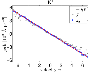
       (a) (b)

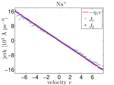
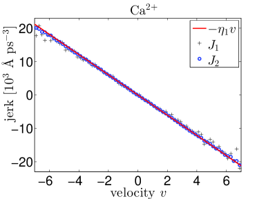
       (c) (d)

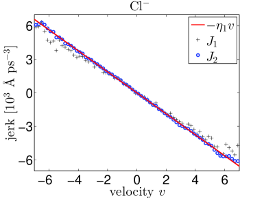
Figure 1: Comparison of the rate of change of acceleration (jerk) computed by all-atom MD simulations and by the coarse-grained model $(\ref{BDXeqAAA})$–$(\ref{BDZeqAAA})$. MD results are visualized using functions $J_{1}(v)$ (black crosses) and $J_{2}(v)$ (blue circles) defined by equation $(\ref{J1J2def})$. The result obtained by the coarse-grained model is given by formula $(\ref{Jcoarseeta1v})$ (red solid line). We consider (a) K⁺ ion; (b) Na⁺ ion; (c) Ca²⁺ ion and (d) Cl^- ion. Parameters are given in Tables 1 and 3.

where $p_{u}(u)$ is the steady state distribution of $U_{i}$ estimated from the same long time MD trajectory. As before, we use all three dimensions to calculate the averages $J(v,u)$ and $p_{u}(u)$. Function $J_{1}(v)$ (which gives jerk at the most likely value of $U_{i}$) is plotted using crosses and function $J_{2}(v)$, the average over $U_{i}$ variable, is plotted using circles in Figure 1. In order to compare all-atom MD simulations with the coarse-grained model (2)–(5), we calculate the corresponding jerk matrix $J(v,u)$ for the coarse-grained model. We denote by $p(v,u,z)$ the stationary distribution of the stochastic process (3)–(5), i.e. $p(v,u,z)\,\mbox{d}v\,\mbox{d}u\,\mbox{d}z$ is the probability that $V_{i}(t)\in[v,v+\mbox{d}v)$, $U_{i}(t)\in[u,u+\mbox{d}u)$ and $Z_{i}(t)\in[z,z+\mbox{d}v)$. Then the jerk matrix (29) of the coarse-grained model (2)–(5) is

$$J(v,u)=\int_{-\infty}^{\infty}\lim_{\tau\to 0}\frac{\langle U_{i}(t+\tau)-u\,|\,V_{i}(t)=v,U_{i}(t)=u,Z_{i}(t)=z\rangle}{\tau}\,p(v,u,z)\,\mbox{d}z.$$

Using (4), we rewrite it as

$$J(v,u)=\int_{-\infty}^{\infty}\left(-\eta_{1}v+z\right)\,p(v,u,z)\,\mbox{d}z.$$ (32)

The stationary distribution $p(v,u,z)$ of (3)–(5) is Gaussian with mean $[0,0,0]^{T}$ and stationary covariance matrix:

$$\frac{1}{2\eta_{1}\eta_{2}\eta_{3}}\left(\begin{matrix}\eta_{4}^{2}&0&0\\ 0&\eta_{1}\eta_{4}^{2}&0\\ 0&0&\eta_{1}\eta_{3}\eta_{4}^{2}\end{matrix}\right).$$

Consequently, equation (32) implies

$$J(v,u)=-\eta_{1}v.$$ (33)

In Figure 1, we plot (33) using the red solid line. The comparison with all atom MD results (circles and squares) is excellent for all four ions considered in this paper. In particular, we have shown that the coarse-grained model (2)–(5) provides a good description of the rate of change of acceleration (jerk) at the MD timescale. We make use of this property in Section 6 where we use the same time step ($\Delta t=10^{-3}$ ps) for both the coarse-grained model (2)–(5) and all-atom MD simulations. The coarse-grained model (2)–(5) can also be coupled with BD description (1), which uses much larger time steps, as we show in the next section.

5 From the coarse-grained model (2)–(5) to Brownian dynamics

Let us consider the three-variable subsystem (3)–(5) of the coarse-grained model. Denoting ${\mathbf{y}}_{i}=[V_{i},U_{i},Z_{i}]$, equations (3)–(5) can be written in vector notation as follows

$$\mbox{d}{\mathbf{y}}_{i}=B\,{\mathbf{y}}_{i}\,\mbox{d}t+{\mathbf{b}}\,\mbox{d}W_{i},$$ (34)

where matrix $B\in{\mathbb{R}}^{3\times 3}$ and vector ${\mathbf{b}}\in{\mathbb{R}}^{3}$ are given as

$$B=\left(\begin{matrix}0&1&0\\ -\eta_{1}&0&1\\ 0&-\eta_{3}&-\eta_{2}\end{matrix}\right)\qquad\mbox{and}\qquad{\mathbf{b}}=\left(\begin{matrix}0\\ 0\\ \eta_{4}\end{matrix}\right).$$ (35)

Let us denote the eigenvalues and eigenvectors of $B$ as $\lambda_{j}$ and ${\boldsymbol{\nu}}_{j}=[\nu_{1j},\nu_{2j},\nu_{3j}]$, $j=1,2,3$, respectively. The eigenvalues of $B$ are the solutions of the characteristic polynomial

$$\lambda^{3}+\eta_{2}\,\lambda^{2}+(\eta_{1}+\eta_{3})\lambda+\eta_{1}\eta_{2}=0.$$

Since $\eta_{1}$, $\eta_{2}$ and $\eta_{3}$ are positive parameters, we conclude that real parts of all three eigenvalues are negative and lie in interval $(-\eta_{2},0).$ Using the values of $\eta_{j}$, $j=1,2,3$, given in Table 3, we present the values of eigenvalues $\lambda_{j}$, $j=1,2,3,$ in Table 4.

$\lambda_{1}$ $\lambda_{2}$ $\lambda_{3}$ $t_{1}^{*}$ $t_{2}^{*}$ ​​​​ ion ​​​​ ​​​[ps^-1]​​​ ​​​[ps^-1]​​​ ​​​[ps^-1]​​​ ​​​[ps]​​​ ​​​[ps]​​​ ​​​​ K⁺ ​​​​ $\!\!\!-127.0$ ​​​ ​​​ $-12.75+27.58\,\mathbbm{i}$ ​​​ ​​​ $-12.75-27.58\,\mathbbm{i}$ ​​​ ​​​ $3.08\!\times\!10^{-2}$ ​​​ ​​​ $-9.39\!\times\!10^{-3}$ ​​​ ​​​​ Na⁺ ​​​​ ​​​ $-140.1$ ​​​ ​​​ $-12.99+47.47\,\mathbbm{i}$ ​​​ ​​​ $-12.99-47.47\,\mathbbm{i}$ ​​​ ​​​ $6.15\!\times\!10^{-3}$ ​​​ ​​​ $-2.35\!\times\!10^{-2}$ ​​​ ​​​​ Ca²⁺ ​​​​ ​​​ $-163.1$ ​​​ ​​​ $-13.58+57.84\,\mathbbm{i}$ ​​​ ​​​ $-13.58-57.84\,\mathbbm{i}$ ​​​ ​​​ $1.47\!\times\!10^{-3}$ ​​​ ​​​ $-2.48\!\times\!10^{-2}$ ​​​ ​​​​ Cl^- ​​​​ ​​​ $-162.9$ ​​​ ​​​ $-13.41+30.25\,\mathbbm{i}$ ​​​ ​​​ $-13.41-30.25\,\mathbbm{i}$ ​​​ ​​​ $2.50\!\times\!10^{-2}$ ​​​ ​​​ $-1.13\!\times\!10^{-2}$ ​​​

Table 4: Eigenvalues $\lambda_{j}$, $j=1,2,3$, of matrix $B$ defined by $(\ref{defBb})$ and time shifts $t_{1}^{*}$ and $t_{2}^{*}.$ Symbol $\mathbbm{i}$ denotes the imaginary unit.

The eigenvalues $\lambda_{j}$, $j=1,2,3$, are distinct. The general solution of the SDE system (34) can be written as follows [27]

$${\mathbf{y}}_{i}(t)=\Phi(t)\,{\mathbf{c}}+\Phi(t)\int_{0}^{t}\Phi^{-1}(s)\,{\mathbf{b}}\,\mbox{d}W_{i},$$ (36)

where ${\mathbf{c}}\in{\mathbb{R}}^{3}$ is a constant vector determined by initial conditions and matrix $\Phi(t)\in{\mathbb{R}}^{3\times 3}$ is given as $\Phi(t)=[\exp(\lambda_{1}t){\boldsymbol{\nu}}_{1}\;|\;\exp(\lambda_{2}t){\boldsymbol{\nu}}_{2}\;|\;\exp(\lambda_{3}t){\boldsymbol{\nu}}_{3}],$ i.e. each column is a solution of the ODE system $\mbox{d}{\mathbf{y}}_{i}=B\,{\mathbf{y}}_{i}\,\mbox{d}t$. Considering deterministic initial conditions, equation (36) implies that the process is Gaussian at any time $t>0$. Equations for means, variances and covariances then uniquely determine the distribution of ${\mathbf{y}}_{i}(t)$ for $t>0$. Equations for means can be written in the vector form as $\mbox{d}\langle{\mathbf{y}}_{i}\rangle=B\,\langle{\mathbf{y}}_{i}\rangle\,\mbox{d}t.$ Equations for variances and covariances are given in Section 3 as equations (9)–(12), (15), (17)–(20) and (22).

There are two important conclusions of the above analysis. First of all, eigenvalues $\lambda_{j}$, $j=1,2,3$, given in Table 4 satisfy

$$\lambda_{1}<\mbox{Re}\,\lambda_{2}=\,\mbox{Re}\lambda_{3}<0,$$

where Re denotes the real part of a complex number. There is a spectral gap between the first eigenvalue and the complex conjugate pair of eigenvalues. If we used this spectral gap, we could reduce the system to two evolution equations for times $t\gg 1/|\lambda_{1}|$. However, there is no spectral gap to reduce the system to Langevin dynamics (24)–(25). In particular, we again confirm our conclusion that a coarse-grained approximation of ion behaviour is not given in terms of Langevin dynamics. Our second conclusion is that on a picosecond time scale, we can assume stationarity in (34) to get

$$\mbox{d}X_{i} = \frac{\eta_{4}}{\eta_{1}\eta_{2}}\;\mbox{d}W_{i},\quad i=1,2,3.$$ (37)

Using (13), (21) and (23), we have

$$\frac{\eta_{4}}{\eta_{1}\eta_{2}}=\sqrt{2D}.$$

Consequently, equation (37) is equivalent to BD description (1). The convergence of (2)–(5) to the BD model is illustrated in Figure 2(a). We solve the system of 10 ODEs for variances and covariances given as equations (9)–(12), (15), (17)–(20) and (22). We consider (deterministic) zero initial conditions, i.e. $X_{i}(0)=V_{i}(0)=U_{i}(0)=Z_{i}(0)=0$. All moments are then initially equal to zero. We plot the mean square displacement $\langle X_{i}^{2}\rangle$ as a function of time. We compare it with the mean square displacement of BD model (1) which is given as $2Dt.$ We observe that there is an approximately constant shift, denoted $t_{1}^{*}$, between both solutions for times $t>0.2$ ps. We illustrate this further by plotting $\langle X_{i}^{2}(t+t_{1}^{*})\rangle$ in Figure 2(a). The values of shift $t_{1}^{*}$ for different ions estimated by solving the ODEs for second moments with zero initial conditions are given in Table 4.

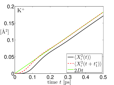
(a)                                                       (b)

Figure 2: (a) Comparison of the coarse-grained model $(\ref{BDXeqAAA})$–$(\ref{BDZeqAAA})$ and BD description $(\ref{BDSDE})$ for K⁺ ion. The mean square displacement computed by solving 10 ODEs $(\ref{V2eq})$–$(\ref{VZeq})$, $(\ref{UZeq})$, $(\ref{X2eq})$–$(\ref{XZeq})$ and $(\ref{Z2eq})$ with zero initial conditions (black solid line). The same curve shifted by the value of $t_{1}^{*}$ is plotted as a red dashed line. (b) Test of accuracy of the multiscale approach in $\Omega_{3}\cup\Omega_{4}\cup\Omega_{5}$ for K⁺ ion. Histogram obtained by simulating $10^{6}$ ions over time $10^{3}\,$ps is compared with the analytical result $(\ref{exsol106})$ (red solid line). Grey bars show the ion density in $\Omega_{3}$, the green bar shows the ion density in $\Omega_{4}$ and blue bars show the ion density in $\Omega_{5}$. Parameters are given in Tables 1 and 3.

Next, we show how the BD model (1) and the coarse-grained model (2)–(5) can be used in different parts of the computational domain. This coupling will form one component of multiscale methodology developed in Section 6. BD algorithms based on equation (1) have been implemented in a number of methods designed for spatio-temporal modelling of intracellular processes, including Smoldyn [28], MCell [29] and Green’s-function reaction dynamics [30]. Smoldyn discretizes (1) using a fixed BD time step $\Delta T$, i.e. it computes the time evolution of the position ${\mathbf{X}}\equiv{\mathbf{X}}(t)$ of each molecule by

$$X_{i}(t+\Delta t)=X_{i}(t)+\sqrt{2D\Delta T}\,\xi_{i},\qquad i=1,2,3,$$ (38)

where $[\xi_{1},\xi_{2},\xi_{3}]$ is a vector of normally distributed random numbers with zero mean and unit variance. We use discretization (38) of BD model (1) in this paper. BD time step $\Delta T$ has to be chosen much larger than the MD time step $\Delta t$. We use $\Delta T=0.5$ ps, but any larger time step would also work well. We could also use a variable time step, as implemented in the Green’s Function Reaction Dynamics [30].

In Section 6, we consider all-atom MD simulations in domain $\Omega\subset{\mathbb{R}}^{3}$. Our main goal is to design a multiscale approach which can compute spatio-temporal statistics with the MD-level of detail in relatively small subdomain $\Omega_{1}\subset\Omega$ by using BD model (38) in the most of the rest of the computational domain. This is achieved by decomposing domain $\Omega$ into five subdomains $\Omega_{j}$, $j=1,2,3,4,5$ (see equation (40) and discussion in Section 6). We use MD in $\Omega_{1}$, the coarse-grained model (2)–(5) in $\Omega_{3}$ and the BD model (38) in $\Omega_{5}$. The remaining two subdomains, $\Omega_{2}$ and $\Omega_{4}$, are two overlap (hand-shaking) regions where two different simulation approaches can be used at the same time [12, 31]. In the rest of this section, we focus on simulations in region $\Omega_{3}\cup\Omega_{4}\cup\Omega_{5}$ which concerns coupling the coarse-grained model (2)–(5) with the BD model (38). We use the coarse-grained model in $\Omega_{3}\cup\Omega_{4}$ and the BD model (38) in $\Omega_{4}\cup\Omega_{5}$. In particular, we use both models in the overlap region $\Omega_{4}$. Each particle which is initially in $\Omega_{3}$ is simulated according to (2)–(5) (discretized using time step $\Delta t$) until it enters $\Omega_{5}$. Then we use (38) to evolve the position of a particle (over BD time steps of length $\Delta T$) until it again enters $\Omega_{3}$ when we switch the description back from the BD model to the coarse-grained model. In order to do this, we have to initialize variables $V_{i}$, $U_{i}$ and $Z_{i}$, $i=1,2,3$. We use deterministic initial conditions, $V_{i}(0)=U_{i}(0)=Z_{i}(0)=0$, disccused above.

In Figure 2(b), we present an illustrative simulation where $\Omega_{3}\cup\Omega_{4}\cup\Omega_{5}={\mathbb{R}}^{3}$ for simplicity. We use $\Omega_{3}=(h,\infty)\times{\mathbb{R}}^{2}$, $\Omega_{4}=[-h,h]\times{\mathbb{R}}^{2}$ and $\Omega_{5}=(-\infty,-h)\times{\mathbb{R}}^{2}$, where $h=1\,$Å. We report averages over $10^{6}$ simulations of ions, half of them are initiated at ${\mathbf{X}}(0)=[h,0,0]$, i.e. they initially follow the coarse-grained model (2)–(5) with zero initial condition for other variables ($V_{i}(0)=U_{i}(0)=Z_{i}(0)=0$). The second half of ions are initiated at ${\mathbf{X}}(0)=[-h,0,0]$, i.e. they initially follow BD description (38). We plot the (marginal) distribution of ions along the first coordinate ($X_{1}$) at time $10^{3}\,$ps in Figure 2(b). The computed histogram is plotted using bins of length $2\,$Å, i.e. the overlap region $\Omega_{4}$ is equal to one bin (visualized as a green bar). Grey (resp. blue) bars show the density of ions in $\Omega_{3}$ (resp. $\Omega_{5}$). We compare our results with the analytical distribution computed for BD description (1) at time $t=10^{3}\,$ps given by

$$\varrho(x_{1})=\frac{10^{6}}{4\sqrt{\pi Dt}}\left(\exp\left[-\frac{(x_{1}-h)^{2}}{4Dt}\right]+\exp\left[-\frac{(x_{1}+h)^{2}}{4Dt}\right]\right).$$ (39)

The computed histogram compares well with (39), although we can observe a small error: the green bar is slightly taller than the corresponding value of (39). If we wanted to further improve the accuracy, we could take into account that there is time shift $t_{1}^{*}$, discussed above, introduced to the multiscale approach by using the deterministic initial conditions, $V_{i}(0)=U_{i}(0)=Z_{i}(0)=0$, for ions entering domain $\Omega_{3}$. Another possibility is to sample the initial condition for $V_{i},$ $U_{i}$ and $Z_{i}$ from a suitable distribution. If we use the stationary distribution of subsystem (3)–(5), then $\langle V_{i}^{2}\rangle$ does not evolve and is equal to

$$\langle V_{i}^{2}\rangle=\frac{\eta_{4}^{2}}{2\eta_{1}\eta_{2}\eta_{3}}.$$

Substituting this constant for $\langle V_{i}^{2}\rangle$ into (18), the system of 10 ODEs for second moments of (2)–(5) simplifies to 4 ODEs (17)–(20). Solving system (17)–(20) with zero initial conditions (assuming $X_{i}(0)=0$), we can again compute the mean square displacement. As in Figure 2(a), it can be shifted in time to better match with the BD result, $2Dt$. We denote this time shift as $t_{2}^{*}$. Its values are given in Table 4. We observe that $t_{2}^{*}$ is negative and $t_{1}^{*}$ is positive for all four ions considered in Table 4. Both time shifts $t_{1}^{*}$ and $t_{2}^{*}$ (together with optimizing size $h$ of the overlap region) could be used to further improve the accuracy of multiscale simulations in $\Omega_{3}\cup\Omega_{4}\cup\Omega_{5}$ [12]. However, our main goal is to introduce a multiscale approach which can use all-atom MD simulations in $\Omega_{1}$. Since MD simulations are computationally intensive, we will only consider 100 realizations of the multiscale method in Section 6. In particular, the Monte Carlo error will be larger than the error observed in Figure 2(b). Thus, we can use the above approach in $\Omega_{3}\cup\Omega_{4}\cup\Omega_{5}$ without introducing observable errors in the multiscale method developed in the next section.

6 Coupling all-atom MD and BD

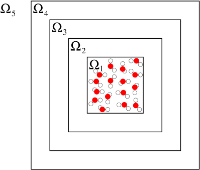
Ion simulated using all-atom MD                                                                   in $\Omega_{1}$.
                                                                  Ion described by the coarse-grained                                                                   model (2)–(5) in $\Omega_{2}$, $\Omega_{3}$ and $\Omega_{4}$.
                                                                  Ion described by BD model (38)                                                                   in $\Omega_{4}$ and $\Omega_{5}$.
                                                                  If an ion is in $\Omega_{1}$ or $\Omega_{2}$, then water                                                                   molecules are simulated using                                                                   all-atom MD in $\Omega_{1}$.

Figure 3: Schematic of multiscale set up. Note that the schematic is drawn in two spatial dimensions to enable better visualization, but all models are formulated and simulated in three spatial dimensions.

Let us consider all-atom MD in domain $\Omega\subset{\mathbb{R}}^{3}$ which is so large that direct MD simulations would be too computationally expensive. Let us assume that a modeller only needs to consider the MD-level of detail in a relatively small subdomain $\Omega_{1}\subset\Omega$ while, in the rest of the computational domain, ions are transported by diffusion and BD description (1) is applicable. For example, domain $\Omega_{1}$ could include binding sites for ions or (parts of) ion channels. In this paper, we do not focus on a specific application. Our goal is to show that the coarse-grained model (2)–(5) is an intermediate model between all-atom MD and BD which enables the use of both methods during the same dynamic simulation. To achieve this, we decompose domain $\Omega$ into five subdomains, denoted $\Omega_{j}$, $j=1,2,3,4,5,$ see Figure 3. These sets are considered pairwise disjoint (i.e. $\Omega_{i}\cap\Omega_{j}=\emptyset$ for $i\neq j$) and

$$\Omega=\Omega_{1}\cup\Omega_{2}\cup\Omega_{3}\cup\Omega_{4}\cup\Omega_{5}.$$ (40)

In our illustrative simulations, we consider the behaviour of one ion. If the ion is in subdomain $\Omega_{1}$, then we use all-atom MD simulations as described in Section 2. In particular, the force between the ion and a water molecule is obtained by differentiating potential (6), provided that the distance between the ion and the water molecule is less than the cutoff distance ($L/2$). Let us denote the force exerted by the ion on the water molecule by ${\mathbf{F}}_{iw}(r_{i0},r_{i1},r_{i2})$, where $r_{i0}$ (resp., $r_{i1}$ and $r_{i2}$) is the distance between the ion and the oxygen site (resp., the first and second hydrogen sites) on the water molecule. We use periodic boundary conditions for water molecules in $\Omega_{1}$.

Whenever the ion leaves $\Omega_{1}$, it enters $\Omega_{2}$ where we simulate its behaviour using the coarse-grained model (2)–(5). We still simulate water molecules in $\Omega_{1}$ and we allow them to experience additional forces exerted by the ion which is present in $\Omega_{2}$. These forces have the same functional form, ${\mathbf{F}}_{iw}$, as in MD, but they have modified arguments as follows

$${\mathbf{F}}_{iw}\big{(}r_{i0}+\omega\,\mbox{dist}({\mathbf{X}},\Omega_{1}),r_{i1}+\omega\,\mbox{dist}({\mathbf{X}},\Omega_{1}),r_{i2}+\omega\,\mbox{dist}({\mathbf{X}},\Omega_{1})\big{)},$$ (41)

where $\omega\geq 0$ is a parameter and $\mbox{dist}({\mathbf{X}},\Omega_{1})$ is the (closest) distance between the ion at position ${\mathbf{X}}$ and subdomain $\Omega_{1}$. If the ion is in region $\Omega_{3}\cup\Omega_{4}\cup\Omega_{5}$, then water molecules in $\Omega_{1}$ are no longer simulated. We use the coarse-grained model (2)–(5) to simulate the ion behaviour in $\Omega_{3}$ and the BD model (38) in $\Omega_{5}$. Overlap region $\Omega_{4}$ is used to couple these simulation methods as explained in Section 5.

In Section 5, we have already presented illustrative simulations to validate the multiscale modelling strategy chosen in region $\Omega_{3}\cup\Omega_{4}\cup\Omega_{5}$. Next, we focus on testing and explaining the multiscale approach chosen to couple region $\Omega_{1}$ with $\Omega_{2}$. The key idea is given by force term (41) which is used for MD simulations of water molecules in $\Omega_{1}$ when an ion is in $\Omega_{2}$. This force term has two important properties:

(i) If an ion is on the boundary of $\Omega_{1}$, i.e. ${\mathbf{X}}\in\partial\Omega_{1}$, then $\mbox{dist}({\mathbf{X}},\Omega_{1})=0$ and force (41) is equal to force term ${\mathbf{F}}_{iw}(r_{i0},r_{i1},r_{i2})$ used in $\Omega_{1}$.

(ii) If $\omega\,\mbox{dist}({\mathbf{X}},\Omega_{1})\geq L/2$, then force (41) is equal to zero.

Property (i) implies that formula (41) continuously extends the force term used in MD. In particular, water molecules do not experience abrupt changes of forces when the ion crosses boundary $\partial\Omega_{1}.$ Property (ii) is a consequence of the cutoff distance used (together with the reaction field correction [1]) to treat long-range interactions. In our illustrative simulations, we use

$$\Omega_{1}=\left[-\frac{L}{2},\frac{L}{2}\right]^{3}\qquad\quad\mbox{and}\qquad\quad\Omega_{2}=\left[-\frac{L}{2}-\frac{L}{2\omega},\frac{L}{2}+\frac{L}{2\omega}\right]^{3}\setminus\Omega_{1}.$$ (42)

Property (ii) implies that extra force (41) is equal to zero on boundary $\partial\Omega_{2}\setminus\partial\Omega_{1}$ which is the boundary between regions $\Omega_{2}$ and $\Omega_{3}$. This is consistent with the assumption that ions in region $\Omega_{3}\cup\Omega_{4}\cup\Omega_{5}$ do not interact with water molecules in region $\Omega_{1}$.

If an ion is in $\Omega_{1}$, we use all-atom MD as formulated in Section 2. Periodic boundary conditions are implemented in MD simulations. Water molecules are subject to forces exerted by the ion at its real position ${\mathbf{X}}$ in $\Omega_{1}$, but also by its copies at periodic locations ${\mathbf{X}}+(iL,jL,kL)$ where $i,j,k\in{\mathbb{Z}}.$ When the ion moves to $\Omega_{2}$, one of its copies is in $\Omega_{1}$. Force term (41) is designed in such a way, that the strength of interaction decreases (for every copy of the ion) with the distance, $\mbox{dist}({\mathbf{X}},\Omega_{1})$, between the real position of the ion and $\Omega_{1}$. In particular, force term (41) ensures that there are continuous changes of all forces when the ion moves between regions $\Omega_{1}$, $\Omega_{2}$ and $\Omega_{3}.$

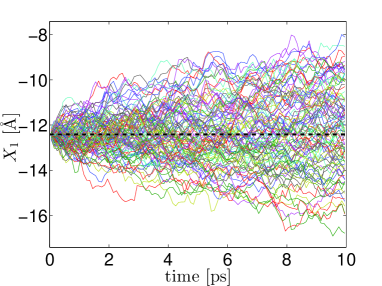
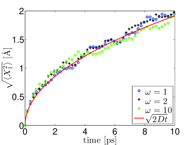
(a)                                                       (b)

Figure 4: (a) One hundred realizations of a multiscale simulation of K⁺ ion initiated at $[-L/2,0,0]$. We plot $X_{1}$ coordinate as a function of time. Ion is described by all-atom MD for $X_{1}\geq-L/2$ and by the coarse-grained model $(\ref{BDXeqAAA})$–$(\ref{BDZeqAAA})$ for $X_{1}<-L/2$. The boundary between $\Omega_{1}$ and $\Omega_{2}$ is visualized using the black dashed line. We use $\omega=1$ in $(\ref{iwforce})$. (b) The mean square displacement in the first coordinate of K⁺ ion simulated in $\Omega_{1}\cup\Omega_{2}$ and computed as the average of $100$ realizations for $\omega=1$ (blue circles), $\omega=2$ (black crosses) and $\omega=10$ (green squares).

In Figure 4, we present results of simulations of K⁺ ion in region $\Omega_{1}\cup\Omega_{2}$. We consider 100 realizations of a multiscale simulation with one ion. Its initial position is ${\mathbf{X}}(0)=[-L/2,0,0]$ which lies on boundary $\partial\Omega_{1}$. We simulate each realization for time 10 ps which is short enough that all trajectories stay inside the ball of radius $L/2$ centred at ${\mathbf{X}}(0)$. Then $X_{1}$-coordinate of the trajectory determines whether the ion is in $\Omega_{1}$ or $\Omega_{2}$. If $X_{1}(t)\geq-L/2$, then the ion is in $\Omega_{1}$ and it is simulated using all-atom MD. If $X_{2}(t)<-L/2$, then the ion is in $\Omega_{2}$ and evolves according to the coarse-grained model (2)–(5). In Figure 4(a), we use (41) with $\omega=1$ and plot $X_{1}$ coordinates of all 100 realizations. We observe that the computed trajectories spread on both sides of boundary $\partial\Omega_{1}$ (dashed line) without any significant bias. The mean square displacement is presented in Figure 4(b) for three different values of $\omega$. The results compare well with $(2Dt)^{1/2}$ which is the mean square displacement of one coordinate of the diffusion process.

We conclude with illustrative simulations which are coupling all-atom MD with BD. We use domain $\Omega\in{\mathbb{R}}^{3}$ decomposed into five regions as in equation (40), where $\Omega_{1}$ and $\Omega_{2}$ are given by (42), and

$$\Omega_{3} = \left[-\frac{L}{2}-\frac{L}{2\omega}-h_{1},\frac{L}{2}+\frac{L}{2\omega}+h_{1}\right]^{3}\setminus(\Omega_{1}\cup\Omega_{2}),$$ (43)

$$\Omega_{4} = \left[-\frac{L}{2}-\frac{L}{2\omega}-h_{1}-h_{2},\frac{L}{2}+\frac{L}{2\omega}+h_{1}+h_{2}\right]^{3}\setminus(\Omega_{1}\cup\Omega_{2}\cup\Omega_{3}),\qquad$$ (44)

$$\Omega_{5} = {\mathbb{R}}^{3}\setminus(\Omega_{1}\cup\Omega_{2}\cup\Omega_{3}\cup\Omega_{4}),$$ (45)

where $\omega=10$, $h_{1}=L/20$ and $h_{2}=L/10$. Then the BD domain is $\Omega_{5}={\mathbb{R}}^{3}\setminus[-7L/10,7L/10]^{3}$. We place an ion at the origin (centre of MD domain $\Omega_{1}$), i.e. ${\mathbf{X}}(0)=[0,0,0],$ and we simulate each trajectory until it reaches the distance $4L=99.32\,$Å from the origin. Let ${\cal T}(r)$ be the time when a trajectory first reaches distance $r$ from the origin.

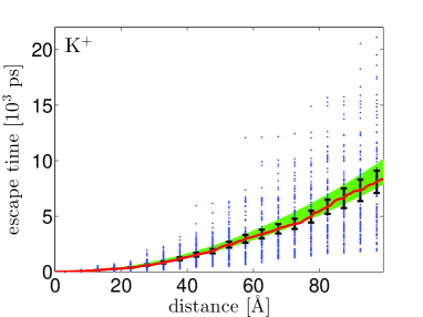
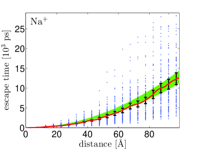
(a)                                                       (b)

Figure 5: Escape time ${\cal T}(r)$ to reach distance $r$ from the origin computed by the multiscale method. We consider (a) K⁺ ion; and (b) Na⁺ ion. We plot escape times for individual realizations (blue points), the mean escape time estimated from $100$ realizations (red solid line) and the theoretical $95$% confidence interval $(\ref{theorconfinterval})$ (green area). We use $\omega=10$ in $(\ref{iwforce})$.

In Figure 5, we plot escape time ${\cal T}(r)$ as a function of distance $r$. We plot the value of ${\cal T}(r)$ for each realization as a blue point. The largest computed escape times (for $r=4L$) are $38,506\,$ps for K⁺ and $47,212\,$ps for Na⁺. They are outside the range of panels in Figure 5, but the majority of data poins are included in this figure. We also plot average $\langle{\cal T}(r)\rangle$ (red solid line) together with 95% confidence intervals. They are compared with theoretical results obtained for the BD model (1). The escape time distribution for the BD model (1) has mean equal to $\langle{\cal T}(r)\rangle=L^{2}/(6D)$ and standard deviation $L^{2}/(3\sqrt{10}\,D).$ The corresponding theoretical 95% confidence interval (for 100 samples) is

$$\left(\frac{L^{2}}{6D}-1.96\frac{L^{2}}{30D},\,\frac{L^{2}}{6D}+1.96\frac{L^{2}}{30D}\right).$$ (46)

This interval is visualized as the green area in Figure 5. We note that it would be relatively straightforward to continue the presented multiscale computation and simulate ion diffusion in domains covering the whole cell. The most computationally intensive part is all-atom MD simulation in $\Omega_{1}\cup\Omega_{2}$. However, once the ion enters $\Omega_{5}$, we can compute its trajectory very efficiently. We could further increase the BD time step in parts of $\Omega_{5}$ which are far away from $\Omega_{4}$, or we could use event-based algorithms, like Green’s-function reaction dynamics [30] or First-passage kinetic Monte Carlo method [32], to compute the ion trajectory in region $\Omega_{5}$.

7 Discussion

In this paper, we have introduced and studied the coarse-grained model (2)–(5) of an ion in aqueous solution. We have parameterized this model using all-atom MD simulations for four ions (K⁺, Na⁺, Ca²⁺ and Cl^-) and showed that this model provides an intermediate description between all-atom MD and BD simulations. It can be used both with MD time step $\Delta t$ (to couple it with all-atom MD simulations) and BD time step $\Delta T$ (to couple it with BD description (1)). In particular, the coarse-grained model enables multiscale simulations which use all-atom MD and BD in different parts of the computational domain.

In Section 6, we have illustrated this multiscale methodology using a first passage type problem where we have reported the time taken by an ion to reach a specific distance. Possible applications of this multiscale methodogy include problems where a modeller considers all-atom MD in several different parts of the cell (for example, close to binding sites or ion channels) and wants to use efficient BD simulations to transport ions by diffusion between regions where MD is used. The proposed approach thus enables the inclusion of MD-level of detail in computational domains which are much larger than would be possible to study by direct MD simulations.

Although the illustrative simulations in Section 6 are reported over distances of the order of $10^{2}$ Å, this is not a restriction of the method. Most of the computational time is spent by considering all-atom MD in $\Omega_{1}\cup\Omega_{2}$. BD uses much larger time step which enables us to futher extend BD region $\Omega_{5}$ (and consequently, the original domain $\Omega$). Moreover, if we are far away from MD domain $\Omega_{1}$, we can further increase the efficiency of BD simulations by using different BD time steps in different parts of the BD subdomain $\Omega_{5}$ [12], or by using event-based BD algorithms [30, 32]. The computational intensity of BD simulations can be further decreased by using multiscale methods which efficiently and accurately combine BD models with lattice-based (compartment-based) models [33, 34]. Such a strategy have been previously used for modelling intracellular calcium dynamics [3, 7] or actin dynamics in filopodia [35], and enables us to extend both temporal and spatial extent of the simulation.

In the literature, MD methods have been used to estimate parameters of BD simulations of ions [36]. There has also been a lot of progress in systematic coarse-graining of MD simulations [37]. The approach presented in this paper not only uses all-atom MD simulations to estimate parameters of a coarser description, but it also designs a multiscale approach where both methods are used during the same simulation. Methods which adaptively change the resolution of MD on demand have been previously reported in [38, 39]. They include algorithms which couple all-atom MD with coarse-grained MD. The coarse-grained model developed in this work does not include any water molecules and has different application areas. One of them is modelling of calcium induced calcium release through IP₃R channels [3] which is discussed as a motivating example in Introduction. MD simulations in this paper use the three-site SPC/E model of water. An open question is to extend our observations and analysis to other MD models of water, which include both more detailed water models with additional sites [16, 17] and coarse-grained MD models of water [40].

References

- [1] S. Koneshan, J. Rasaiah, M. Lynden-Bell, and S. Lee. Solvent structure, dynamics and ion mobility in aqueous solutions at 25C. Journal of Physical Chemistry B, 102:4193–4204, 1998.
- [2] M. Kohagen, P. Mason, and P. Jungwirth. Accurate description of calcium solvation in concentrated aqueous solutions. Journal of Physical Chemistry B, 118:7902–7909, 2014.
- [3] U. Dobramysl, S. Rüdiger, and R. Erban. Particle-based multiscale modeling of intracellular calcium dynamics. submitted, available as http://arxiv.org/abs/1504.00146, 2015.
- [4] B. Corry, S. Kuyucak, and S. Chung. Test of continuum theories as models of ion channels. II. Poisson-Nernst-Planck theory versus Brownian dynamics. Biophysical Journal, 78:2364–2381, 2000.
- [5] R. Erban, S. J. Chapman, and P. Maini. A practical guide to stochastic simulations of reaction-diffusion processes. 35 pages, available as http://arxiv.org/abs/0704.1908, 2007.
- [6] B. Leimkuhler and C. Matthews. Molecular Dynamics, volume 39 of Interdisciplinary Applied Mathematics. Springer, 2015.
- [7] M. Flegg, S. Rüdiger, and R. Erban. Diffusive spatio-temporal noise in a first-passage time model for intracellular calcium release. Journal of Chemical Physics, 138:154103, 2013.
- [8] R. Erban and S. J. Chapman. Stochastic modelling of reaction-diffusion processes: algorithms for bimolecular reactions. Physical Biology, 6(4):046001, 2009.
- [9] J. Lipkova, K. Zygalakis, J. Chapman, and R. Erban. Analysis of Brownian dynamics simulations of reversible bimolecular reactions. SIAM Journal on Applied Mathematics, 71(3):714–730, 2011.
- [10] T. Shinohara, T. Michikawa, M. Enomoto, J. Goto, M. Iwai, T. Matsu-ura, H. Yamazaki, A. Miyamoto, A. Suzuki, and K. Mikoshiba. Mechanistic basis of bell-shaped dependence of inositol 1,4,5-trisphosphate receptor gating on cytosolic calcium. Proceedings of the National Academy of Sciences USA, 108(37):15486–15491, 2011.
- [11] I. Serysheva. Toward a high-resolution structure of IP3R channel. Cell Calcium, 56:125–132, 2014.
- [12] R. Erban. From molecular dynamics to Brownian dynamics. Proceedings of the Royal Society A, 470:20140036, 2014.
- [13] H. Berendsen, J. Postma, W. Van Gunsteren, and J. Hermans. Interaction models for water in relation to protein hydration. In B. Pullman, editor, Intermolecular Forces, pages 331–342. D. Reidel Publishing Company, 1981.
- [14] H. Berendsen, J. Grigera, and T. Straatsma. The missing term in effective pair potentials. Journal of Physical Chemistry, 91(24):6169–6271, 1987.
- [15] W. Jorgensen, J. Chandrasekhar, J. Madura, R. Impey, and M. Klein. Comparison of simple potential functions for simulating liquid water. Journal of Chemical Physics, 79(2):926–935, 1983.
- [16] D. Huggins. Correlations in liquid water for the TIP3P-Ewald, TIP4P-2005, TIP5P-Ewald, and SWM4-NDP models. Journal of Chemical Physics, 136(6):064518, 2012.
- [17] P. Mark and L. Nilsson. Structure and dynamics of the TIP3P, SPC, and SPC/E water models at 298 K. Journal of Physical Chemistry A, 105(43):9954–9960, 2001.
- [18] S. Lee and J. Rasaiah. Molecular dynamics simulation of ion mobility. 2. alkali metal and halide ions using the SPC/E model for water at 25C. Journal of Physical Chemistry, 100:1420–1425, 1996.
- [19] H. Andersen. Rattle: a “velocity" version of the Shake algorithm for molecular dynamics calculations. Journal of Computational Physics, 52:24–34, 1983.
- [20] S. Nosé. A unified formulation of the constant temperature molecular dynamics methods. Journal of Chemical Physics, 81:511–519, 1984.
- [21] W. Hoover. Canonical dynamics: Equilibrium phase-space distributions. Physical Review E, 31(3):1695–1697, 1985.
- [22] L. Perera, U. Essmann, and M. Berkowitz. Effect of the treatment of long-range forces on the dynamics of ions in aqueous solutions. Journal of Chemical Physics, 102(1):450–456, 1995.
- [23] T. Nymand and P. Linse. Ewald summation and reaction-field methods for potentials with atomic charges, dipoles and polarizabilities. Journal of Chemical Physics, 112(14):6152–6160, 2000.
- [24] R. Holley. The motion of a heavy particle in an infinite one dimensional gas of hard spheres. Zeitschrift für Wahrscheinlichkeitstheorie und Verwandte Gebiete, 17:181–219, 1971.
- [25] D. Dürr, S. Goldstein, and J. Lebowitz. A mechanical model of Brownian motion. Communications in Mathematical Physics, 78:507–530, 1981.
- [26] J. Dunkel and P. Hänggi. Relativistic Brownian motion: From a microscopic binary collision model to the Langevin equation. Physical Review E, 74(5):051106, 2006.
- [27] X. Mao. Stochastic Differential Equations and Applications. Horwood Publishing, Chichester, UK, 2007.
- [28] S. Andrews and D. Bray. Stochastic simulation of chemical reactions with spatial resolution and single molecule detail. Physical Biology, 1:137–151, 2004.
- [29] J. Stiles and T. Bartol. Monte Carlo methods for simulating realistic synaptic microphysiology using MCell. In E. Schutter, editor, Computational Neuroscience: Realistic Modeling for Experimentalists, pages 87–127. CRC Press, 2001.
- [30] J. van Zon and P. ten Wolde. Green’s-function reaction dynamics: a particle-based approach for simulating biochemical networks in time and space. Journal of Chemical Physics, 123:234910, 2005.
- [31] B. Franz, M. Flegg, J. Chapman, and R. Erban. Multiscale reaction-diffusion algorithms: PDE-assisted Brownian dynamics. SIAM Journal on Applied Mathematics, 73(3):1224–1247, 2013.
- [32] T. Opplestrup, V. Bulatov, A. Donev, M. Kalos, G. Gilmer, and B. Sadigh. First-passage kinetic Monte Carlo method. Physical Review E, 80(6):066701, 2009.
- [33] M. Flegg, J. Chapman, and R. Erban. The two-regime method for optimizing stochastic reaction-diffusion simulations. Journal of the Royal Society Interface, 9(70):859–868, 2012.
- [34] M. Robinson, S. Andrews, and R. Erban. Multiscale reaction-diffusion simulations with Smoldyn. Bioinformatics, 31(14):2406–2408, 2015.
- [35] R. Erban, M. Flegg, and G. Papoian. Multiscale stochastic reaction-diffusion modelling: application to actin dynamics in filopodia. Bulletin of Mathematical Biology, 76(4):799–818, 2014.
- [36] T. Allen, S. Kuyucak, and S. Chung. Molecular dynamics estimates of ion diffusion in model hydrophobic and KcsA potassium channels. Biophysical Chemistry, 86:1–14, 2000.
- [37] M. Saunders and G. Voth. Coarse-graining methods for computational biology. Annual Review of Biophysics, 42:73–93, 2013.
- [38] M. Praprotnik, L. Delle Site, and K. Kremer. Multiscale simulation of soft matter: From scale bridging to adaptive resolution. Annual Review of Physical Chemistry, 59:545–571, 2008.
- [39] S. Nielsen, R. Bulo, P. Moore, and B. Ensing. Recent progress in adaptive multiscale molecular dynamics simulations of soft matter. Physical Chemistry Chemical Physics, 12(39):12401–12414, 2010.
- [40] M. Praprotnik, S. Matysiak, L. Delle Site, K. Kremer, and C. Clementi. Adaptive resolution simulation of liquid water. Journal of Physics: Condensed Matter, 19:292201, 2007.