On the Convergence of SGD Training of Neural Networks

Abstract

Neural networks are usually trained by some form of stochastic gradient descent (SGD)). A number of strategies are in common use intended to improve SGD optimization, such as learning rate schedules, momentum, and batching. These are motivated by ideas about the occurrence of local minima at different scales, valleys, and other phenomena in the objective function. Empirical results presented here suggest that these phenomena are not significant factors in SGD optimization of MLP-related objective functions, and that the behavior of stochastic gradient descent in these problems is better described as the simultaneous convergence at different rates of many, largely non-interacting subproblems.

1 Introduction

An one hidden layer multi-layer perceptron (MLP) is a nonlinear discriminant function

$$y=f_{\theta}(x)=\sigma(b+B\cdot\sigma(a+A\cdot x))$$

Here, the parameters $\theta$ are two vectors $a,b$ and two matrices $A,B$ , and $\sigma(...)$ is the element-wise sigmoid function of a vector.

These parameters are usually optimized by stochastic gradient descent, minimizing some objective function involving $y$ and the ground truth classification information. Let us call the objective function $C(\theta)$ . Much effort has been invested in coming up with efficient ways of performing this optimization or stochastic gradient descent[2, 7, 5, 6, 1].

Generally, $f_{\theta}$ is thought to be a function that has many local minima. Indeed, local minima are frequently observed in training small neural networks on problems like XOR, parity, and spiral problems. Much effort in the literature has been expended on ways to train despite the existence of such local minima[4, 8, 3].

Furthermore, any single local minimum gives rise to many more local minima because of symmetries of $f_{\theta}$ in its parameter vector (e.g., corresponding permutations of the rows of $A$ and the columns of $B$ yield the same classifier). Commonly, $C(\theta)$ is also thought to have a hierarchy of minima at different scales. These assumptions have yielded a number of common strategies for neural network training. For example, momentum is intended to smooth out local minima at small scales, and learning rate schedules are supposed to cope with a hierarchy of minima at different scales, in a way similar to simulated annealing.

Although these assumptions about the objective function are commonly made, they have received little empirical testing. That is in part because observing the convergence of MLPs in weight space is difficult because many different weight settings give equivalent outputs. In addition, it is difficult to explore the very high dimensional weight space of MLPs.

Here, we examine the question of how stochastic gradient descent optimization proceeds for MLPs with two simple approaches:

• We trace $C(\theta)$ over time as optimization proceeds for multiple different starting points.

• Instead of comparing the $\theta$ parameters, which are beset by complicated symmetries, we use a collection of test set samples $\{\xi_{1},...\xi_{N}\}$ and compute the corresponding vector $\tau(\theta)=(f_{\theta}(\xi_{1}),...,f_{\theta}(\xi_{N}))$. For two weight vectors $\theta$ and $\theta^{\prime}$ to be similar under symmetries, it is necessary (but not sufficient) for $\tau(\theta)\approx\tau(\theta^{\prime})$.

If the standard view of stochastic gradient descent (SGD) optimization of neural networks is correct, i.e., if there are numerous local minima, then the following predictions would hold true:

• For a given learning rate, SGD optimization would continue until the learning rate is too large and the search simply moves around in a random walk within the basin surrounding the local minimum.

• For a given learning rate, the parameter space of $\theta$ should be partitioned into regions, each of which corresponds to the basin surrounding a local minimum at the scale corresponding to the learning rate.

• We should be able to find multiple different starting points in parameter space that converge to the same basin surrounding a local minimum at a particular scale.

Note that for these predictions, the necessary-but-not-sufficient aspect of $\tau$-equivalence of parameters is not a problem. That is, the fact that $\tau$-equivalence may count some parameter vectors as equivalent that are, in fact, not equivalent does not invalidate any of these predictions; they hold true under both $\tau$-equivalence of parameters and true equivalence.

In fact, there are two different notions of parameter equivalence we use in the experiments below. The first is $\tau$-equivalence as defined above, namely a vector of discriminant function values predicted by the neural network on the test set. The second, let’s call it $\kappa$-equivalence replaces the discriminant functions with the class predictions for each test set sample. Under that weaker notion of equivalence, two sets of parameters are equivalent if they make the same classifications on the test set.

All the experiments reported below were carried out using the Torch machine learning library on the deskewed MNIST dataset using a one hidden layer MLP with 100 hidden units. The first 1000 samples of the official test set were used as the test set for predicting the $\tau$ and $\kappa$ vectors. All dimensionality reductions use the multidimensional scaling implementation from scikits-learn.

2 Large Scale Convergence

The initial experiment consisted of training 100 networks over 20 epochs. The results are shown in Figure 1. We can see that both discriminant functions and classification vectors over the test set start off in one region of space and then generally converge towards each other. The fact that the initial $\tau$ vectors appear to be much more diverse than the initial $\kappa$ vectors is a result of the nonlinearity implied by the argmax function that converts the discriminant function into classifications. That is, during the first epoch, the predictions $f_{\theta}(x)$ are all close to 0.5, but the use of the argmax function converts these very similar discriminant function values into wildly different classification results.

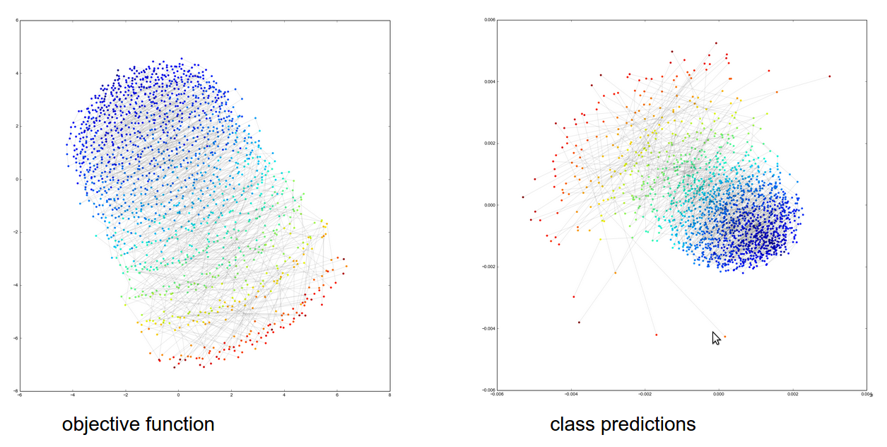
Figure 1: $\tau$ and $\kappa$ predictions for 100 networks over time using multidimensional scaling. Training epochs are indicated by color (from red to blue).

The natural next step is to visualize the space of paths after the effects of the initial training have worn off. This is shown in Figure 2. At first glance, this figure appears to show a large number of local minima, with each network stuck inside its own local minimum. However, in fact, what this image shows is a top down projection of a number of SGD paths that are all converging towards the center.

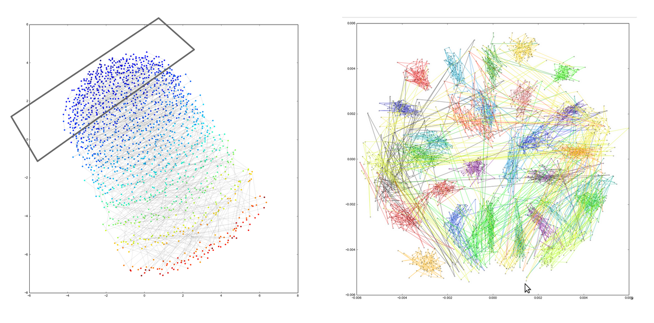
Figure 2: Paths in parameter space after initial training. At first glance, this appears to show multiple searches in local minima, but actually, each of the apparent local minima represents a path that slowly converges towards the center of the figure.

We can see this much more easily if we follow a smaller number of SGD paths, as shown in Figure 3. Now it is obvious that the paths are not, in fact, stuck in local minima, but that they are still all making progress towards a common optimum. To help with understanding the right panel of Figure 2, the equivalent perspective is shown on the right in Figure 3.

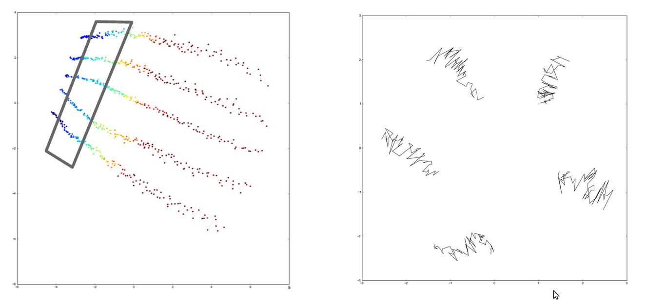
Figure 3: A small number of paths analyzed in the same way as Figure 2. Now it is clear that none of the paths are stuck in local minima, and instead keep making progress towards a common minimum near the top left of the plot. The right hand side shows a slice through these paths, which are now converting roughly towards the center.

We find the same result if we look at the $\kappa$ function instead of the $\tau$ function.

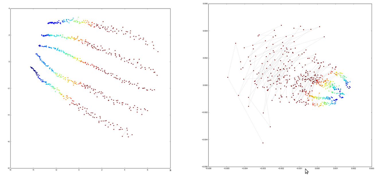
Figure 4: The same analysis as in Figure 3, but using class labels ( $\tau$-equivalence) instead of discriminant function values.

The above experiments do not suggest the existence of local minima. In fact, SGD training proceeds towards a common final minimum smoothly and steadily along separate paths; each path “remembers” the initial conditions, the random set of training weights that it was originally trained with. There is no sign of local minima at all. This is quite amazing if we recall that the classification error across these figures goes from around 90% to below 1%.

To push these experiments to their extremes, Figure 6 shows the $\tau$-functions of the parameters for epochs 50-500 for two networks, using a learning rate of 5 (a very high learning rate). Again, we see that each network steadily learns, but makes slower and slower progress as time goes on. There is no evidence of getting stuck in local minima, no evidence of minima at different scales (which would show up as “bouncing around” in weight space). Furthermore, the separation of the two networks in parameter space is large compared to the size of the updates. Even over 500 epochs of training and at a final error rate of around 0.15%, both networks retain a memory of the initial weight choices.

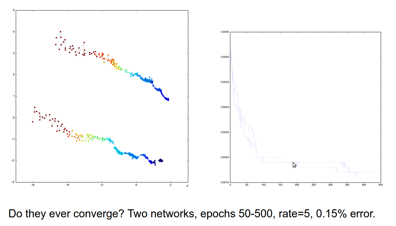
Figure 5: Pushing two networks out over very long periods (epochs 50-500, learning rate = 5, final training set error is 0.15%). The networks retain a memory of their initial conditions over 500 epochs and never reach a local minimum, common or otherwise, despite having very similar classification error rates.

One of the mechanisms proposed for improving convergence of stochastic gradient descent is smoothing via momentum of batching. The effect of this can be seen in Figure 6. We can see that batched updates do indeed lead to a much smoother optimization path initially, but in the long run, both paths smooth out and converge gradually. There is no evidence that batching or averaging avoids “bouncing around in local minima” or helps the MLP converge faster or better.

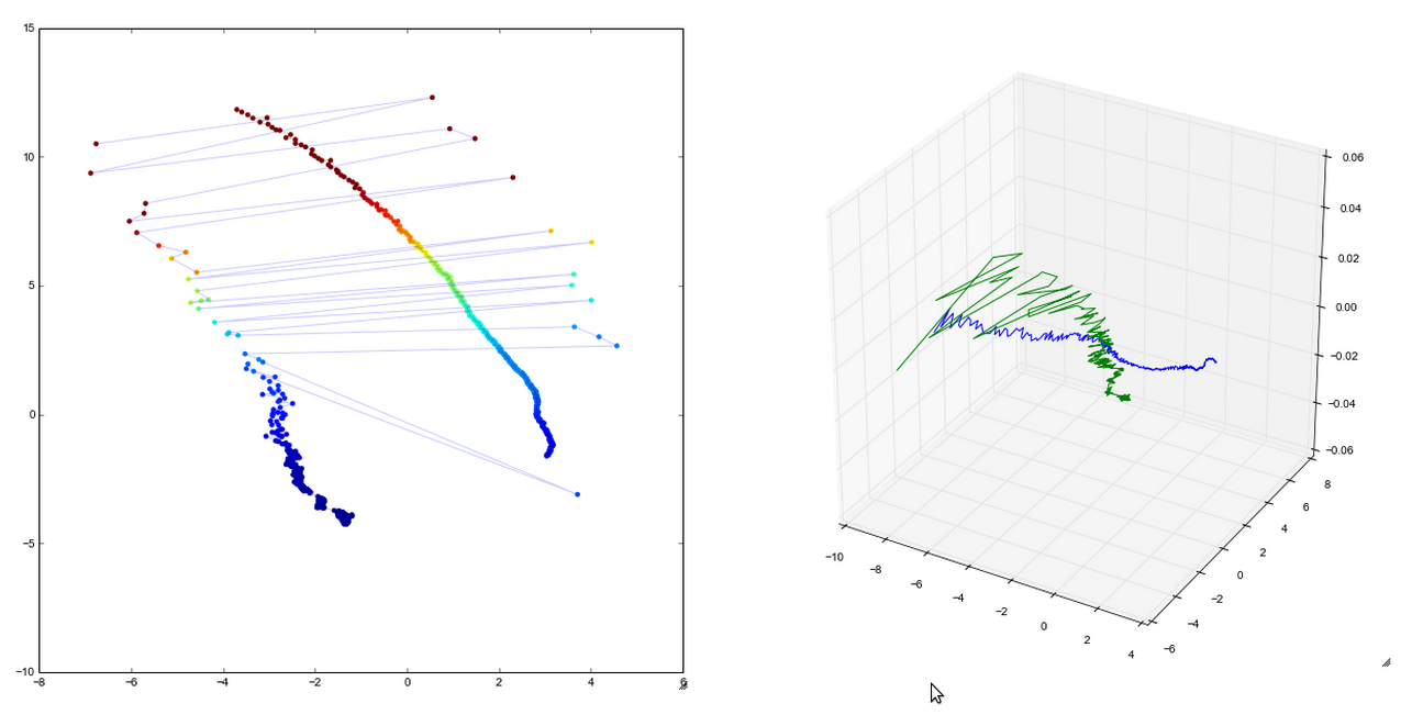
Figure 6: Convergence of paths with and without batching. The smoother path on the left and the blue path on the right use a batch size of 100, while the rougher path represents single sample update SGD training. Although batching (or equivalently momentum) has the predicted effect of smoothing out the training path, there is no evidence that it improves the optimization process overall and training progress appears to be similar for both cases.

3 A Stochastic Model

The behavior of the SGD over time is quite odd, since the model retains a memory of the initial conditions over very long time periods and several orders of magnitude of the objective function. How is that possible?

Consider a very simple SGD model, where we are simply training a vectors $\theta$ to converge to 0. That is, the objective function we are minimizing is $||\theta||^{2}$. The SGD steps consist of picking one of the dimensions of $\theta$ at random and multiplying it with $1-\epsilon$ for some small value of $\epsilon$. If we pick several starting vectors for $\theta$ and “optimize” them with this procedure, we obtain the paths as shown in Figure 7. This is the kind of behavior we might expect for SGD optimization of MLPs: the memory of the initial conditions is quickly erased and the paths convert to a common minimum (the global minimum in this case).

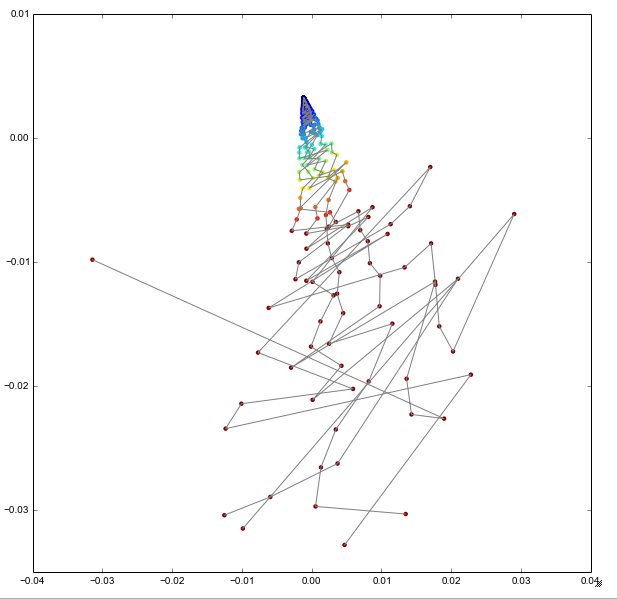
Figure 7: Simulated stochastic gradient descent of 5 random initial 1000-dimensional weight vector towards zero, after multidimensional scaling. At each time step, a dimension is chosen uniformly at random and multiplied by 0.9

Figure 8 shows a slight variation of this, using an optimization procedure very similar to the previous one. But instead of picking each dimension to be reduced at random, dimension $i$ of the parameter vector is chosen with probability $\frac{1}{i}$ (Zipf’s law). This process now replicates the behavior of SGD training of MLPs very well: initially, parameter vectors are wildly different, but they converge towards a common local minimum while still retaining a memory of their initial conditions over many training steps and many orders of magnitude of the objective function.

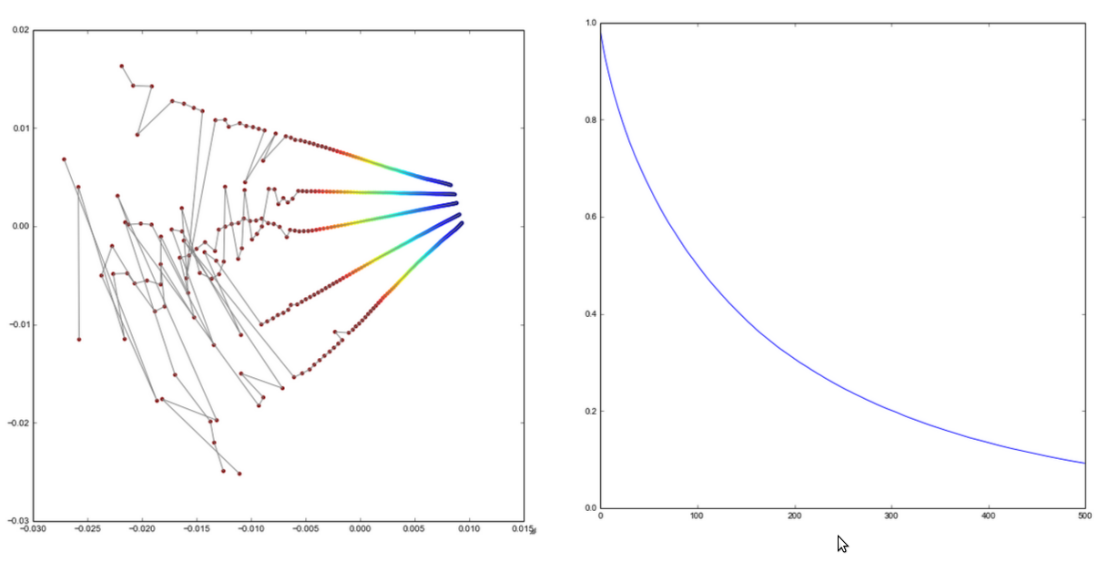
Figure 8: Simulated stochastic gradient descent of 5 random initial 1000-dimensional weight vector towards zero, after multidimensional scaling. At each time step, a dimension is chosen at random according to Zipf’s law and multiplied by 0.9

How does this simple stochastic model actually relate to MLP training? Notions of “local minima”, “valleys” and “basins of attraction” that are usually used to justify training strategies for MLPs really imagine the optimization problem to be one that makes complicated tradeoffs between many different parameters in the optimization of a single function. But we should actually think of the MLP training problem as that of optimizing a large collection of largely independent and unrelated functions. For example, the parameters that discriminate between the digits 4/9 are largely unrelated to the parameters that discriminate between the digits 0/8. Each such subtasks of the overall classification problem simply gets optimized at its own rate, depending on the frequency of relevant training examples. If training samples required for learning a particular subtask of the problem are rare, that subtask will converge slowly, while others converge fast.

4 Discussion and Conclusions

The experiments reported here suggest that the space in which SGD optimization of neural network weights takes place has properties that differ significantly from those usually assumed. In particular, the experiments show no evidence of the existence of local minima in which the optimization process gets trapped and they show no evidence of the existence of structures at different scales that would require decreasing the learning rate over time.

At the same time, these visualizations clearly show that networks retain “memory” of their initial random parameter initializations over hundreds of epochs and orders of magnitude of changes in outputs, weights, and error rates.

A tentative explanation of these observations is that SGD optimization of neural networks does not proceed as the optimization of a single function in a single space, but as an optimization of many functions in otherwise largely independent subspaces, where updates of different subspaces happen at greatly different rates. In the stochastic model used to illustrate this idea above, these independent subspaces were aligned with the coordinate axes, but they might also simply represent arbitrary linear or non-linear subspaces in weight space.

This view of weight space is somewhat related to ideas about optimization along “saddle points” that has been explored in second order learning methods for neural networks. However, if optimization really happens at very different rates in different subspaces, it points out another problem with second order methods: it means that the estimate of the local second order structure of the objective function in weight space will have very different variances in different directions.

Although these results seem generally consistent with training of other network architectures (provided they are sufficiently large) and training on other data sets, they remain to be verified. In particular, it is interesting to see how these results carry over to recurrent neural networks and LSTMs.

A model of SGD neural network optimization that views this optimization as optimization of largely independent subspaces at different rates has potential implications for the construction of better training algorithms; these will be explored in another paper.

References

- [1] Roberto Battiti. First-and second-order methods for learning: between steepest descent and newton’s method. Neural computation, 4(2):141–166, 1992.
- [2] Léon Bottou. Stochastic gradient learning in neural networks. Proceedings of Neuro-Nımes, 91(8), 1991.
- [3] Lars Kai Hansen and Peter Salamon. Neural network ensembles. IEEE Transactions on Pattern Analysis & Machine Intelligence, (10):993–1001, 1990.
- [4] Robert Hecht-Nielsen. Theory of the backpropagation neural network. In Neural Networks, 1989. IJCNN., International Joint Conference on, pages 593–605. IEEE, 1989.
- [5] Yann A LeCun, Léon Bottou, Genevieve B Orr, and Klaus-Robert Müller. Efficient backprop. In Neural networks: Tricks of the trade, pages 9–48. Springer, 2012.
- [6] Martin Riedmiller and I Rprop. Rprop-description and implementation details. 1994.
- [7] Nicol N Schraudolph. Local gain adaptation in stochastic gradient descent. In Artificial Neural Networks, 1999. ICANN 99. Ninth International Conference on (Conf. Publ. No. 470), volume 2, pages 569–574. IET, 1999.
- [8] Yi Shang and Benjamin W Wah. Global optimization for neural network training. Computer, 29(3):45–54, 1996.