The Mira-Titan Universe: Precision Predictions for Dark Energy Surveys

Abstract

Ground and space-based sky surveys enable powerful cosmological probes based on measurements of galaxy properties and the distribution of galaxies in the Universe. These probes include weak lensing, baryon acoustic oscillations, abundance of galaxy clusters, and redshift space distortions; they are essential to improving our knowledge of the nature of dark energy. On the theory and modeling front, large-scale simulations of cosmic structure formation play an important role in interpreting the observations and in the challenging task of extracting cosmological physics at the needed precision. These simulations must cover a parameter range beyond the standard six cosmological parameters and need to be run at high mass and force resolution. One key simulation-based task is the generation of accurate theoretical predictions for observables, via the method of emulation. Using a new sampling technique, we explore an 8-dimensional parameter space including massive neutrinos and a variable dark energy equation of state. We construct trial emulators using two surrogate models (the linear power spectrum and an approximate halo mass function). The new sampling method allows us to build precision emulators from just 26 cosmological models and to increase the emulator accuracy by adding new sets of simulations in a prescribed way. This allows emulator fidelity to be systematically improved as new observational data becomes available and higher accuracy is required. Finally, using one $\Lambda$CDM cosmology as an example, we study the demands imposed on a simulation campaign to achieve the required statistics and accuracy when building emulators for dark energy investigations.

1 Introduction

Cosmology has developed rapidly in the last few decades. The more qualitative original picture of the evolution of the Universe has evolved into a well-tested six-parameter “Standard Model of Cosmology”. Remarkably, this simple model describes all current observations at a level of accuracy of roughly a few percent, cementing a consistent picture of the Universe from a diverse set of cosmological probes. While this progress has truly revolutionized our knowledge of the Universe, a real understanding of its two main constituents, dark matter and dark energy, remains elusive.

To make progress towards solving these mysteries, as well as shedding light on other questions such as the sum of neutrino masses and the nature of primordial fluctuations, new ground- and space-based missions have been carried out (so-called Stage II experiments), are ongoing (Stage III), and are under construction or planned (Stage IV). These include the Baryon Oscillation Spectroscopic Survey (BOSS) (Schlegel, White, & Eisenstein, 2009), WiggleZ (Drinkwater et al., 2010), the Dark Energy Survey (DES), the Large Synoptic Survey Telescope (LSST) (Abell et al., 2009), the Dark Energy Spectroscopic Instrument (DESI), the Wide Field Infrared Survey Telescope (WFIRST) (Spergel, 2015), and Euclid (Refregier et al., 2010). The major science targets of these missions specific to dark energy are measurements of the large scale structure in the Universe on different scales (along with supernova distance measurements). Weak lensing, baryon acoustic oscillations (BAO), abundance of galaxy clusters, and redshift space distortions are the most prominent probes aimed at investigating the nature of dark energy. The upcoming surveys promise to obtain measurements of the main cosmology parameters at the 1% level accuracy if systematic errors can be sufficiently controlled.

To reach the desired accuracies, the physics of matter clustering on significantly nonlinear scales must be accurately modeled. Currently, the only way to do this is via expensive numerical simulations. Depending on the scales of interest and the required accuracy, different physical effects must be accounted for. On large scales relevant to, e.g., BAO, gravity-only simulations are likely sufficient for interpreting ongoing and upcoming measurements. For weak lensing, current surveys can be modeled with pure gravity simulations (see, e.g., the discussion in Heitmann et al. (2010)) but the interpretation of future surveys will require a treatment of baryonic effects (e.g., gas dynamics, feedback) and associated subgrid modeling.

Besides adding hydrodynamics effects and other modeling ingredients to the simulations, the cosmological parameter space has to be simultaneously widened. As argued in Heitmann et al. (2010), current observations do not have enough information to constrain cosmological parameters beyond $w$CDM scenarios – a mild extension of $\Lambda$CDM – at high accuracy. In the near future, however, it will be important to go beyond $w$CDM by including, e.g., dynamical dark energy models and at the same time accounting for “secondary” effects, currently too small to reliably extract from the measurements beyond setting upper or lower limits (such as a lower limit for $m_{\nu}$, the neutrino mass sum). The work here is aimed at a research program that covers the following eight-dimensional space: $p_{\theta}=\{\omega_{m},\omega_{b},\sigma_{8},h,n_{s},w_{0},w_{a},\omega_{\nu}\}.$ (Details are found in Section 2.)

1.1 Simulation Campaigns

If only a small number of simulations are required, the size of the parameter space is essentially irrelevant. This is, however, not the case in cosmology. Eventually one wishes to infer the values of the parameters from a set of observational measurements. Commonly used procedures for doing this all fall under the class of statistical inverse problems, where a large number of evaluations of the forward model (i.e., results from many simulations, at different specified parameter values) are necessary in order to use Markov chain Monte Carlo (MCMC) or other related methods. This may involve hundreds of thousands or even millions of forward model evaluations. (A similar issue is encountered in covariance estimation, where a large number of simulations are also needed.)

At first sight this problem may appear to be computationally overwhelming but it is in fact possible to cover large parameter spaces in an efficient manner with a drastically reduced number of simulations, provided certain smoothness conditions are met. The last requirement is largely satisfied in cosmological inverse problems, and this has allowed us to develop the “Cosmic Calibration Framework” (Heitmann et al., 2006; Habib et al., 2007; Heitmann et al., 2009; Lawrence et al., 2010; Higdon et al., 2010; Heitmann et al., 2014). The major components of the framework are:

• Sophisticated sampling methods that provide optimal coverage of the parameter space. In previous work we used a symmetric Latin hypercube design, as explained in Heitmann et al. (2009) (for a more technical presentation, see Santner et al. 2003). The new strategy presented here allows us to begin with a small set of cosmological models from which to construct a first set of emulators. These simulations are then systematically augmented to improve emulation accuracy. This defines a notion of strong convergence (Cf. Section 3) as opposed to the weak convergence previously demonstrated in Habib et al. (2007).

• High-dimensional interpolater based on Gaussian process modeling to build a prediction scheme (the emulator) for a diverse set of cosmological statistics of interest, e.g., the fluctuation power spectrum, the halo mass function, lensing statistics, etc.

• Emulator-based sensitivity analysis, characterizing the dependence of the cosmological statistics on different cosmological and modeling parameters.

• Final calibration step, which combines observational data and theoretical predictions to extract cosmological information from the data via MCMC methods.

We will focus on the first three steps and construct precision emulators for the power spectrum and the mass function; we also discuss extensions to other already existing emulators, e.g., for the concentration-mass relation (Kwan et al., 2013a) and the galaxy power spectrum and correlation function (Kwan et al., 2013b) below.

In this paper, we narrow our focus to work that directly impacts gravity-only simulations. The purpose here is to demonstrate the success of the basic methodology. Over time, we expect to include direct modeling of baryonic effects as well as indirect approaches based on post-processing gravity-only simulations. As has been mentioned previously, and discussed in several papers (White, 2004; Zhan & Knox, 2004; Jing et al., 2006; Rudd et al., 2008; van Daalen et al., 2011), deriving reliable predictions for cosmological statistics such as the power spectrum and the mass function eventually requires the treatment of gas physics, star formation, and feedback processes. As we explore smaller scales, these effects become more important. For the matter power spectrum, as an example, we expect effects at the 10-20% level at scales of $k\sim 10~{}h$Mpc^-1. Accounting for these effects via simulations poses two major difficulties: (i) the simulations are computationally very expensive, so only a limited number can be carried out; (ii) the physical models used in the simulations are too crude to be truly predictive; there is a rather large uncertainty in the modeling. Steady progress in this area is being made as hydrodynamical simulations become more affordable and understanding of the influence of baryonic physics improves. Examples of recent attempts to mitigate these uncertainties include the alteration of the halo concentration-mass relation and exploring how this change feeds back in, e.g., the power spectrum (Zentner et al., 2008). This approach can be explored within the halo model to obtain predictions for the power spectrum. More recently, it has been extended to include a range of hydrodynamic simulations and the calibration of how baryonic physics can bias the measurements from surveys like DES and LSST (Zentner et al., 2013). The idea is not to rely on carrying out a hydrodynamic simulation that is accurate in all its details, but rather to construct an approach that can mitigate uncertainties and biases due to baryonic effects in robust ways.

Finally, a major challenge is posed by the need for accurate predictions for covariances. The main difficulty here is the very large number of simulations that might be required to determine covariances at the accuracy needed as well as the uncertainties due to different cosmological inputs. Some early work in tackling these questions via emulation has been carried out by Schneider et al. (2008). Morrison & Schneider (2013) focus in particular on the question of cosmology dependence and emulation, basing their analysis on a halo model approach. As for baryonic effects, more work is required but first results are encouraging. We will not address either of these problems here but stress that our general emulation approach is directly applicable to these problems.

To attack the aforementioned challenges a multi-step comprehensive program has to be designed and carried out: (i) calibrate the underlying dark matter power spectrum and mass function for an 8-parameter model space out to $k\sim 5$Mpc^-1 and mass between $2\cdot 10^{12}$M_⊙ and $10^{15}$M_⊙ (at $z=0$, smaller cut-offs for high masses at higher redshifts) at high accuracy; (ii) extend the $k$-range to higher $k$ and mass range to lower masses by augmenting the simulation suite with a small number of simulations with very high mass resolution and use smart extrapolation approaches where applicable; (iii) add a small number of high-fidelity simulations including gas physics and re-calibrate the power spectra and mass functions for these effects; (iv) gauge the remaining uncertainties in the predictions and fold them into the calibration step.

Such a program is obviously very ambitious and will require significant effort and resources to be completed. In addition, community support and input are crucial – the simulation suite that will result from such a project can be used for a large number of scientific projects and has to be made available to the entire community. In order to accommodate as many follow-up projects as possible, it is important to have most analysis tools already in place and a comprehensive plan for post-processing so that the relevant data can be properly archived.

The goal of the current paper is to focus on the first step in some detail and demonstrate with surrogate models (such as the linear power spectrum and an estimated mass function) and a set of high resolution simulations that it is possible to successfully complete this program in accordance with the timelines of the major surveys. The paper will provide a roadmap that delivers prediction schemes at different levels of accuracy at different times – culminating finally in high-accuracy emulators that will be required for extracting the most science from surveys such as LSST. It introduces a new statistical approach for designing a simulation campaign that will lead to improved emulators over time. We also show results from simulations to investigate the optimal size of the simulations to be carried out, considering limited computational resources as well as accuracy requirements. We strongly believe that the community has to discuss and add to this roadmap to make such a project successful. Therefore, a paper outlining the plan and the solutions to the problem and showing that it is feasible before embarking on this endeavor is crucial.

The paper is organized as follows. In Section 2, we discuss the parameter ranges covered by our study and how we derived them. We then introduce a new design strategy for a simulation campaign that can be augmented over time and will lead to higher accuracy emulators with each new set of simulations (Section 3). A short overview on the N-body simulations that will be employed for the project is presented in Section 4. In the following sections, we focus on precision predictions for the dark matter power spectrum (Section 5) and the halo mass function (Section 6) using this new strategy. We present convergence studies and demonstrate that a set of $\sim$100 cosmological models suffice to reach the required accuracy. We also use a set of high resolution simulations to investigate the requirements for each individual model to mitigate uncertainties due to realization scatter. In Section 7 we summarize additional emulator projects that can be envisioned and conclude in Section 8 with a summary and short discussion.

2 Parameter Ranges

As discussed in the Introduction, a major challenge posed by upcoming surveys is the increase in parameter space that must be handled. In Heitmann et al. (2009), we discussed the requirements for ongoing weak lensing surveys and concluded that a five dimensional parameter space with $p_{\theta}=\{\omega_{m},\omega_{b},\sigma_{8},n_{s},w_{0}\}$ was sufficient to capture the information from contemporary measurements. In this scenario, we assume flatness, no running of the spectral index $n_{s}$, massless neutrinos, and constraints on the Hubble parameter $h$ from measurements of the distance to last scattering.

In this paper, we build upon the results obtained in Heitmann et al. (2009) and Planck constraints (Ade et al., 2013) and increase the parameter space by three additional parameters. We extend our previous analysis by letting $h$ be a free parameter, allow for a dynamical dark energy component via a two-dimensional parameterization $(w_{0},w_{a})$, and allow for massive neutrinos via $\omega_{\nu}$ but still keep the assumption of three relativistic species. For the first five parameters we keep the same parameter ranges as in Heitmann et al. (2009) and we refer the reader to that paper for more details on the reasoning behind our choices. We provide justifications for the chosen additional parameter ranges below. With the Planck data at hand, we keep the assumptions of flatness, $\Omega_{k}=0$, and no running of the spectral index, $d\log n_{s}/d\log k=0$. In summary, we investigate the following eight parameters within the ranges:

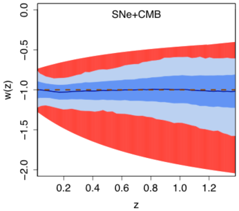
Figure 1: Constraints for the dark energy equation of state parameter $w(z)$ from supernova and CMB data in blue (light blue: 95% confidence level, dark blue: 68% confidence level, red dashed line: $w=-1$) from Holsclaw et al. (2011). The inclusion of baryon acoustic oscillations would tighten the constraints further. The red shaded region shows the range for $w(z)$ covered by our choices for $w_{0}$ and $w_{a}$ for our main design, comfortably including the best current constraints.

$$0.12\leq \omega_{m} \leq 0.155$$ (1)

$$0.0215\leq \omega_{b} \leq 0.0235$$ (2)

$$0.7\leq \sigma_{8} \leq 0.9$$ (3)

$$0.55\leq h \leq 0.85$$ (4)

$$0.85\leq n_{s} \leq 1.05$$ (5)

$$-1.3\leq w_{0} \leq-0.7$$ (6)

$$-1.5\leq w_{a} \leq 1.15$$ (7)

$$0.0\leq \omega_{\nu} \leq 0.01.$$ (8)

For these parameter ranges our aim is to obtain high precision predictions for different observables, at the percent level of accuracy.

Figure 2: Coverage of the $(w_{0},w_{a})$ plane. Red crosses show the design points with zero neutrino masses, green crosses the first 26 models, blue stars the next set of 29 models, and pink boxes the remaining 46 models. The upper dashed line shows the limit $w_{0}+w_{a}<0$ obeyed by all the models. The area shown approximately covers the constraints obtained from Planck data combined with the Union2.1 or SNLS supernova data set (see Fig. 36 in Ade et al. 2013). Models above the dotted line ($w_{0}+w_{a}=0$) are not considered.

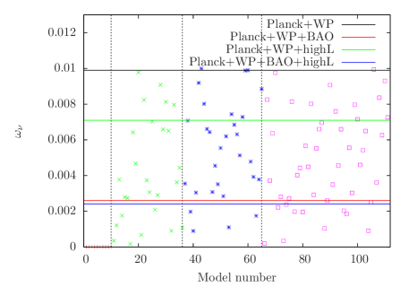
Figure 3: Current upper bounds on $\omega_{\nu}$ from Planck and combinations of different cosmological probes for a $\Lambda$CDM cosmology (values from Table 10 in Ade et al. 2013). WP stands for WMAP polarization data, the BAO measurements include several different surveys, the ‘highL’ CMB measurements are from the Atacama Cosmology Telescope and the South Pole Telescope. The red symbols show the values for $\omega_{\nu}$ in our design for the 101+10 models we consider throughout the paper. The first ten models have $\omega_{\nu}=0$ to provide good coverage of the current Standard Model. The symbols have the same meaning as in Fig. 2.

In Heitmann et al. (2009), we determined the best fit value for the Hubble parameter $h$ for each model from CMB measurements of the distance to last scattering. The power spectrum emulator (Lawrence et al., 2010) simply output the best fit value for any other emulated model. In the extended Coyote emulator (Heitmann et al. 2014) we provide the power spectrum prediction out to higher $k$- and $z$-values as well as treat the Hubble parameter as a free parameter in an approximate way. This extended emulator is based on the same cosmological models as the original emulator, which did not allow us to provide sub-percent accurate predictions including $h$ as a free parameter. Instead, we used results from higher order perturbation theory to follow the behavior of the power spectrum under changing $h$ (for sufficiently small values of $k$).

In the current paper, we keep $h$ as a free parameter embedded in the full design. We choose the range according to the minimum and maximum value we found in the model space in Heitmann et al. (2009). This range is rather large with respect to currently available constraints on $h$ – recent measurements shown in Riess et al. (2011) constrain $H_{0}$ at the 3% accuracy level to $73.8\pm 2.4$ km/s/Mpc, suggesting that measurements at the level of 1% accuracy are possible – but we want to ensure that the previously investigated parameter space is comfortably embedded in the new one. In addition, the rather low value for $H_{0}=67.3\pm 1.2$ km/s/Mpc found by the Planck team suggests that the error estimate in Riess et al. (2011) might be underestimated.

Next, we discuss our choices for the range of $w_{0}$ and $w_{a}$. The uncertainty in these parameters, in particular $w_{a}$, is still very large and reducing it is a major target of the upcoming surveys. We therefore allow a large range for both parameters, informed by constraints from supernova and CMB data. In Fig. 1 we show constraints obtained from a non-parametric reconstruction approach for $w(z)$ using recent supernova and CMB constraints (see Holsclaw et al. 2011 for details). The blue regions show the constraints at the 95% and 68% confidence level while red shaded region shows the coverage by our main models. Current constraints are therefore comfortably covered by our allowed parameter ranges. A similar view, but this time aimed at current parametric constraints on $(w_{0},w_{a})$ is shown in Fig. 2. Here we show the coverage of the $(w_{0},w_{a})$ parameter plane and scale the axis approximately following Fig. 36 in Ade et al. (2013) which provides constraints from CMB and supernova measurements. Again, with the ranges as chosen, we provide good coverage of the currently favored regions of parameter space.

Finally, our choice for the range on the neutrino mass parameter $\omega_{\nu}$ is informed by the constraints available from the Planck measurements. In Fig. 3 we show different limits given by Planck in combination with other surveys. Note that these limits were derived for $\Lambda$CDM models. For our broader model space they would be less stringent. We therefore choose to follow the most conservative bound (Planck + WP). The WMAP team has considered neutrino mass bounds for $w$CDM models and even for those our chosen parameter range comfortably covers all currently allowed mass values.

3 Design Strategy

An important challenge for building efficient emulators in the nonlinear regime is overcoming the high cost of accurate simulations. It is not possible to evaluate the simulator over and over in a brute force fashion. Given this hard constraint, a judicious choice of simulation design (i.e., the simulation suite of models) is essential. For us, this means varying the eight parameters over the ranges specified in Eqns. 1 so that the parameter space is optimally sampled.

The emulation strategy relies heavily on Gaussian process (GP) models (see, e.g., Sacks et al. 1989; Rasmussen & Williams 2006) to interpolate across the simulation results. Johnson et al. (1990) showed that under certain conditions, designs with good space-filling properties (e.g., maximizing the minimum distance between the design points - maximin designs) are optimal for GPs. This is because a prediction from a GP emulator is a weighted average of the data inputs (simulation inputs in our case), where the outputs from nearby models have higher weights than those far from the prediction location.

A very important new feature with our simulation design is that we aim to progressively fill the model space so that intermediate analyses can be performed while the remaining simulations continue to run. Hence, a simulation design is required that simultaneously combines (i) good space-filling properties for the chosen number of sampling points and (ii) also provides good space-filling properties at intermediate stages of the sampling process. Together (i) and (ii) ensure that the final and intermediate stage simulation designs give good coverage of the model space so that efficient emulators can be constructed in a staged, convergent fashion. To achieve this goal, we use a space-filling design based on point lattices.

It is worth noting that Latin hypercube designs (McKay et al., 1979) are frequently used in simulation based “experiments”, as in our previous work. These designs impose one-dimensional space-filling. To make them better suited to computer model emulation with GPs, additional space-filling criteria, e.g., maximin Latin hypercube designs (Morris & Mitchell 1995), are imposed to improve the design. The nested lattice scheme we use here has the added benefit of explicitly enforcing space-filling properties in intermediate stages of the simulation campaign as well as in the final design.

3.1 Space-filling lattice designs

A point lattice $\Lambda$ is an infinite set of points in $\mathbb{R}^{d}$ constructed as integer multiples of a set of basis vectors that are given as columns of a non-singular generating matrix $\;\mathbf{G}\in\mathbb{R}^{d\times d}$

$$\Lambda(\mathbf{G})=\{\mathbf{G}\mathbf{k}:\mathbf{k}\in\mathbb{Z}^{d}\}\subset\mathbb{R}^{d},$$ (9)

writing $\Lambda(\mathbf{G})$ instead of $\Lambda$ only when the generating matrix is needed to differentiate between lattices. The familiar Cartesian lattice, for example, has the $d$-dimensional identity matrix as its generating matrix.

Since a lattice $\Lambda$ is a linear transformation of the integers $\mathbb{Z}^{d}$, $\Lambda$ inherits the integer’s Abelian group structure, i.e., for any point $\mathbf{x}\in\Lambda$ we have $\mathbf{x}+\Lambda=\Lambda$. A Voronoi cell is the neighbourhood of points in $\mathbb{R}^{d}$ that are closer to a particular point $\mathbf{x}\in\Lambda$ than to any other point in $\Lambda$. Due to the translation invariance of $\Lambda$, its Voronoi cells look exactly the same for any $\mathbf{x}\in\Lambda$. Hence, a lattice basis $\mathbf{G}$ that is chosen to give a large packing sphere diameter among nearest neighbours (maximin distance) or small covering diameter (minimax distance) immediately imposes useful space-filling properties for the entire design region $\mathcal{M}$ as illustrated in Figure 4 (Conway & Sloane 1999; Johnson et al. 1990). It is traditional to scale all input parameters to the unit interval $[0,1]$ to put all parameters on the same footing in the analysis. Thus, it is convenient to write the input region as the $d$-dimensional unit cube $\mathcal{M}=[0,1]^{d}$ with volume $\text{vol}(\mathcal{M})=1$.

A lattice design is the intersection of the lattice and the design region (or input region) of interest, possibly shifted to achieve useful statistical properties. More formally, $X=\mathcal{M}\cap\Lambda+\mathbf{p}$ for input region $\mathcal{M}$ is obtained by restricting the infinite lattice to the region with a possible shift of $\Lambda$ by some $\mathbf{p}\in\mathbb{R}^{d}$. A straightforward approach for finding a lattice design is given in Algorithm 1.

Algorithm 1 A method to produce a lattice design $X(\mathcal{M},\mathbf{G},\mathbf{p})$ in the region $\mathcal{M}=[0,1]^{d}$ for any generating matrix $\mathbf{G}$ and shift of origin $\mathbf{p}$.

1. Determine a finite candidate subset of lattice point indices $K^{\prime}\subset\mathbb{Z}^{d}$ that produce all design points that are potentially contained in $[0,1]^{d}$.
   For instance, enumerate all integer points in the axis-aligned bounding box that contains the inverse image $C^{\prime}$ of all corners of the design region $\mathcal{M}$, $C^{\prime}=\left\{\mathbf{G}^{-1}(\mathbf{c}-\mathbf{p}):\mathbf{c}\in\{0,1\}^{d}\right\}$. With lower bound $\mathbf{l}\in\mathbb{Z}^{d}$ that is constructed as $l_{i}=\lfloor\min\{k_{i}:\mathbf{k}\in C^{\prime}\}\rfloor$ and analogous upper bound $\mathbf{u}\in\mathbb{Z}^{d}$, the candidate indices are $K^{\prime}=\{l_{1},l_{1}+1,\dotsc,u_{1}\}\times\{l_{2},l_{2}+1,\dotsc,u_{2}\}\times\dots\times\{l_{d},l_{d}+1,\dotsc,u_{d}\}$.

2. Produce a superset of the design as $X^{\prime}=\left\{\mathbf{G}\mathbf{k}+\mathbf{p}:\mathbf{k}\in K^{\prime}\right\}$.

3. Keep all points from $X^{\prime}$ with coordinates $0\leq x_{i,j}\leq 1$ to obtain the design $X$.

Note, to be able to produce lattice designs for larger $d$ it is essential to improve the construction of $K^{\prime}$ in step 1. To sketch the approach here, start by covering a one-dimensional projection of $\mathbf{G}^{-1}(\mathcal{M}-\mathbf{p})$ to build the design iteratively, adding one dimension at a time.

3.2 Searching for a good lattice design

The choice of $\mathbf{G}$ and $\mathbf{p}$ in Algorithm 1 leaves only $d^{2}+d$ degrees of freedom in optimizing further useful experimental design criteria. This is important to finding good designs for large dimensionality $d$ and simulation experiment runsizes $n=\left|X\right|$, because without the lattice constraint this would be a $d\cdot n$-dimensional, non-convex optimization problem. Furthermore, known constructions for good generating matrices $\mathbf{G}$ are readily available (Conway & Sloane 1999), leaving only a suitable rotation $\mathbf{Q}\in\mathrm{SO}(d)$ to produce alternative bases $\mathbf{Q}\mathbf{G}$.

When a lattice is shifted or rotated, design points can move in and out of the fixed design region $\mathcal{M}$. The expected runsize, $\hat{n}$, of a randomly rotated and shifted lattice within the unit cube $\mathcal{M}$ is $\hat{n}(\mathbf{G})=\mathrm{E}\left[\left|X(\mathcal{M},\mathbf{Q}\mathbf{G},\mathbf{p})\right|\;:\;\mathbf{p}\in\mathbb{R}^{d},\mathbf{Q}^{T}\mathbf{Q}=\mathbf{I}\right]=1/\left|\det\mathbf{G}\right|$. To achieve a certain desired runsize $N$, at least in expectation, we scale $\mathbf{G}$ such that $\det\mathbf{G}=1/N$, before performing Algorithm 2.

Algorithm 2 A method to find a shift $\mathbf{p}$ and initial rotation $\mathbf{Q}_{0}$ of a lattice $\Lambda$ that produce a design with a desired runsize $N=1/\det\mathbf{G}$ and other possible design criteria.

1. Start with an empty set of known designs $\mathcal{K}$.

2. Do the following for a certain number of trials (batch size).

   1. Choose a random shift $\mathbf{p}\in\mathcal{M}$ and produce a random rotation $\mathbf{Q}$ via QR-decomposition of a random matrix.

   2. Generate the lattice design $X(\mathcal{M},\mathbf{Q}\mathbf{G},\mathbf{p})$ via Algorithm 1.

   3. Calculate all design performance criteria $c_{l}(X)$ and store them as assessment $\mathbf{c}$. This may just include the desired runsize $N$ criterion $c_{\text{runsize}}=\left|(\left|X\right|-N)\right|$. If $\left\|\mathbf{c}\right\|=0$, terminate the search and return design $X$ with rotation $\mathbf{Q}_{0}$ and $\mathbf{p}$.

   4. Add the tuple $(\mathbf{Q},\mathbf{p},\mathbf{c})$ to the current batch of trial designs.

3. Add the current batch of designs to the set of known designs $\mathcal{K}$.
   Repeat step 2, if the assessments $\mathbf{c}$ of known designs $\mathcal{K}$ have changed significantly, for instance, as determined by the $\mathcal{L}_{1}$ distance of the percentile functions of empirical distributions of $\left\|\mathbf{c}\right\|$ in $\mathcal{K}$ vs. $\mathcal{K}$ joined with the current update batch of trials.

4. Return one of the best known designs, i. e. by choosing one with the smallest $\left\|\mathbf{c}\right\|$.

3.3 Sequences of nested lattice designs

A further desirable property of a sequence of design points is that they approach a uniform distribution — ideally ensuring good coverage for prediction at earlier run sizes. This means, for example, that even with a potential simulation budget of $200$ simulation runs, the first $25$ could be chosen so that they can inform a decision as to whether resources should be allocated to compute a further $25$ runs, then $50$, and then another $100$ experimental points to gain further insight.

In this section, we show how to obtain a sequence of lattice designs that progressively fills the parameter (input) space. First, observe that a sequence of nested lattices is a hierarchy of lattices. To decompose a fine lattice $\Lambda(\mathbf{G})$ into coarser lattices, the generating matrix changes into $\mathbf{G}\mathbf{K}$ for dilation matrix $\mathbf{K}$. Central to the construction of nested lattice designs is that $\Lambda(\mathbf{G}_{0})\supset\Lambda(\mathbf{G}_{1})\Leftrightarrow\mathbf{G}_{0}^{-1}\mathbf{G}_{1}=\mathbf{K}\in\mathbb{Z}^{d\times d}$. In other words, any sequence of nested lattices

$$\dotsc\supset\Lambda(\mathbf{G}_{0})\supset\Lambda(\mathbf{G}_{1})\supset\dotsc$$ (10)

is equivalent to a sequence of dilation matrices $\mathbf{K}_{l}$ being integer, where $\mathbf{G}_{l+1}=\mathbf{G}_{l}\mathbf{K}_{l}$. The initial lattice $\Lambda(\mathbf{G}_{0})$ itself, however, does not have to be a subset of the integers.

The expected runsize $\hat{n}$ or density of $\Lambda(\mathbf{G})$ is increased by a factor of $\left|\det\mathbf{K}\right|=\beta\in\mathbb{Z}$ as opposed to the coarser sub-lattice $\Lambda(\mathbf{G}\mathbf{K})$. It is possible to choose the factor $\beta$ as low as two. So, we can construct a sequence of lattice designs with expected run-sizes that change by a factor of two.

Here we provide a new method for constructing a sequence of nested lattice designs. This is achieved by developing a construction for a single dilation matrix, $\mathbf{K}$, so that $\mathbf{K}^{-1}$ can be used many times to obtain refined designs that yield large run sizes $n$. That is, we start with a coarse lattice, and apply the inverted dilation matrix, to get larger designs. The larger lattice designs contain the smaller lattice designs and thus have good space-filling properties at intermediate run sizes if performed in a sequence.

More precisely, our construction is giving all non-equivalent integer matrices $\mathbf{K}$ that give a sequence of lattices

$$\dotsc\supset\Lambda(\mathbf{G}\mathbf{K}^{-1})\supset\Lambda(\mathbf{G})\supset\Lambda(\mathbf{G}\mathbf{K})\supset\dotsc$$

that also have a rotational symmetry

$$\mathbf{Q}\mathbf{G}=\mathbf{\mathbf{G}}\mathbf{K}$$ (11)

for a uniformly $\alpha$-scaled rotation matrix $\mathbf{Q}$ that fulfills $\mathbf{Q}^{T}\mathbf{Q}=\alpha^{2}\mathbf{I}$ with $\alpha^{d}=\det\mathbf{Q}=\det\mathbf{K}$.

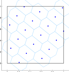
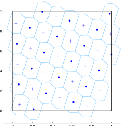
Figure 4: The 19 point set (a) is a subset of the 37 point refined design (b), which is a rotated version of (a) that has twice the density of sample points.

Equation 11 suggests an equivalent viewpoint to our construction — the sequence of nested designs is constructed from uniformly scaled rotations $\mathbf{Q}$ of a specific initial lattice $\Lambda(\mathbf{G})$. To find a suitable initialization $X$ for the design sequence, the generating matrix $\mathbf{G}$ can be scaled and rotated to optimize some criteria using Algorithm 2. Coarser sub-designs $X_{l}$ based on $\Lambda(\mathbf{Q}^{l}\mathbf{G})$ or equivalently $\Lambda(\mathbf{G}\mathbf{K}^{l})$ for $l=1,2,\dotsc$, as well as refined designs for negative $l$ can be obtained via Algorithm 1.

A hierarchical ordering of points is obtained by decomposing $X$ and by running the points in $X_{l}$ without repetition in decreasing order starting with the largest $l$. In practice, the $l^{\text{th}}$ sub-grid $X_{l}$ is determined by retaining all points of $\{\mathbf{K}^{-l}\mathbf{k}:\mathbf{k}\in\mathbf{G}^{-1}(\mathbf{x}-\mathbf{p}):\mathbf{x}\in X\}$ that have integer coordinates only. A one-dimensional example $X_{1}$ with $\mathbf{K}=2$ are the even numbers formed from integer numbers that after a multiplication by $\mathbf{K}^{-1}$ are still integer.

The other key property of our construction is the nesting of the sequence of lattices

$$\Lambda(\mathbf{G})\supset\Lambda(\mathbf{Q}^{s}\mathbf{G})=\Lambda_{s}\text{for any scale }s=1,2,3\ldots.$$ (12)

The subset relationship in this sequence is the other way around if negative $s$ are used to produce a lattice refinement rather than coarsening. This means that we can start with a refined lattice and sub-sample using the matrix $\mathbf{Q}$. Or equivalently, we can start with a coarse lattice and refine it by applying the matrix $\mathbf{Q}^{-1}$ to the lattice basis to obtain a refined lattice. We can apply this matrix repeatedly to obtain coarser or, conversely, more refined lattices.

The choice of generating matrix $\mathbf{G}$ and rotation-scale matrix $\mathbf{Q}$ (Eqn. 11) to produce a nested design sequence are not independent. Bergner (2011) demonstrated that, given $d$ and sub-sampling rate $\beta=\det\mathbf{K}$, there are a limited number of integer matrices $\mathbf{K}$ with corresponding rotation-scale matrices, $\mathbf{Q}$, and $\mathbf{G}$, that can be considered — only four possibilities, $\mathbf{K}$ and $\mathbf{K}^{T}$ with possible scaling by $-1$, exist in case of odd $d$ and prime $\beta$.

The lattices obtained in this manner have good space-filling properties that lead to efficient prediction for GPs. In addition, the sequences from one coarse lattice to increasingly refined lattices of the same type gives very predictable improvement for the space filling properties (see illustration below).

Furthermore, unlike the Cartesian lattice where the size of the simulation suite grows exponentially with $d$, the non-rectangular lattices we use can achieve virtually any run-size. Perfect ratios $\beta$ among runsizes $|X_{l}|$ are not guaranteed, because some of the points in the refined design can lie outside of $\mathcal{M}$. To see this, we note that that the density of the lattice indicates the expected number of points per unit volume. An exact count in the most coarse designs is possible to achieve. However, we can find only a sequence of lattices where the expected number of design points is the desired size of the simulation design, and it is possible that a few additional points may enter $\mathcal{M}$ or have to be discarded. With Algorithm 2 it is possible in step (2c) to simultaneously match runsizes on multiple levels of coarsening $l$, as additional criteria $c_{l}$.

As an illustration, consider the 2-d example in Figure 4. Optimal choices of $\mathbf{Q}$ and $\mathbf{G}$ are found using the method described in Bergner (2011). A coarse design of $19$ points is found in Figure 4(a). The model runs represented by these points would be the first to perform in the simulation and become available for intermediate data analysis. The lattice is refined by adding another $18$ points (the number of simulations is almost doubled, but one of the design points in the refined lattice fell outside of $[0,1]^{d}$). This is done by applying the inverse of a dilation matrix to the coarse lattice (alternatively, the dilation matrix could be applied to the more dense lattice to obtain the coarse lattice). The combined design is shown in Figure 4(b). Notice that both the initial lattice and the refined lattice are rotated and scaled versions of the same lattice. Furthermore, the shape of the Voronoi regions are the same, and the volume of the refined cells (area in 2-$d$) is one-half the volume of the coarse cells.

The designs that we performed in the 8-dimensional input region above were constructed in exactly the same manner. That is, an initial lattice design was found for a run size of $n_{1}=25$. The next $n_{2}=27$ points were found by applying the inverse of a dilation matrix to the lattice and using the points that intersection the 8-dimensional unit hypercube. Finally, the last $n_{3}=47$ points were found in exactly the same way.

To summarize, space-filling design sequences can be obtained by extending a good initial lattice design to a coarsening or refining sequence of lattices. The rotational symmetry of the sequences developed here ensures directionally uniform density at each level of refinement.

3.4 Cosmological Considerations

Currently, observational constraints on neutrino masses are only upper bounds, and in the Standard Model of Cosmology we still have $m_{\nu}=0$. From a design stand-point, this puts the currently best-fit value for one of our parameters at the edge of the design (since centering the neutrino mass range around zero is excluded). In general, the accuracy of the emulator predictions start to degrade when they approach a design edge, due to lack of nearby points. In order to mitigate this problem, we add a set of 10 simulations with $m_{\nu}=0$ to the design. We choose the values for the remaining 7 parameters according to a symmetric latin hypercube design.

While checking the accuracy properties of a first test emulator, we noticed that models with $w_{0}+w_{a}$ approaching zero were not predicted very well. This was due to the fact that the behavior of these models on large scales is different compared to models closer to the Standard Model. With the other six parameters fixed, the correlation between two models with $w_{0}+w_{a}$ close to zero is lower than between two models with $w_{0}+w_{a}$ far from zero. Observationally, $w_{0}+w_{a}$ close to zero is already disfavored and predictions in this regime do not necessarily need to be accurate at the percent level. Nevertheless we aim to provide reliable predictions over the full parameter range we cover. Rather than alter our emulation scheme, we introduce a transformation of these two parameters to scale the distances in these parameters in a way that produces stationary behavior. After some exploratory data analysis, we replaced $(w_{0},w_{a})$ in the design space with $(w_{0},[-w_{0}-w_{a}]^{1/4})$. This transformation results in the desired behavior. This special treatment of $(w_{0},w_{a})$ pairs can be seen in Figure 2 – the design provides slightly more points close to the limit $w_{0}+w_{a}=0$.

4 $N$-body Simulations

The parameter range outlined in Section 2 requires some extensions of the standard setup for $w$CDM N-body simulations. In particular, dynamical dark energy models defined by an equation of state parametrized by $(w_{0},w_{a})$ have to be included as well as a treatment of massive neutrinos. In the following we will give a brief description of our implementations of these additions in the $N$-body code HACC (Hardware/Hybrid Accelerated Cosmology Code) described in detail in Habib et al. (2016).

In order to estimate the overall computational needs with regard to box size, mass and force resolution, number of realizations, and other considerations, we will also discuss results from a $\Lambda$CDM simulation suite throughout the following sections. We give a brief overview of the simulations here.

4.1 Required Modifications in the $N$-body Code

The modifications in the HACC code to include neutrinos and dynamical dark energy models are straightforward and have been discussed in Upadhye et al. (2014). In that work, HACC simulations were used to test the range of validity of the TimeRG (“Renormalization Group”) perturbation theory approach, introduced by Pietroni (2008) and Lesgourgues et al. (2009), focusing on massive neutrinos and dynamical dark energy models. This work will be an important ingredient for our planned power spectrum emulator development. We summarize the main points here and remind the reader of the approximate treatment of massive neutrinos that we employ. The impact of dynamical dark energy and neutrinos are taken into account by (i) modifying the initializer and (ii) including both effects in the background evolution.

4.1.1 Neutrinos

Simulating neutrinos fully self-consistently as a separate particle species in a cosmological simulation is nontrivial mainly due to two reasons: (i) the very large neutrino velocities at early times due to the thermal velocity contribution which make very small time steps necessary, (ii) the large mass difference between the tracer particles representing dark matter and neutrinos respectively, which can lead to scattering artifacts if not treated properly. Over the years, many different solutions have been suggested to overcome these problems, from starting the (neutrino) simulation very late (leading to a different set of problems and inaccuracies) to simulating the neutrinos on a coarser grid to treating the neutrinos only linearly. An incomplete list of papers employing different solutions include Klypin et al. (1993), Gardini et al. (1999), Brandbyge et al. (2008), Brandbyge & Hannestad (2009), Brandbyge & Hannestad (2010), Viel et al. (2010), Bird et al. (2012), and Agarwal & Feldman (2011).

In our work, we follow closely the approach used in Agarwal & Feldman (2011) with some modifications. We do not include the nonlinear evolution of the neutrinos but instead evolve the cold dark matter-baryon component ($cb$) only, including the neutrinos in the background evolution. In order to obtain the total matter power spectrum, we add at any given output the linear component of the neutrino power spectrum to the nonlinear $cb$ matter power spectrum in the following way:

$$P_{total}^{nl}(k,a)=\left[\sqrt{P_{cb}^{nl}(k,a)}+\sqrt{P_{\nu}^{lin}(k,a)}\right]^{2}.$$ (13)

This treatment is justified since neutrinos are massive enough to behave matter-like close to $z=0$ but light enough to not cluster strongly on small scales. In Upadhye et al. (2014) we investigated the validity of this approximation on large to quasi-nonlinear scales and found sufficiently small errors for neutrino masses below the currently excluded value.

When setting the initial conditions, we include the neutrino contributions in the transfer function and generate a linear power spectrum at $z=0$ normalized to a given $\sigma_{8}$. Then, the $cb$ component of the matter power spectrum is moved back to the initial redshift with a scale-independent growth function (the growth function that includes neutrinos would be scale-dependent). This growth function includes all the species in the homogenous background. Note that using a scale-dependent growth function would be inconsistent since the evolution to $z=0$ is carried out for the $cb$ component. The setup described here ensures that at $z=0$ the power spectrum matches the full linear power spectrum on large scales. Finally, in the evolution the massive neutrinos are included in the background evolution equation, but we do not source the neutrino growth in the Poisson equation. For a detailed discussion of the implementation as well as various tests, the reader is referred to Upadhye et al. (2014).

4.1.2 Dynamical Dark Energy Equation of State

Next, we discuss our treatment of a dynamical dark energy equation of state. Without a compelling theory for a dark energy model beyond the cosmological constant, the simplest way to express a dynamical origin for dark energy is to parameterize the dark energy equation of state $w(z)$ via a time varying functional form described by two parameters ($w_{0},w_{a}$). A commonly used form is that suggested by Chevalier & Polarski (2001) and Linder (2003):

$$w(a)=w_{0}+w_{a}(1-a).$$ (14)

In order to account for the time dependent dark energy equation of state in the initial conditions of the simulations, we need to generate a transfer function that includes the effects from $w(z)$. For this, we modify the publicly available version of CAMB (Lewis et al., 2000) and include the dynamical dark energy in the evolution of the background as well as modify the equations describing the density and velocity perturbations in the dark energy.

To modify the background cosmology, we simply have to change the equation describing the evolution of conformal time as a function of the scale factor. Modifying the equations describing the perturbations of dark energy requires an expression for the speed of sound. In analogy with a simple scalar field model, we assume that this is the speed of light. As a result, perturbations of dark energy develop only on the Hubble scale. A second issue is that the equations describing the evolution of the velocity perturbations include terms of the form $c_{s}^{2}/(1+w(a))$, where $c_{s}$ is the speed of sound in the rest frame of dark energy. For those values of $(w_{0},w_{a})$ for which the equation of state passes through $-1$, this results in a singularity. We treat this by assuming the microscopic properties of dark energy do not modify the power spectra, and so this term is small when $w(a)$ crosses $-1$. Next, we need to include $(w_{0},w_{a})$ in the growth function in order to set up the initial conditions at the desired redshift. This is achieved by evaluating the integral over $w(a)$ that appears in $H^{2}(a)$ in the growth function: $-3\int^{a}_{1}da^{\prime}[w(a^{\prime})/a^{\prime}]=a^{-3(w_{0}+w_{a})}\exp[-3w_{a}(1-a)]$. Finally, the modifications in the Vlasov-Poisson equation for the time evolution to include $(w_{0},w_{a})$ are also simple. In the case of HACC, the expansion factor $a$ is used as the time variable, and therefore the only change again is in $H(z)$ and the corresponding scale factor expressions.

4.2 $\Lambda$CDM Simulation

In order to test our overall simulation strategy with regard to resolution and sufficient statistics, we carry out two high-resolution $\Lambda$CDM simulations. These simulations represent the specification of the main simulation suite that will be carried out for each model in our future work. In addition to these high mass and force resolution simulations, we will augment each model with a set of lower resolution simulations to cover the full dynamic range with sufficient accuracy as required. The cosmological parameters are chosen to be close to the best-fit WMAP-7 parameters (Komatsu et al. 2011): $\omega_{m}=0.1335,~{}\omega_{b}=0.02258,~{}n_{s}=0.963~{},w=-1.0,~{}\sigma_{8}=0.8~{},h=0.71$. In one simulation we evolve 3200³ particles in a (2100 Mpc)³ volume, leading to a mass resolution of $m_{p}\sim 10^{10}$M_⊙. The force resolution is chosen to be $\sim$6.6 kpc. This simulation has been previously used to validate the accuracy of a $w$CDM power spectrum emulator (Heitmann et al., 2014) and to create an emulator for the galaxy power spectrum (Kwan et al., 2013a) based on halo occupation distribution (HOD) modeling. The idea behind using an HOD to generate galaxy catalogs is straightforward (Kauffmann et al. 1997; Jing et al. 1998; Benson et al. 2000; Peacock & Smith 2000; Seljak 2000; Berlind & Weinberg 2002; Zheng et al. 2005). The HOD provides a prescription for the galaxy population (central and satellites) for a halo as a function of halo mass. The HOD parameters are obtained from matching the resulting galaxy correlation function to observations. For different types of galaxies, the HOD will be specified by different parameter values. The resolution of our simulations is sufficient for a wide range of investigations and to build detailed synthetic skies in different wavebands.

The specifications of the additional simulations needed to generate accurate emulators depend on the statistics of interest. As we show below, for the power spectrum predictions we require a set of particle-mesh (PM) runs for the quasi-linear regime to suppress the noise due to realization scatter. For the mass function, we require large volume simulations with high force resolution in addition to the simulation described above to cover the cluster mass range. As we show in Section 6, a simulation covering a volume of (5600 Mpc)³ evolving 4096³ particles is optimal for this purpose. Due to the modest mass resolution of $\sim 10^{11}$M_⊙ and – as we show below – the rather small number of time steps needed to achieve sufficient accuracy, the cost of these large simulations is reasonable. A summary of the $\Lambda$CDM simulations used in this paper is given in Table 1.

Table 1: Simulation specifications

$n_{p}$	$L$[Mpc]	Realizations	Force resolution [kpc]
32003	2100	1	6.6 (high-res)
40963	5634	1	13.8 (high-res)
5123	1300	16	1270 (PM)

5 The Power Spectrum

5.1 Smooth Power Spectrum Predictions

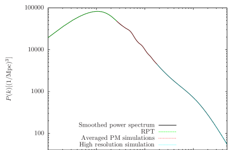
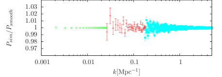
Figure 5: Upper panel: Power spectrum at $z=0$ assembled from RPT (green dashed), the average of 16 PM simulations (red dashed), and one high resolution simulation at large scales (light blue dotted). The black curve underneath the simulation/perturbation theory results shows the smooth power spectrum extracted from this ensemble. In order to demonstrate the quality of the smoothing procedure, we show the ratio of these results in the lower panel, including error bars calculated from the finite number of modes at each bin for the simulation results.

Following the discussions in Lawrence et al. (2010) and Heitmann et al. (2014), a major obstacle in extracting a smooth power spectrum from a simulation campaign is due to realization scatter. In order to solve this problem, we have shown that a smoothed power spectrum can be achieved by matching higher order perturbation theory on the largest scales with medium resolution, particle mesh (PM) runs (many realizations) on intermediate scales, and a high resolution simulation on small scales. In addition to this matching procedure, we have developed a sophisticated smoothing method based on a process convolution approach described in Higdon (2002). The main idea behind this approach is to build a smooth function as a moving average of a simple stochastic process. The moving average uses a smoothing kernel with a varying width – in regions with distinct features like the baryon acoustic oscillations the window is narrow while in very smooth regions such the very small scales, the window can be wider. We will use the same method again here. We cover a $k$ range between 0.001 to 6 Mpc^-1 via matching (i) renormalized perturbation theory out to $k\sim 0.04$ Mpc^-1 for $z=0,~{}1$ and $k\sim 0.14$ Mpc^-1 for $z=2$; (ii) 16 realizations of PM simulations with 512³ particles on a 1024³ grid in a (1300 Mpc)³ volume out to $k\sim 0.25$ Mpc^-1; (iii) a (2100Mpc)³ volume, high-resolution simulation with 3200³ particles and 6.6 kpc force resolution to cover the remaining $k$-range.

Figure 5 demonstrates the matching and smoothing strategy for our fiducial $\Lambda$CDM model, M000, described in Section 4.2. The power spectrum was obtained from the simulation in the same way as described in Heitmann et al. (2010) via mapping the particles onto a large grid (6400³ in this case) using a cloud-in-cell (CIC) assignment, applying an FFT, correcting for the charge-assignment window function and averaging the results in bins in $|{\bf k}|$. We show results for both $P(k)$ and the dimensionless power spectrum $\Delta^{2}(k)$, connected via the following relation:

$$\Delta^{2}(k)=\frac{k^{3}P(k)}{2\pi^{2}}.$$ (15)

We only present results at $z=0$ here, for $z=1$ and $z=2$ the reader is referred to the Appendix of Heitmann et al. (2014). The upper panel shows the full power spectrum assembled from RPT, PM simulations, and one high-resolution run on top of the smoothed power spectrum. On the logarithmic scales used here, even without the smoothing, the result is already very good. The lower panel shows the ratio of the smoothed power spectrum to the simulations; the aim of this figure is to demonstrate that the matching does not lead to any bias. These results show that our matching and smoothing strategy works as desired. We also point out that the large simulation volume paired with good mass resolution allows us to push out to higher $k$ without having to rely on small simulation volumes, which can induce some inaccuracy, as was shown in  Heitmann et al. (2014).

5.2 Emulator Performance

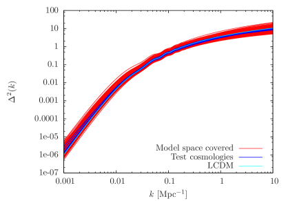
Figure 6: Power spectrum model space covered by 101 cosmological models within the range described in Eqs. (1), shown in red. Test models are shown in blue, where the light blue curve shows M000, a $\Lambda$CDM model, and the dark blue curves show the additional models specified in Table 2.

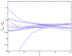
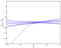
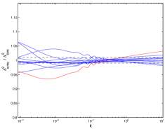
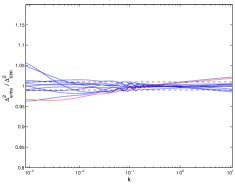
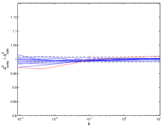
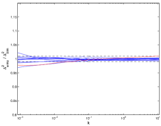
Figure 7: Emulator test: An emulator for the linear power spectrum is tested using 10 reference cosmological models. The emulator predictions built from up to 101 models are compared to the exact linear spectra from CAMB in the left panels and predictions from up to 111 models in the right panels. Shown is the ratio of prediction to “truth”, the emulator predictions are accurate at the 1% level (dashed line) on small scales. The upper panels shows the prediction for an emulator based on 26/36 models, the middle panel is based on 55/65 models, and for the predictions shown in the lower panel all 101/111 models were used. The red line shows the prediction accuracy for a $\Lambda$CDM model.

Following the strategy outlined in Section 3 we now discuss the accuracy we expect to achieve from 101 simulation models, obtained in a three-step simulation campaign. The first set of power spectra covers 26 models, the second set 55, and the final set covers all 101 models. In addition, as discussed in Section 3 we add 10 models with $m_{\nu}=0$ to properly cover this important edge of the design hypercube.

For our tests, we use linear power spectrum predictions generated with CAMB. This allows us to obtain many power spectra with nominal computational effort. At the same time, the linear power spectrum has been proven to be a very good testbed for the final nonlinear emulator (see, e.g., Heitmann et al. 2009). Figure 6 shows the model space we cover via the cosmological parameter ranges given in Eqs. (1) and the cosmological models used to test the accuracy of the emulator. The model specifications are given in Table 2 in Appendix 8 as models E001 to E010. These extra models were chosen by generating another design within the parameter hypercube. We do not use a model on the edge of the hypercube for our test. At the edges, the accuracy requirements are not as stringent as those models are observationally already ruled out. Nevertheless, for the purpose of an inverse analysis using Markov chain Monte Carlo (MCMC) methods, predictions over a wide parameter space are desirable.

Results from the accuracy test are displayed in Figure 7. We show the error of the emulators obtained from 26, 55, and 101 models in the left three panels and the results including the extra 10 runs for $m_{\nu}=0$ in the three panels on the right. The accuracy improves considerably on adding more cosmological models particularly on small scales. Considering the large parameter space we cover, the accuracy obtained from only 26 models is already extremely good. The two models that are not predicted well on large scales (out of 26) are E007 and E009. For E007, we have $w_{0}+w_{a}=-0.011$ and for E009 we have $w_{0}+w_{a}=-0.0222$. Both of these models therefore fall in the class of so-called “early dark energy models”. The reason for the inaccurate prediction is a slight increase in power on large scales in these models. Nevertheless, after increasing the model space to 56 and 101 the results of these models are also accurately captured. Finally, in addition to the ten models we also show the prediction for the $\Lambda$CDM case in red. Here one can see how the additional 10 models with zero neutrino mass help to improve the prediction accuracy. Overall, with the complete set of models, we are able to provide predictions at the $\pm 1\%$ level (shown by the dashed lines in all panels) over all 8 parameters out to $k\sim 10$Mpc^-1. Extending the range to higher $k$ values involves running higher-resolution simulations (both force and mass) and properly accounting for baryonic effects. As discussed in the Introduction, results from initial investigations are becoming available for the latter. In the future, a combination of extrapolation to large $k$ values and modeling of baryonic effects will be required for robust predictions on the smaller length scales relevant to cosmological analyses.

6 The Mass Function

6.1 Smooth Mass Function Prediction

In the same way as for the power spectrum, building a mass function emulator requires a smooth prediction for the mass function for each cosmological model in our simulation design. For the mass function, this task is much easier than for the power spectrum, since no subtle features such as baryonic wiggles are present. The much more challenging aspect here is to obtain enough statistics with regard to halo counts; as has been shown previously (see, e.g., Lukić et al. 2007; Tinker et al. 2008; Crocce et al. 2010; Bhattacharya et al. 2011) capturing the mass function accurately at the cluster mass scale is not easy. This is due to the exponential drop-off of the mass function at large mass. Small uncertainties in the mass estimates for massive halos are amplified and lead to effects at the level of tens of percent in the mass function itself. In order to generate an accurate mass function from simulations, it is important to have (i) a large enough volume to capture a large number of cluster sized halos, (ii) good force resolution to ensure that the halo masses are accurate, and (iii) good mass resolution to ensure that halos are sufficiently resolved to ensure accurate mass determinations.

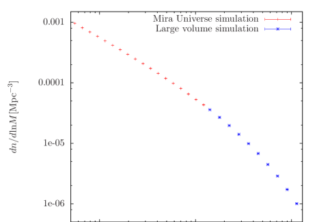
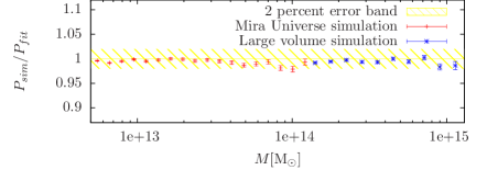
Figure 8: Upper panel: Mass function including Poisson error bars from the Mira-Titan Universe simulation (red) to cover the low mass end of the mass function and an additional large volume simulation, spanning a (5664 Mpc)³ volume (blue) to cover the cluster regime. Lower panel: Ratio of the simulation results with respect to the Bhattacharya et al. (2011) fit, assuming universality. The yellow shaded region shows the 2% error band.

The mass range of interest for cosmological surveys in the area of “cluster cosmology” actually covers the range from galaxy groups to large clusters. With a mass resolution of $m_{p}\sim 1.05\cdot 10^{10}$M_⊙ for the $\Lambda$CDM case, the Mira-Titan Universe comfortably resolves this range of masses. With a volume of (2100Mpc)³ the number of very massive clusters is not very large, and we therefore limit the use of the Mira-Titan Universe run to a mass range between $m_{\rm halo}\sim 5\cdot 10^{12}$M_⊙ to $m_{\rm halo}\sim 1\cdot 10^{14}$M_⊙. For the small mass end, halos are therefore resolved with $\sim 500$ particles which minimizes the need for (FOF) mass corrections due to undersampling of the halos. For the high-mass halos, this cut ensures that we have tens of thousands of halos in the relevant mass bins. In order to cover the upper end of the mass function, we employ another set of simulations. These simulations cover volumes of $\sim$ 5600Mpc³ and evolve 4096³ particles, leading to a mass resolution of $m_{p}\sim 10^{11}$M_⊙. These simulations were designed to generate mock catalogs for surveys such as BOSS and DESI (Sunayama et al. in preparation). At masses of $m_{\rm halo}\sim 1\cdot 10^{14}$M_⊙ halos are resolved with $\sim 1000$ particles. If we restrict the mass range to $m_{\rm halo}\sim 10^{15}$M_⊙, the last mass bin has more 10,000 halos, leading to small statistical errors.

Figure 8 shows the results for the mass function from the Mira-Titan Universe simulation for the lower mass end and the results from the large simulation for the cluster regime. We use the friends-of-friends (FOF) definition for determining the halo masses using a linking length of $b=0.2$ (Davis et al. 1985). This mass function definition has been studied very thoroughly in the past and allows us to compare our results to other work. (Our discussion can easily be extended to overdensity masses as well.) The lower panel displays the ratio of the simulation results with respect to a mass function fit developed in Bhattacharya et al. (2011). The simulations agree with this fit to better than 2% (yellow band) over the full mass range.

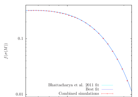
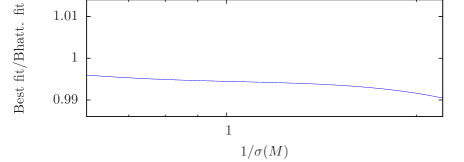
Figure 9: Upper panel: Combined simulation result (red) for $f(\sigma)$ compared to the best fit from Bhattacharya et al. (2011) and the best fit to the simulation result. The two fits are basically indistinguishable. Lower panel: Ratio between the two fits. The agreement is better than one percent.

The functional form of the Bhattacharya et al. (2011) fit is inspired by the original Sheth-Tormen mass function fit (Sheth & Tormen, 1999) but has one additional parameter and allows for explicit redshift dependence:

$$f^{\rm Bhatt}(\sigma,z)=A\sqrt{\frac{2}{\pi}}\exp\left[-\frac{a\delta_{c}^{2}}{2\sigma^{2}}\right]\left[1+\left(\frac{\sigma^{2}}{a\delta_{c}^{2}}\right)^{p}\right]\left(\frac{\delta_{c}\sqrt{a}}{\sigma}\right)^{q},$$ (16)

with the following parameters (note that all parameters are different from the original Sheth-Tormen choices):

$$A=\frac{0.333}{(1+z)^{0.11}};~{}~{}a=\frac{0.788}{(1+z)^{0.01}};~{}~{}p=0.807;~{}~{}q=1.795,$$ (17)

with $\delta_{c}=1.686$. Figure 9 shows the results for $f(\sigma(M))$ as a function of $1/\sigma(M)$ as measured by the combined simulations and the fit from Bhattacharya et al. (2011). We have refitted all parameters for $z=0$ using our current simulations and find extremely good agreement with the previous results:

$$A=0.3315\pm 0.0003;~{}~{}a=0.7895\pm 0.0085;$$ (18)

$$p=0.8148\pm 0.0451;~{}~{}q=1.8001\pm 0.0425,$$

shown in Figure 9. The agreement between the fits at the sub-percent (the lower panel in Figure 9 shows the ratio of the two fits) is rather remarkable and reassuring, given the fact that the simulations were carried out with different codes. Since the simulation results are very smooth already, we do not need to employ a special smoothing procedure. Instead, we will be able to build the emulator directly from the binned mass function datasets, eliminating one source of uncertainty in the emulator construction.

Next, we briefly discuss how to reduce the computational costs for the large simulation volume runs. In Sunayama et al. (in preparation) a detailed study is carried out concerning the number of time steps needed to obtain accurate predictions for halo statistics. In the HACC code the time stepper is divided into long time steps for the long-range force solver and each long time step is subdivided into shorter time steps with short-range force solves in order to resolve small scale structures accurately. At a mass resolution of $m_{p}\sim 10^{11}$M_⊙ and with the mass function as the observational target, the number of sub-cycles can be reduced without losing accuracy. Figure 10 shows the ratio of the mass function in the mass regime of interest for the large simulation with 2 and 5 sub-cycles (earlier tests shown in, e.g., Habib et al. (2016) have demonstrated convergence for 5 sub-cycles). The difference is at the sub-percent level, with computational costs reduced by a factor of 2.5. At the same time, these simulations will be still very useful for generating synthetic sky catalogs for large scale structure surveys such as DESI.

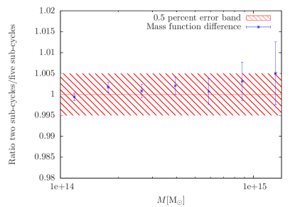
Figure 10: Mass function error in the regime of cluster masses due to coarsening the time stepping. Shown is the ratio of a simulation with 2 sub-cycles per long-range step over 5 sub-cycles. In the mass regime where the large volume runs will be used, the difference is at the sub-percent level. Given the computational saving of a factor of 2.5, this small inaccuracy is tolerable.

Our final mass function emulator will go beyond a single mass definition. We will measure mass functions from our simulations for both FOF and overdensity definitions, varying linking length and overdensity specification. This will make it more convenient to compare the results to observational mass measurements and proxies as well as to study connections between the different halo definitions. The extension of our results shown above to build a flexible emulator like this is straightforward.

Finally, we comment on the higher cluster mass range of the mass function. In this paper, we have been very conservative with regard to pushing the mass range too far. In future work, following the discussion in Lukić et al. (2007), we will include careful investigations on finite volume effects in our simulations allowing us to push to higher masses. We will provide a more detailed discussion on this topic in a forthcoming paper, where we focus solely on the mass function.

6.2 Emulator Performance

In order to test the emulator performance following the design strategy outlined in Section 3, we need a mass function surrogate – just as we used linear theory for the power spectrum. First suggested in Jenkins et al. (2001), writing the mass function in terms of $\sigma(M)$ allows for an almost universal description of the friends-of-friends (FOF) mass function for a linking length of $b=0.2$ that depends only on the linear power spectrum. Over time this universality has been investigated in detail (see, e.g., Reed et al. 2007; Cohn & White 2008; Lukić et al. 2007; Tinker et al. 2008; Crocce et al. 2010; Courtin et al. 2010; Bhattacharya et al. 2011) with the conclusion that for the specific definition of the $b=0.2$-FOF mass function, universality holds at the 10% level accuracy over a wide range of cosmologies. We use this result in the following to investigate the accuracy of a mass function emulator over the parameter space discussed in this paper.

We use the universal form of the mass function given in Eq. (17) by Bhattacharya et al. (2011) to generate mass function predictions for all our models. Figure 11 shows the model space covered by the simulation campaign described in this paper as well as the test cosmological models used to gauge the emulator accuracy. The $\Lambda$CDM model used throughout the paper is also shown.

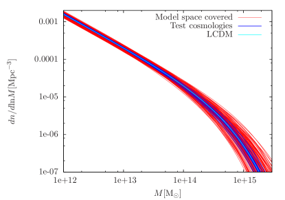
Figure 11: Coverage of mass function model space with the simulation design described in this paper at $z=0$ (red). The dark blue lines show the test models and the light blue line the fiducial $\Lambda$CDM mass function. All models are based on assuming universality is valid over the full parameter range. This assumption is valid at the $\sim 10\%$ level of accuracy.

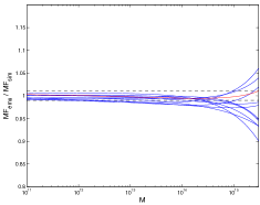
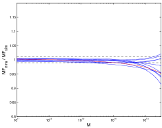
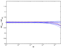
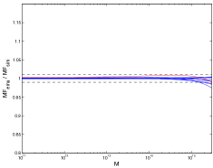
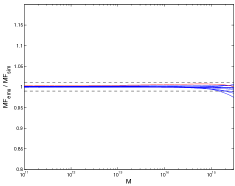
Figure 12: Emulator test: An emulator for the mass function is built from up to 101 and 111 models, assuming universality. Next, the mass functions for 10 additional models are predicted with the emulator and compared to the prediction assuming universality. Shown is the ratio of prediction to “truth”, the emulator predictions are accurate at the 1% level (dashed line) over the full mass range once 101 (111) models are considered. The upper panels show the prediction for emulator based on 26 and 36 models, the middle panels are based on 55 and 65 models, and for the predictions shown in the lower panels all 101 and 111 models were used. As before, the right panels include the addition 10 simulations with $m_{\nu}=0$.

Based on these mass function predictions, we build an emulator in the same way as for the power spectrum. Figure 12 shows the results for the emulator predictions for the test models at $z=0$. The first two panels show the results from an emulator based on 26 and 36 models. The accuracy of the emulator is already within 5%, a very encouraging result. Increasing the number of models to 55 (65 including the $m_{\nu}=0$ models) reduces the prediction error to $\sim 3\%$, and the final results for 101 and 111 models promise to yield inaccuracies at the 1% level over an 8-dimensional parameter space. This leads us to the conclusion that if the mass function prediction from the simulation can be provided at sufficient accuracy, building highly accurate emulators will be straightforward.

7 Beyond the Power Spectrum and Mass Function

7.1 Emulators

In the previous sections we have shown examples of two precision emulators to be built from the Mira-Titan Universe campaign targeted to impacting analysis of data from ongoing and upcoming dark energy surveys. The outlined simulation campaign lends itself to building many more emulators. One such example is a concentration-mass ($c-M$) emulator. In Kwan et al. (2013a) it was shown that an accurate $c-M$ emulator can be built from a small set of simulations – the paper was based on an augmented set of Coyote Universe simulations. The Mira-Titan Universe volume and mass and force resolution is sufficient to generate predictions for the $c-M$ relation over a mass range covering groups to cluster scales.

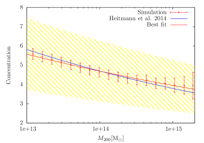
Figure 13: Concentration-mass relation as measured from the Mira-Titan Universe simulation (red points). The red line shows the best-fit power law through the simulation points. In blue we show the best fit $c-M$ relation found in the Q Continuum simulation (Heitmann et al. 2014), a simulation with almost 100 times better mass resolution, allowing the derivation of a fit out to much smaller halo masses. The yellow shaded region shows the intrinsic scatter. Within this scatter, the predictions from the Mira-Titan Universe simulation agree very well with the high-mass resolution Q Continuum simulation.

Figure 13 shows the $c-M$ relation measured from the Mira-Titan Universe run at $z=0$. Given the intrinsic scatter in the $c-M$ relation, the statistics obtained from the Mira-Titan Universe simulation are more than sufficient to derive accurate $c-M$ relation predictions over the mass range shown. Each halo here is resolved with at least 1000 particles to provide well-sampled halos when determining the concentration (for details about the concentration measurements, see Bhattacharya et al. 2013). For comparison, we show the best fit power law derived from the Q Continuum simulation Heitmann et al. (2014), a simulation with much higher mass resolution. The agreement is very good.

Another example is an emulator constructed for the galaxy power spectrum. In Kwan et al. (2013b), the Mira-Titan Universe simulation was used to build a galaxy power spectrum emulator covering a wide range of HOD models. With the complete suite of models we will be able to extend that work to not only cover different HOD models but to also provide predictions across cosmologies. Extending our work into redshift space is another obvious direction, as redshift space distortion power spectrum and correlation function emulators can be easily obtained based on the simulations outlined here.

7.2 Sky Maps

Beyond emulators, the simulation suite described here will also be very valuable for producing synthetic sky maps. For the LSST Dark Energy Science Collaboration we have generated an HOD-based galaxy catalog for the large scale structure working group. The size and resolution of the main simulations will also be sufficient to build weak lensing maps for surveys such as DES. Maps tracing the kinematic Sunyaev-Zel’dovich effect are currently being developed. We are planning to publicly release these maps to the community.

8 Conclusion

In this paper we have introduced the Mira-Titan Universe, a new simulation campaign to provide accurate predictions for a range of cosmological observables and for generating sky maps in different wavebands. This work is a major new extension of our previous Coyote Universe project in several key respects.

1. The cosmological parameter space covered is extended by three parameters, $w_{a}$, $h$, and $m_{\nu}$, all of which will play a central role in future analyses of dark energy surveys. We have shown that despite the extended parameter space the number of models needed to build reliable emulators is still manageable.

2. A new design strategy has been implemented using space-filling lattices. This strategy allows us to improve the emulator quality by systematically adding more simulations to an existing latice design. Our new strategy has the benefit of explicitly enforcing space-filling properties in intermediate stages as well as in the final design. We would like to stress that this procedure is highly nontrivial – extensive tests showed that simply adding independent space-filling designs (as in conventional Latin hypercube sampling) will not lead to the desired results.

3. We have extended our investigations beyond the power spectrum and demonstrated that our design will also provide high-accuracy emulators for the mass function. In addition, the simulation set will allow us to build a range of other emulators, for the halo concentration-mass relation, galaxy correlation functions and power spectra, and redshift space distortions.

4. We have demonstrated with a set of high resolution simulations that the needed requirements for such a simulation suite can be met. These simulations can then be also used for a range of other investigations, in particular building mock catalogs for different wavebands.

Table 2: Validation Set

Model	$\omega_{m}$	$\omega_{b}$	$\sigma_{8}$	$h$	$n_{s}$	$w_{0}$	$w_{a}$	$\omega_{\nu}$
E001	0.1433	0.02228	0.8389	0.7822	0.9667	-0.8000	-0.0111	0.008078
E002	0.1333	0.02170	0.8233	0.7444	0.9778	-1.1560	-1.1220	0.005311
E003	0.1450	0.02184	0.8078	0.6689	0.9000	-0.9333	-0.5667	0.003467
E004	0.1367	0.02271	0.8544	0.8200	0.9444	-0.8889	-1.4000	0.002544
E005	0.1400	0.02257	0.7300	0.7067	0.9889	-0.9778	-0.8444	0.009000
E006	0.1350	0.02213	0.8700	0.7633	0.9111	-1.0220	0.5444	0.000700
E007	0.1383	0.02199	0.7456	0.6500	0.9556	-1.1110	1.1000	0.007156
E008	0.1300	0.02286	0.7922	0.8011	1.0000	-1.0670	0.2667	0.006233
E009	0.1417	0.02300	0.7767	0.7256	0.9222	-0.8444	0.8222	0.004389
E010	0.1317	0.02242	0.7611	0.6878	0.9333	-1.2000	-0.2889	0.001622

References

- Abell et al. (2009) Abell, P. A. Allison, J., Anderson, S.F., et al. [LSST Science Collaborations and LSST Project Collaboration] 2009, arXiv:0912.0201 [astro-ph.IM]
- Ade et al. (2013) Ade, P.A.R., Aghanim, N., Armitage-Caplan, C., et al. [ Planck Collaboration] 2014, A&A, 571, 16
- Agarwal & Feldman (2011) Agarwal, S. & Feldman, H. 2011, MNRAS, 410, 1647
- Benson et al. (2000) Benson, A.J., Cole, S., Frenk, C.S., Baugh, C.M., & Lacey, C.G. 2000, MNRAS, 311, 793
- Bergner (2011) Bergner, S., 2011, Making choices in multi-dimensional parameter spaces, PhD thesis, Simon Fraser University
- Berlind & Weinberg (2002) Berlind, A.A. & Weinberg, D.H. 2002, ApJ, 575, 587
- Bhattacharya et al. (2011) Bhattacharya, S., Heitmann, K., White, M., Lukić, Z., Wagner, C., & Habib, S. 2011, ApJ 732, 122
- Bhattacharya et al. (2013) Bhattacharya, S., Habib, S., Heitmann, K., & Vikhlinin, A. 2013, ApJ 766, 32
- Bird et al. (2012) Bird, S., Viel, M., & Haehnelt, M.G. 2012, MNRAS, 420, 2551
- Brandbyge et al. (2008) Brandbyge, J., Hannestad, S., Haugbolle, T., & Thomsen, B. 2008, JCAP, 0808, 020
- Brandbyge & Hannestad (2009) Brandbyge, J. & Hannestad, S. 2009, JCAP, 0905, 002
- Brandbyge & Hannestad (2010) Brandbyge, J. & Hannestad, S. 2010, JCAP, 1001, 021
- Chevalier & Polarski (2001) Chevalier, M. & Polarski, D. 2001, Int. J. Mod. Phys. D, 10, 213
- Cohn & White (2008) Cohn, J. D., & White, M. 2008, MNRAS, 385, 2025
- Conway & Sloane (1999) Conway, J.H. & Sloane, N.J.A. 1999, Sphere Packings, Lattices and Groups. – 3rd ed, Springer
- Courtin et al. (2010) Courtin, J., Rasera, Y., Alimi, et al. 2010, MNRAS, 410, 1911
- Crocce et al. (2010) Crocce, M., Fosalba, P., Castander, F.J., & Gaztañaga, E. 2010, MNRAS, 403, 1353
- van Daalen et al. (2011) Daalen, M.P., Schaye, J., Booth C.M., & Vecchia C.D. 2011, MNRAS, 415, 3649
- Davis et al. (1985) Davis, M., Efstathiou G., Frenk, C.S. & White, S.D.M. 1985, ApJ, 292, 371
- Drinkwater et al. (2010) Drinkwater, M.J., Jurek, R.J., Blake, C., et al. 2010, MNRAS, 401, 1429
- Gardini et al. (1999) Gardini, A., Bonometto, S.A., & G. Murante 1999, ApJ, 524, 510
- Spergel (2015) Spergel, D., Gehrels, N., Baltay, C., et al. 2015, arXiv:1503.03757 [astro-ph.IM].
- Habib et al. (2007) Habib, S., Heitmann, K., Higdon, D., Nakhleh, C., & Williams, B. 2007, PhRvD, 76, 083503
- Habib et al. (2009) Habib, S., Pope, A., Lukić, Z., et al. 2009, J. Phys. Conf. Ser. 180, 012019
- Habib et al. (2012) Habib, S., Morozov, V., Finkel, H., Pope, A., et al. 2012, SC ’12 Proceedings of the International Conference on High Performance Computing, Networking, Storage and Analysis, Article No. 4, arXiv:1211.4864
- Habib et al. (2016) Habib, S., Pope, A., Finkel, H., et al. 2016, New Astronomy 42, 49
- Heitmann et al. (2006) Heitmann, K., Higdon, D., Nakhleh, C., & Habib, S. 2006, ApJ 646, L1
- Heitmann et al. (2009) Heitmann K., Higdon D., White M., et al. 2009, ApJ, 705, 156
- Heitmann et al. (2010) Heitmann K., White M., Wagner C., Habib S., & Higdon D. 2010, ApJ, 715, 104
- Heitmann et al. (2014) Heitmann K., Lawrence, E., Kwan, J., Habib, S., & Higdon, D. 2014 ApJ, 780, 111
- Heitmann et al. (2014) Heitmann, K., Frontiere, N., Sewell, C., et al. 2015, ApJ in press, arXiv:1411.3396
- Higdon (2002) Higdon, D. 2002, in Quantitative Methods for Current Environmental Issues, Space and Space-Time Modeling using Process Convolutions, ed. C. Anderson, V. Barnet, R.C. Chatwin, & A.H. El-Shaarawi (Berlin: Springer), 37
- Higdon et al. (2010) Higdon, D., Heitmann, K., Nakhleh, C., & Habib, S. 2010, The Oxford Handbook of Applied Bayesian Analyses, eds. A. O Hagan and M. West, 749
- Holsclaw et al. (2011) Holsclaw, T., Alam, U., Sansó, B., et al. 2011, PhRvD, 84, 083501
- Jenkins et al. (2001) Jenkins, A., Frenk, C.S., White, S.D.M., et al. 2001, MNRAS 321, 372
- Jing et al. (1998) Jing, Y.P., Mo, H.J., & Börner, G. 1998, ApJ, 494, 1
- Jing et al. (2006) Jing, Y.P., Zhang, P., Lin W.P., Gao L., & Springel, V. 2006, ApJ, 640, L119
- Johnson et al. (1990) Johnson, M.E., Moore, L.M., & Ylvisaker, D. 1990, Journal of Statistical Planning and Inference, 26(2), 131
- Kauffmann et al. (1997) Kauffmann, G., Nusser, A., & Steinmetz, M. 1997, MNRAS, 286, 795
- Klypin et al. (1993) Klypin, A. Holtzman, J., Primack, J., & Regos, E. 1993, Astrophys. J. 416, 1
- Komatsu et al. (2011) Komatsu, E., Smith, K.M., Dunkley, J. et al. 2011, ApJS, 192, 18
- Kwan et al. (2013a) Kwan, J., Bhattacharya, S., Heitmann, K., & Habib, S. 2013, Astrophys. J. 768, 123
- Kwan et al. (2013b) Kwan, J., Heitmann, K., Habib, S., et al. 2015, ApJ in press, arXiv:1311.6444
- Lawrence et al. (2010) Lawrence, E., Heitmann, K., White, M., et al. 2010 ApJ 713, 1322
- Lesgourgues et al. (2009) Lesgourgues, J., Matarrese, S., Pietroni, M., & Riotto, A. 2009, JCAP 0906, 017
- Lewis et al. (2000) Lewis, A., Challinor, A., & Lasenby, A. 2000, Astrophys. J. 538, 473
- Linder (2003) Linder, E. 2003, Phys. Rev. Lett. 90, 091301
- Lukić et al. (2007) Lukić, Z., Heitmann, K., Habib, S., Bashinsky, S., & Ricker, P.M. 2007, Astrophys. J., 671, 1160
- McKay et al. (1979) McKay, M.D., Beckman, R.J., & Conover, W.J. 1979, Technometrics, 21, 239
- Morris & Mitchell (1995) Morris, M.D., & Mitchell, T.J. 1995, Journal of Statistical Planning and Inference, 43, 381
- Morrison & Schneider (2013) Morrison, C.B. & Schneider, M. 2013, JCAP 11, 009
- Peacock & Smith (2000) Peacock, J.P., & Smith., R.E. 2000, MNRAS, 318, 1144
- Pietroni (2008) Pietroni, M. 2008, JCAP 10, 036
- Pope et al. (2010) Pope, A., Habib, S., Lukić, Z., et al. 2010, Comp. Sci. Eng. 12, 17
- Rasmussen & Williams (2006) Rasumussen, C.E. & Williams, K.I. 2006, Gaussian Processes for Machine Learning, MIT Press, www.GaussianProcess.org/gpml
- Reed et al. (2007) Reed, D., Bower, R., Frenk, C., Jenkins, A., & Theuns, T. 2007, MNRAS, 374, 2
- Refregier et al. (2010) Refregier, A., Amara A., Kitching, T. D., et al. 2010, arXiv:1001.0061 [astro-ph.IM].
- Riess et al. (2011) Riess, A., Macri, L., Casertano, S., et al. 2011, Astrophys. J. 730, 119
- Rudd et al. (2008) Rudd, D., Zentner, A., & Kravtsov, A. 2008, ApJ, 672, 19
- Sacks et al. (1989) Sacks, J., Welch, W.J., & Mitchell, T.J. 1989, Stat. Sci. 4, 409
- Santner et al. (2003) Santner, T.J., Williams, B.J., & Notz, W.I. 2003, The Design and Analysis of Computer Experiments, Springer, New York
- Schlegel, White, & Eisenstein (2009) Schlegel, D., White, M. & Eisenstein, D. 2009, arXiv:0902.4680 [astro-ph.CO]
- Schneider et al. (2008) Schneider, M., Knox, L., Habib, S., et al. 2008, PhRvD, 78, 063529
- Seljak (2000) Seljak, U. 2000, MNRAS, 318, 203
- Sheth & Tormen (1999) Sheth, R. & Tormen, G. 1999, MNRAS 308, 119
- Tinker et al. (2008) Tinker, J., Kravtsov, A.V., Klypin, A., et al. 2008, ApJ, 688, 709
- Upadhye et al. (2014) Upadhye, A., Biswas, R., Pope, A., et al. 2014, PhRvD, 89, 103515
- Viel et al. (2010) Viel, M., Haehnelt, M.G., & Springel, V. 2010, JCAP 1006, 015
- White (2004) White M. 2004, Astropart. Phys., 22, 211
- Zentner et al. (2008) Zentner, A.R., Rudd, D.H., & Kravtsov, A. 2008, PhRvD, 77, 043507
- Zentner et al. (2013) Zentner, A.R., Sembolini, E., Dodelson, et al. 2013, PhRvD, 87, 043509
- Zhan & Knox (2004) Zhan, H. & Knox, L. 2004, ApJ, 616, L75
- Zheng et al. (2005) Zheng, Z., Berlind, A., Weinberg, D.H., et al. 2005, ApJ, 633, 791