Novel opportunities for sub-meV inelastic X-ray scattering at high-repetition rate self-seeded X-ray free-electron lasers

Abstract

Inelastic X-ray scattering (IXS) is an important tool for studies of equilibrium dynamics in condensed matter. A new spectrometer recently proposed for ultra-high-resolution IXS (UHRIX) has achieved 0.6 meV and 0.25 nm^-1 spectral and momentum transfer resolutions, respectively. However, further improvements down to 0.1 meV and 0.02 nm^-1 are required to close the gap in energy-momentum space between high and low frequency probes. We show that this goal can be achieved by further optimizing the X-ray optics and by increasing the spectral flux of the incident X-ray pulses. UHRIX performs best at energies from 5 to 10 keV, where a combination of self-seeding and undulator tapering at the SASE-2 beamline of the European XFEL promises up to a hundred-fold increase in average spectral flux compared with nominal SASE pulses at saturation, or three orders of magnitude more than what is possible with storage-ring based radiation sources. Wave-optics calculations show that about $7\times 10^{12}$ ph/s in a $90$-$\mu$eV bandwidth can be achieved on the sample. This will provide unique new possibilities for dynamics studies by IXS.

I Introduction

Momentum resolved inelastic X-ray scattering (IXS) is a technique introduced [2, 3] and widely used [4, 5, 6, 7, 8] at synchrotron radiation facilities for studies of atomic-scale dynamics in condensed matter. IXS is a photon-in-photon-out method applicable to any condensed matter system, whether it is solid, liquid, biological, or of any other nature. A photon with energy $E_{{}_{\mathrm{i}}}$ and momentum $\mbox{\boldmath$K$}_{{}_{\mathrm{i}}}$ changes its energy and momentum to $E_{{}_{\mathrm{f}}}$ and $\mbox{\boldmath$K$}_{{}_{\mathrm{f}}}$ in an inelastic scattering process in the sample and leaves behind a collective excitation with energy $\varepsilon=E_{{}_{\mathrm{i}}}-E_{{}_{\mathrm{f}}}$ and momentum $\mbox{\boldmath$Q$}=\mbox{\boldmath$K$}_{{}_{\mathrm{i}}}-\mbox{\boldmath$K$}_{{}_{\mathrm{f}}}$, respectively, as shown in the sketch in Fig. 1. The interpretation of IXS is straightforward as it measures the dynamical structure factor $S(\mbox{\boldmath$Q$},\varepsilon)$, i.e. the spatiotemporal Fourier transform of the van Hove time-dependent pair correlation function [9]. Therefore, it provides access to dynamics on a length scale $\lambda=2\pi/Q$ and at a time scale $t=2\pi\hbar/\varepsilon$.

Figure 1: Time-length ($t-\lambda$) and energy-momentum ($\varepsilon\!-\!Q$) space of excitations relevant in condensed matter. The figure indicates how different domains are accessed by different inelastic scattering probes: neutrons (INS), X-rays (IXS), ultraviolet (IUVS), and Brillouin Light Scattering (BLS). The ultra-high-resolution IXS (UHRIX) spectrometer presented in Ref. [10] entered the previously inaccessible region marked in shaded green. The novel capabilities discussed in the present paper will enable IXS experiments with 0.1-meV and 0.02-nm^-1 resolution in the region marked in shaded light green. Hence, it allows to close the existing gap between the high-frequency and low-frequency probes. The energy $\varepsilon=E_{{}_{\mathrm{f}}}\!-\!E_{{}_{\mathrm{i}}}$ and the momentum $\mbox{\boldmath$Q$}=\mbox{\boldmath$k$}_{{}_{\mathrm{f}}}\!-\!\mbox{\boldmath$k$}_{{}_{\mathrm{i}}}$ transfers from initial to final photon/neutron states are measured in inelastic scattering experiments, as schematically shown in the inset.

IXS is one of only a few existing inelastic scattering techniques. Each technique provides access to a limited region in the time-length scale or equivalently in the energy-momentum space of collective excitations relevant for condensed matter. Figure 1 shows how a broad range of excitations are covered by different inelastic scattering probes: neutrons (INS), X-rays (IXS), ultraviolet light (IUVS), and Brillouin Light Scattering (BLS). A gap remains in experimental capabilities between low-frequency (visible and ultraviolet light) and high-frequency (X-rays and neutrons) inelastic scattering techniques. Hence, dynamics in the range from about 1-100 picosecond (ps) on atomic- and meso-scales is still inaccessible by any known experimental probe. This is precisely the region of vital importance for disordered systems and therefore many outstanding problems in condensed matter dynamics, such as the nature of the liquid to glass transition, could be addressed by entering this unexplored domain.

In principle there are no limitations preventing IXS from penetrating this unexplored dynamic range of excitations. This would, however, require solving two longstanding challenges in IXS. First, IXS spectrometers in their traditional implementation rely on an X-ray optics concept utilizing single-bounce Bragg back-reflecting spherical analyzers, leading to pronounced Lorentzian tails of the spectral resolution function. This approach has reached an impasse where the best numbers in energy ($\simeq 1.5$ meV) and momentum transfer ($\simeq 1.5$ nm^-1) resolutions have not improved for the past 20 years [11, 12]. Second, the IXS signal is very weak. For example, with $\simeq 10^{9}$ incident photons there is often less than one photon inelastically scattered into the detector. Hence, more efficient IXS spectrometers with better resolution and more powerful X-ray sources are required to advance the field.

Recently, a new type of dispersive spectrometer was tested for the first time. This ultra-high-resolution IXS (UHRIX) spectrometer [10] achieved a spectral resolution of 0.6 meV at a momentum transfer down to 0.25 nm^-1 (shaded green area in Fig. 1). Additionally, the spectral contrast improved by an order of magnitude compared to traditional IXS spectrometers [2, 13, 11, 14, 15, 12]. To sharpen the desired resolution to 0.1 meV and 0.02-nm^-1 and to ensure higher count rates, we propose to further develop the angular dispersive X-ray optical scheme [16, 17] replacing scanning IXS spectrometers with broadband imaging spectrographs [18] .

In addition to these optics developments, new types of X-ray sources are on the horizon that will overcome the problem of insufficient IXS cross-section by delivering a higher spectral flux, namely seeded high-repetition rate X-ray free-electron lasers (XFELs). Low-gain X-ray free-electron laser oscillators (XFELOs) may in some time in the future produce a spectral flux of up to $10^{14}-10^{15}$ photons/s/meV [20, 21], but currently they are still under conceptual development [22]. High-gain XFELs, on the other hand, are available today. Self-amplified spontaneous emission (SASE) X-ray free-electron lasers (XFELs) [23, 24, 25] deliver light pulses with unprecedented peak power compared to storage-ring based sources. However, the average photon flux that can be delivered is limited due to the low repetition rate of their linac drivers. By contrast, the European XFEL’s plan to adopt superconducting accelerator technology will allow for producing $27000$ X-ray pulses per second, i.e. orders of magnitude above the $120$ pulses per second of the LCLS and the $60$ pulses per second at SACLA.

The UHRIX instrument with the desired 0.1 meV resolution can be installed at the SASE-2 beamline of the European XFEL together with the MID instrument [26] operating in the 5-25 keV range. UHRIX performs best at relatively low photon energies between $5$ and $10$ keV with an optimum around $9$ keV. Owing to the high repetition rate of the European XFEL, the nominal average output flux at SASE-2 amounts to about $10^{12}$ photons/s/meV at 9 keV, which is more than one order of magnitude greater than at synchrotron radiation facilities [8]. Furthermore, the spectral flux can be substantially increased by self-seeding [27, 28], which at the European XFEL first will be available at the SASE-2 beamline [29]. Another order of magnitude increase in flux is achievable by tapering the magnetic field of the seeded undulator [30, 31, 32, 33, 34, 35, 36, 37]. We therefore propose an optimized configuration of the SASE-2 X-ray source combining self-seeding and undulator tapering techniques in order to reach more than $10^{14}$ photons/s/meV, the same number estimated in Ref. [38]. In combination with the advanced IXS spectrometer described here, this may become a real game-changer for ultra-high-resolution X-ray spectroscopy, for IXS in particular, and hence for the studies of dynamics in disordered systems.

The paper is organized as follows: in Section II we demonstrate that self-seeding, combined with undulator tapering, allows achieving the aforementioned figure of $10^{14}$ photons per second per meV bandwidth at the optimal photon energy range around 9 keV. This result is achieved by careful numerical modeling using the XFEL code GENESIS [39] and start-to-end simulations for the European XFEL. In Section III we introduce and evaluate the X-ray optical design to achieve 0.1 meV resolution IXS. The choice of optical elements and their design parameters are studied by dynamical theory calculations for monochromatization in Section III.1, and by geometrical optics considerations for X-ray focusing in Section III.3. The spectrograph design with a spectral resolution of 0.1 meV in a 5.8 meV wide spectral window of imaging is presented in Section III.4. The design parameters are verified in Section III.5 by wavefront propagation simulations from source to sample using a combination of GENESIS [39] and SRW [40] codes. All results are summarized and discussed in Section IV.

II High average flux X-ray source for Ultra-High-Resolution IXS

II.1 Concept

Figure 2: Schematic layout of the European XFEL accelerator providing electrons up to 17.5 GeV electron energy in a macro pulse pattern with 27000 pulses/s. Details of the HXRSS SASE-2 undulator are shown in Fig. 3.

Figure 3: Layout of SASE-2 undulator (35 segments) in the double-cascade self-seeding scheme for HXRSS. The monochromators are placed in the photon beam in between undulator segments where a magnetic chicane deviates the electrons.

This section describes a configuration of the SASE-2 X-ray source at the European XFEL, combining hard X-ray self-seeding (HXRSS) and undulator tapering techniques in order to optimize the average output spectral flux around $9$ keV, which is the optimum working point of the UHRIX setup. In its simplest configuration, a HXRSS setup consists of an input undulator and an output undulator separated by a chicane with a single crystal monochromator [27]. Like this, it has been implemented both at LCLS [28] and at SACLA [41]. The time structure of the European XFEL is characterized by $10$ macropulses per second, each macropulse consisting of $2700$ pulses, with $4.5$ MHz repetition rate inside the macropulse. The energy carried by each pulse and the performance of the crystal cooling system, removing deposited heat between macropulses, should conservatively satisfy the condition that during a macropulse, the drift in the central frequency of the crystal transmission function cannot exceed the Darwin width. Then, due to the high repetition rate of the European XFEL, the simplest two-undulator configuration for HXRSS is not optimal and a setup with three undulators separated by two chicanes with monochromators is proposed. This amplification-monochromatization double cascade scheme is characterized by a small heat load on the crystals and a high spectral purity of the output radiation [42] .

The figure of merit to optimize for IXS experiments is the average spectral photon flux. Here, the high-repetition rate of the European XFEL yields a clear advantage compared with other XFELs. However, even relying on its high repetition rate, the maximum output of the European XFEL is $10^{12}~{}\mathrm{{ph}}/\mathrm{s}/\mathrm{meV}$ in SASE mode at saturation, which is too low to satisfy the flux requirements discussed in the previous section. Therefore self-seeding and undulator tapering are needed.

The techniques proposed in this article exploit another unique feature of the European XFEL, namely its very long undulators. The SASE-2 line will feature $35$ segments, each consisting of a $5$ m long undulator with $40$ mm period. The 175 m SASE-2, undulator is much longer than required to reach saturation at $9$ keV (at $17.5$ GeV electron energy and $250$ pC pulse charge the saturation length amounts to about $60$ m). We exploit this additional length to operate the SASE-2 baseline in HXRSS mode followed by post-saturation tapering according to the scheme in Fig. 3, which has been optimized for our purposes.

Table 1: Operation parameters of the European XFEL used in this paper.

		Units
Undulator period	40	mm
Periods per segment	125	-
Total number of segments	35	-
K parameter (rms)	2.658	-
Intersection length	1.1	m
Wavelength	0.1358	nm
Energy	17.5	GeV
Charge	250	pC

Figure 4: Power distribution and spectrum of the X-ray pulse along the undulator: (a) and (b) calculated at the exit of the first undulator (5 segments); (c) and (d) after the first HXRSS monochromator; (e) and (f) at the exit of the second undulator (5 segments); (g) and (h) after the second HXRSS monochromator; (i) and (j) at the exit of the setup. Grey lines refer to single shot realizations, the black line refers to the average over one hundred simulations. The insets in (c) and (g) show an enlarged portion of the main plot, illustrating the seed appearing after the filtering process. The black arrows indicate the position of the seed relative to the electron slice with maximum current. The red lines in graphs (i) and (j) refer to the particular XFEL pulse that is used for wavefront propagation simulations (see Section III).

As discussed above, since we seek to combine the high repetition rate of the European XFEL with the HXRSS mode of operation, special care must be taken to ensure that the heat load on the crystal does not result in a drift in the central frequency of the transmission function of more than a Darwin width. A preliminary estimate [44] showed that in the case of radiation pulses with an energy of a few $\mu$J, the heat deposited could be removed by the monochromator cooling system without any problems . In order to keep the pulse energy impinging on the crystal within the few-$\mu$J range, one can exploit the double-cascade self-seeding setup in Fig. 3. The setup increases the signal-to-noise ratio, the signal being the seed pulse, competing with the electron beam shot noise. At the position of the second crystal, the seed signal is characterized by a much narrower bandwidth than the competing SASE signal leading to a much higher spectral density. In other words, in the frequency domain, the seed signal level is amplified with respect to the SASE signal by a factor roughly equal to the ratio between the SASE bandwidth and the seed bandwidth. One can take advantage of the increased signal-to-noise figure to reduce the number of segments in the first and second part of the undulator down to five, thus reducing heat load on the crystals due to impinging X-ray pulses. In the simulations we assume that the diamond crystal parameters and the (004) Bragg reflection are similar to those used for self-seeding at LCLS [28]. Optimization of crystal thickness and the choice of reflections may yield an increase in the final throughput [38]. However, here we will not be concerned with the optimization of the HXRSS setup in this respect.

II.2 Radiation from the SASE-2 undulator

We performed numerical simulations of the high average-flux source in Fig. 3 using the GENESIS code [39]. Simulations are based on a statistical analysis consisting of $100$ runs. Start-to-end simulations [43] yielded information about the electron beam (not shown) that is used as input for GENESIS. The parameters pertaining to the double-cascade self-seeded operation mode studied in this paper are shown in Table 1. The first five undulator segments serve as a SASE radiator yielding the output power and spectrum shown in Fig. 4(a) and (b), respectively. As explained in the previous Section, when working at high repetition rates it is critical to minimize the energy per pulse impinging on the diamond crystals. The energy per pulse can easily be evaluated integrating the power distribution in Fig. 4(a) yielding an average of about $1.2~{}\mu$J per pulse. As discussed in the previous Section, this level of energy per pulse is fully consistent with the proposed setup. The filtering process performed by the first crystal is illustrated in Fig. 4(c) and (d). The X-ray pulse then proceeds through the second undulator as shown in Fig. 3, where it seeds the electron beam.

Power and spectrum at the exit of the second undulator are shown in Fig. 4(e) and (f), respectively. This figure illustrates the competition between seed amplification and the SASE process, given the relatively low seeded pulse power from the first part of the setup. This is particularly evident in the time domain, where the seeded pulse follows about $20~{}\mu$m after the SASE pulse with almost similar power levels. Moreover, each of the pulses (seeded and SASE) carries about the same energy as the initial SASE pulse incident on the first crystal with a total incident average energy per pulse of about $2.7~{}\mu$J, i.e. still within the heat-load limits discussed in the previous Section. In the frequency domain a greatly increased peak power spectral density is observed for the seeded signal (compare Fig. 4(d) and (f)) while the SASE pulse contributes a wide-bandwidth, noisy background. The fact that the power spectral density for the seed signal is larger than for SASE by about an order of magnitude (roughly corresponding to the ratio of the SASE bandwidth to the seeded bandwidth) is what actually allows the X-ray beam to impinge on the second HXRSS crystal at low power, but with a large signal-to-noise (seeded-to-SASE) ratio, thus reducing heat loading effects by about one order of magnitude compared to a single-chicane scheme.

The filtering process performed by the second crystal is illustrated in Fig. 4(g) and (h), respectively. After this, the seed signal is amplified to saturation and beyond, exploiting a combination of HXRSS with post-saturation tapering.

Figure 5: Taper configuration for the output undulator (25 segments: 8 uniform, 16 tapered, 1 idle).

Figure 6: Energy (a) and variance (b) of energy fluctuations of the seeded FEL pulse as a function of the distance inside the output undulator. Grey lines refer to single shot realizations, the black line refers to the average over a hundred realizations.

Figure 7: Power (a) and spectrum (b) in the conventional SASE mode of operation at saturation, to be compared with power and spectrum in the HXRSS mode in Fig. 4(i) and (j), respectively. Grey lines refer to single shot realizations, the black line refers to the average over a hundred realizations.

Tapering is implemented by changing the $K$ parameter of the undulator, segment by segment according to Fig. 5. The tapering law used in this work has been implemented on an empirical basis, in order to optimize the spectral density of the output signal. The use of tapering together with monochromatic radiation is particularly effective, since the electron beam does not experience brisk changes of the ponderomotive potential during the slippage process.

Figure 8: Temporal, spectral, spatial, and angular distributions of the radiation pulse at the FEL undulator exit ($z=74$ m in Fig. 9). (a) Pulse power, pulse duration is $\simeq 14$ fs (FWHM) (b) Spectrum, spectral bandwidth is $\simeq 0.95$ eV (FWHM). (c) Spatial distribution, 2D plot; (d) vertical cut through the center of the fluence distribution; and (e) horizontal cut. The beam size is about $50~{}\mu$m (V)$\times 50~{}\mu$m (H) (FWHM). (f) Angular distribution, 2D plot; (g) vertical cut through the center of the fluence distribution; and (h) horizontal cut. The beam divergence amounts to $1.8~{}\mu$rad (V)$\times 1.8~{}\mu$rad (H) (FWHM).

The energy and variance of energy fluctuations of the seeded FEL pulse as a function of the distance inside the output undulator are illustrated in Fig. 6. On the average, pulses of about 11 mJ energy can be produced with this scheme. The final output of our setup is presented in Fig. 4(i) and (j), respectively, in terms of power and spectrum. This result should be compared with the output power and spectrum for SASE at saturation in Fig. 7 corresponding to the conventional operation mode foreseen at the European XFEL. Considering an average over $100$ shots, the peak power for the SASE saturation case in Fig. 7 is about $4\times 10^{10}$ W, while for the seeded case in Fig. 4(i), it has grown to $7.5\times 10^{11}$ W. This corresponds to an increase in flux from about $7\times 10^{11}$ photons per pulse to about $7\times 10^{12}$ photons per pulse. This amplification of about one order of magnitude is due to tapering. In addition, the final SASE spectrum has a FWHM of about $11.6$ eV, corresponding to a relative bandwidth of $1.2\times 10^{-3}$ while, due to the enhancement of longitudinal coherence, the seeded spectrum has a FWHM of about 0.94 eV, corresponding to a relative bandwidth of $1\times 10^{-4}$.

In conclusion, the proposed double-cascade self-seeding tapered scheme yields one order of magnitude increase in peak power due to undulator tapering, and a bit less than an order of magnitude decrease in spectral width due to seeding. Combining the two effects, we obtain an increase in spectral flux density of more that two orders of magnitude compared to saturated SASE ($2.1\times 10^{14}~{}\mathrm{{ph}}/\mathrm{s}/\mathrm{meV}$ compared to $1.5\times 10^{12}~{}\mathrm{{ph}}/\mathrm{s}/\mathrm{meV}$). The transverse beam size and divergence at the exit of the undulator are shown in Figs. 8(c)-(e) and 8(f)-(h), respectively. The beam profile is nearly circular with a size of about $50~{}\mu$m (FWHM) and a divergence of about $1.8~{}\mu$rad (FWHM). In the next section we will complement this information with detailed wavefront propagation simulations through the optical transport line up to the UHRIX setup.

III Optics for Ultra-High-Resolution IXS

The desired ultra-high-resolution IXS studies with 0.1 meV spectral and 0.02 nm^-1 momentum transfer resolution require a significant amount of X-ray photons with energy $E_{{}_{0}}=9.13185$ keV and momentum $K=E_{{}_{0}}/\hbar c=46.27598$ nm^-1 to be delivered to the sample within $\Delta E\lesssim 0.1$ meV spectral bandwidth and a transverse momentum spread $\Delta K\lesssim 0.02$ nm^-1, all concentrated on the sample in a spot of $\Delta s\lesssim 5~{}\mu$m (FWHM) diameter. The aforementioned photon energy $E_{{}_{0}}$ is fixed by the (008) Bragg reflection from Si single crystals, one of the central components of the ultra-high-resolution optics presented in detail below.

Figure 9: Main optical components of the proposed UHRIX instrument at the SASE-2-undulator beamline of the European XFEL shown schematically together with the output undulator. Optical components are presented as pictographs positioned at various distances from the effective source position in the SASE-2 undulator, 74 m upstream of the undulator exit. See text for descriptions.

We consider a scenario in which the UHRIX instrument is installed at the SASE-2-undulator beamline of the European XFEL. In particular, we consider an option of integrating UHRIX into the Materials Imaging and Dynamics (MID) station [26], an instrument presently under construction at the European XFEL. A schematic view of the optical components essential for delivering photons with the required properties to the sample is shown in Fig. 9. Optics are shown as pictographs in certain distances from the source. The effective source position is located around 74 m inside the undulator measured from the exit. This number was determined by back-propagation in free space of the XFEL radiation from the undulator end.

The main optical components are as follows: A biconcave parabolic refractive lens [45], creates a secondary source on the 6-bounce angular dispersive ultra-high-resolution CDDW+W monochromator. This is essential in order to achieve a tight focal spot on the sample because it eliminates the blurring that the strong angular dispersion of the CDDW+W monochromator would cause otherwise [18]. The CDDW+W monochromator then selects a 0.1 meV spectral bandwidth from the incident X-ray beam. The CDDW+W is a modification of a CDW-type angular dispersive monochromator  [46, 47, 17], which uses a three-step process of collimation (C), angular dispersion (D), and wavelength selection (W) [48]. Finally, a parabolic compound refractive lens CRL[49, 45] focuses the monochromatic X-rays on the sample.

The X-ray spectrograph captures photons scattered from the source in a sufficiently large solid angle and images them in a few-meV wide spectral window with 0.1-meV spectral resolution in the dispersion plane. The dispersing element (DE), a hard X-ray analog of an optical diffraction gratings, is a key component of the spectrograph. The spectrograph is also capable of simultaneously imaging scattered intensity perpendicular to the dispersion plane in a range of 0.2-nm^-1 with 0.01-nm^-1 resolution. Supplementary optical components include a pair of offset mirrors ($z$=349 m) which separate the beam from unwanted high-energy bremsstrahlung, and the two-bounce, two-crystal non-dispersive high-heat-load monochromator (HHLM at $z$=988 m). The HHLM narrows the 1 eV bandwidth of the incident X-rays to about 26 meV and thus reduces the heat-load onto the CDDW+W monochromator by a factor of 36.

In the remaining parts of this section, the choice of optical elements is justified and their design parameters are determined, first by using dynamical theory calculations for monochromatization with the X-ray crystal optics components in Section III.1 and then by applying ray transfer matrix formalism for ray tracing in Section III.3. The optical design is verified by wavefront propagation simulations using a combined application of GENESIS [39] and SRW [40] codes with results presented in Section III.5.

III.1 Monochromatization of X-rays

The radiation from the undulator discussed previously has about 950 meV bandwidth. It must be reduced to 0.1 meV and delivered to the sample with the smallest possible losses. To this end the previously discussed HHLM and CDDW+W are used in a two-tiered monochromatization scheme. In the following subsections we discuss their operating principles and design parameters in detail.

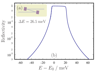
Figure 10: (a) Schematic view of the high-heat-load monochromator (HHLM). (b) Dynamical theory calculations of the spectral distribution of x rays around the nominal photon energy $E_{{}_{o}}=9.13185$ keV after two successive (115) Bragg reflections from diamond. The spectral bandwidth of the transmitted X-rays is 26.5 meV with a peak reflectivity of 97.7%. The angular spread of the incident X-rays is $\Delta\theta_{{}_{\mathrm{inc}}}=1~{}\mu$rad.

crystal/	$H$	$\eta_{{}_{H}}$	$\theta_{{}_{H}}$	$d$	$b_{{}_{H}}$	$\Delta E_{{}_{H}}$	$\Delta\theta_{{}_{H}}$
function
	$(hkl)$	[deg]	[deg]	[mm]		[meV]	[$\mu$rad]
C* / 1st	(1 1 5)	0	81.45	0.1	-1	33	24
C* / 2nd	(1 1 5)	0	81.45	0.3	-1	33	24

Table 2: Crystal and Bragg reflection parameters of the crystal elements of the HHL monochromator: $(hkl)$ - Miller indices of the Bragg diffraction vector $H$; $\eta_{{}_{H}}$ - asymmetry angle; $\theta_{{}_{H}}$ - glancing angle of incidence; $d$ - crystal thickness; $b_{{}_{H}}=-\sin(\theta_{{}_{H}}+\eta_{{}_{H}})/\sin(\theta_{{}_{H}}-\eta_{{}_{H}})$ - asymmetry parameter; $\Delta E_{{}_{H}}$ and $\Delta\theta_{{}_{H}}$ are the Bragg reflection’s intrinsic spectral width, and angular acceptance, respectively.

III.1.1 High-heat-load monochromator

A schematic of the high-heat-load monochromator (HHLM) is shown in Fig. 10(a). In the present design two diamond (C*) crystal plates are used as Bragg reflectors, with the (115) planes parallel to the crystal surface (symmetric Bragg). The (115) reflection is chosen for the Bragg angle to be as close as possible to $90^{\circ}$ (backscattering) for 9.13185 keV X-rays. This is dictated by stability requirements under high heat load, as the spectral variation of the reflected X-rays with incidence angle is minimized in back-scattering geometry. The Bragg reflection and crystal parameters used in the HHLM are provided in Table 2. Dynamical theory calculations of the spectral distribution of X-rays around the nominal photon energy $E_{{}_{o}}=9.13185$ keV after two successive (115) Bragg reflections from diamond are shown in Fig. 10(b).

III.1.2 High-resolution monochromator CDDW+W

The CDDW+W monochromator is a modification of the CDDW monochromator [47, 17, 10] complemented by two additional wavelength-selector crystals +W, ensuring a substantially reduced bandwidth and sharp Gaussian tails in the resolution function [50, 51, 16]. Figure 11(a) shows a schematic view of the CDDW+W monochromator, while Fig. 11(b) presents the results of dynamical theory calculations of the spectral distribution of X-rays after the CDDW+W. The crystal parameters used in the calculations are given in Table 3. The nominal photon energy $E_{{}_{0}}$=9.13185 keV of the UHRIX instrument is determined by the (008) Bragg reflection from the Si dispersion crystals D₁ and D₂ with a Bragg angle of $\theta=89.5^{\circ}$.

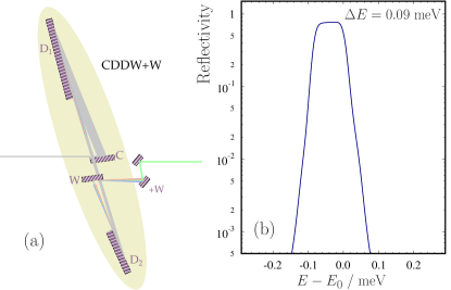
Figure 11: (a) Schematic view of the CDDW+W monochromator. (b) Dynamical theory calculations of the spectral distribution of x rays after six successive reflection from the crystals of the CDDW+W optic. Calculations were performed for incident X-rays around the nominal photon energy $E_{{}_{0}}=9.13185$ keV, with an angular spread of $1~{}\mu$rad and crystal parameters as in Table 3. The peak reflectivity of the optic is 71% with a spectral bandwidth of 0.09 meV.

crystal/	$H$	$\eta_{{}_{H}}$	$\theta_{{}_{H}}$	$d$	$b_{{}_{H}}$	$\Delta E_{{}_{H}}$	$\Delta\theta_{{}_{H}}$	${\mathcal{D}}_{{}_{H}}$
function
	$(hkl)$	[deg]	[deg]	[mm]		[meV]	[$\mu$rad]	[$\mu$rad
								meV]
C* / C	(3 3 1 )	-48	56.06	0.5	-0.14	124	20	-0.1
Si /D${}_{{}_{1}}$	(8 0 0 )	87.5	89.5	10	-1.5	22	280	6.2
Si /D${}_{{}_{2}}$	(8 0 0 )	87.5	89.5	10	-1.5	22	280	-6.2
C* / W	(3 3 1 )	48	56.05	0.5	-6.9	18	2.9	0.9
C* / +W	(4 0 0 )	0	49.57	0.5	-1.0	75	10	0
C* / +W	(4 0 0 )	0	49.57	0.5	-1.0	75	10	0

Table 3: Elements of the CDDW+W optics with their crystal and Bragg reflection parameters. Similar definitions are used as in Table 2. In addition, ${\mathcal{D}}_{{}_{H}}$ is the Bragg reflection’s dispersion rate. The cumulative asymmetry parameter and dispersion rate of the monochromator are $b_{\cup_{{}_{6}}}=2.25$, and ${\mathcal{D}}_{\cup_{{}_{6}}}=112~{}\mu$rad/meV, see definition in Table 4. The X-ray photon energy is $E_{{}_{0}}=9.13185$ keV.

III.2 Focusing optics

Because of the very large distances $l_{{}_{1}}$ and $l_{{}_{2}}$ a single 2D parabolic Be lens [45], denoted in Fig. 9 as “lens”, is sufficient to focus X-rays onto the CDDW+W monochromator. A lens with 1.68 mm radius ($R$) at the parabola apex, a focal distance $f_{\mathrm{lens}}=R/2\delta=205.5$ m, and with 1.5-mm geometrical aperture is considered in the following. The corrections $\delta=4.08684\times 10^{-6}$ and $\beta=1.4201\times 10^{-9}$ to the refractive index $n=1-\delta-{\mathrm{i}}\beta$ [52] are used in the wavefront propagation calculations.

The CRL at $z$=1017.5 m, see Fig. 9, focuses X-rays from the secondary source at the CDDW+W monochromator onto the sample. In preliminary wavefront propagation simulations an idealized system will be considered consisting of $N=39$ lenses each of 152.75 $\mu$m radius $R$ and all placed at the same position. The total focal length of the lens assembly is $f_{\mathrm{lens}}=R/2N\delta=0.479$ m. In the final calculations a more realistic extended CRL will be used containing 41 individual lenses separated by a 3 mm distance, with the first 39 having a 150 $\mu$m radius, and the last two a 400 $\mu$m radius at the parabola apex. The geometrical aperture of the CRL is 1 mm, which does not truncate the incident wavefront. All lenses are assumed to be perfect.

III.3 Focal spot size and momentum spread on the sample - analytical ray tracing

We use the ray-transfer matrix technique [53, 54, 55] to propagate paraxial X-rays through the optical system of the UHRIX instrument and to determine linear and angular sizes of the X-ray beam along the optical system. In a standard treatment, a paraxial ray in any reference plane (a plane perpendicular to the optical axis $z$) is characterized by its distance $x$ from the optical axis, by its angle $\xi$ with respect to that axis, and the deviation $\delta E$ of the photon energy from a nominal value $E$. The ray vector $\mbox{\boldmath$r$}_{{}_{1}}=(x,\xi,\delta E)$ at an input reference plane (source plane) is transformed to $\mbox{\boldmath$r$}_{{}_{2}}=\hat{O}\mbox{\boldmath$r$}_{{}_{1}}$ at the output reference plane (image plane), where $\hat{O}=\{ABG,CDF,001\}$ is a ray-transfer matrix of an optical element (elements) placed between the planes. The upper rows of Table 4 present the ray transfer matrices of the major components of the UHRIX optical system. The ray transfer matrix $\hat{U}$ of the UHRIX instrument, which describes propagation from the source to the sample, is presented in the last row of Table 4. We refer to Ref. [18] for details about the derivation of these matrices and provide here only essential notation and definitions.

In the focusing system, see the matrix $\hat{F}(l_{{}_{2}},f,l_{{}_{1}})$ in Table 4, a source in a reference plane at a distance $l_{{}_{1}}$ upstream of a lens with focal length $f_{{}_{12}}$ is imaged onto the reference image plane located at a distance $l_{{}_{2}}$ downstream from the lens. If the parameter $\Delta_{{}_{12}}$ defined in Table 4 equals zero, the classical lens equation ${l_{{}_{1}}}^{-1}+{l_{{}_{2}}}^{-1}={f_{{}_{12}}}^{-1}$ holds. In this case, the system images the source with inversion and a magnification factor $\mu_{{}_{2}}=1/\mu_{{}_{1}}=-l_{{}_{2}}/l_{{}_{1}}$ independent of the angular spread of rays in the source plane.

In the ray transfer matrix $\hat{C}(b,s{\mathcal{D}})$ describing Bragg reflection from a crystal at angle $\theta$, the asymmetry factor $b$ determines how the beam size and divergence change upon Bragg reflection. The angular dispersion rate ${\mathcal{D}}$ describes how the photon energy variation $\delta E$ from a nominal value $E$ changes the reflection angle with a fixed incident angle. The Bragg reflecting atomic planes are assumed to be at an asymmetry angle $\eta$ with respect to the crystal surface.

The ray transfer matrix $\hat{C}_{n}(b_{\cup_{{}_{n}}},{\mathcal{D}}_{\cup_{{}_{n}}})$ describing successive Bragg reflections from a system of $n$ crystals, has the same structure as that of a single Bragg reflection. The only difference is that the asymmetry parameter $b$ and the angular dispersion rate ${\mathcal{D}}$ are substituted by the appropriate cumulative values $b_{\cup_{{}_{n}}}$ and ${\mathcal{D}}_{\cup_{{}_{n}}}$, respectively. The ray transfer matrices of the offset mirrors and of the HHLM consisting of two symmetric Bragg reflections ($\eta=0$, $b=-1$, ${\mathcal{D}}=0$) (see Table 2) are unit matrices, leading to no change in the beam parameters.

Optical system	Ray-transfer matrix $\{ABG,CDF,001\}$	Definitions and Remarks
Focusing system	$\hat{F}(l_{2},f_{{}_{12}},l_{1})=$ $\left(\begin{array}[]{ccc}\mu_{{}_{2}}&\Delta_{{}_{12}}&0\\ -\frac{1}{f_{{}_{12}}}&\mu_{{}_{1}}&0\\ 0&0&1\end{array}\right)$	$\Delta_{{}_{12}}=l_{{}_{1}}+l_{{}_{2}}-\frac{l_{{}_{1}}l_{{}_{2}}}{f_{{}_{12}}}$ $\mu_{{}_{2}}=1-\frac{l_{{}_{2}}}{f_{{}_{12}}}=-\frac{l_{{}_{2}}-\Delta_{{}_{12}}}{l_{{}_{1}}}$ $\mu_{{}_{1}}=1-\frac{l_{{}_{1}}}{f_{{}_{12}}}=-\frac{l_{{}_{1}}-\Delta_{{}_{12}}}{l_{{}_{2}}}$
Bragg reflection from a crystal	$\hat{C}(b,s{\mathcal{D}})=$ $\left(\begin{array}[]{ccc}{1}/{b}&0&0\\ 0&b&s{\mathcal{D}}\\ 0&0&1\end{array}\right)$	$b=-\frac{\sin(\theta+\eta)}{\sin(\theta-\eta)}$ ${\mathcal{D}}=-(1/E)(1+b)\tan\theta$ $s=-1$ for clockwise, and $s=+1$ for counterclockwise ray deflection
Successive Bragg reflections from $n$ crystals	$\hat{C}_{n}(b_{\cup_{{}_{n}}},{\mathcal{D}}_{\cup_{{}_{n}}})=\hat{C}(b_{n},s_{n}{\mathcal{D}}_{n})\dotsb\hat{C}(b_{1},s_{1}{\mathcal{D}}_{1})$ $\left(\begin{array}[]{ccc}1/b_{\cup_{{}_{n}}}&0&0\\ 0&b_{\cup_{{}_{n}}}&{\mathcal{D}}_{\cup_{{}_{n}}}\\ 0&0&1\end{array}\right)$	$b_{\cup_{{}_{n}}}=b_{1}b_{2}b_{3}\dotsc b_{n}$ ${\mathcal{D}}_{\cup_{{}_{n}}}=b_{n}{\mathcal{D}}_{\cup_{{}_{n-1}}}+s_{n}{\mathcal{D}}_{n}$ $s_{i}=\pm 1$, $i=1,2,...,n$
UHRIX	$\hat{U}=\hat{F}(l_{{}_{4}},f_{{}_{34}},l_{{}_{3}})\hat{C}_{6}({\mathcal{D}}_{\cup_{{}_{6}}},b_{\cup_{{}_{6}}})\hat{F}(l_{{}_{2}},f_{{}_{12}},l_{{}_{1}})=$ $\left(\begin{array}[]{ccc}\frac{\mu_{{}_{2}}\mu_{{}_{4}}}{b_{\cup_{{}_{6}}}}-\frac{b_{\cup_{{}_{6}}}\Delta_{{}_{34}}}{f_{{}_{12}}}&\frac{\Delta_{{}_{12}}\mu_{{}_{4}}}{b_{\cup_{{}_{6}}}}+\Delta_{{}_{34}}\mu_{{}_{1}}b_{\cup_{{}_{6}}}&\Delta_{{}_{34}}{\mathcal{D}}_{\cup_{{}_{6}}}\\ -\frac{\mu_{{}_{2}}}{f_{{}_{34}}b_{\cup_{{}_{6}}}}-\frac{\mu_{{}_{3}}b_{\cup_{{}_{6}}}}{f_{{}_{12}}}&-\frac{\Delta_{{}_{12}}}{b_{\cup_{{}_{6}}}f_{{}_{34}}}+\mu_{{}_{1}}\mu_{{}_{3}}b_{\cup_{{}_{6}}}&\mu_{{}_{3}}{\mathcal{D}}_{\cup_{{}_{6}}}\\ 0&0&1\end{array}\!\!\!\!\!\right)$

Table 4: Ray-transfer matrices for a focusing system, for Bragg reflection from crystals, and for the complete optical system of the UHRIX instrument from source to sample.

The total ray transfer matrix $\hat{U}$ of the UHRIX instrument is a product of the ray transfer matrices of the lens focusing system $\hat{F}(l_{{}_{2}},f_{{}_{12}},l_{{}_{1}})$; the CDDW+W six-crystal matrix $\hat{C}_{6}(b_{\cup_{{}_{6}}},{\mathcal{D}}_{\cup_{{}_{6}}})$, and of the CRL focusing system $\hat{F}(l_{{}_{4}},f_{{}_{34}},l_{{}_{3}})$. The asymmetry parameters and the dispersion rate of the CDDW+W monochromator crystals required for the CDDW+W matrix are provided in Table 3. $\hat{U}$ describes propagation of X-rays in the vertical $(x,z)$ plane (see reference system in Fig. 9), in which the Bragg diffraction from the monochromator crystals takes place. Propagation of X-rays in the horizontal $(y,z)$ plane is not affected by Bragg diffraction from the monochromator crystals. Here, the appropriate UHRIX ray-transfer matrix is obtained from $\hat{U}$ with parameters $b_{\cup_{{}_{6}}}=1$ and ${\mathcal{D}}_{\cup_{{}_{6}}}=0$.

To determine the actual focal size and angular spread on the sample we use a linear source size (FWHM) $x_{{}_{0}}=y_{{}_{0}}=50~{}\mu$m, and an angular source size $\xi_{{}_{0}}=1.8~{}\mu$rad, as derived from the XFEL simulations in Section II. The energy spread of the X-rays is assumed $\delta E_{{}_{0}}=0.09$ meV. For the cumulative asymmetry parameter and dispersion rate of the CDDW+W monochromator we use $b_{\cup_{{}_{6}}}=2.25$, and ${\mathcal{D}}_{\cup_{{}_{6}}}=112~{}\mu$rad/meV as obtained from Table 3 and the distances between the optical elements are $l_{{}_{1}}=288$ m, $l_{{}_{2}}=718$ m, $l_{{}_{3}}=11.5$ m, and $l_{{}_{4}}=0.5$ m, see Fig. 9.

III.3.1 Focal spot size on the sample

The smallest focal spot size on the sample is achieved provided $\Delta_{{}_{12}}=0$, that is, the lens focuses X-rays on the CDDW+W monochromator, and $\Delta_{{}_{34}}=0$, meaning that the CRL refocuses X-rays on the sample with the secondary source on the CDDW+W monochromator. The focusing conditions require $f_{{}_{12}}=205.5$ m, and $f_{{}_{34}}=0.479$ m for the focal distances for the lens and CRL, respectively, see also Sec. III.2. In this case, the elements $B$ and $G$ of the $\hat{U}$ matrix are zero so the vertical and horizontal linear sizes of the source image on the sample are determined only by the element $A$:

$$x_{{}_{4}}=x_{{}_{0}}\mu_{{}_{2}}\mu_{{}_{4}}/b_{\cup_{{}_{6}}},\hskip 14.22636pty_{{}_{4}}=y_{{}_{0}}\mu_{{}_{2}}\mu_{{}_{4}}.$$ (1)

With $\mu_{{}_{2}}=-l_{{}_{2}}/l_{{}_{1}}=2.5$, and $\mu_{{}_{4}}=-l_{{}_{4}}/l_{{}_{3}}=0.044$, we obtain for the vertical spot size $x_{{}_{4}}=2.4~{}\mu$m, while for the horizontal size $y_{{}_{4}}=5.4~{}\mu$m. The vertical spot size $x_{{}_{4}}$ is less than half the target specification (5 $\mu$m) required to achieve 0.1 meV spectral resolution of the spectrograph [18], as discussed below in Section III.4. If focusing onto the CDDW+W is not perfect so that $\Delta_{{}_{12}}\not=0$, this may lead to an increase of the spot size by $\Delta x_{{}_{4}}=\xi_{{}_{0}}{\Delta_{{}_{12}}\mu_{{}_{4}}}/{b_{\cup_{{}_{n}}}}$ (resulting from element $B$ of the UHRIX ray-transfer matrix). However, this is not very critical, as even with a mismatch of $\Delta_{{}_{12}}\simeq 10$ m, the spot size increases only by an insignificant $\Delta x_{4}\simeq 0.4~{}\mu$m.

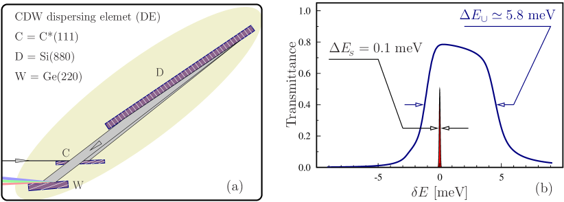
Figure 12: (a) The CDW-type three-crystal dispersing element of the spectrograph. (b) The spectral transmission function of the spectrograph with the CDW dispersing element ensuring a 5.8-meV broad window of imaging. The sharp line presents an 0.1-meV design spectral resolution of the spectrograph.

III.3.2 Transverse momentum spread

The transverse momentum spread in the diffraction plane (vertical) $\Delta K=K\xi_{{}_{4}}$ is defined by the angular spread

$$\xi_{{}_{4}}=\sqrt{(Cx_{{}_{0}})^{2}+(D\xi_{{}_{0}})^{2}+(F\delta E_{{}_{0}})^{2}}$$ (2)

of X-rays incident on the sample. Here we assume a Gaussian distribution of the beam parameters. In the vertical scattering plane the UHRIX ray-transfer matrix elements are $C=2.56~{}\mu$rad/$\mu$m, $D=21$, and $F=-2.58~{}\mu$rad/$\mu$eV. With $x_{{}_{0}}=50~{}\mu$m, $\xi_{{}_{0}}=1.8~{}\mu$rad, and $\delta E_{{}_{0}}=90~{}\mu$eV we obtain $\xi_{{}_{4}}=265~{}\mu$rad, and $\Delta K_{{}_{x}}=0.012$ nm^-1.

In the horizontal plane there is no angular dispersion. The cumulative dispersion rate ${\mathcal{D}}_{\cup_{{}_{6}}}=0$, and the asymmetry parameter $b_{\cup_{{}_{6}}}=1$. As a result, the angular dispersion related term $F=0$ and the only two nonzero elements are $C=5.31~{}\mu$rad/$\mu$m and $D=9$, resulting in $\xi_{{}_{4}}=266~{}\mu$rad and $\Delta K=0.012$ nm^-1. We note that both the vertical and the horizontal momentum spreads are smaller than the target specification $\Delta K=0.02$ nm^-1.

III.3.3 Pulse dilation

Bragg diffraction from an asymmetrically cut crystal with angular dispersion rate ${\mathcal{D}}$ inclines the X-ray intensity front by an angle $\beta=\arctan({\mathcal{D}}E)$ resulting in a pulse dilation $\delta t={\mathcal{D}}Ex/c$ [56] along the optical axis $z$. Here $x$ is the transverse pulse size after the angular dispersive optics and $c$ is the speed of light in vacuum. This effect is similar to wavefront inclination by optical diffraction gratings. The multi-crystal CDDW+W optic has a very large cumulative angular dispersion rate ${\mathcal{D}}_{\cup_{{}_{6}}}=112~{}\mu$rad/meV (see Table 2). The result is an inclination of the pulse intensity front by $\beta=\arctan({\mathcal{D}}E)=89.94^{\circ}$ and thus a very large pulse stretching $\delta t\,=\,{\mathcal{D}}_{\cup_{{}_{6}}}\,E\,x_{{}_{2}}/\,c=190$ ps (equivalent to a 57 mm pulse length). Here $x_{{}_{2}}=x_{{}_{0}}\mu_{{}_{2}}/b_{\cup_{{}_{6}}}=56~{}\mu$m is the vertical beam size after the CDDW monochromator.

III.4 Spectrograph

Spectral analysis of photons scattered from the sample is another important component of IXS spectrometers. Unlike monochromators, spectral analyzers should have a large angular acceptance, capable of collecting photons from the greatest possible solid angle (limited only by the required momentum transfer resolution), and with a spectral resolution matched to that of the monochromator. The spectral analyzer is usually the most difficult part of IXS spectrometers. In a standard approach the IXS analyzers measure sequentially one spectral point after another. A better strategy is to image the entire or a large part of the IXS spectra in single shots. Therefore, in the IXS instrument proposed here, the photon spectra are measured by an X-ray spectrograph. A spectrograph is an optical instrument that disperses photons of different energies into distinct directions and space locations, and images photon spectra on a position-sensitive detector. Spectrographs consist of collimating, angular dispersive, and focusing optical elements. Their principal schematic is shown in the pictograph of Fig. 9. Bragg reflecting crystals arranged in an asymmetric scattering geometry are used as dispersing elements (DE) of the hard X-ray spectrograph studied here [50, 51, 16, 18].

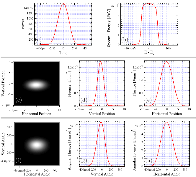
Figure 13: Temporal, spectral, spatial, and angular distributions of the radiation pulse on the sample ($z=1018$ m in Fig. 9). (a) Pulse power; the pulse duration is $\simeq 225$ ps (FWHM). (b) Spectrum; the spectral bandwidth is $\simeq 0.090$ meV (FWHM). (c) 2D plot of the spatial distribution. (d) Vertical cut through the maximum of the fluence distribution; and (e) horizontal cut. The beam size on the sample is $3.3~{}\mu$m (V)$\times 6.5~{}\mu$m (H) (FWHM). (f) Angular distribution, 2D plot; (g) vertical cut through the maximum of the fluence distribution; and (h) horizontal cut. Beam divergence on the sample is $220~{}\mu$rad (V) $\times~{}310~{}\mu$rad (H) (FWHM), corresponding to a $0.01$ nm${}^{-1}\times 0.015$ nm^-1 transverse momentum spread.

Several optical designs of hard X-ray spectrographs were proposed and their performances analyzed in Ref. [18]. Spectrographs with the desired target energy resolution of 0.1 meV and a spectral window of imaging up to a few tens of meVs were shown to be feasible for IXS applications. We refer to Ref. [18] for details. Here, we only briefly outline a particular spectrograph design with a DE consisting of three crystals in a CDW arrangement, schematically shown in Figure 12(a). Figure 12(b) shows the spectrograph’s spectral transmission function with a 5.8 meV wide window of imaging. The sharp line in the same figure represents the 0.1 meV design resolution.

location	$\Delta t$	$\Delta E$	$\Delta x$	$\Delta x^{\prime}$	$\Delta K_{{}_{x}}$	pulse	photons/	flux	spectral
(method)			$\Delta y$	$\Delta y^{\prime}$	$\Delta K_{{}_{y}}$	energy	pulse		flux
	ps	meV	$\mu$m	$\mu$rad	nm-1	$\mu$J	ph/pulse	ph/s	ph/s/meV
Undulator exit ($z$=74 m)	0.014	950	50	1.8	0	11000	$7.5\times 10^{12}$	$2.0\times 10^{17}$	$2.1\times 10^{14}$
(GENESIS)			50	1.8	0
sample ($z$=1018 m)	225	0.087	3.3	220	0.01	$0.33$	$2.3\times 10^{8}$	$6.3\times 10^{12}$	$7\times 10^{13}$
(SRW wavefront			6.5	310	0.015
propagation)
sample ($z$=1018 m)	190	0.09	2.4	265	0.012
(ray-transfer			5.5	266	0.012
matrix)

Table 5: Values (FWHM) of X-ray pulse parameters at different locations along the beamline in HXRSS mode with the UHRIX setup. See text for details. The total transmittance of the optics is 30% .

The spectral resolution of the spectrograph is given by

$$\Delta E_{{}_{\mathrm{S}}}=\frac{\Delta s}{f_{{}_{\mathrm{C}}}}\frac{|b_{\cup_{{}_{n}}}|}{{\mathcal{D}}_{\cup_{{}_{n}}}},$$ (3)

derived using the ray-transfer matrix formalism (see Section III.3 and Ref. [18]). A large cumulative dispersion rate ${\mathcal{D}}_{\cup_{{}_{n}}}$ of the dispersing element, a small cumulative asymmetry factor $|b_{\cup_{{}_{n}}}|$, a large focal distance $f_{{}_{\mathrm{C}}}$ of the collimating optics, and a small source size $\Delta s$ (beam size on the sample) are advantageous for better spectral resolution. For the three-crystal CDW dispersing element, with the optical scheme depicted in Fig. 12(a), we have $n=3$, ${\mathcal{D}}_{\cup_{{}_{3}}}=25~{}\mu$rad/meV, and $|b_{\cup_{{}_{3}}}|=0.5$. The target resolution of $\Delta E_{{}_{\mathrm{S}}}\lesssim 0.1$ meV is attained with $f_{{}_{\mathrm{C}}}=1$ m and $\Delta s\lesssim 5~{}\mu$m. The latter is in fact the origin of the target specification for the focal spot size on the sample discussed in the beginning of Section III. The estimated design value $x_{{}_{4}}=2.4~{}\mu$m, see Section III.3.1, is half the specification value and hence should yield a two times better spectral resolution than the 0.1 meV at target. For spectral imaging, focusing onto the detector is required only in one dimension. Hence, with a 2D position sensitive detector it is possible to simultaneously image the spectrum of X-rays along the vertical and the momentum transfer distribution along the horizontal axis.

III.5 Wavefront propagation through UHRIX optics

In this section the design parameters of the UHRIX are verified by wavefront propagation calculations. Physical optics simulations of the interaction of X-rays with the various optical elements of Figure 9 have been performed with the aid of two programs. The first, GENESIS [39], calculates the original wavefront of the SASE radiation at the exit of the output undulator, with the results presented in Section II.2. The second, SRW [40], calculates the wavefront after propagation from the undulator through drift spaces and optical components by using Fourier optics compatible local propagators. All together, including all lenses, crystals, and drift spaces, the beamline contains more than 100 elements. Simulations of the diffracting crystals with SRW have only recently become possible by addition of a new module [57] which also has been applied to the design of the planned IXS beamline at NSLS-II [58].

The temporal, spectral, spatial, and angular radiation pulse distributions and their parameters at the FEL undulator exit, $z=74$ m in Fig. 9, are given in Fig. 8. Radiation parameters (FWHM) such as pulse duration $\Delta t$, spectral width $\Delta E$, transverse size $\Delta x$, $\Delta y$; angular spread $\Delta x^{\prime}$, $\Delta y^{\prime}$, and transverse momentum spread $\Delta K_{{}_{x}}$, $\Delta K_{{}_{y}}$ are provided in captions to Fig. 8 and summarized in Table 5 together with peak and average flux values. The peak values are also a result of averaging over hundred runs with GENESIS, as discussed in Section II.2. The average flux values are obtained assuming a pulse repetition rate of 27 kHz.

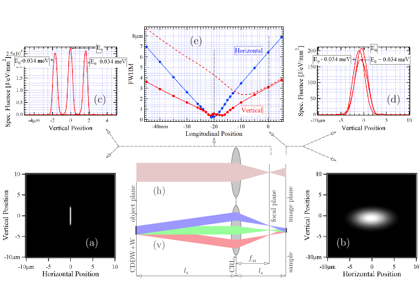
Figure 14: Fluence distributions and spot sizes of X-rays at different longitudinal positions near the sample. (a) Fluence distribution near the focal plane, and (b) in the sample (image) plane integrated over photon energies or pulse duration. (c) Vertical cuts through spectral fluence distributions at zero horizontal position for different spectral components near the focal plane (-20 mm), and (d) in the image plane (0 mm). (e) Vertical and horizontal spot sizes (FWHM) for the monochromatic radiation component $E_{{}_{0}}$ as a function of longitudinal position along the beam are presented by the solid lines. The red dashed curve in (e) represents the vertical size integrated over all spectral components. The optical scheme and schematic of ray propagation in the CRL focusing system are presented both in the vertical (v) and horizontal planes (h). The CDDW+W monochromator is in the object plane while the sample is in the image plane.

Results of the wavefront propagation simulations related to the sample area are presented graphically in Fig. 13. The temporal, spectral, spatial, and angular radiation pulse distributions and their parameters at the sample location (image plane), $z=1018$ m in Fig. 9, are provided in captions to Fig. 13 and summarized in Table 5 together with the peak and average flux values on the sample. The calculated radiation parameters at the sample location are in good agreement with values obtained by the ray-transfer matrix approach (Section III.3) which are shown for comparison in Table 5. They are also in agreement with the target specifications for the UHRIX instrument defined in Section III.

III.5.1 Spectral, spatial, and angular distribution

To avoid enlargement of the beam size on the sample due to the angular dispersion in the CDDW+W monochromator, it was proposed to place this monochromator in the object plane of the CRL, see Section III.3.1. This works perfectly in the geometrical optics approximation if the monochromator and the CRL are assumed to be point-like. (See Section III.3.1, and also the schematics in Fig. 14(v) and (h).) The question is how well this works with realistic sizes of monochromator crystals and of the individual lenses in the CRL, and with non-zero distances between all these elements. To address these issues, wavefront propagation simulations have been performed under realistic conditions. Detailed results are presented in Fig. 14, showing fluence distributions and spot sizes of X-rays at different longitudinal positions near the sample. There are striking differences in the transverse shape and sizes, integrated over all spectral components, in the image plane (Fig. 14(b)) and in the focal plane (Fig. 14(a)). There are equally striking differences in the positions and widths of the vertical beam profiles for different spectral components in the image plane (Fig. 14(d)) and in the focal plane (Fig. 14(c)).

The widths of the vertical pulse profiles (FWHM) for the monochromatic component $E_{{}_{0}}$ at different locations are presented in Fig. 14(e) by the red solid line. The blue solid line shows the widths of the horizontal profiles. The smallest widths $\lesssim 0.5~{}\mu$m of the vertical and horizontal monochromatic pulse profiles are achieved at $\simeq 21$ mm upstream of the sample position. This location coincides with the location of the focal plane, which is at a distance of $l_{{}_{4}}-f_{{}_{34}}=l_{{}_{4}}^{2}/(l_{{}_{3}}+l_{{}_{4}})=21$ mm from the CRL center, see sketch in Figs. 14(v) and (h). In the image plane the vertical width of approximately $3~{}\mu$m is much larger but all monochromatic profiles are almost at the same position so they probe the same scattering volume, as shown in Fig. 14(d). This is in agreement with the ray-transfer matrix calculations predicting zero linear dispersion in the image plane, as desired. In contrast, in the focal plane different monochromatic components are focused to much smaller sizes ($\simeq 0.5$ $\mu$m) but without spatial overlap, as shown in Fig. 14(c).

Figure 14(v) illustrates the origin of this behavior: Each monochromatic radiation component emanates from the CDDW+W monochromator (located in the first approximation in the object plane) with a very small angular spread $\lesssim 2~{}\mu$rad. Therefore, with a virtual source position practically at infinity they are focused onto the focal plane. Different monochromatic components emanate at different angles because of strong angular dispersion in the CDDW+W monochromator that eventually results in a linear dispersion in the vertical direction of the focal plane but no dispersion in the image plane, as required for UHRIX.

The horizontal transverse size of the X-ray pulse is independent of photon energy, since angular dispersion in the CDDW+W monochromator takes place only in the vertical plane. The smallest horizontal beam size is achieved near the focal plane with $\simeq 0.3~{}\mu$m (see Fig. 14(a) and Fig. 14(c)). This occurs because of the very small horizontal angular spread $\lesssim 1~{}\mu$rad of all X-ray spectral components emanating from the CDDW+W monochromator.

We note that the best position for the sample is actually neither in the image plane nor in the focal plane. As follows from the dependence presented by the dashed line Fig. 14(e) the smallest vertical beam size averaged over all spectral components is $\simeq 2.5~{}\mu$m and it is achived at about -10 mm from the image plane. The horizontal beam size at the same position is $\simeq 3.5~{}\mu$m. We also note that the extended (realistic 3D model) CRL described in Sec. III.2 does not introduce any substantial differences with respect to the initial simulations with an idealized, thin CRL.

III.5.2 Spatiotemporal distributions

The strong angular dispersion in the CDDW+W monochromator also causes substantial pulse dilation, as ray-transfer matrix calculations have shown in Section III.3.3. Here we present and discuss results of calculations of the spatiotemporal distributions of the X-ray pulses obtained by the wavefront propagation simulations.

The pulse duration at the exit of the undulator is only 15 fs (FWHM), as shown in Fig. 8. The pulse spectral bandwidth is $\simeq 950$ meV and it is reduced to $\Delta E=0.09$ meV (FWHM) by the crystal monochromators. Assuming a Gaussian spectral distribution after the CDDW+W monochromator, we obtain for the duration of a Fourier-transform-limited pulse $\Delta t=4\ln{2}\ \hbar/\Delta E=18.2$ ps (FWHM). The results of the calculations shown in Fig. 13 predict, however, a more than an order of magnitude larger pulse duration of $\simeq 225$ ps. This number agrees well with the duration calculated in Section III.3.3 as a result of the wave front inclination caused by angular dispersion in the CDDW+W monochromator.

III.5.3 Wavefront propagation summary

The wavefront propagation simulations confirm the soundness of the optical design of the UHRIX instrument worked out initially by the ray-transfer matrix approach and dynamical theory calculations. They also confirm the feasibility of the target specifications. The simulations show that the spectral flux from the XFEL undulator can be transported to the sample through the UHRIX X-ray optics with 30% efficiency reaching a remarkably high value of $\simeq 7\times 10^{13}$ ph/s/meV. This number exceeds by more than three orders of magnitude the spectral flux numbers reported for state-of-the-art IXS instruments at synchrotron radiation facilities [8]. Custom designed crystal and focusing optics ensure that on the sample $\simeq 6.3\times 10^{12}$ ph/s/meV photons can be concentrated in a spectral band of $0.09$ meV in a spot of $3.3({\mathrm{V}})\times 6.5({\mathrm{H}})~{}\mu$m² size and with a momentum transfer spread of $\lesssim 0.015$ nm^-1.

IV Discussion and Conclusions

This article explores novel opportunities for ultra-high-resolution IXS (UHRIX) at high repetition rate XFELs unlocked by the recent demonstration of a conceptually new spectrometer [10] with unprecedented specifications (0.6 meV spectral resolution and 0.25 nm^-1 momentum transfer), operating around $9$ keV. Its exploitation, together with the broadband ultra-high-resolution imaging spectrograph proposed in [18] will make it possible to fill the energy-momentum gap between high and low frequency inelastic probes and to provide exciting new opportunities for studies of dynamics in condensed matter. In particular, UHRIX experiments can be enabled at the European XFEL, where an increase of more than three orders of magnitude in average spectral flux is expected compared to what is available today at synchrotrons. The gain is due to two main factors: firstly, the high repetition rate of the European XFEL, owing to the superconducting linac accelerator driver, which allows up to 27000 X-ray pulses per second, and secondly, the presence of long undulators, allowing the combined implementation of hard X-ray self-seeding (HXRSS) and post-saturation tapering techniques. In particular, a double-chicane HXRSS scheme increases the signal-to-noise ratio and eases the heat-load on the HXRSS crystals to a tolerable level. This scheme is expected to yield up to TW-level X-ray pulses. Simulations of pulse propagation up to the sample position through the UHRIX optics show that an unprecedented average spectral flux of $7\times 10^{13}$ ph/s/meV is feasible. The power delivered to the sample can be as high as 350 W/mm² and radiation damage can become a limitation but liquid jets and scanning setups for solid samples can be employed to circumvent eventual problems, see Ref. [26] and references therein.

V Acknowledgments

We are grateful to Massimo Altarelli for many useful discussions and support, and to Thomas Tschentscher, Serguei Molodtsov, Harald Sinn, Stephen Collins, Giulio Monaco, Alexei Sokolov, Kwang-Je Kim, Kawal Sawhney, Alexey Suvorov and Igor Zagorodnov for useful discussions and interest in this work. Work at the APS was supported by the U.S. Department of Energy, Office of Science, Office of Basic Energy Sciences, under Contract No. DE-AC02-06CH11357. The development of SRW code is supported in part by the US DOE Office of Science, Office of Basic Energy Sciences under SBIR awards DE-SC0006284 and DE-SC0011237.

References

- [1]
- Burkel et al. [1987] E. Burkel, B. Dorner, and J. Peisl, Europhys. Lett. 3, 957 (1987).
- Burkel [1991] E. Burkel, Inelastic Scattering of X rays with Very High Energy Resolution, vol. 125 of Springer Tracts in Modern Physics (Springer, Berlin, 1991).
- Sette et al. [1998] F. Sette, M. H. Krisch, C. Masciovecchio, G. Ruocco, and G. Monaco, Science 280, 1550 (1998).
- Burkel [2000] E. Burkel, Rep. Prog. Phys. 63, 171 (2000).
- Krisch and Sette [2007] M. Krisch and F. Sette, Light Scattering in Solids IX (Springer, Berlin, 2007), vol. 108 of Topics in Applied Physics, chap. Inelastic X-ray Scattering from Phonons, pp. 317–370.
- Monaco [2015] G. Monaco, Synchrotron Radiation (Springer Berlin Heidelberg, 2015), chap. The High-Frequency Atomic Dynamics of Disordered Systems Studied by High-Resolution Inelastic X-ray Scattering, pp. 461–482.
- Baron [2015] A. Q. R. Baron, arXiv:1504.01098 (2015).
- Ashcroft and Mermin [1976] N. W. Ashcroft and N. D. Mermin, Solid State Physics (Holt, Rinehart and Witson, New York, 1976).
- Shvyd’ko et al. [2014] Y. Shvyd’ko, S. Stoupin, D. Shu, S. P. Collins, K. Mundboth, J. Sutter, and M. Tolkiehn, Nature Communications 5:4219 (2014).
- Masciovecchio et al. [1996] C. Masciovecchio, U. Bergmann, M. Krisch, G. Ruocco, F. Sette, and R. Verbeni, Nucl. Instrum. Methods Phys. Res. B 117, 339 (1996).
- Said et al. [2011] A. H. Said, H. Sinn, and R. Divan, Journal of Synchrotron Radiation 18, 492 (2011).
- Sette et al. [1995] F. Sette, G. Ruocco, M. Krisch, U. Bergmann, C. Masciovecchio, Mazzacurati, G. Signorelli, and R. Verbeni, Phys. Rev. Lett. 75, 850 (1995).
- Baron et al. [2001] A. Q. R. Baron, Y. Tanaka, D. Miwa, D. Ishikawa, T. Mochizuki, K. Takeshita, S. Goto, T. Matsushita, H. Kimura, F. Yamamoto, et al., Nucl. Instrum. Methods Phys. Res. A 467-468, 627 (2001).
- Sinn et al. [2001] H. Sinn, E. Alp, A. Alatas, J. Barraza, G. Bortel, E. Burkel, D. Shu, W. Sturhahn, J. Sutter, T. Toellner, et al., Nucl. Instrum. Methods Phys. Res. A 467-468, 1545 (2001).
- Shvyd’ko et al. [2013] Y. Shvyd’ko, S. Stoupin, K. Mundboth, and J. Kim, Phys. Rev. A 87, 043835 (2013).
- Stoupin et al. [2013] S. Stoupin, Y. V. Shvyd’ko, D. Shu, V. D. Blank, S. A. Terentyev, S. N. Polyakov, M. S. Kuznetsov, I. Lemesh, K. Mundboth, S. P. Collins, et al., Opt. Express 21, 30932 (2013).
- Shvyd’ko [2015] Y. Shvyd’ko, Phys. Rev. A 91, 053817 (2015).
- Trigo et al. [2013] M. Trigo, M. Fuchs, J. Chen, M. P. Jiang, M. Cammarata, S. Fahy, D. M. Fritz, K. Gaffney, S. Ghimire, A. Higginbotham, et al., Nature Physics 9, 790–794 (2013).
- Kim et al. [2008] K.-J. Kim, Y. Shvyd’ko, and S. Reiche, Phys. Rev. Lett. 100, 244802 (2008).
- Lindberg et al. [2011] R. R. Lindberg, K.-J. Kim, Y. Shvyd’ko, and W. M. Fawley, Phys. Rev. ST Accel. Beams 14, 010701 (2011).
- Maxwell et al. [2015] T. J. Maxwell, J. Arthur, Y. Ding, W. M. Fawley, J. Frisch, J. Hastings, Z. Huang, J. Krzywinski, G. Marcus, K.-J. Kim, et al., in Proceedings of the 2015 International Particle Accelerator Conference (SLAC Publication: SLAC-PUB-16286, 2015).
- Emma et al. [2010] P. Emma, R. Akre, J. Arthur, R. Bionta, C. Bostedt, J. Bozek, A. Brachmann, P. Bucksbaum, R. Coffee, F.-J. Decker, et al., Nature Photonics 4, 641 (2010).
- Ishikawa et al. [2012] T. Ishikawa, H. Aoyagi, T. Asaka, Y. Asano, N. Azumi, T. Bizen, H. Ego, K. Fukami, T. Fukui, Y. Furukawa, et al., Nature Photonics 6, 540–544 (2012).
- Altarelli et al. [2006] M. Altarelli, R. Brinkmann, M. Chergui, W. Decking, B. Dobson, S. Dusterer, G. Grübel, W. Graeff, H. Graafsma, J. Hajdu, et al., XFEL: The European X-ray Free-Electron Laser : Technical design report (DESY, Hamburg, 2006).
- Madsen et al. [2013] A. Madsen, J. Hallmann, T. Roth, and G. Ansaldi, Technical Design Report, XFEL.EU TR-2013-005, European X-ray Free-Electron Laser Facility GmbH, Hamburg, Germany (2013).
- Geloni et al. [2011a] G. Geloni, V. Kocharyan, and E. Saldin, Journal of Modern Optics 58, 1391 (2011a).
- Amann et al. [2012] J. Amann, W. Berg, V. Blank, F.-J. Decker, Y. Ding, P. Emma, Y. Feng, J. Frisch, D. Fritz, J. Hastings, et al., Nature Photonics 6 (2012).
- SXS [2014] XFELSEED, ‘Design and construction of Hard X-ray Self-Seeding Setups for the European XFEL’, Project approved in the framework of the coordinated German-Russian call for proposals ‘Ioffe-Röntgen Institute’ (2014).
- Sprangle et al. [1979] P. Sprangle, C.-M. Tang, and W. M. Manheimer, Phys. Rev. Lett. 43, 1932 (1979).
- Kroll et al. [1981] N. Kroll, P. Morton, and M. Rosenbluth, IEEE J. Quantum Electronics QE-17, 1436 (1981).
- Orzechowski et al. [1986] T. J. Orzechowski, B. R. Anderson, J. C. Clark, W. M. Fawley, A. C. Paul, D. Prosnitz, E. T. Scharlemann, S. M. Yarema, D. B. Hopkins, A. M. Sessler, et al., Phys. Rev. Lett. 57, 2172 (1986).
- Fawley et al. [2002] W. M. Fawley, Z. Huang, K.-J. Kim, and N. A. Vinokurov, Nucl. Instrum. Methods Phys. Res. A 483, 537 (2002).
- Wang et al. [2009] X. J. Wang, H. P. Freund, D. Harder, W. H. Miner, J. B. Murphy, H. Qian, Y. Shen, and X. Yang, Phys. Rev. Lett. 103, 154801 (2009).
- Geloni et al. [2010] G. Geloni, V. Kocharyan, and E. Saldin, arXiv:1007.2743 (2010), DESY 10-108.
- Fawley et al. [2011] W. Fawley, J. Frisch, Z. Huang, Y. Jiao, H.-D. Nuhn, C. Pellegrini, S. Reiche, and J. Wu, Tech. Rep., SLAC National Accelerator Laboratory, Menlo Park, CA 94025, USA (2011), SLAC-PUB-14616.
- Jiao et al. [2012] Y. Jiao, J. Wu, Y. Cai, A. W. Chao, W. M. Fawley, J. Frisch, Z. Huang, H.-D. Nuhn, C. Pellegrini, and S. Reiche, Phys. Rev. ST Accel. Beams 15, 050704 (2012).
- Yang and Shvyd’ko [2013] X. Yang and Y. Shvyd’ko, Phys. Rev. ST Accel. Beams 16, 120701 (2013).
- Reiche [1999] S. Reiche, Nucl. Instrum. Methods Phys. Res. A 429, 243 (1999).
- Chubar and Elleaume [1998] O. Chubar and P. Elleaume, EPAC-98 Proceedings pp. 1177–1179 (1998).
- Inagaki et al. [2014] T. Inagaki, T. Tanaka, N. Azumi, T. Hara, T. Hasegawa, Y. Inubushi, T. Kameshima, H. Kimura, H. M. R. Kinjo, A. Miura, et al., in Proceedings of FEL 2014 Conference (Basel, 2014), tUC01.
- Geloni et al. [2011b] G. Geloni, V. Kocharyan, and E. Saldin, arXiv:1109.5112 (2011b), DESY 11-165.
- Zagorodnov [2012] I. Zagorodnov (2012), http://www.desy.de/fel-beam/s2e/.
- Sinn [2012] H. Sinn (2012), private communication.
- Lengeler et al. [1999] B. Lengeler, C. Schroer, J. Tümmler, B. Benner, M. Richwin, A. Snigirev, I. Snigireva, and M. Drakopoulos, J. Synchrotron Radiation 6, 1153 (1999).
- Shvyd’ko et al. [2006] Y. V. Shvyd’ko, M. Lerche, U. Kuetgens, H. D. Rüter, A. Alatas, and J. Zhao, Phys. Rev. Lett. 97, 235502 (2006).
- Shvyd’ko et al. [2011] Y. Shvyd’ko, S. Stoupin, D. Shu, and R. Khachatryan, Phys. Rev. A 84, 053823 (2011).
- Shvyd’ko [2004] Y. Shvyd’ko, X-ray Optics – High-Energy-Resolution Applications, vol. 98 of Optical Sciences (Springer, Berlin Heidelberg New York, 2004).
- Snigirev et al. [1996] A. Snigirev, V. Kohn, I. Snigireva, and B. Lengeler, Nature 384, 49 (1996).
- Shvyd’ko [2011] Y. Shvyd’ko, arXiv:1110.6662 (2011).
- Shvyd’ko [2012] Y. Shvyd’ko, Proc. SPIE, Advances in X-ray/EUV Optics and Components VII 8502, 85020J (2012).
- Henke et al. [1993] B. L. Henke, E. M. Gullikson, and J. C. Davis, At. Data Nucl. Data Tables 54, 181 (1993).
- Kogelnik and Li [1966] H. Kogelnik and T. Li, Appl. Opt. 5, 1550 (1966).
- Matsushita and Kaminaga [1980] T. Matsushita and U. Kaminaga, Journal of Applied Crystallography 13, 472 (1980).
- Siegman [1986] A. E. Siegman, Lasers (University Science Books, Sausalito, California, 1986).
- Shvyd’ko and Lindberg [2012] Y. Shvyd’ko and R. Lindberg, Phys. Rev. ST Accel. Beams 15, 100702 (2012).
- Sutter et al. [2014] J. P. Sutter, O. Chubar, and A. Suvorov, Proc. SPIE 9209, 92090L (2014).
- Suvorov et al. [2014] A. Suvorov, Y. Q. Cai, J. P. Sutter, and O. Chubar, Proc. SPIE 9209, 92090H (2014).