Abstract

Tissue fusion eliminates physical voids in a tissue to form a continuous structure and is central to many processes in development and repair. Fusion events in vivo, particularly in embryonic development, often involve the purse-string contraction of a pluricellular actomyosin cable at the free edge. However in vitro, adhesion of the cells to their substrate favors a closure mechanism mediated by lamellipodial protrusions, which has prevented a systematic study of the purse-string mechanism. Here, we show that monolayers can cover well-controlled mesoscopic non-adherent areas much larger than a cell size by purse-string closure and that active epithelial fluctuations are required for this process. We have formulated a simple stochastic model that includes purse-string contractility, tissue fluctuations and effective friction to qualitatively and quantitatively account for the dynamics of closure. Our data suggest that, in vivo, tissue fusion adapts to the local environment by coordinating lamellipodial protrusions and purse-string contractions.

Introduction

Tissue fusion is a frequent and important event during which two facing identical tissues meet and bridge collectively over a gap before merging into a continuous structure (1). Imperfect tissue fusion in embryonic development results in congenital defects for instance, in the palate, the neural tube or the heart (1). Epithelial wound healing is another illustration of tissue fusion through which a gap in an epithelium closes to restore the integrity of the monolayer (2).

Model in vitro experiments have been developed using cell monolayers to study the different stages of healing from collective cell migration to the final stages of closure. In this context, we (3) and others (4, 5) have recently demonstrated that, for cells adhering to their substrate, and despite the presence of a contractile peripheral actomyosin cable at the free edge, the final stages of closure of wounds larger than a typical cell size result mostly from protrusive lamellipodial activity at the border. In that case, the function of the actin cable appears to be primarily to prevent the onset of migration fingers led by leader cells (6) at the free edge. Cell crawling has also been shown to have a major role in tissue fusion in vivo, for example during the closure of epithelial wounds in the Drosophila embryo (7).

However, in physiological developmental situations, there is often no underlying substrate to which lamellipodia can adhere to exert traction forces. This is the case, for instance, in neural tube formation (8) or in wound healing in the Xenopus oocyte (9). The generally well-accepted mechanism in these adhesion-free situations is the so-called purse-string mechanism in which the actomyosin cable at the edge of the aperture closes it by contractile activity (10). Note that the purse-string and the crawling mechanisms are not mutually exclusive (11) and may be involved at different stages of the closure (5, 12). In addition, "suspended" cohorts of cells, which do not interact with a substrate besides being anchored to a few discrete attachment points, are also observed in situations such as collective migration in cancer invasion (13).

Several experimental studies have documented protrusion-driven collective migration in vitro, but the purse-string mechanism has not been thoroughly investigated in model situations. Such an analysis imposes to suppress the contribution of the protrusions to closure and, therefore, to conduct the experiments on non-adherent substrates.

In a seminal paper, fibroblast sheets were shown to grow and migrate with their sides anchored to thin glass fibers (14). More recent studies extended this observation to keratinocyte monolayers or epidermal stem cells bridging between microcontact-printed adhesive tracks (15, 16). However, despite recent advances emphasizing the role of tissue remodeling (17), the mechanism of closure of a suspended epithelium in the absence of these anchoring sites remains an open question. To address this point, we have studied the dynamics of gap closure in an unsupported epithelium in which the actomyosin cable and the suspended tissue could not adhere to the substrate. Purse-string contractility in the absence of protrusions was therefore studied on well-defined mesoscopic non-adherent patches within an adherent substrate.

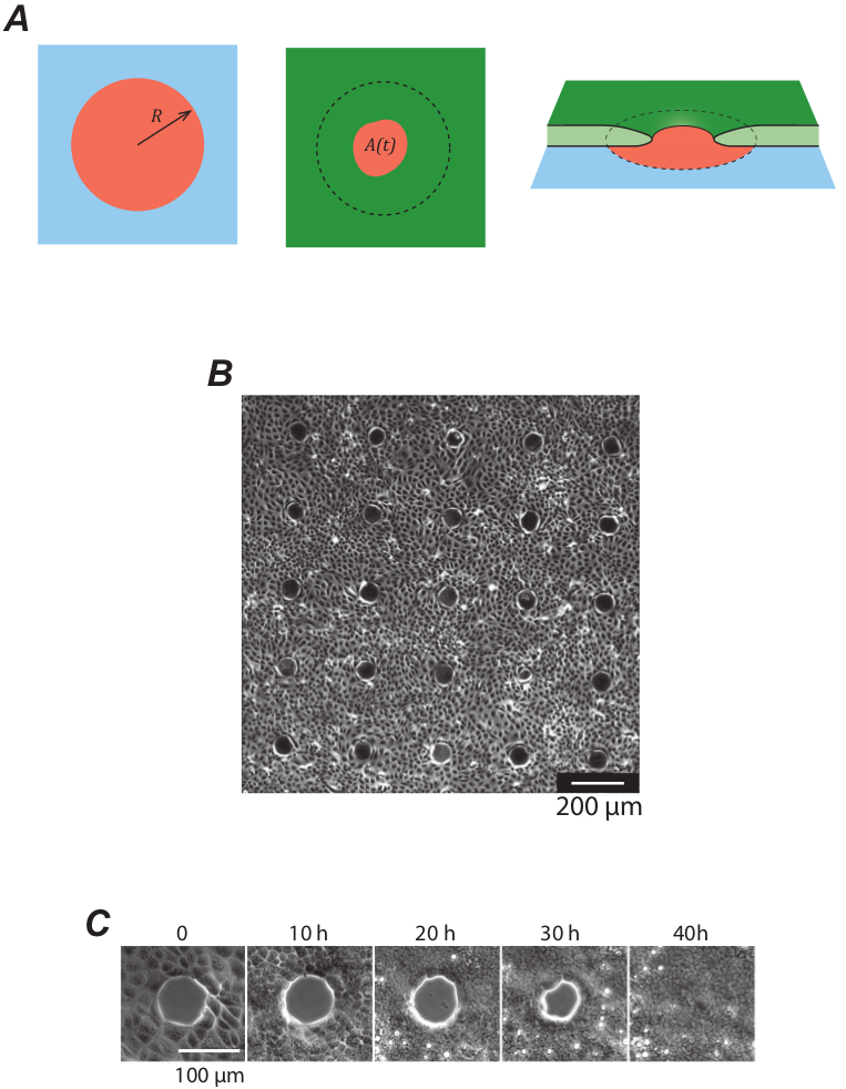
Figure 1: Fusion of an epithelium over non-adhering domains. A Schematics of the experiment: the surface (blue) is patterned with non-adhering domains (red) of radius $R$. Cells (green) progressively cover these domains and the cell-free area ($A(t)$) is dynamically monitored. B $5\times 5$ array of non- adhering domains in phase contrast at the onset of the experiment ($R=42\,\mu\mathrm{m}$). C Time evolution of a single domain ($R=42\,\mu\mathrm{m}$).

Results

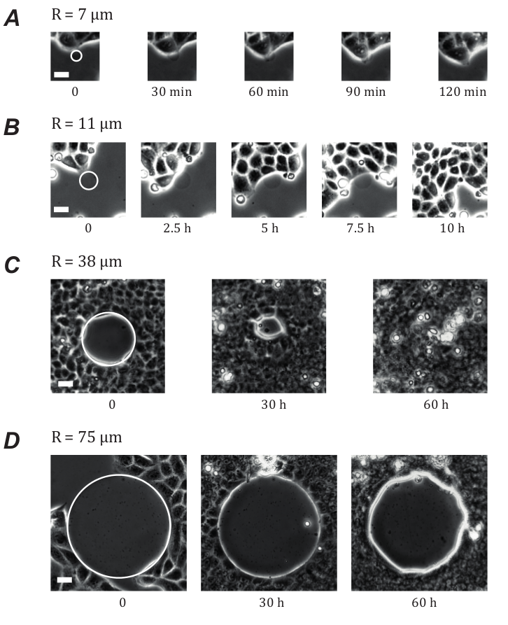
Figure 1: Behaviors of the monolayer according to the radius of the non-adherent domain. A Domains smaller than a cell size are covered rapidly with no arrest of the monolayer. B On domains whose size is comparable with a cell size, the monolayer stops before covering them rapidly as it progresses. C For still larger domains ($30\,\mu\mathrm{m}<R<65\,\mu$m), the monolayer surrounds the domains and then covers them by purse string as described in the text. D For domains larger than $70\,\mu$m, the monolayer surrounds the domains but cannot cover them.

We studied the bridging of a monolayer over a well-defined non-adherent gap on adherent glass substrates patterned with strictly non-adhesive circular regions of radius $R$ between $5$ and $75\,\mu$m (Figure 1A). The surface treatment kept its non-adherent properties for up to $3$ weeks in biological buffers (18, 19). To ensure we obtained reliable statistics, we worked with arrays of tens of non-adherent identical domains on which we cultured epithelial Madin Darby Canine Kidney (MDCK) cells (Figure 1B) (20). Notably, MDCK cell sheets have been previously shown to remain functional when suspended over large distances in culture medium (21). Fusion processes in neighbouring domains remained independent by imposing a space between each of at least $300\,\mu$m, a distance larger than the velocity correlation length measured independently for the same cellular system (22). Tissue fusion was monitored from confluence ($t=0$) up to $4$ days.

Immediately after seeding, the cells adhered on the glass and colonies developed by proliferation. The expanding monolayer readily covered non- adhesive domains that had a radius of less than $10\,\mu$m. In these cases, the advancing front edge made no arrest, confirming that cells have the ability to bridge over non-adherent defects smaller than their own size (23-26) (Supp. Figure 1). At the other extreme, for domains with a radius greater than $70\,\mu$m, the monolayer covered only the glass surface surrounding the patches (Supp. Figure 1). After several days, we observed the development of a tridimensional "rim" at the boundaries of the domains as already reported (19) but no further evolution in the subsequent weeks (19, 27).

Between these two limiting situations, the monolayer initially surrounded the non-adhesive domains and then proceeded to cover them until it eventually fused (Figure 1C, Supp. Figure 1, Supp. Video 1). Observations using confocal microscopy at the non-adherent surface / monolayer interface revealed the absence of vinculin or paxillin, two proteins associated with focal adhesions. This confirmed our basic assumption: the cells did not develop adhesions with the treated surface during and after closure (Supp. Figure 2).

We followed the closure process by monitoring the area covered by cells on domains of various sizes over a period of several days. A significant fraction of the domains with radii less than $30\,\mu$m were already closed when the monolayer reached confluence. Therefore, the mechanism by which cells cover these small domains may be different (for example by direct bridging) from the one relevant to larger domains. As a consequence, we limited our study to $30\,\mu\mathrm{m}<R<50\,\mu\mathrm{m}$. The cell-free area $A(t)$ showed only minor distortions to a quasi-circular shape, allowing us to define an effective radius $r(t)$ as $r(t)=\sqrt{A(t)/\pi}$ (Figure 1A).

It is worth comparing the present experiments with the healing of comparable size wounds of the same cell line on homogeneous adhesive substrates in which protrusions at the leading edge were shown to be the driving force for closure (3, 4). In both cases, the shape of the hole remained relatively circular; in particular, no fingering of the leading edge (6) was observed. However, the absence of cell-substrate adhesions drastically slowed down the closing dynamics (typically $30$ h in the present setting vs. $3$ h on a homogeneously adherent substrate for $R=35\,\mu$m). Moreover, in the experiments described here, the closing was very “noisy” in two respects. First, a given hole closed in a seemingly erratic succession of large amplitude retractions and expansions of the open area (Figure 2A). In some experiments, we observed closure down to $20\,\%$ of the initial radius, which then re-opened to $50\,\%$ before eventually closing. However, once the closure was fully completed, there was no re-opening (and no indication of a different morphology of the cells over the non-adhesive patch compared to the adhesive surface (Figure 1C)). Second, comparing several closure events for the same non-adhesive patch size, we observed a very large dispersion of the closure times (Supplementary Figure 3, Figure 2C-G). For instance, if $R=35\,\mu$m, the average closing time was $44$ h and the standard deviation was $18$ h ($N=150$). Because of this large dispersion, the entire distributions of the closure times (and therefore meaningful average closure times) after $83$ h could be accessed only for patches with a radius less than $35\,\mu$m. Unfortunately, the development of the above- mentioned 3D rim at the border after typically $4$ days prevented us from accessing the long-time parts of these distributions for larger domain sizes.

Given this large variability, we chose to reason in terms of the fraction $f(R,t)$ of closed holes at a time $t$ for a given initial radius $R$. This fraction $f$ is plotted as a function of $R$ after $4$ days (Figure 2H). As previously mentioned, all patches with a radius less than $35\,\mu$m closed within $83$ h. By contrast, only a small fraction of the experiments performed at $R>55\,\mu$m closed in this time-frame. As a matter of fact, we never observed the closing of patches whose radius was larger than $70\,\mu$m. The full dynamic evolution of these fractions is plotted as a heat map in Figure 3A for $30\,\mu\mathrm{m}<R<50\,\mu\mathrm{m}$ and $0<t<83$ h.

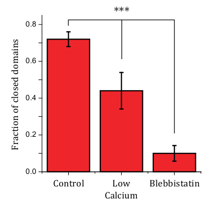
Figure 4: Importance of the monolayer cohesion and contractility. Low calcium conditions that lead to less cohesive monolayers resulted in a lower fraction of closed wounds as did the addition of Blebbistatin that almost halted the closure ($N_{\mathrm{control}}=125$, $N_{\mathrm{low}\,\mathrm{calcium}}=25$, $N_{\mathrm{blebbistatin}}=50$). $R=40\,\mu$m. Error bars are standard deviations.

Closure is necessarily a collective effect as cells must form a continuous structure that bridges over the non-adherent surface. Indeed, by conducting the experiments in low calcium conditions that disrupt cadherin-mediated cell-cell adhesions (19), the efficiency of closure was considerably reduced (Supp. Figure 4).

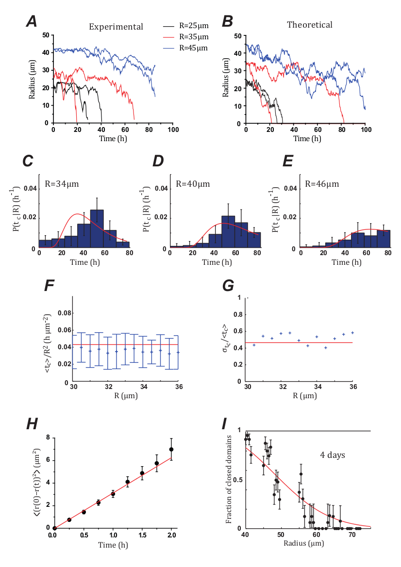
Figure 2: Gap closure is a stochastic process. A-B Comparison between experimental (A) and theoretical (B) trajectories. The two are visually very close. Note the very large fluctuations of the radius during closure. C-E The closure times are widely distributed for a given initial radius (bars: experimental values, lines theoretical predictions with $\tilde{\gamma}=10\;\mu\mathrm{m^{2}h^{-1}}$ and $D=1.6\;\mu\mathrm{m^{2}h^{-1}}$). Error bars are SEMs. $N$ values are $571$ (C), $498$ (D), $498$ (E). (F) As predicted by the model, the ratio $\langle t_{c}\rangle/R^{2}$ is approximately constant within the accessible dynamical range $30\leq R\leq 36\,\mu$m, where long time closure events ($t_{c}>84$h) are negligible. The red line corresponds to the theoretical prediction (Supp. Eq. (40)) $\frac{\langle t_{\mathrm{c}}(R)\rangle}{R^{2}}=\frac{1}{2(\tilde{\gamma}+D)}=0.043\mathrm{h}\mu\mathrm{m}^{-2}$ with $\tilde{\gamma}=10\;\mu\mathrm{m^{2}h^{-1}}$ and $D=1.6\;\mu\mathrm{m^{2}h^{-1}}$. Error bars are standard deviations. G The coefficient of variation of the closure time is approximately constant within the same range, with values consistent with the theoretical prediction (Supp. Eq. (46)) indicated with a solid line: $\frac{\sigma_{t_{\mathrm{c}}}({R})}{\langle t_{\mathrm{c}}(R)\rangle}=\left(\frac{2D}{3D+\tilde{\gamma}}\right)^{\frac{1}{2}}=0.47$ with $\tilde{\gamma}=10\;\mu\mathrm{m^{2}h^{-1}}$ and $D=1.6\;\mu\mathrm{m^{2}h^{-1}}$. H Early times are well described by a diffusive process. Points are the experimental points resulting from the average of more than $400$ trajectories, the red line is a linear fit yielding a diffusion coefficient of $D=1.56\pm 0.03\;\mu\mathrm{m^{2}h^{-1}}$ (error bars are SEMs). I Fractions of closed wounds at 4 days (black points). The red line is the theoretical fraction ($\tilde{\gamma}=10\;\mu\mathrm{m^{2}h^{-1}}$ and $D=1.6\;\mu\mathrm{m^{2}h^{-1}}$). Error bars are SEMs.

Figure 3: The fraction of closed wounds is well described by a stochastic model. A Experimental and B theoretical fractions of the closed wounds as a function of the initial radius $R$ and time $t$. The theoretical heatmap B is plotted with the values $\tilde{\gamma}=10\;\mu\mathrm{m^{2}h^{-1}}$ and $D=1.6\;\mu\mathrm{m^{2}h^{-1}}$ that correspond to the smallest error in the fit of the data (C). The two heatmaps are visually very close. C Plane of the error landscape (logarithmic scale). The cross denotes the optimum, the red contour bounds the $95\,\%$ confidence region. D The closure half-time is the time at which half of the wounds have closed. The points are the experimental data ($3825$ domains) and the line is the theoretical time for $\tilde{\gamma}=10\;\mu\mathrm{m^{2}h^{-1}}$ and $D=1.6\;\mu\mathrm{m^{2}h^{-1}}$. The fraction of closed patches at the end of the experiment is less than $0.5$ above $R=45\,\mu$m. Error bars are SEMs.

No stable lamellipodial protrusions similar to those observed on adherent surfaces were evidenced in the present experiments. Moreover, confocal imaging confirmed the presence of a pluricellular actomyosin cable at the edge of the closing open area (Figure 4). The contractility of this cable was tested with two-photon laser photo-ablation experiments and by inhibiting myosin II with blebbistatin. When severed, the cable retracted within a few tens of seconds (Figure 4B, C, Supp. Video 2), indicating that it is under mechanical tension. By contrast, when the epithelium bridging over the non-adherent surface was punctured after closure, the hole did not expand upon ablation, indicating that no significant tension is stored in the monolayer itself. These small wounds then closed rapidly by developing protrusions presumably on the debris left by the ablation. Furthermore, the addition of blebbistatin almost completely inhibited closure (Supp. Figure 4), whereas the same conditions have been shown to slow down but not halt closure on homogeneous adherent surfaces (4).

Our observations confirm that, as the cells do not interact with the surface in our experiments, the contractile pluricellular actomyosin cable along the edge must contract and pull the tissue over the adhesion-free surface by a purse-string mechanism. By contrast, the tension in the epithelium itself is not a factor in this process.

To describe these experiments, we wrote the force balance equation at the free edge, on a line element of the contractile cable of radius $r(t)$. As ingredients of the equation, we considered (Supp. Figure 5): 1/ a force $f_{\mathrm{cable}}=-\gamma/r$ due to the line tension $\gamma$ of the contractile cable, similar to what has been proposed to describe the shape of single cells anchored to the surface via discrete points (28, 29); 2/ a friction force $f_{\mathrm{friction}}=-\xi\,\mathrm{d}r/\mathrm{d}t$ where $\xi$ is a friction coefficient encapsulating the dissipative processes at the cable and between cells (there is no interaction and hence no friction at the monolayer/substrate interface); and 3/ a stochastic force $f_{\mathrm{noise}}$ needed to model the above-described stochastic effects, such as the wide distributions of closing times (Figure 2C-G, Supp. Figure 3) or the very noisy trajectories (Figure 2A). As puncturing the epithelium did not result in opening of the wound, we initially did not include epithelial tension in our description (see below). After dividing the force balance equation by the friction coefficient $\xi$, the Langevin equation describing the evolution of the radius $r(t)$ reads (Supp. Note 1) (30):

$$\frac{\mathrm{d}r}{\mathrm{d}t}=-\frac{\tilde{\gamma}}{r}+\sqrt{2D}\,\eta(t)$$ (1)

where $\tilde{\gamma}=\gamma/\xi$ and $\sqrt{2D}\,\eta(t)$ is a noise term where the diffusion coefficient $D$ quantifies the amplitude of radius fluctuations at the margin. Note that the hypothesis of radial force balance is supported by independent force measurements on keratinocytes, showing that, close to the free edge, the orthoradial component of the traction stress remained small compared to the radial component during closure (17).

For the sake of simplicity, we further assumed that i/ $\eta(t)$ is a Gaussian white noise with an autocorrelation function $\langle\eta(t)\eta(t^{\prime})\rangle=\delta(t-t^{\prime})$ and that ii/ $\gamma$, $\xi$ and $D$ remained constant (independent of $r$ and $t$). Note that a constant diffusion coefficient $D$ corresponds to fluctuations $\Delta\sigma$ of the epithelial tension $\sigma$ about its average value (zero in the present case): $D=\Delta\sigma^{2}/(2\xi^{2})$ (see below).

During the early stages of fusion, equation (1) reduces to simple diffusion, and the initial mean square deviation reads (Supp. Note 4):

$$\langle(r(0)-r(t))^{2}\rangle_{t\to 0}=2Dt$$ (2)

The experimental data were in good agreement with this theoretical expression, yielding $D=1.56\pm 0.03\,\mu\mathrm{m}^{2}\mathrm{h}^{-1}$ (Figure 2I) and confirming a diffusive behavior of the radius at short times. Hence, the cable tension $\gamma$ does not contribute to the initial statistics that are fully determined by the fluctuations.

In this framework, the fraction of closed wounds $f(R,t)$ obeyed a backward Fokker-Planck equation (30) (see Supp. Notes) :

$$\frac{\partial{}}{\partial{t}}f(R,t)=-\frac{\tilde{\gamma}}{R}\,\frac{\partial{}}{\partial{R}}f(R,t)+D\,\frac{\partial^{2}{}}{\partial{R^{2}}}f(R,t)$$ (3)

which could be solved numerically for a given set of parameters and with boundary conditions in accord with our experimental observations: We imposed that $r=R$ was a reflecting boundary (a hole never opened beyond the area of the non-adhesive domain) and $r=0$ was absorbing (there was no re-opening after full closure). The closure time was then the time at which $r=0$ was first attained (first-exit time).

A least-squares method allowed us to fit the model to the data over the whole map of the fraction of closed wounds (31). Varying $R$ and $t$ at given $\tilde{\gamma}$ and $D$, we minimized the mean square standardized error between theoretical frequencies and experimental fractions (see Supp. Note 3 for the definition of the error function and a full description of the fitting procedure). This fit yielded the following estimates of the parameters (Figure 3A):

$$\tilde{\gamma}=10\;\mu\mathrm{m^{2}h^{-1}}\quad\mathrm{and}\quad D=1.6\;\mu\mathrm{m^{2}h^{-1}}$$

where the numbers between brackets give the $95\,\%$ confidence interval (Figure 3C). Note that the diffusion coefficient is consistent with our previous estimate based on the short-time evolution of the closure (Figure 2I). With these parameters, the simulated and experimental fractions seemed very similar as can be seen in Figure 3A,B. More quantitatively, the particular case of the closure half-time at which $50\,\%$ of the domains have closed as well as the distributions of closure times for various radii were indeed well-described by this set of parameters (Figure 3D, Figure 2C-G, Supp. Note 3). Finally, trajectories simulated from equation (1) (32) with the previously determined values of $\tilde{\gamma}$ and $D$ closely resembled the experimental ones (Figure 2A,B).

Altogether, we conclude that our stochastic model provides a self- consistent description of the closure dynamics. As the confidence intervals for $D$ and $\tilde{\gamma}$ exclude $0$, the description is also minimal in the sense that none of the components can be removed from the description.

Discussion

We have provided evidence that a cell monolayer can develop over non- adherent surfaces even when cells at the edge are not anchored to a substrate to pull on it. This property is the transposition at the tissue scale of a single cell’s ability to bridge over defects smaller than their own size. Experiments conducted in low calcium conditions or in presence of Blebbistatin show that such closures are the result of a collective behavior and that impairing the acto-myosin contractility, in particular at the purse-string cable, impairs this process.

The experimental results are well described by a stochastic model that includes the tension $\gamma$ of the circumferential actomyosin cable, an effective friction $\xi$ and the amplitude $D$ of the fluctuations of the radius reflecting the ones of the epithelial tension. Our theory therefore emphasizes the role and function of the purse-string contractility under these conditions. Interestingly, this purse-string mechanism is secondary to lamellipodial protrusions when the same MDCK cells are migrating on surfaces on which they can develop adhesions (3). As MDCK cells develop a peripheral actomyosin cable in both these situations, we conclude that the nature of the substrate on which cells migrate controls whether this cable has a regularization or a purse-string function.

From a typical value of the cable tension $\gamma=1-10$ nN (25, 33), the order of magnitude of the (one-dimensional) friction coefficient is $\xi=0.1-1\,\mathrm{nN}\mu\mathrm{m}^{-2}\mathrm{h}$. We can compare this value with the hydrodynamic two-dimensional friction coefficient measured for the same cells in a similar setting but on an adherent substrate (3): $\xi_{\mathrm{adh}}=10^{-3}\,\mathrm{nN}\mu\mathrm{m}^{-3}\mathrm{h}$. The characteristic length defined as $\xi/\xi_{\mathrm{adh}}$ is typically $100-1000\,\mu$m, consistent with the correlation length characterizing the collective migration of MDCK cells on glass (3, 22). Therefore, it is likely that the friction term originates mostly from the monolayer adhering to the glass around the non-adhesive domains.

An important (and intuitively unexpected) conclusion of our study is that fluctuations actively contribute to closing. This is particularly apparent at the onset of closing (short times) where fluctuations are actually the dominant term in the closure dynamics (equation (2)). Theoretical average closure times can be analytically computed as first-exit times and we obtain for the average closure time $\langle t_{c}(R)\rangle=R^{2}/2(\tilde{\gamma}+D)$ (Supp. Note 3), which shows immediately that, in a statistical sense, a non-zero diffusion coefficient accelerates the closure. The model further predicts that the standard deviation of the closure time is proportional to and of same order as the average value (Supplementary notes 3,4). Quantitatively, within our limited dynamical range, these predictions are borne out by data with the fitted parameters determined previously (Figure 2F,G). Last, we validate one of our hypotheses of a white noise in the diffusive term of the Langevin equation (1). We used the model, and the fitted parameters, to measure the experimental noise, and checked that the autocorrelation function of this noise decays rapidly with time, with a correlation time of the order of an hour (Supplementary Figure 6). Since experiments are performed over days, this confirms that the white noise approximation is indeed appropriate.

We then checked whether our initial assumption of not including the epithelial tension in equation (1), initially based on tissue photoablation experiments, could be further confirmed. A non-zero tension $\sigma$ would add a constant term $\tilde{\sigma}=\sigma/\xi$ to the drift coefficient on the right-hand side of the Langevin equation (1). As shown in Supp. Note 2, analyzing our data with these three parameters $(\tilde{\gamma},\tilde{\sigma},D)$ yielded a very small (negative) epithelial tension whereas the two other parameters retained values close to the ones previously determined (Supp. Figure 7A,B). Therefore, the epithelial tension can be safely omitted, suggesting that the time-scales involved in the fusion process are sufficiently long to allow elastic stresses to relax (34). Not surprisingly, putting $\tilde{\gamma}=0$ in this new equation led to a drastic decrease of the fraction of closed wounds at $83$ h in good agreement with our experimental observations in presence of Blebbistatin (Supp. Figure 4).

Next, we asked whether including fluctuations of the cable tension would better describe our experimental data than our current hypothesis in which these fluctuations arise only from the epithelial tension ($D$ independent of $r$). Assuming for simplicity that fluctuations in the monolayer tension and in the cable tension are not correlated, we expressed the diffusion coefficient as $D_{\mathrm{tot}}(r)=D+D_{\gamma}/r^{2}$ where $D$ and $D_{\gamma}$ are proportional to the (constant) amplitudes of the fluctuations of these two tensions. Fitting model to data within a three-dimensional parameter space $(\tilde{\gamma},D,D_{\gamma})$ allowed us to conclude that fluctuations in the cable tension could be ignored except for values of $r$ much smaller than a cell size (Supp. Notes 3 and Supp. Figure 7C,D). Of note, at these very small radius values ($r<1\,\mu$m), the fluctuations of the cable become dominant over both the fluctuations of the epithelial tension and the deterministic cable tension (Supp. Note 2). This regime corresponds to the very late stages of closure, which are, unfortunately, beyond our experimental time resolution. Apart from this regime, the noise term of the stochastic model therefore originates from fluctuations of the monolayer tension about its zero mean value. These fluctuations result from cell-level dynamics occurring over short time scales, such as rearrangements, divisions, or cells being pulled out from the adhesive part.

From the typical value of $\xi$ determined above, we can also estimate the magnitude of the active fluctuations of the epithelial tension: $\Delta\sigma^{2}_{\mathrm{active}}=2D\xi^{2}=10^{-2}-1\,\mathrm{nN}^{2}\,\mu\mathrm{m}^{-2}\,\mathrm{h}$. This is, to our knowledge, the first experimental measurement of this quantity. We can compare this value to the amplitude of tension fluctuations resulting from thermal noise: $\Delta\sigma^{2}_{\mathrm{thermal}}=2D_{\mathrm{thermal}}\xi^{2}$. As the total friction of the cable over its perimeter is $2\pi R\xi$, the amplitude of thermal radius fluctuations is $D_{\mathrm{thermal}}=k_{B}T/(2\pi R\xi)$ where $k_{B}$ is Boltzmann’s constant, $T\sim 300$ K and $R\sim 10\,\mu$m. Hence, $\Delta\sigma^{2}_{\mathrm{thermal}}=10^{-8}-10^{-7}\,\mathrm{nN}^{2}\,\mu\mathrm{m}^{-2}\,\mathrm{h}$ : the amplitude of the epithelial tension fluctuations is several orders of magnitude larger than that of the thermal tension fluctuations, as expected in these active cellular systems (35).

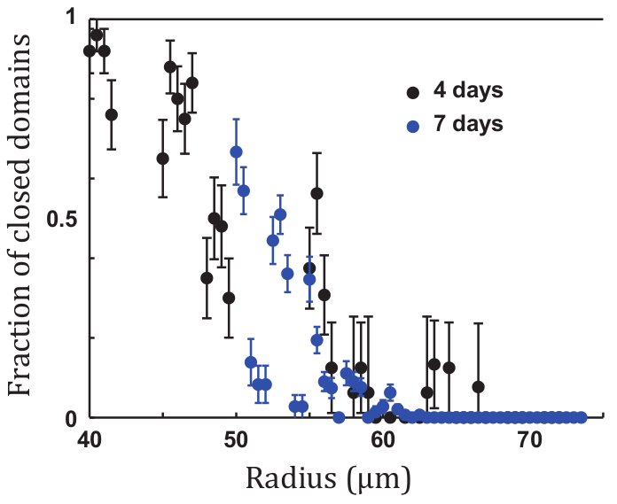
Figure 8: Long time behavior. Fractions of closed wounds at $4$ days (black points) and $7$ days (blue points). Because of the formation of a peripheral rim, there is no evolution after 4 days. Error bars are SEMs.

We end by considering tissue fusion over longer periods of time. A prediction of our model is that arbitrarily large wounds will always close, given an arbitrarily large duration, as the stochastic process defined by equation (1) yields trajectories that eventually always reach zero (36). Practically, however, because of the change of behavior induced by the 3D rim that develops at the adherent/non-adherent boundary, we stopped our analysis at $83$ h. Several arrays were further analyzed over longer time periods: at $4$ days, the evolution of the fractions of closed wounds was still well described by our model (Figure 2H). However, the closure process stopped after that time as we observed no evolution between $4$ and $7$ days (Supp. Figure 8), presumably due to rim formation at the edge even though the cells were still active and the border of the wounds was still fluctuating. This rim is likely to be the reason why large wound do not close in contrast with other cell types such as keratinocytes that are able to close gaps of several $100\,\mu$m (17).

In conclusion, we have shown that the collective migration of an epithelium can switch between two modes, depending on the cells’ affinity for their substrate. Whereas on adhesive surfaces, the collective migration is mostly driven by protrusions, our work shows that the purse-string mechanism is essential on non-adherent surfaces. Importantly, the active fluctuations of the tissue are also crucial and accelerate the closure dynamics. A natural future extension of our work will be to elaborate a more complete model where these active fluctuations are combined with the viscoelastic rheology of the tissue (17), to get a full description of the closure processes in more complex situations including, for example, in vivo tissue fusion in embryonic morphogenesis, or the collective migration of cancer cells in fibrillar environments (37). Other cell models may be better suited to address these important issues where gaps larger than the ones studied in the present work are to be closed.

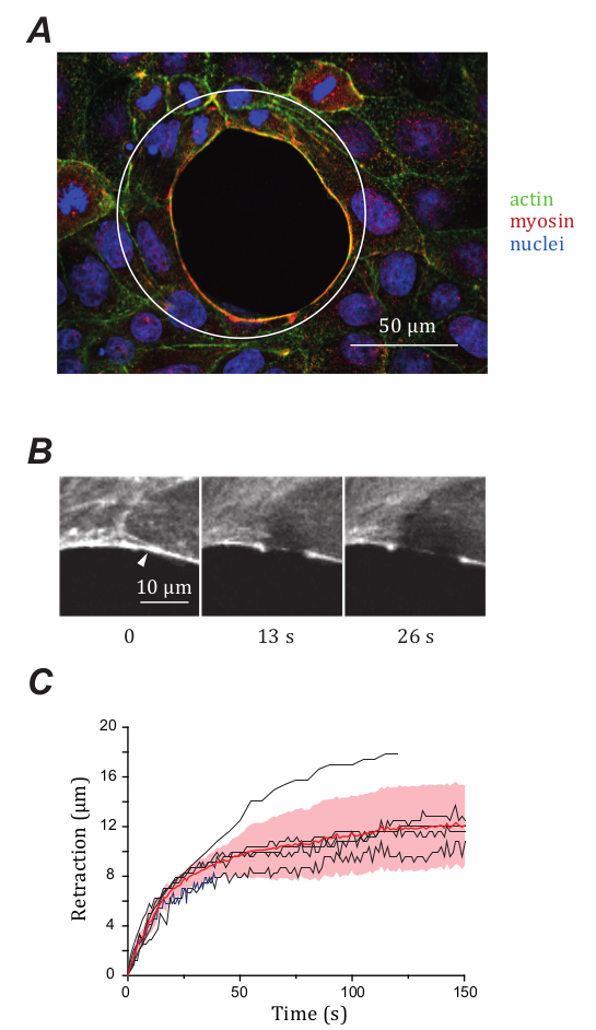
Figure 4: A contractile pluricellular actomyosin cable localizes at the border of the monolayer. A Colocalisation of actin and myosin at the free edge of the closing epithelium. The white circle is the underlying domain. B Ablation of the cable (ablation point is figured by the white triangle) at t=0 and its subsequent retraction. C Dynamics of retraction of cables on several wounds. The red line is the average retraction, the pink area is the standard deviation.

Methods

Preparation of the patterns

Non-adherent domains of varying radii were micropatterned onto cleaned glass cover slips. The glass slides were first uniformly treated by a surface treatment of polyacrylamide and polyethyleneglycol (PEG) on which cells do not adhere (18, 19, 38). Domains whose radii were between $5$ and $75\,\mu$m with a $0.5\,\mu$m increment were defined by photolithography directly on the coating in such a way that it remained protected by the photoresist (S1813, Microchem, Westborough, MA) at the desired location of the non-adhesive domains (19). Using the photoresist as an etching mask, the PEG coating was removed in the photoresist-free areas with an air plasma (Harrick plasma cleaner), revealing the underlying glass. The resist was then dissolved leading to PEG-coated domains surrounded by a clean glass surface. The surface treatment was stable for weeks in biological buffers (19).

Cell culture

MDCK cells (39) were cultured in Dulbecco’s modified Eagle’s medium supplemented with $10\,\%$ FBS (Sigma), $2$ mM L-glutamin solution (Gibco) and $1\,\%$ antibiotic solution (penicillin ($10,000$ units/mL), streptomycin ($10$ mg/mL)). Cells were seeded and maintained at $37^{\circ}$C, $5\,\%$CO2 and $90\,\%$ humidity throughout the experiments. We also used MDCK LifeAct cells (3) for ablation experiments (these clones were cultured in presence of geneticin ($400\,\mu$g/mL)).

Blebbistatin (Sigma) was used at a concentration of $50\,\mu$M. Experiments were started in the absence of the drug. At confluence, a fraction of the supernatant was pumped out, mixed with the drug and re-injected into the well.

Low-calcium medium (calcium-free DMEM, fetal bovine serum $10\,\%$, Penstrep $1\,\%$, $50$ mM calcium) was used to reduce cell-cell adhesion. Experiments were started in regular DMEM and the buffer was changed to low-calcium DMEM at confluence.

Microscopy and data analysis

The bottoms of Petri dishes or 6-well plates were replaced with patterned glass slides. Cells were imaged in phase contrast on an Olympus IX71 inverted microscope equipped with temperature, CO2 and humidity regulation (LIS), a motorized stage for multipositioning (Prior) and a Retiga 4000R camera (QImaging). Unless otherwise specified, a $10\times$ objective was used and images were acquired every $30$ min. Displacements and image acquisition were computer-controlled with Metamorph (Molecular Devices).

Fixed fluorescently marked cells were observed under an upright Imager Z2 spinning disk microscope (Zeiss, Oberkochen, Germany) equipped with a CoolSnapHQ2 camera (Photometrics, Tuscon, AZ) and a $63\times$ water immersion objective. All acquisitions were controlled using MetaMorph software (Molecular Devices, Sunnyvale, CA).

Images were processed with the ImageJ software or with Matlab (MathWorks, Natick, MA) routines. Further analysis was occasionally performed on Origin (OriginLab, Northampton, MA).

Unless otherwise specified, fractions were computed from at least 100 domains for each size measured over at least 4 distinct experiments.

Laser ablations

Photoablation experiments were performed on an LSM 710 NLO (Zeiss) microscope equipped with a two-photon MaiTai laser and a $40\times$ oil immersion objective. The two-photon laser was used at $85\,\%$ power and at a wavelength of $890$ nm.

Immunoflurocescence

Cells were fixed in $4\,\%$ PFA, permeabilized in $0.1\,\%$ Triton X-100 and blocked in $10\,\%$ FBS in PBS. Vinculin labeling was performed with a mouse monoclonal anti-vinculin antibody (Sigma, 1:500) and Paxillin labeling was performed with a mouse anti-paxillin antibody (Sigma, 1:500) both followed by Alexa 488 donkey anti-mouse (Life Technologies, 1:500). Actin was labeled using Alexa 546 phalloidin (Life Technologies, 1:1000). Myosin was labeled with rabbit anti-phospho myosin light chain (Ozyme, Saint Quentin en Yvelines, France, 1:100) followed by Alexa 488 chicken anti-rabbit (Life Technologies, 1:1000). Hoescht 33342 (Sigma, 1:10000) was used to mark the nuclei.

References

1. Ray HJ, Niswander L (2012) Mechanisms of tissue fusion during development. Development 139:1701-11.

2. Martin P (1997) Wound healing–aiming for perfect skin regeneration. Science 276:75.

3. Cochet-Escartin O, Ranft J, Silberzan P, Marcq P (2014) Border forces and friction control epithelial closure dynamics. Biophys J 106:65-73.

4. Anon E et al. (2012) Cell crawling mediates collective cell migration to close undamaged epithelial gaps. Proc Natl Acad Sci U S A 109:10891-6.

5. Brugués A et al. (2014) Forces driving epithelial wound healing. Nat Phys 10:683.

6. Reffay M et al. (2014) Interplay of RhoA and mechanical forces in collective cell migration driven by leader cells. Nat Cell Biol 16:217.

7. Abreu-Blanco MT, Verboon JM, Liu R, Watts JJ, Parkhurst SM (2012) Drosophila embryos close epithelial wounds using a combination of cellular protrusions and an actomyosin purse string. J Cell Sci 125:5984-97.

8. Copp AJ, Brook FA, Estibeiro JP, Shum AS, Cockroft DL (1990) The embryonic development of mammalian neural tube defects. Prog Neurobiol 35:363-403.

9. Bement WM, Mandato C, Kirsch MN (1999) Wound-induced assembly and closure of an actomyosin purse string in Xenopus oocytes. Curr Biol 9:579-87.

10. Kiehart DP (1999) Wound healing: The power of the purse string. Curr Biol 9:R602-605.

11. Jacinto A, Martinez-Arias A, Martin P (2001) Mechanisms of epithelial fusion and repair. Nat Cell Biol 3:E117-E123.

12. Hutson MS et al. (2003) Forces for morphogenesis investigated with laser microsurgery and quantitative modeling. Science 300:145-9.

13. Friedl P, Locker J, Sahai E, Segall JE (2012) Classifying collective cancer cell invasion. Nat Cell Biol 14:777-783.

14. Curtis A, Varde M (1964) Control of cell behavior: topological factors. J Natl Cancer Inst 33:15-26.

15. Vedula SRK et al. (2014) Epithelial bridges maintain tissue integrity during collective cell migration. Nat Mater 13:87-96.

16. Gautrot JE et al. (2012) Mimicking normal tissue architecture and perturbation in cancer with engineered micro-epidermis. Biomaterials 33:5221-9.

17. Vedula SRK et al. (2015) Mechanics of epithelial closure over non- adherent environments. Nat Commun 6:6111.

18. Tourovskaia A, Figueroa-Masot X, Folch A (2006) Long-term microfluidic cultures of myotube microarrays for high-throughput focal stimulation. Nat Protoc 1:1092-104.

19. Deforet M, Hakim V, Yevick HG, Duclos G, Silberzan P (2014) Emergence of collective modes and tri-dimensional structures from epithelial confinement. Nat Commun 5:3747.

20. Underhill GH, Galie P, Chen CS, Bhatia SN (2012) Bioengineering methods for analysis of cells in vitro. Annu Rev Cell Dev Biol 28:385-410.

21. Harris AR et al. (2012) Characterizing the mechanics of cultured cell monolayers. Proc Natl Acad Sci U S A 109:16449-54.

22. Petitjean L et al. (2010) Velocity fields in a collectively migrating epithelium. Biophys J 98:1790-800.

23. Geiger B, Spatz JP, Bershadsky AD (2009) Environmental sensing through focal adhesions. Nat Rev Mol Cell Biol 10:21-33.

24. Bischofs IB, Safran S, Schwarz US (2004) Elastic interactions of active cells with soft materials. Phys Rev E 69:1-17.

25. Guthardt Torres P, Bischofs IB, Schwarz US (2012) Contractile network models for adherent cells. Phys Rev E 85:1-13.

26. Rossier OM et al. (2010) Force generated by actomyosin contraction builds bridges between adhesive contacts. EMBO J 29:1055-68.

27. Kim JH et al. (2013) Propulsion and navigation within the advancing monolayer sheet. Nat Mater 12:856-863.

28. Bar-Ziv R, Tlusty T, Moses E, Safran S, Bershadsky AD (1999) Pearling in cells: A clue to understanding cell shape. Proc Natl Acad Sci U S A 96:10140-10145.

29. Bischofs IB, Klein F, Lehnert D, Bastmeyer M, Schwarz US (2008) Filamentous network mechanics and active contractility determine cell and tissue shape. Biophys J 95:3488-96.

30. Gardiner WC (2004) Handbook of stochastic methods for physics, chemistry and the natural sciences (Springer-Verlag, Berlin).

31. Bevington PR, Robinson DK (1969) Data reduction and error analysis for the physical sciences (McGraw-Hill, New York).

32. Kloedel P, Platen E (1999) Numerical simulations of stochastic differential equations (Springer).

33. Yoshinaga N, Marcq P (2012) Contraction of cross-linked actomyosin bundles. Phys Biol 9:046004.

34. Ranft J et al. (2010) Fluidization of tissues by cell division and apoptosis. Proc Natl Acad Sci U S A 107:20863-8.

35. Douezan S, Brochard-Wyart F (2012) Active diffusion-limited aggregation of cells. Soft Matter 8:784.

36. Martin E, Behn U, Germano G (2011) First-passage and first-exit times of a Bessel-like stochastic process. Phys Rev E 83:051115.

37. Yevick HG, Duclos G, Bonnet I, Silberzan P (2015) Architecture and migration of an epithelium on a cylindrical wire. Proc Natl Acad Sci 112:5944-5949.

38. Tourovskaia A et al. (2003) Micropatterns of Chemisorbed Cell Adhesion-Repellent Films Using Oxygen Plasma Etching and Elastomeric Masks. Langmuir 19:4754-4764.

39. Bellusci S, Moens G, Thiery J-P, Jouanneau J (1994) A scatter factor- like factor is produced by a metastatic variant of a rat bladder carcinoma cell line. J Cell Sci 107:1277-87.

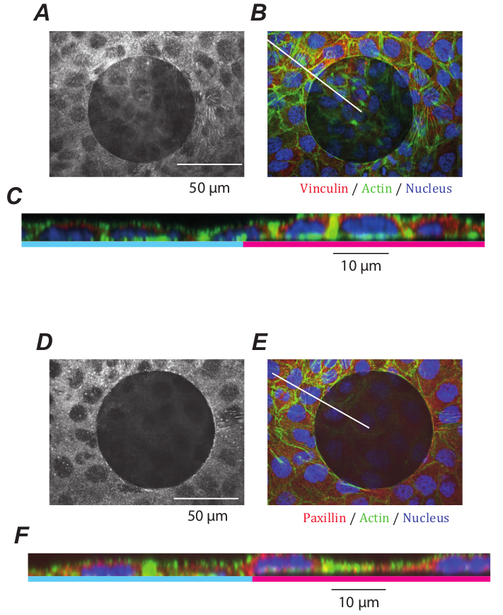
Figure 2: The cells do not develop adhesions with their substrate. A-B and D-E show no significant signal of the adhesion proteins vinculin (A) or paxillin (D) at the basal plane. C,F On the $xz$ sections a thin line void of proteins can be seen over the non-adherent surface (figured in red while the adhering surface is blue). The white lines in panels B and D are the plane of the sections C and F. A-C: $R=41\,\mu$m; D-F: $R=45.5\,\mu$m.

Figure 3: Variability of the trajectories. Individual trajectories are noisy but also define a very broad distribution of closure times. $R=35\,\mu$m.

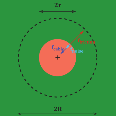
Figure 5: Schematics of the model. Force balance of a line element at the wound margin, for a circular wound of radius $r$. The three lineic force densities depicted are: the tension of the actomyosin cable, a viscous friction force, and a fluctuating force. The initial radius of the non-adhesive patch is $R$. (the cell monolayer is represented in green; the non-adherent surface in red).

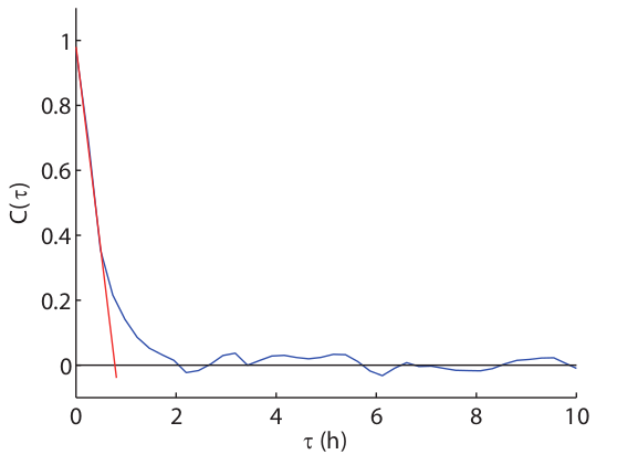
Figure 6: Noise autocorrelation function. We use the Langevin equation (1) to measure the noise term $\eta(t)=\frac{1}{\sqrt{2D}}\,\left(\dot{r}+\frac{\tilde{\gamma}}{r}\right)$ for each trajectory, with the fitted parameter values $\tilde{\gamma}=10\;\mu\mathrm{m^{2}h^{-1}}$ and $D=1.6\;\mu\mathrm{m^{2}h^{-1}}$. The noise autocorrelation function is obtained by ensemble averaging: $C(\tau)=\langle\eta(t)\eta(t+\tau)\rangle$. It decays quickly, with a correlation time of the order of $1$h.

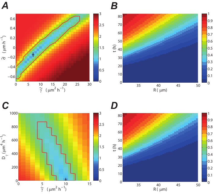
Figure 7: Model robustness. A,B Influence of an epithelial tension. (A) $(\tilde{\gamma},\tilde{\sigma})$ plane of the error landscape at $D=1.5\;\mu\mathrm{m^{2}h^{-1}}$ (logarithmic scale). The cross denotes the optimum, the red contour bounds the confidence region. (B) Optimal closure frequency map (linear scale), computed for $\tilde{\gamma}=7\;\mu\mathrm{m^{2}h^{-1}}$, $D=1.5\;\mu\mathrm{m^{2}h^{-1}}$ and $\tilde{\sigma}=-0.15\;\mu\mathrm{m^{2}h^{-1}}$. C,D Influence of fluctuations of the cable tension. (C) $(\tilde{\gamma},D_{\gamma})$ plane of the error landscape at $D=1.5\;\mu\mathrm{m^{2}h^{-1}}$ (logarithmic scale). The cross denotes the optimum, the red contour bounds the confidence region. (D) Optimal closure frequency map (linear scale), computed for $\tilde{\gamma}=10\;\mu\mathrm{m^{2}h^{-1}}$, $D=1.5\;\mu\mathrm{m^{2}h^{-1}}$ $D_{\gamma}=10\;\mu\mathrm{m^{2}h^{-1}}$.

Supplementary Notes

1 A stochastic description

1.1 A Langevin equation

Wound closure dynamics on a nonadhesive patch is a noisy process, with, e.g., large fluctuations of the closure time $t_{c}$ at a given radius $R$. This observation calls for a stochastic description. Since the wound is approximately invariant by rotation about its center, force balance on a line element at the margin may be expressed as a stochastic equation for the wound radius $r(t)$

$$-\xi\dot{r}+F_{1}(r,t)+F_{2}(r,t)=0$$ (4)

where $F_{1}(r,t)$ and $F_{2}(r,t)$ respectively denote the deterministic and the stochastic component of the lineic force density, and $\xi$ is an effective friction coefficient subsuming all dissipative processes at play. Since ablation experiments show that the circumferential actomyosin cable is under tension, we write

$$F_{1}(r,t)=-\frac{\gamma}{r}$$ (5)

where $\gamma$ denotes the line tension of the contractile cable (see Supp. Fig. 5).

A simple stochastic model of the dynamics may be written as

$$\dot{r}(t)=D_{1}(r,t)+\sqrt{2D_{2}(r,t)}\,\eta(t)$$ (6)

where $D_{1}$ and $D_{2}$ respectively denote the drift and diffusion coefficients, and $\eta(t)$ is a Gaussian white noise with an autocorrelation function $\langle\eta(t)\eta(t^{\prime})\rangle=\delta(t-t^{\prime})$. Dividing the parameter $\gamma$ by the friction coefficient $\xi$ gives a drift coefficient:

$$D_{1}(r,t)=-\frac{\tilde{\gamma}}{r},$$ (7)

with $\tilde{\gamma}=\gamma/\xi$.

Unless explicitly mentioned, we study in the following the stochastic dynamics generated by the Langevin equation

$$\dot{r}(t)=-\frac{\tilde{\gamma}}{r}+\sqrt{2D}\,\eta(t)$$ (8)

with a constant diffusion coefficient $D$

$$D_{2}(r,t)=D$$ (9)

We observe that collective migration always tends to close the cell-free space, which never opens up beyond the area of the non-adhesive patch. The boundary condition at $r=R$ is therefore reflecting. Since closed wounds do not re-open, the boundary condition at $r=0$ is absorbing. In numerical simulations of the Langevin equation, using a finite time step $h$ [32], the boundary conditions are implemented as follows:

• absorbing condition at $r=0$: the simulation stops whenever the radius becomes negative $r(t+h)<0$;

• reflecting condition at $r=R$: a radius larger than $R$, $r(t+h)>R$ is replaced by a radius smaller than $R$, $2R-r(t+h)<R$.

1.2 A Fokker-Planck equation

Eq. (6) is equivalent to an evolution equation for the transition probability distribution function $p(r,t\mid R,0)$ between a radius $R$ at the initial time $0$ and a radius $r$ at time $t$ [30]. It is convenient to write the backward Fokker-Planck equation for $p(r,t\mid R,0)$:

$$\frac{\partial{}}{\partial{t}}p(r,t\mid R,0)=D_{1}(r,t)\,\frac{\partial{}}{\partial{R}}p(r,t\mid R,0)+D_{2}(r,t)\,\frac{\partial^{2}{}}{\partial{R^{2}}}p(r,t\mid R,0)$$ (10)

The probability $f(R,t)$ that a patch with radius $R$ is closed at time $t$, or closure frequency, reads

$$f(R,t)=\mathrm{Prob}(t_{c}(R)\leq t)=1-\int_{0}^{R}p(r,t\mid R,0)\,\mathrm{d}r$$ (11)

Integrating (10) over $r$, we obtain the evolution equation for the closure frequency

$$\frac{\partial{}}{\partial{t}}f(R,t)=D_{1}(R,t)\,\frac{\partial{}}{\partial{R}}f(R,t)+D_{2}(R,t)\,\frac{\partial^{2}{}}{\partial{R^{2}}}f(R,t)$$ (12)

Since wounds are initially open, the initial condition is $f(R_{\mathrm{i}},0)=0$ for an initial radius $R=R_{\mathrm{i}}$. For all time $t$, we naturally impose $f(0,t)=1$ at $R=0$, and the reflecting boundary condition at $R_{\mathrm{i}}$ reads $\frac{\partial{f}}{\partial{R}}(R_{\mathrm{i}},t)=0$ [30].

Using this set of initial and boundary conditions, the numerical resolution of Eq. (12) is performed with the function pdepe of Matlab. For a given set of model parameters, Eq. (12) is solved on the interval $R\in[0,R_{\mathrm{i}}]$. The value at $R_{\mathrm{i}}$, $f_{\mathrm{th}}(R_{\mathrm{i}},t)=f(R=R_{\mathrm{i}},t)$ can then be compared with the experimentally measured fraction $f_{\mathrm{exp}}(R_{\mathrm{i}},t)$ of wounds of initial radius $R_{\mathrm{i}}$ closed at time $t$.

From Eq. (11), $f(R,t)$ is also the cumulated distribution function of closure times. As a consequence, the distribution function $P(t_{\mathrm{c}}\mid R)$ of the closure times $t_{\mathrm{c}}$ of patches of radius $R$ is obtained by differentiating $f$ with respect to time:

$$P(t_{\mathrm{c}}\mid R)=\frac{\partial{f}}{\partial{t}}(R,t_{\mathrm{c}})$$ (13)

2 Parameter fitting and model selection

2.1 A least-squares method

In this section, the theoretical closure frequencies $f_{\mathrm{th}}(R,t\mid\tilde{\gamma},D)$ are computed numerically for a given set of parameter values $(\tilde{\gamma},D)$. Initial and boundary conditions for the evolution equation

$$\frac{\partial{}}{\partial{t}}f(R,t)=-\frac{\tilde{\gamma}}{R}\,\frac{\partial{}}{\partial{R}}f(R,t)+D\,\frac{\partial^{2}{}}{\partial{R^{2}}}f(R,t)$$ (14)

are given in Sec. 1.2. Varying $(R,t)$ at fixed $(\tilde{\gamma},D)$, we calculate the mean square standardized error $E^{2}(\tilde{\gamma},D)$ between theoretical frequencies and experimental fractions [31]:

$$E^{2}(\tilde{\gamma},D)=\frac{1}{N}\,\sum_{R,t}\frac{\left(f_{\mathrm{th}}(R,t\mid\tilde{\gamma},D)-f_{\mathrm{exp}}(R,t)\right)^{2}}{\sigma_{f_{\mathrm{exp}}}^{2}(R,t)}$$ (15)

where $N$ is the total number of data points, and $\sigma_{f_{\mathrm{exp}}}^{2}(R,t)$ is the variance of the fraction of patches of radius $R$ closed at time $t$, as measured over $N_{\mathrm{exp}}(R)$ experiments:

$$\sigma_{f_{\mathrm{exp}}}^{2}(R,t)=\frac{f_{exp}(R,t)\left(1-f_{exp}(R,t)\right)}{N_{\mathrm{exp}}(R)}$$ (16)

The experimental fractions $f_{\mathrm{exp}}(R,t)$ are measured from a total of $6625$ patches, with radii ranging from $31$ to $49.5\,\mu$m with a $0.5\,\mu$m step, over a total duration $T=83$h, and with a time resolution $\Delta t=1$h. In practice, we define $\mathrm{N_{R}}=13$ bins of width $\Delta R=1.5\,\mu$m and $\mathrm{N_{t}=84}$ time points per radius, so that $N=N_{R}\,N_{t}=1092$.

The error landscape is shown in Fig. 3C. The minimum of the mean square error is achieved for

$$\tilde{\gamma}_{\mathrm{min}} = 10\;\mu\mathrm{m^{2}h^{-1}}$$ (17)

$$D_{\mathrm{min}} = 1.6\;\mu\mathrm{m^{2}h^{-1}}$$ (18)

corresponding to a minimal mean square error value

$$E^{2}_{\mathrm{min}}=\mathrm{min}_{\tilde{\gamma},D}\,E^{2}(\tilde{\gamma},D)=E^{2}(\tilde{\gamma}=\tilde{\gamma}_{\mathrm{min}},D=D_{\mathrm{min}})\simeq 7.6$$ (19)

at the bottom of a well-defined single well. The optimal parameter values (17-18) yield the best agreement with experimental data (compare Figs. 3A and 3B).

At a given radius $R$ and time $t$, the $95\,\%$ confidence interval of the optimal theoretical frequency $f_{\mathrm{th}}^{\mathrm{min}}=f_{\mathrm{th}}(R,t\mid\tilde{\gamma}_{\mathrm{min}},D_{\mathrm{min}})$ reads $[f_{\mathrm{th}}^{\mathrm{min}}-1.96\,\sigma_{f_{\mathrm{exp}}},\;f_{\mathrm{th}}^{\mathrm{min}}+1.96\,\sigma_{f_{\mathrm{exp}}}]$, where $\sigma_{f_{\mathrm{exp}}}$ is a proxy for the standard deviation of $f_{\mathrm{th}}^{\mathrm{min}}$. Substituting the upper bound of the confidence interval for $f_{\mathrm{th}}^{\mathrm{min}}$ into Eq. (15) yields an upper bound of the mean square error

$$E^{2}_{+} = \frac{1}{N}\,\sum_{R,t}\frac{\left(f_{\mathrm{th}}^{\mathrm{min}}(R,t)+1.96*\sigma_{f_{\mathrm{exp}}}(R,t)-f_{\mathrm{exp}}(R,t)\right)^{2}}{\sigma_{f_{\mathrm{exp}}}^{2}(R,t)}$$ (20)

$$= E^{2}_{\mathrm{min}}+2*1.96*\frac{1}{N}\,\sum_{R,t}\frac{f_{\mathrm{th}}^{\mathrm{min}}(R,t)-f_{\mathrm{exp}}(R,t)}{\sigma_{f_{\mathrm{exp}}}(R,t)}+1.96^{2}$$ (21)

We define the confidence region for the parameters $(\tilde{\gamma},D)$ by the domain within the level contour $E^{2}(\tilde{\gamma},D)=E^{2}_{+}=15.8$, see Fig. 3C. Conservative estimates of confidence intervals on $\tilde{\gamma}$ and $D$ (in brackets) are finally obtained by inscribing this contour within a rectangle:

$$\tilde{\gamma} = 10\;\mu\mathrm{m^{2}h^{-1}}\quad[6,13]$$ (22)

$$D = 1.6\;\mu\mathrm{m^{2}h^{-1}}\quad[0.5,3.9]$$ (23)

The value of the dimensionless ratio $\frac{D_{2}}{RD_{1}}$ allows to determine whether drift or diffusion dominate the dynamics. Since

$$\left|\frac{D_{2}}{RD_{1}}\right|=\frac{D}{\tilde{\gamma}}=0.16\quad[0.04,0.65]$$ (24)

we conclude that drift dominates, but that diffusion cannot be neglected.

2.2 Influence of an epithelial tension

Since tissues may quite generally be under compression or under tension, we first tested the robustness of our results by taking into account an epithelial tension $\sigma$ of unknown sign. Force balance is modified: a reduced tension coefficient $\tilde{\sigma}=\sigma/\xi$ contributes to the drift coefficient. Following the procedure given in Sec.2.1, here based on the Langevin equation

$$\dot{r}(t)=-\frac{\tilde{\gamma}}{r}+\tilde{\sigma}+\sqrt{2D}\,\eta(t)$$ (25)

the optima and confidence intervals for the three unknown parameters $(\tilde{\gamma},\tilde{\sigma},D)$ are

$$\tilde{\gamma} = 7\,\mu\mathrm{m^{2}h^{-1}}\,[0,26]$$ (26)

$$D = 1.5\,\mu\mathrm{m^{2}h^{-1}}\,[0.4,3.9]$$ (27)

$$\tilde{\sigma} = -0.15\,\mu\mathrm{m\,h^{-1}}\,[-0.65,0.65]$$ (28)

for a minimal value of the error $E^{2}_{\mathrm{min}}=\mathrm{min}_{\tilde{\gamma},\tilde{\sigma},D}\,E^{2}(\tilde{\gamma},\tilde{\sigma},D)=7.2$ (see Supp. Fig. 7A).

Strikingly, zero belongs to the confidence interval for $\tilde{\sigma}$, and the level of agreement between predictions and data is not improved when taking into account the (small, negative) optimal value (28) (compare Supp. Fig. 7AB with Fig. 3AB). Further, the revised estimates (26-27) for $\tilde{\gamma}$ and $D$ are consistent with the previous confidence intervals (22-23). We conclude that the closure fraction data is consistent with the absence of measurable tension in the monolayer ($\sigma=0$). Indeed little to no retraction was observed when performing laser ablation in the monolayer away from the margin.

2.3 Influence of fluctuations of the cable tension

The diffusion coefficient $D$ is proportional to the amplitude of fluctuations of the epithelial tension about its (zero) average value. We also tested the robustness of our results by taking into account possible fluctuations of the the cable tension, of amplitude $D_{\gamma}\geq 0$. Assuming for simplicity that fluctuations in the cable tension and in the epithelial tension are uncorrelated, we express the diffusion $D_{2}(r,t)$ as

$$D_{2}(r,t)=D+\frac{D_{\gamma}}{r^{2}}$$ (29)

and study the modified Langevin equation

$$\dot{r}(t)=-\frac{\tilde{\gamma}}{r}+\sqrt{2\left(D+\frac{D_{\gamma}}{r^{2}}\right)}\,\eta(t)$$ (30)

interpreted according to Ito’s rule. This model leads to the estimates

$$\tilde{\gamma} = 10\,\mu\mathrm{m^{2}.h^{-1}}\,[4,12]$$ (31)

$$D = 1.5\,\mu\mathrm{m^{2}.h^{-1}}\,[0,2.5]$$ (32)

$$D_{\gamma} = 10\,\mu\mathrm{m^{4}.h^{-1}}\,[0,870]$$ (33)

for a minimal value of the error $E^{2}_{\mathrm{min}}=\mathrm{min}_{\tilde{\gamma},D,D_{\gamma}}\,E^{2}(\tilde{\gamma},D,D_{\gamma})=7.5$. We emphasize that: (i) the optimal values in (31-32) are consistent with the confidence intervals (22-23); (ii) a non-zero value of $D_{\gamma}$ (32) has little influence on the level of agreement between theoretical and experimental closure fractions (compare Supp. Figs. 6C-D and Figs. 3A-B).

Taking into account fluctuations of the cable tension allows to define two critical radii:

$$R_{\gamma}^{(1)}=\sqrt{\frac{D_{\gamma}}{D}},\quad\quad R_{\gamma}^{(2)}=\sqrt{\frac{D_{\gamma}}{\tilde{\gamma}}}$$ (34)

Fluctuations of the cable tension dominate fluctuations of the epithelial tension below $R_{\gamma}^{(1)}$, and dominate the deterministic cable tension below $R_{\gamma}^{(2)}$. Using (31-33), we find $R_{\gamma}^{(1)}\simeq 3\,\mu$m and $R_{\gamma}^{(2)}\simeq 1\,\mu$m: this suggests that cable tension fluctuations may dominate the very late stage of the closure process.

Conversely, we find that cable tension fluctuations are negligible except near closure, and conclude by selecting the most parsimonious model, Eq. (8), which we will use in Sec. 3 to define and compute additional quantifiers of closure dynamics.

3 Statistical quantifiers of closure dynamics

3.1 Closure half-time $t_{\nicefrac{{1}}{{2}}}$

We first consider the closure half-time $t_{\nicefrac{{1}}{{2}}}$, defined as the time needed to close half of the wounds for a given initial radius $R$:

$$f(R,t_{\nicefrac{{1}}{{2}}})=\frac{1}{2}.$$ (35)

Experimentally, $t_{\nicefrac{{1}}{{2}}}$ becomes larger than the total duration of the experiment $t_{\nicefrac{{1}}{{2}}}>83$ h above a radius $R=44.5\,\mu\mathrm{m}$. In Fig. 3D, we compare our measurement of the half-closure time up to $R=49.5\,\mu\mathrm{m}$ with the outcome of numerical simulations for the optimal parameters (17-18). Experimental error bars are obtained from the maximum $\mathrm{max\left(t^{+}-t_{\nicefrac{{1}}{{2}}},t_{\nicefrac{{1}}{{2}}}-t^{-}\right)}$ where the times $t^{\pm}$ are defined by $f_{\mathrm{exp}}(\mathrm{R,t}^{\pm})=\frac{1}{2}\left(1\pm\frac{1}{N_{\mathrm{exp}}(R)}\right)$. As expected by comparing Figs. 3A-B, where the same closure fraction data and theoretical frequencies are plotted as a heat map, experimental and theoretical values agree very well in Fig. 3D.

3.2 Distribution of closure times $t_{\mathrm{c}}$

Figs. 2C-E compare experimental and theoretical closure time distributions for radii $R=34$, $40$ and $46\,\mu\mathrm{m}$. Experimental values are computed, within $\Delta R=1.5\,\mu\mathrm{m}$ and binned over time intervals of $\Delta t=12$h, by discrete differentiation of $f_{\mathrm{exp}}$,

$$P_{\mathrm{exp}}(t_{\mathrm{c}}\mid R)=\frac{f_{\mathrm{exp}}(R,t_{\mathrm{c}}+\Delta t)-f_{\mathrm{exp}}(R,t_{\mathrm{c}}-\Delta t)}{2\Delta t}$$ (36)

The error bars in Figs. 2C-E are calculated from (16) according to

$$\Delta P_{\mathrm{exp}}(t_{\mathrm{c}}\mid R)=\left(\frac{\sigma_{f_{\mathrm{exp}}}^{2}(R,t_{\mathrm{c}}+\Delta t)+\sigma_{f_{\mathrm{exp}}}^{2}(R,t_{\mathrm{c}}-\Delta t)}{4\Delta t^{2}}\right)^{\nicefrac{{1}}{{2}}}.$$ (37)

Theoretical frequencies are computed using Eq. (13). We find reasonable agreement within error bars.

3.3 Mean closure time as a mean first-exit time

The mean closure time $\langle t_{\mathrm{c}}(R)\rangle$ is defined as the mean first-exit time to zero starting from an initial radius $r(0)=R$ [30]. We show that it admits a simple analytical expression for the stochastic process defined by the Langevin equation (8) with an absorbing boundary at $r=0$ and a reflecting boundary at $r=R$.

The solution of the differential equation

$$-\frac{\tilde{\gamma}}{x}\,\frac{\mathrm{d}{}}{\mathrm{d}{x}}T_{1}(x)+D\,\frac{\mathrm{d}^{2}{}}{\mathrm{d}{x}^{2}}T_{1}(x)=-1$$ (38)

supplemented with the boundary conditions $T_{1}(x=0)=0$, $\frac{\mathrm{d}{}}{\mathrm{d}{x}}T_{1}(x=R)=0$ reads

$$T_{1}(x)=\frac{1}{\tilde{\gamma}-D}\left(\frac{x^{2}}{2}-\frac{x^{1+\tilde{\gamma}/D}\,R^{1-\tilde{\gamma}/D}}{1+\tilde{\gamma}/D}\right)$$ (39)

This yields the mean closure time as a function of initial radius $\langle t_{\mathrm{c}}(R)\rangle=T_{1}(x=R)$:

$$\langle t_{\mathrm{c}}(R)\rangle=\frac{R^{2}}{2(\tilde{\gamma}+D)}$$ (40)

This prediction is compared to experimental data in Fig. 2F.

In the absence of force fluctuations, Eq. (8) reduces to $\dot{r}(t)=-\frac{\tilde{\gamma}}{r}$, with the solution $r(t)^{2}=R^{2}-2\tilde{\gamma}t$. For a given initial radius, the deterministic closure time reads

$$t_{\mathrm{c}}^{\mathrm{det}}(R)=\frac{R^{2}}{2\tilde{\gamma}}$$ (41)

As a consequence the ratio

$$\frac{t_{\mathrm{c}}^{\mathrm{det}}(R)}{\langle t_{\mathrm{c}}(R)\rangle}=1+\frac{D}{\tilde{\gamma}}$$ (42)

is always larger than unity: in the presence of fluctuations, the mean closure time $\langle t_{\mathrm{c}}(R)\rangle$ is always shorter than the deterministic closure time $t_{\mathrm{c}}^{\mathrm{det}}(R)$.

3.4 Fluctuations of the closure time

Higher moments can be calculated iteratively [30]. In the case of the second moment $\langle t_{\mathrm{c}}^{2}(r)\rangle$, we solve the differential equation:

$$-\frac{\tilde{\gamma}}{x}\,\frac{\mathrm{d}{}}{\mathrm{d}{x}}T_{2}(x)+D\,\frac{\mathrm{d}^{2}{}}{\mathrm{d}{x}^{2}}T_{2}(x)=-2T_{1}(x)$$ (43)

with the boundary conditions $T_{2}(x=0)=0$ and $\frac{\mathrm{d}{}}{\mathrm{d}{x}}T_{2}(x=R)=0$, and expression (39). The second moment $\langle t_{\mathrm{c}}^{2}(R)\rangle=T_{2}(x=R)$ reads

$$\langle t_{\mathrm{c}}^{2}(R)\rangle=\frac{5+\tilde{\gamma}/D}{(3+\tilde{\gamma}/D)\,(1+\tilde{\gamma}/D)^{2}}\,\frac{R^{4}}{4D^{2}}$$ (44)

The variance simplifies to

$$\sigma^{2}_{t_{\mathrm{c}}}(R)=\langle t_{\mathrm{c}}^{2}(R)\rangle-\langle t_{\mathrm{c}}(R)\rangle^{2}=\frac{2D}{3D+\tilde{\gamma}}\,\langle t_{\mathrm{c}}(R)\rangle^{2}$$ (45)

and the coefficient of variation of the closure time, defined as the ratio of the standard deviation to the mean value, is a constant

$$\frac{\sigma_{t_{\mathrm{c}}}({R})}{\langle t_{\mathrm{c}}(R)\rangle}=\left(\frac{2D}{3D+\tilde{\gamma}}\right)^{\frac{1}{2}}$$ (46)

This prediction is compared to experimental data in Fig. 2G.

4 Initial mean square deviation

In order to explain the diffusive behavior of the mean square deviation observed at short time (See Fig. 2I) we define

$$Y(t)=\frac{r(0)-r(t)}{\sqrt{2D}}$$ (47)

and obtain by substitution in (8), the Langevin equation for $Y(t)$:

$$\dot{Y}=\tilde{D_{1}}+\eta(t)$$ (48)

with a drift coefficient $\tilde{D}_{1}=\frac{\tilde{\gamma}}{r\sqrt{2D}}$. The distribution $p_{o}(Y,t)=p(Y,t\mid 0,0)$ obeys the (forward) Fokker-Planck equation

$$\frac{\partial{}}{\partial{t}}p_{o}(Y,t)=-\frac{\partial{}}{\partial{Y}}\left(\tilde{D_{1}}\,p_{o}(Y,t)\right)+\frac{1}{2}\frac{\partial^{2}{}}{\partial{Y^{2}}}p_{o}(Y,t).$$ (49)

Introducing the scaling variable

$$Z=\frac{Y}{\sqrt{t}}$$ (50)

and assuming that $p_{o}(Y,t)=\frac{1}{\sqrt{t}}\,G(Z)$, Eq. (49) becomes

$$\frac{\mathrm{d}^{2}{G}}{\mathrm{d}{Z}^{2}}+Z\,\frac{\mathrm{d}{G}}{\mathrm{d}{Z}}+G=2\,\sqrt{t}\,\frac{\mathrm{d}}{\mathrm{d}Z}[\tilde{D}_{1}\,G]$$ (51)

The scaling Ansatz (50) is thus valid in the limit

$$2\sqrt{t}\,\tilde{D}_{1}\ll Z$$ (52)

where the differential equation obeyed by $G(Z)$ simplifies to

$$\frac{\mathrm{d}^{2}{G}}{\mathrm{d}{Z}^{2}}+Z\,\frac{\mathrm{d}{G}}{\mathrm{d}{Z}}+Z=0$$ (53)

With the boundary condition $\lim_{Z\to\infty}G(Z)=0$, the normalized solution of Eq. (53) is $G(Z)=\sqrt{\frac{2}{\pi}}\,e^{-Z^{2}/2}$. Given the second moment of $Z$

$$\langle Z^{2}\rangle=\intop_{0}^{+\infty}Z^{2}\,G(Z)\,\mathrm{d}Z=1$$ (54)

we obtain

$$\langle(r(0)-r(t))^{2}\rangle=2D\,\langle Y^{2}\rangle=2D\,\langle Z^{2}\rangle\,t=2D\,t$$ (55)

as expected for simple diffusion.

Since the scaling variable is typically close to $Z\sim 1$ according to Eq. (54), condition (52) amounts to $t\ll\frac{D}{2}(\frac{r}{\tilde{\gamma}})^{2}$. During the early stage of closure, we expect that $r(t)\simeq r(0)$, and for $30\leq r(0)\leq 50\,\mu$m, using the numerical values (17-18) of $\tilde{\gamma}$ and $D$, the above inequality will be respected when $t\ll 7$ h. Fig. 2I confirms that the approximate scaling solution deriving from $G(Z)$ is indeed relevant for $t<2$h.

Note that the scaling (55) does not depend on a specific functional form of the drift $D_{1}(r,t)$, and remains valid for the stochastic process defined in Sec. 2.2 with a non-zero epithelial tension $\sigma$, although in a range (52) that depends on the drift coefficient.

When the diffusion coefficient $D_{2}(r,t)$ depends on $r$ as in Sec. 2.3, we checked that the same diffusive scaling also holds for short time $t$ and small deviations $r(0)-r(t)$: the $r$-dependence of $D_{2}$ can be transformed away by an appropriate definition of $Y$ that generalizes (47). However, the factor $2D$ in Eq. (55) is then replaced by a coefficient that depends upon the experimental distribution of radii.