Geometrical constraint on curvature with BAO experiments
Abstract
The spatial curvature ( or ) is one of the most fundamental parameters of an isotropic and homogeneous universe and has a close link to the physics of the early Universe. Combining the radial and angular diameter distances measured via the baryon acoustic oscillation (BAO) experiments allows us to unambiguously constrain the curvature. The method is primarily based on the metric theory, but is less sensitive to the theory of structure formation other than the existence of the BAO scale and is free of any model of dark energy. In this paper, we estimate a best achievable accuracy of constraining the curvature with the BAO experiments. We show that an all-sky, cosmic-variance-limited galaxy survey covering the Universe up to enables a precise determination of the curvature to an accuracy of . When we assume a model of dark energy – either the cosmological constant or the model – it can achieve a precision of . These forecasts require a high sampling density of galaxies, and are degraded by up to a factor of a few for a survey with a finite number density of .
pacs:
98.80.-k,95.36.+x,95.75.-z,98.65.DxI Introduction
The curvature of the Universe (hereafter denoted as or ) is one of the most fundamental quantities in an isotropic and homogeneous universe in the context of general relativity (GR) (Weinberg, 1972). The curvature also has a close connection to the physics of the early Universe. An inflationary universe scenario predicts that the “apparent” curvature, which we can infer from an observable universe, should appear to be close to a flat geometry (), even if the exact value is nonzero (Guth, 1981; Sato, 1981). If the Universe arose from the decay of a false vacuum via quantum tunneling, it leads to an open geometry ( or ) (Coleman and de Luccia, 1980; Gott, 1982; Bucher et al., 1995; Linde, 1995; Yamamoto et al., 1995). In particular, if the Universe began with “large-field inflation” (Lyth, 1997) – which predicts that the primordial gravitational wave is as large as can be observed in the cosmic microwave background (CMB) anisotropies – or if the universe began with “just enough inflation” in a landscape or multiverse picture, the curvature can be large enough to be measurable – (Weinberg, 1989; Guth and Nomura, 2012; Kleban and Schillo, 2012; Freivogel et al., 2014; Bousso et al., 2014). Further, an addition of the super-curvature perturbation in an open-inflation scenario might resolve the large-scale CMB anomalies (Liddle and Cortês, 2013; Kanno et al., 2013; White et al., 2014). On the other hand, if a closed curvature ( or ) is found, it gives rise to a challenge for the inflationary scenario: the Universe needs to emerge from a specific initial condition of closed curvature (Hartle and Hawking, 1983; Linde, 1995). Thus it is important to constrain the curvature from cosmological observations in order to obtain a clue to the physics of the early universe (also see Ref. Weinberg et al., 2013, for a thorough review of various cosmological probes).
Observations of the CMB have led to the precise measurement of the angular diameter distance to the last scattering surface, preferring a flat geometry as expected in an inflationary scenario (e.g., Komatsu et al., 2011; Planck Collaboration et al., 2015). However, the constraint rests on the use of the standard cosmological model such as the cosmological constant, cold-dark-matter dominated model (CDM model), based on GR and the nearly adiabatic initial conditions. If the assumptions are relaxed – for instance, if a generalized model of dark energy is employed – the CMB constraint on the curvature is largely degraded (Ichikawa et al., 2006). The baryonic acoustic oscillation (BAO) provides us with an alternative, powerful geometrical probe, allowing one to constrain the cosmological distances via measurements of the galaxy clustering pattern in redshift and angular directions, respectively (Seo and Eisenstein, 2003; Hu and Haiman, 2003; Eisenstein et al., 2005; Percival et al., 2007). The BAO experiments are shown to be robust against various astrophysical systematic effects such as the galaxy bias uncertainty (Eisenstein et al., 2007; Seo and Eisenstein, 2007). The current state-of-the-art measurements were done using the Sloan Digital Sky Survey III Baryon Oscillation Spectroscopic Survey (Anderson et al., 2012, 2014; Aubourg et al., 2014), achieving a percent precision of the distance measurement at . Various wide-area spectroscopic galaxy surveys are planned that aim to achieve precise BAO measurements up to higher redshifts: the Subaru Prime Focus Spectrograph (PFS) (Takada et al., 2014), the Dark Energy Spectrograph Instrument (DESI) (Levi et al., 2013), the ESA Euclid satellite mission 111http://sci.esa.int/euclid/, and the NASA WFIRST mission (Spergel et al., 2015).
The BAO method is unique in that it can constrain the radial (more exactly the Hubble expansion rate) distance as well as the angular diameter distance at the redshift of the galaxy survey, while other geometrical probes such as supernovae and gravitational lensing can probe the luminosity or angular distances (and not the radial distance). The relation between the radial and angular diameter distances is purely geometrical and specified by the curvature; if the Universe has a nonzero curvature, the two distances differ. The relation holds for any theory of gravity or dark energy, and rests on the metric theory of a homogeneous and isotropic space, which is a maximally symmetric spacetime described by the Friedmann-Robertson-Walker (FRW) metric (Weinberg, 1972). Hence the purpose of this paper is to estimate the fundamental accuracy of estimating the curvature parameter with the BAO experiments (see Refs. Knox, 2006; Bernstein, 2006, for the previous works based on the similar motivation). To do this, we will assume a cosmic-variance-limited galaxy survey, namely full-sky coverage and a sufficiently high number of density of sampled galaxies.
The structure of this paper is as follows. In Sec. II we discuss the methodology based on the Fisher matrix information formalism, and briefly review the BAO method. In Sec. III we show the main results. Section IV is devoted to discussion. Unless stated otherwise, we will adopt as fiducial model a flat CDM cosmology with , and the Hubble parameter .
II Geometrical estimation of the curvature with BAO distances
II.1 Cosmological distances
We assume that the Universe is statistically isotopic and homogeneous. The spacetime structure of such an universe is described by the FRW metric (Weinberg, 1972). With the metric theory, solving the light propagation in an expanding universe yields a relation between cosmological distances and redshift. The comoving radial distance is given in terms of the integral of the Hubble expansion rate:
| (1) |
where the Hubble expansion rate is given by the time derivative of the scale factor as , and is the redshift, given as where we employed the convention today. The metric theory also gives a geometrical relation between the radial and angular diameter distances:
| (2) |
The different equations are for different geometries of the Universe; open, flat and close geometries, respectively. The curvature is in units of . The CMB experiments (e.g., Ref. Komatsu et al., 2011) give stringent constraints on the curvature, implying , where is the curvature parameter and is the Hubble radius today. Note that throughout this paper we use the comoving angular diameter distance, rather than the physical distance, and the two are related as . For redshifts relevant for galaxy surveys, where holds, Eq. (2) can be expanded around , yielding the approximation
| (3) |
Both and are observables of the BAO experiments for each redshift slice. In the following we will use the above equation to estimate the accuracy of estimating the curvature from BAO information without making many assumption about the theory of structure formation (other than the existence of the BAO scale in the distribution of galaxies) or any model of dark energy.
II.2 Estimator of the curvature and its covariance
Suppose we have the BAO distance measurements in redshift bins, without any gap, over a range of redshift from today up to a maximum redshift : and for ( and ). Here is the comoving Hubble distance: .
The radial distance at the th redshift bin can be estimated by combining the measured Hubble distances over a redshift range (see Eq. 1):
| (4) |
where we have introduced the notations, and . In practice one might want to use a more sophisticated method to estimate to avoid inaccuracy due to the discrete summation, e.g. by assuming that is modeled by a polynomial function of redshift and then estimating the coefficients from fitting of the function to the measured . Here we assume a discrete summation for simplicity.
From Eq. (3), an estimator of the curvature parameter from measurements of the radial and angular diameter distances at the th redshift bin can be given as
| (5) |
Combining the measurements at different redshift bins, we can define the chi-square () to estimate the curvature parameter as
| (6) |
where is the underlying true curvature, treated as a free model parameter in the fitting. denotes the inverse of the covariance matrix defined as
| (7) | |||||
Here the covariance matrices such as describe statistical uncertainties of the BAO observables – the Hubble and angular-diameter distances – given BAO measurements of a galaxy survey:
| (8) |
and so on. Around a flat-geometry universe, where , the covariance matrix is approximated as
| (9) |
II.3 BAO
In this subsection, assuming a hypothetical galaxy survey, we derive the Fisher information matrix of the Hubble and angular diameter distances from the BAO measurements.
The two-point correlation function or the Fourier-transformed counterpart – the power spectrum – is measured as a function of the separation lengths between paired galaxies. In this procedure, the position of each galaxy needs to be inferred from the measured redshift and angular position. Then the separation lengths perpendicular and parallel to the line-of-sight direction from the measured quantities are given as and , where and are the differences between the angular positions and the redshifts of the paired galaxies. For this conversion, we need to assume a reference cosmological model to relate the observables (, ) to the quantities . Thus, the wave numbers are given as
| (11) |
The quantities with the subscript “ref” are the quantities estimated from the observables assuming a “reference” cosmological model, and the quantities without the subscript are the underlying true values. Since the reference cosmological model assumed generally differs from the underlying true cosmology, it causes an apparent distortion in the two-dimensional pattern of galaxy clustering. In principle, this could be measured using only the isotropy of clustering statistics – the so-called Alcock-Paczynski (AP) test Alcock and Paczynski (1979) – but a more robust measurement of both and can be obtained by searching for the “common” BAO scales in the pattern of galaxy clustering, as the standard ruler, in combination with the CMB constraints (Seo and Eisenstein, 2003; Hu and Haiman, 2003; Eisenstein and White, 2004).
We will use the currently standard CDM model as a guidance for the parameter dependence of our constraints and as an effective realistic description of the galaxy clustering. Nevertheless, we would again like to emphasize that the methodology proposed in this paper relies only on an FRW metric theory and the existence of the BAO standard ruler. To be more quantitative, the redshift-space galaxy power spectrum at redshift is given in the linear regime as
| (12) | |||||
where is the linear bias parameter, is the linear redshift-space distortion parameter, defined as Kaiser (1987), is the linear growth rate, is the linear mass power spectrum, and is a constant number and is a parameter to model the residual shot noise. Throughout this paper we assume as the fiducial value in each redshift bin for simplicity. This is a conservative assumption, because most galaxies at higher redshift are very likely to be biased tracers with . When deriving the BAO geometrical constraints we will marginalize over the effect of galaxy bias uncertainty.
To make the parameter forecast, we employ the method developed in Ref. Seo and Eisenstein (2007). In this method, we include the smearing effect of the BAO features due to the bulk flow of galaxies in large-scale structure Matsubara (2008); Taruya et al. (2009); Nishimichi and Taruya (2011). For the BAO survey of multiple redshift bins, the Fisher information matrix of model parameters can be computed as
| (13) |
where is the cosine between the wave vector and the line-of-sight direction, ; is the sum over different redshift bins; is the partial derivative of the galaxy power spectrum (Eq. 12) with respect to the th parameter around the fiducial cosmological model; and the effective survey volume and the Lagrangian displacement fields and to model the smearing effect are given as
| (14) | |||||
| (15) | |||||
| (16) |
Here is the comoving volume of the redshift slice centered at ; the present-day Lagrangian displacement field is for Eisenstein et al. (2007); is the growth rate normalized as ; . The parameter is a parameter to model the reconstruction method of the BAO peaks (see below). In Eq. (13), we take the exponential factor of the smearing effect outside of the derivatives of . This is equivalent to marginalizing over uncertainties in and . The growth rate in or takes into account the smaller smearing effect at higher redshift due to the reduced evolution of large-scale structure. For the parameters, we include the cosmological parameters, the distances in each redshift slice, and the nuisance parameters:
| (17) | |||||
where , and are parameters of the primordial power spectrum, is the amplitude of the primordial curvature perturbation, and and are the spectral tilt and the running spectral index. The set of cosmological parameters determines the shape of the linear power spectrum. For the integration, we set and for all the redshift slices, but the exponential factor in Eq. (13) suppresses the information from the nonlinear scales. The Fisher parameter forecasts depend on the fiducial cosmological model for which we assumed that the model is consistent with the WMAP 7-year data Komatsu et al. (2011). For a galaxy survey of redshift bins, the number of model parameters is in total .
Furthermore, we assume the BAO reconstruction method in Ref. Eisenstein et al. (2007). Since the peculiar velocity field of galaxies in large-scale structure can be inferred from the measured galaxy distribution, the inferred velocity field allows for pulling back each galaxy to its position at an earlier epoch and then reconstructing the galaxy distribution more in the linear regime. As a result, one can correct to some extent the smearing effect in Eq. (13) and sharpen the BAO peaks in the galaxy power spectrum. Padmanabhan et al. (Padmanabhan et al., 2012) implemented this method to the real data, SDSS DR7 LRG catalog, and showed that the reconstruction method can improve the distance error by a factor of 2. The improvement was equivalent to reducing the nonlinear smoothing scale from to , about a factor of 2 reduction in the displacement field. To implement this reconstruction method requires a sufficiently high number density of the sampled galaxies in order to reliably infer the peculiar velocity field from the measured galaxy distribution (see Ref. Anderson et al., 2014, for the latest result). In the Fisher matrix calculation, we used for an implementation of the reconstruction method 222We confirmed that if we assumed we can roughly reproduce the distance measurement accuracy for the SDSS LRGs as found in Ref. Padmanabhan et al. (2012).
The BAO reconstruction has so far been successful in substantially improving the accuracies of both the angular diameter distance and radial Hubble distance estimations (see Ref. Seo et al., 2015, for a recent review). The systematic errors can arise from an imperfect treatment of nonlinear effects such as nonlinearities in the density field and the nonlinear motions of galaxies inside massive halos. A further refinement of the reconstruction method will be required, by using mock catalogs of galaxy surveys, in order to achieve the ultimate precision (e.g., Seo et al., 2015, for such an attempt). A striking advantage of using a higher redshift galaxy survey is that the nonlinear effects are weaker at higher redshifts where large-scale structure evolves less, and it will therefore allow a more robust reconstruction to obtain unbiased measurements of the BAO distances.
In the following forecast, we assume the BAO experiments combined with the CMB constraints expected from the Planck satellite:
| (18) |
where is the Fisher matrix for the CMB measurements. We employ the method in Ref. Takada et al. (2014) to compute the CMB Fisher matrix, where we assume the standard CDM model for the physics prior to recombination that determines the sound horizon scale or the BAO scale.
To estimate the accuracy of the distance estimation with the BAO experiments, we first invert the Fisher matrix and then use the submatrix including elements of the Hubble and angular diameter distances:
| (19) |
where the indices denote the elements including the Hubble and angular diameter distances. The submatrix gives the error covariance matrices of distances, and , after marginalizing over other parameters (6 cosmological parameters and nuisance parameters). Hence the dimension of is . The covariance matrices of and and the cross-covariance matrix are
| (20) |
We use these covariances in Eq. (7) to estimate the accuracy of the curvature estimation.
III Results
III.1 Survey parameters
Here we assume an ideal survey to estimate the fundamental limit of the curvature estimation via the BAO measurements. That is, we assume a galaxy survey with full-sky coverage and a sufficiently high number density of sampled galaxies in each redshift bin up to a given maximum redshift , without any gap. We will study how the curvature determination is degraded when considering a survey with a finite number density of galaxies.
III.2 Forecasts
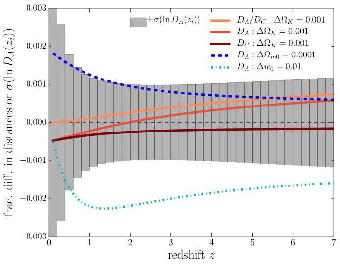
Figure 1 shows the forecasts of the distance measurements with a cosmic-variance-limited survey up to . The shaded region around each redshift bin with width denotes the uncertainty in the angular diameter distance including marginalization (Eq. 20). The accuracy of the Hubble distance is only slightly worse than the error in (at the level of ). As described in Sec. II.3, we include both the BAO feature and the broadband feature of the galaxy power spectrum (the AP test) for the distance forecasts. We confirmed that the distance accuracies are mainly from the BAO features. We should also stress that, once a sufficient number of redshift slices, up to for our setting, are included, the BAO information of the galaxy survey allows a more accurate determination of the sound horizon scale than the Planck prior, which explains why the distance accuracies get saturated at .
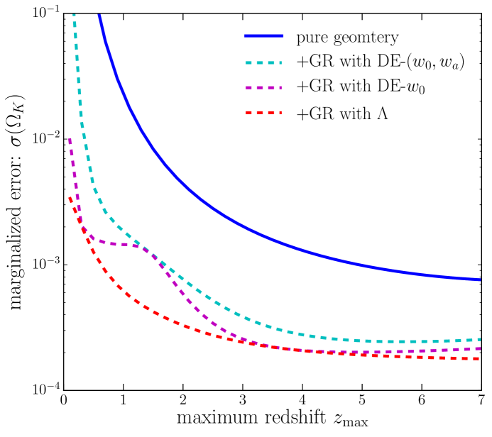
Using the forecasts of the distance measurements, we show in Fig. 2 the expected accuracy of the curvature estimation, . Here we consider a cosmic-variance-limited galaxy survey over a range of redshift and show the forecasts as a function of the maximum redshift . Note that the error is free of the uncertainty in the Hubble parameter , because the uncertainty in is absorbed when estimating the curvature parameter from a combination of the radial and angular distances. The top curve shows the fundamental limit, estimated from Eq. (7), in the sense that the constraint is purely based on the BAO distance measurements and is less sensitive to the theory of structure formation (other than the BAO scale) such as the galaxy bias and is free of any model of dark energy. The accuracy can be better than , if a cosmic-variance-limited survey up to is available. Since the curvature has a relatively larger impact on the expansion history up to higher redshifts than the cosmological constant, adding the BAO distance measurements at higher redshift keeps improving the curvature constraint.
If we employ Einstein gravity (GR), which relates the structure of spacetime to the energy-matter content of the Universe through the Einstein equations, the curvature constraint can be improved, although the constraint is now model-dependent. At redshifts relevant for galaxy surveys, the Hubble expansion rate is given as
| (21) |
Then the Hubble and angular-diameter distances are specified by the density parameters (see Eqs. 1 and 2). However, the nature of dark energy is another mystery of the universe. For comparison, we here employ a phenomenological model of dark energy that is parametrized in terms of its equation-of-state parameters as
| (22) |
where and are parameters and constant in time. In this case, the redshift evolution of dark energy is given as with . We should emphasize that this model acts as a “strong” prior, restricting the degrees of freedom of the dark energy model to a specific model. The redshift dependence of the above dark energy model, around the fiducial cosmological constant model, is different from that of the curvature (), the BAO distance measurements determine the curvature and the dark energy parameters simultaneously. If the dark energy has an (even very small) additive contribution, such as , the contribution leaves a strong degeneracy with the curvature.
Nevertheless it would be useful to estimate the accuracy of the curvature determination from the cosmic-variance-limited BAO measurements when assuming the above dark energy model. To do this, we use the method in Ref. Seo and Eisenstein (2003) to propagate the accuracies of BAO distance measurements into estimations of cosmological parameters. To be more precise, we compute the submatrix of the inverted Fisher matrix of CMB plus the BAO measurements:
| (23) |
The submatrix includes marginalization over other parameters such as galaxy bias (see Eq. 17). Then the elements denoted by include parameters that determine the distances among the set of parameters (Eq. 17), and then we make the parameter forecasts as follows:
| (24) |
The second line denotes a projection of the Fisher matrix onto a new parameter space denoted by . Then the third line denotes a derivation of the marginalized error on the parameter including the curvature and the dark energy parameters.
The dashed curves in Fig. 2 show the marginalized error of the curvature parameter when assuming GR to model the Hubble expansion history and employing the dark energy model, around the fiducial cosmological constant model. By restricting the analysis to a narrower range of dark energy, the curvature constraint can be improved. If assuming the cosmological constant model (the CDM model), the cosmic-variance-limited accuracy can be as high as . The figure shows that the curvature accuracy gets saturated more quickly at , compared to the solid curve without any prior on dark energy. This is for two reasons. First, if the dark energy model is employed, a degeneracy between the curvature and the dark energy parameters can be well broken by adding the BAO measurements in multiple redshifts, where the dark energy around the cosmological constant affects the expansion history only up to . Second, the sound horizon scale can be well determined by adding the BAO measurements up to as we stated above. For these reasons, the BAO measurements at add relatively less information on the curvature when the dark energy models are employed, compared to the case without any prior on dark energy (solid curve).
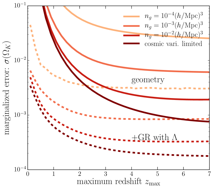
In reality, the accuracy of the curvature determination is degraded by a finite number of sample galaxies for a spectroscopic survey. Figure 3 shows how the curvature estimation is degraded as a function of the number density of galaxies. Here we assume a constant number density of galaxies in each redshift bin for simplicity. The planned galaxy surveys (such as the Subaru PFS, Euclid and WFIRST) are designed so as to satisfy a requirement of at –0.2, corresponding to a number density of (Takada et al., 2014; Spergel et al., 2015). In this case, or 0.0009 for the pure geometry and for the GR+ case, respectively. However, note that these future surveys aim at using mainly emission-line galaxies such as [OII] and/or H emitters as tracers of large-scale structure. The emission-line galaxies are a tiny fraction of imaging galaxies at a depth of mag (less than ). By having a wider wavelength coverage (e.g., up to infrared wavelengths as proposed by the SPHEREx mission Doré et al. (2014)) and/or improving the sensitivity of the spectrograph, a high number density of for a redshift galaxy survey will be feasible in principle. Intergalactic medium surveys, such as Lyman- forests (e.g., Ref. Slosar et al., 2013) or radio intensity mapping (e.g., Ref. Bull et al., 2015) can also be combined with optical and infrared redshift surveys. Hence a (nearly) cosmic-variance-limited BAO survey with is not impossible, although challenging.
IV Discussion
We have estimated the accuracy of the geometrical determination of the spatial curvature from the BAO distance measurements. The BAO is unique in the sense that it allows for a measurement of the radial distance at the redshift of the galaxy survey, while other methods – such as type-Ia supernova and gravitational lensing – measure the luminosity distance which is equivalent to the angular diameter distance. Hence, combining the radial and angular diameter distances allows us to constrain the spatial curvature without making many assumption about the theory of structure formation (other than the BAO scale) such as galaxy bias or any model of dark energy. We showed that an all-sky, cosmic-variance-limited galaxy survey covering up to a high redshift of allows for a curvature determination to an accuracy of . If we assume a simple model of dark energy that is parametrized by two equation-of-state parameters, , it allows for an accuracy of , although the constraint is considered model dependent in this case.
If there is another method of measuring the Hubble expansion rate at high redshift, it might further enable us to improve the curvature constraint based on the method we discussed in this paper. For example, if “red-envelope” galaxies – which have formed their stellar population at higher redshift at – can be used as a cosmic chronometer (as demonstrated in Ref. Stern et al. (2010)), the ages of such red galaxies from detailed spectroscopic observations can be used to estimate the Hubble expansion rate at the galaxy redshift. However, this method still seems to be limited by astrophysical systematic effects; a further careful study needs to be done. The spectroscopic observations of an extremely large-aperture telescope, in combination with the optical frequency comb technique, in principle allow for a precision measurement of the Hubble expansion rate in the high-redshift Universe (e.g., Ref. Liske et al., 2008).
There is an interesting, physical contamination to the estimation of the curvature. A coherent density contrast across a survey region or a local patch in an inhomogeneous universe can appear as a curved universe even if the global geometry is flat Baldauf et al. (2011); Dai et al. (2015). As can be found from Eq. (43) in Ref. Li et al. (2014a), the induced, apparent curvature is expressed as with an prefactor, where is the coherent density contrast. If a local universe is embedded into a coherent underdensity region up to , the comoving survey volume is estimated as for an all-sky survey. The CDM model predicts for the expected rms of the density contrast for the volume, as can be found from Fig. 1 in Ref. Takada and Hu (2013) (also see Ref. Li et al., 2014b). Hence such a negative density contrast could degrade a determination of the global curvature or completely mimic the global curvature, if the true curvature is as small as . However, as stressed in Refs. Takada and Hu (2013); Li et al. (2014b); Takada and Spergel (2013); Schaan et al. (2014) such a coherent density contrast also causes characteristic, scale-dependent modifications in the growth of all small-scale structures (such as weak lensing and cluster abundance) compared to their flat CDM expectations. Hence, although the apparent curvature effects themselves are very intriguing to explore, the effects can in principle be distinguished by combining the geometrical BAO measurements with probes of large-scale structure growth. In addition, even if such a coherent underdensity contrast exists, it would be very difficult (or there would only be an incredibly small chance) to have a situation that we on the Earth are located at the center of such a large-scale void. Hence having a wider-area coverage to explore anisotropic curvature effects on the sky as well as having a larger redshift leverage to explore the void boundary should help distinguish the apparent curvature effects observationally.
Constraining the curvature together with properties of the primordial scalar perturbations and the primordial gravitational wave is an important direction to explore. If a nonzero spatial curvature is found from cosmological observations, it will definitely change our view and understanding of the Universe, so it is worth exploring with any possible means of current or future observational data sets.
Acknowledgements.
We thank Gary Bernstein, Neal Dalal, Chris Hirata, Eiichiro Komatsu, Hitoshi Murayama, Yasunori Nomura, Hirosi Ooguri, and Misao Sasaki for useful discussion. MT is supported by the World Premier International Research Center Initiative (WPI Initiative), MEXT, Japan, by the FIRST program “Subaru Measurements of Images and Redshifts (SuMIRe)”, CSTP, Japan, by a MEXT Grant-in-Aid for Scientific Research on Innovative Areas, “Why does the Universe accelerate? - Exhaustive study and challenge for the future -” (No. 15H05893 and 15K21733), by a Grant-in-Aid for Scientific Research from the JSPS Promotion of Science (No. 23340061 and 26610058), and by the JSPS Program for Advancing Strategic International Networks to Accelerate the Circulation of Talented Researchers. Part of the research described in this paper was carried out at the Jet Propulsion Laboratory, California Institute of Technology, under a contract with the National Aeronautics and Space Administration. OD thanks IPMU for its generous hospitality. This work is also supported in part by the National Science Foundation under Grant No. PHYS-1066293 and the hospitality of the Aspen Center for Physics.References
- Weinberg (1972) S. Weinberg, Gravitation and Cosmology: Principles and Applications of the General Theory of Relativity (1972).
- Guth (1981) A. H. Guth, Phys. Rev. D 23, 347 (1981).
- Sato (1981) K. Sato, Mon. Not. Roy. Astron. Soc. 195, 467 (1981).
- Coleman and de Luccia (1980) S. Coleman and F. de Luccia, Phys. Rev. D 21, 3305 (1980).
- Gott (1982) J. R. Gott, III, Nature (London) 295, 304 (1982).
- Bucher et al. (1995) M. Bucher, A. S. Goldhaber, and N. Turok, Phys. Rev. D 52, 3314 (1995), eprint hep-ph/9411206.
- Linde (1995) A. Linde, Physics Letters B 351, 99 (1995), eprint hep-th/9503097.
- Yamamoto et al. (1995) K. Yamamoto, M. Sasaki, and T. Tanaka, Astrophys. J. 455, 412 (1995), eprint astro-ph/9501109.
- Lyth (1997) D. H. Lyth, Physical Review Letters 78, 1861 (1997), eprint hep-ph/9606387.
- Weinberg (1989) S. Weinberg, Reviews of Modern Physics 61, 1 (1989).
- Guth and Nomura (2012) A. H. Guth and Y. Nomura, ArXiv e-prints (2012), eprint 1203.6876.
- Kleban and Schillo (2012) M. Kleban and M. Schillo, ArXiv e-prints (2012), eprint 1202.5037.
- Freivogel et al. (2014) B. Freivogel, M. Kleban, M. Rodriguez Martinez, and L. Susskind, ArXiv e-prints (2014), eprint 1404.2274.
- Bousso et al. (2014) R. Bousso, D. Harlow, and L. Senatore, ArXiv e-prints (2014), eprint 1404.2278.
- Liddle and Cortês (2013) A. R. Liddle and M. Cortês, Physical Review Letters 111, 111302 (2013), eprint 1306.5698.
- Kanno et al. (2013) S. Kanno, M. Sasaki, and T. Tanaka, Progress of Theoretical and Experimental Physics 2013, 111E01 (2013), eprint 1309.1350.
- White et al. (2014) J. White, Y.-l. Zhang, and M. Sasaki, Phys. Rev. D 90, 083517 (2014), eprint 1407.5816.
- Hartle and Hawking (1983) J. B. Hartle and S. W. Hawking, Phys. Rev. D 28, 2960 (1983).
- Weinberg et al. (2013) D. H. Weinberg, M. J. Mortonson, D. J. Eisenstein, C. Hirata, A. G. Riess, and E. Rozo, Phys. Rep. 530, 87 (2013), eprint 1201.2434.
- Komatsu et al. (2011) E. Komatsu, K. M. Smith, J. Dunkley, C. L. Bennett, B. Gold, G. Hinshaw, N. Jarosik, D. Larson, M. R. Nolta, L. Page, et al., Astrophys. J. Suppl. 192, 18 (2011), eprint 1001.4538.
- Planck Collaboration et al. (2015) Planck Collaboration, P. A. R. Ade, N. Aghanim, M. Arnaud, M. Ashdown, J. Aumont, C. Baccigalupi, A. J. Banday, R. B. Barreiro, J. G. Bartlett, et al., ArXiv e-prints (2015), eprint 1502.01589.
- Ichikawa et al. (2006) K. Ichikawa, M. Kawasaki, T. Sekiguchi, and T. Takahashi, JCAP 12, 5 (2006), eprint arXiv:astro-ph/0605481.
- Seo and Eisenstein (2003) H.-J. Seo and D. J. Eisenstein, Astrophys. J. 598, 720 (2003), eprint arXiv:astro-ph/0307460.
- Hu and Haiman (2003) W. Hu and Z. Haiman, Phys. Rev. D 68, 063004 (2003), eprint arXiv:astro-ph/0306053.
- Eisenstein et al. (2005) D. J. Eisenstein, I. Zehavi, D. W. Hogg, R. Scoccimarro, M. R. Blanton, R. C. Nichol, R. Scranton, H.-J. Seo, M. Tegmark, Z. Zheng, et al., Astrophys. J. 633, 560 (2005), eprint arXiv:astro-ph/0501171.
- Percival et al. (2007) W. J. Percival, S. Cole, D. J. Eisenstein, R. C. Nichol, J. A. Peacock, A. C. Pope, and A. S. Szalay, Mon. Not. Roy. Astron. Soc. 381, 1053 (2007), eprint 0705.3323.
- Eisenstein et al. (2007) D. J. Eisenstein, H.-J. Seo, E. Sirko, and D. N. Spergel, Astrophys. J. 664, 675 (2007), eprint arXiv:astro-ph/0604362.
- Seo and Eisenstein (2007) H.-J. Seo and D. J. Eisenstein, Astrophys. J. 665, 14 (2007), eprint arXiv:astro-ph/0701079.
- Anderson et al. (2012) L. Anderson, E. Aubourg, S. Bailey, D. Bizyaev, M. Blanton, A. S. Bolton, J. Brinkmann, J. R. Brownstein, A. Burden, A. J. Cuesta, et al., ArXiv e-prints (2012), eprint 1203.6594.
- Anderson et al. (2014) L. Anderson, É. Aubourg, S. Bailey, F. Beutler, V. Bhardwaj, M. Blanton, A. S. Bolton, J. Brinkmann, J. R. Brownstein, A. Burden, et al., Mon. Not. Roy. Astron. Soc. 441, 24 (2014), eprint 1312.4877.
- Aubourg et al. (2014) É. Aubourg, S. Bailey, J. E. Bautista, F. Beutler, V. Bhardwaj, D. Bizyaev, M. Blanton, M. Blomqvist, A. S. Bolton, J. Bovy, et al., ArXiv e-prints (2014), eprint 1411.1074.
- Takada et al. (2014) M. Takada, R. S. Ellis, M. Chiba, J. E. Greene, H. Aihara, N. Arimoto, K. Bundy, J. Cohen, O. Doré, G. Graves, et al., Publ. Astron. Soc. Japan 66, R1 (2014), eprint 1206.0737.
- Levi et al. (2013) M. Levi, C. Bebek, T. Beers, R. Blum, R. Cahn, D. Eisenstein, B. Flaugher, K. Honscheid, R. Kron, O. Lahav, et al., ArXiv e-prints (2013), eprint 1308.0847.
- Spergel et al. (2015) D. Spergel, N. Gehrels, C. Baltay, D. Bennett, J. Breckinridge, M. Donahue, A. Dressler, B. S. Gaudi, T. Greene, O. Guyon, et al., ArXiv e-prints (2015), eprint 1503.03757.
- Knox (2006) L. Knox, Phys. Rev. D 73, 023503 (2006), eprint astro-ph/0503405.
- Bernstein (2006) G. Bernstein, Astrophys. J. 637, 598 (2006), eprint astro-ph/0503276.
- Alcock and Paczynski (1979) C. Alcock and B. Paczynski, Nature (London) 281, 358 (1979).
- Eisenstein and White (2004) D. Eisenstein and M. White, Phys. Rev. D 70, 103523 (2004), eprint astro-ph/0407539.
- Kaiser (1987) N. Kaiser, Mon. Not. Roy. Astron. Soc. 227, 1 (1987).
- Matsubara (2008) T. Matsubara, Phys. Rev. D 78, 083519 (2008), eprint 0807.1733.
- Taruya et al. (2009) A. Taruya, T. Nishimichi, S. Saito, and T. Hiramatsu, Phys. Rev. D 80, 123503 (2009), eprint 0906.0507.
- Nishimichi and Taruya (2011) T. Nishimichi and A. Taruya, Phys. Rev. D 84, 043526 (2011), eprint 1106.4562.
- Padmanabhan et al. (2012) N. Padmanabhan, X. Xu, D. J. Eisenstein, R. Scalzo, A. J. Cuesta, K. T. Mehta, and E. Kazin, ArXiv e-prints (2012), eprint 1202.0090.
- Seo et al. (2015) H.-J. Seo, F. Beutler, A. J. Ross, and S. Saito, ArXiv e-prints (2015), eprint 1511.00663.
- Doré et al. (2014) O. Doré, J. Bock, M. Ashby, P. Capak, A. Cooray, R. de Putter, T. Eifler, N. Flagey, Y. Gong, S. Habib, et al., ArXiv e-prints (2014), eprint 1412.4872.
- Slosar et al. (2013) A. Slosar, V. Iršič, D. Kirkby, S. Bailey, N. G. Busca, T. Delubac, J. Rich, É. Aubourg, J. E. Bautista, V. Bhardwaj, et al., JCAP 4, 026 (2013), eprint 1301.3459.
- Bull et al. (2015) P. Bull, S. Camera, A. Raccanelli, C. Blake, P. Ferreira, M. Santos, and D. J. Schwarz, Advancing Astrophysics with the Square Kilometre Array (AASKA14) 24 (2015), eprint 1501.04088.
- Stern et al. (2010) D. Stern, R. Jimenez, L. Verde, M. Kamionkowski, and S. A. Stanford, JCAP 2, 008 (2010), eprint 0907.3149.
- Liske et al. (2008) J. Liske, A. Grazian, E. Vanzella, M. Dessauges, M. Viel, L. Pasquini, M. Haehnelt, S. Cristiani, F. Pepe, G. Avila, et al., Mon. Not. Roy. Astron. Soc. 386, 1192 (2008), eprint 0802.1532.
- Baldauf et al. (2011) T. Baldauf, U. Seljak, L. Senatore, and M. Zaldarriaga, JCAP 1110, 031 (2011), eprint 1106.5507.
- Dai et al. (2015) L. Dai, E. Pajer, and F. Schmidt, JCAP 10, 059 (2015), eprint 1504.00351.
- Li et al. (2014a) Y. Li, W. Hu, and M. Takada, Phys. Rev. D 89, 083519 (2014a), eprint 1401.0385.
- Takada and Hu (2013) M. Takada and W. Hu, Phys. Rev. D 87, 123504 (2013), eprint 1302.6994.
- Li et al. (2014b) Y. Li, W. Hu, and M. Takada, Phys. Rev. D 90, 103530 (2014b), eprint 1408.1081.
- Takada and Spergel (2013) M. Takada and D. N. Spergel, ArXiv e-prints (2013), eprint 1307.4399.
- Schaan et al. (2014) E. Schaan, M. Takada, and D. N. Spergel, ArXiv e-prints (2014), eprint 1406.3330.