Thermonuclear detonations ensuing white dwarf mergers

Abstract

The merger of two white dwarfs (WDs) has for many years not been considered as the favoured model for the progenitor system of type Ia supernovae (SNe Ia). But recent years have seen a change of opinion as a number of studies, both observational and theoretical, have concluded that they should contribute significantly to the observed type Ia supernova rate. In this paper, we study the ignition and propagation of detonation through post-merger remnants and we follow the resulting nucleosynthesis up to the point where a homologous expansion is reached. In our study we cover the entire range of WD masses and compositions. For the emergence of a detonation we study three different setups. The first two are guided by the merger remnants from our earlier simulations (Dan et al., 2014), while for the third one the ignitions were set by placing hotspots with properties determined by spatially resolved calculations taken from the literature. There are some caveats to our approach which we investigate. We carefully compare the nucleosynthetic yields of successful explosions with SN Ia observations. Only three of our models are consistent with all the imposed constraints and potentially lead to a standard type Ia event. The first one, a $0.45\,M_{\odot}\ {\rm helium\ (He)}+0.9\,M_{\odot}$ carbon-oxygen (CO) WD system produces a sub-luminous, SN 1991bg-like event while the other two, a $0.45\,M_{\odot}\ {\rm He}+1.1\,M_{\odot}$ oxygen-neon (ONe) WD system and a $1.05+1.05\,M_{\odot}$ system with two CO WDs, are good candidates for common SNe Ia.

1 Introduction

Thermonuclear supernovae have long been used as cosmological distance indicators. By comparing brightness and redshifts of distant and nearby SNe Ia, it appears that the rate of expansion of the universe is increasing (Riess et al., 1998; Perlmutter et al., 1998). However, their stellar progenitors have so far remained elusive. There is a consensus that the exploding star is a WD made primarily of CO that has a binary companion which donates mass, but the identity of the companion and the exact nature of the explosion mechanism have remained unclear (Maoz et al., 2014). Traditionally, three main scenarios have been proposed to explain the bulk of SNe Ia (for reviews, see Hillebrandt & Niemeyer, 2000; Howell, 2011; Wang & Han, 2012; Postnov & Yungelson, 2014; Maoz et al., 2014). In the so-called “single degenerate” scenario, the CO WD accretes matter from a main sequence, a sub-giant or a red-giant star up to near the Chandrasekhar mass limit, when carbon ignition near the center, followed by a deflagration and later a transition to a detonation, produces a SN Ia-like event (Whelan & Iben, 1973; Nomoto, 1982b). In the “sub-Chandrasekhar” scenario, the CO WD is ignited before it reaches the Chandrasekhar mass (Nomoto, 1982a; Livne, 1990; Woosley & Weaver, 1994; Livne & Arnett, 1995; García-Senz et al., 1999; Fink et al., 2007; Guillochon et al., 2010; Sim et al., 2010; Woosley & Kasen, 2011; Sim et al., 2012; Dan et al., 2012; Moll & Woosley, 2013). In this scenario, a first detonation occurs in the accreted helium material. The resulting shock waves are propagating through the core and may trigger a second detonation close to the interface between the core and the envelope (also known as “edge-lit detonation” model) or close to the core’s centre, where the compressional waves converge (Seitenzahl et al., 2009; Shen & Bildsten, 2014). The second detonation would disrupt the central remnant completely and produce a SN Ia-like event. If only the He shell detonates this could produce a roughly ten times fainter SN Ia, sometimes referred to as SNe “point” Ia (Bildsten et al., 2007; Shen & Bildsten, 2009; Waldman et al., 2011; Holcomb et al., 2013). The “double degenerate” model involves two CO WDs in a close binary system being drawn together as they lose angular momentum by radiating gravitational waves that eventually merges (Iben & Tutukov, 1984; Webbink, 1984). A thermonuclear explosion could be ignited at different stages of the WD-WD binary evolution, either during mass transfer (Guillochon et al., 2010; Pakmor et al., 2013), during the merger (Pakmor et al., 2010; Raskin et al., 2012; Pakmor et al., 2012; Dan et al., 2012; Moll & Woosley, 2013; Sato et al., 2015) or after the merger, in the remnant phase (Dan et al., 2014; Raskin et al., 2014; Kashyap et al., 2015; Sato et al., 2015). Another scenario that could contribute by more than 20% (Tsebrenko & Soker, 2015) to the SN Ia rate is the “core-degenerate” scenario where the WD merges with the core of an asymptotic giant branch star (Livio & Riess, 2003; Kashi & Soker, 2011). These scenarios are meant to explain the bulk of SNe Ia. They may be complemented by rarer channels that trigger thermonuclear explosions in WDs that occur under less common initial conditions. For example, also the compression by the tidal field of a moderately massive black hole may cause a type Ia-like thermonuclear explosion (Luminet & Pichon, 1989; Rosswog et al., 2009b), or, collisions of WDs as they occur in globular cluster cores can produce strong thermonuclear explosions (Rosswog et al., 2009a; Raskin et al., 2009; Kushnir et al., 2013). While the former would typically cause very peculiar events, the latter case produces for the most common WDs around $0.6\,M_{\odot}$ explosions signatures that are similar to typical type Ia events (Rosswog et al., 2009a). Both types of events, however, are most likely too rare to explain the bulk of type Ia events.

The present study will focus on the post-merger remnant phase. The merger remnants show a similar thermodynamic and rotational structure: a cold, isothermal core surrounded by a hot, pressure supported envelope, a rotationally supported disk and a tidal tail (e.g., Guerrero et al., 2004; Yoon et al., 2007; Zhu et al., 2013; Dan et al., 2014). It is inside the hot envelope region of the remnant where the nuclear combustible (helium and, maybe, carbon/oxygen for the most massive WD mergers) may undergo a thermonuclear runaway and a detonation. From the moment when a detonation is ignited, the evolution is very similar to the sub-Chandrasekhar model.

In Dan et al. (2014) we had investigated possible detonations from WD merger remnants by comparing local dynamical and nuclear burning time scales. Dynamical burning, however, is a necessary but not sufficient criterion for the initiation of a detonation (e.g., Holcomb et al., 2013; Shen & Moore, 2014). Therefore, we extend our previous work here with reactive hydrodynamics calculations for a variety of merger remnants. We map nine 3D WD-WD merger remnants representative for the entire WD merger parameter space study of Dan et al. (2014) onto a 2D axisymmetric cylindrical geometry and evolve them with the grid-based code FLASH (Fryxell et al., 2000).

In this study, we expand the previous studies in several ways. Previous multidimensional calculations have started from the initial conditions constructed from spherical symmetric hydrostatic equilibrium models (e.g., Fink et al., 2007; Sim et al., 2012) or from the results of spherically symmetric accretion models (e.g., Moll & Woosley, 2013), while our calculations are starting from realistic WD-WD binary mergers initial conditions taken from the 3D SPH calculations of Dan et al. (2014). Moreover, all previous studies have neglected the angular momentum while in our in models the merger product rotationally supported. If the core detonation is triggered, the rotation together with the presence of the disk can influence the morphology of the ejecta. We carry three sets of tests for each of the nine systems:

• In the first set of tests, we investigate whether the WD remnants could lead to detonations shortly after the restart of the simulations with FLASH.

• For the second set of tests, we manually setup hotspots according with several criteria guided by the 3D SPH simulations. The reason behind this set of tests is that after the mapping onto the grid, the hotspots in the envelope are smoothed out, affecting the thermal evolution. Chemical compositions are also influenced, especially inside chemically mixed regions. For the successful detonations, we also test the impact of different temperature and chemical profiles inside hotspots.

• In a third set of calculations, we asume ad hoc initial conditions in the hotspots following the critical conditions for a spontaneous initiation of a detonation from the spatially resolved 1D calculations of Holcomb et al. (2013); Shen & Moore (2014) for He composition and Röpke et al. (2007); Seitenzahl et al. (2009) for CO.

This paper is organized as follows. In Section 2 we briefly describe our numerical methods and the initial conditions. In Section 3 we present our results in detail, with a focus on the final nucleosynthetic yields and remnant structure for the successfully detonating systems. In Section 4 we summarise our results.

2 Numerical methods

To evolve the WD merger remnants, we are using the Adaptive Mesh Refinement (AMR) FLASH application framework (version 4.2) (http://flash.uchicago.edu) developed by the University of Chicago (Fryxell et al., 2000).

We use the directionally unsplit hydrodynamics solver for the Euler equations for the compressible gas dynamics, the PARAMESH library (MacNeice et al., 2000) to manage the block-structured, oct-tree adaptive grid, a multipole solver (Couch et al., 2013) to calculate the self-gravity of the flow and the Helmholtz equation of state (Timmes & Swesty, 2000) to approximate the thermodynamic properties of the matter. To calculate the abundance changes and the nuclear energy release, a 13 isotope $\alpha-$chain plus heavy ion nuclear reaction network (“aprox13”; Timmes, 1999) is used containing $\!\,{}^{4}{\rm He}$, $\!\,{}^{12}{\rm C}$, $\!\,{}^{16}{\rm O}$, $\!\,{}^{20}{\rm Ne}$, $\!\,{}^{24}{\rm Mg}$, $\!\,{}^{28}{\rm Si}$, $\!\,{}^{36}{\rm S}$, $\!\,{}^{40}{\rm Ar}$, $\!\,{}^{40}{\rm Ca}$, $\!\,{}^{44}{\rm Ti}$, $\!\,{}^{48}{\rm Cr}$, $\!\,{}^{52}{\rm Fe}$, $\!\,{}^{56}{\rm Ni}$ (Timmes, 1999). As suggested by Fryxell et al. (1989); Papatheodore & Messer (2014), nuclear burning was suppressed inside the numerically broadened shocks in order to ensure correct detonation speeds and associated quantities. In order to ensure the coupling between the hydrodynamics and burning, we are using a burning timestep limiter (Hawley et al., 2012; Kashyap et al., 2015). The burning timestep is set such that within a given timestep the burning energy contribution to the internal energy of a grid cell does not exceed a fraction of $f<1$. For all our calculations, we have used $f=0.5$, but we have also run tests with more restrictive values of 0.3 and 0.1. By reducing $f$, and therefore the time step, we find that the dynamics of the explosion does not change (e.g., second detonation occurs exactly at the same moment and location). The amount of $\!\,{}^{56}{\rm Ni}$ is reduced by 13% when using $f=0.3$. This is larger than the difference of 3% found by Kashyap et al. (2015). Using a value of 0.1, the simulations becomes prohibitive with the timestep reduced by four orders of magnitude (a similar effect was seen by Hawley et al., 2012). Our calculations do not include the burning limiter suggested by Kushnir et al. (2013). This limiter guarantees that the burning time is longer than the sound crossing time of the grid cell and thus, in effect, an artificial numerical ignition does not occur. Comparing to the work of Hawley et al. (2012), who have not used the burning limiter, Kushnir et al. (2013) have shown that the detonation ignition occurs prematurely in the context of WD-WD collisions. This effect will be tested in future work.

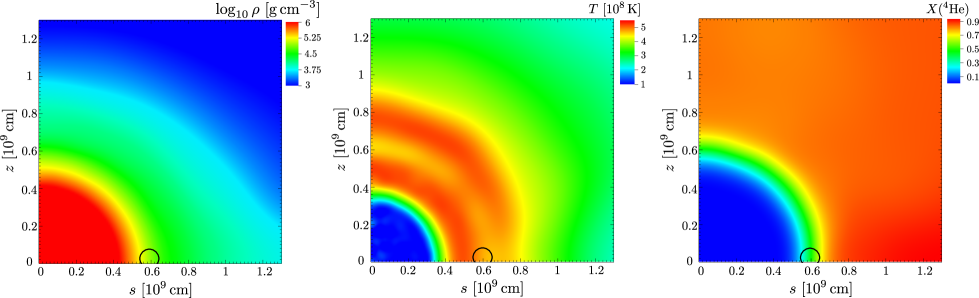
Figure 1: Density (left), temperature (center) and the helium mass fraction (right) after the mapping onto the 2D cylindrical grid for the merger remnant of an initial system with $0.45+1.1\,M_{\odot}$ components. For this particular system, the three search criteria ($C_{1}-C_{3}$) return a single hotspot, located in the first quadrant and represented with a circle of 500 km radius.

All calculations have been carried out in 2D cylindrical geometry, taking rotation into account (so-called “2.5D” approach). The computational domain is divided into blocks (16 in both $s$- and $z$-direction, where $s$ is the cylindrical radius and $z$ is the height), each containing $[16\times 16]$ computational zones. Five levels of refinement were allowed, yielding an effective grid size of $[4096\times 4096]$ or 2.7 km for a domain extending up to $1.1\times 10^{9}$ cm. Lower and larger grid sizes are also used, between $1.0-1.5\times 10^{9}\,{\rm cm}$, depending on the mass ratio between the donor and the accretor, $q=M_{2}/M_{1}$: lower/higher would produce a more/less extended remnant.

For the models where a detonation is ignited, we rerun the simulations with an extended computational domain of $s_{\rm max}=z_{\rm max}=10^{11}$ cm. This allows us to follow the nucleosynthesis processes until the ejecta reaches the homologous phase. For these runs, we have changed the grid parameters to nine levels of refinement and $[32\times 32]$ computational zones/block in order to yield an effective grid resolution of 7.6 km.

2.1 Initial models

For our initial models, we use the WD-WD parameter space studies of Dan et al. (2012, 2014). We follow the evolution of nine systems, representing all possible chemical composition combinations in the WD-WD parameter space. We choose the following WD compositions: pure He for $M_{\rm WD}\leq 0.45\,M_{\odot}$; a hybrid composition consisting of an CO ($X[\!\,^{12}{\rm C}]=0.5$, $X[\!\,^{16}{\rm O}]=0.5$) core surrounded by a pure He envelope of $0.1\,M_{\odot}$ for $0.45\,M_{\odot}<M_{\rm WD}\leq 0.6\,M_{\odot}$; pure CO ($X[\!\,^{12}{\rm C}]=0.4$, $X[\!\,^{16}{\rm O}]=0.6$) for $0.6\,M_{\odot}<M_{\rm WD}\leq 1.05\,M_{\odot}$ and made of ONe and magnesium (Mg) ($X[\!\,^{16}{\rm O}]=0.6,\ X[\!\,^{20}{\rm Ne}]=0.35$ and $X[\!\,^{24}{\rm Mg}]=0.05$) for $M_{\rm WD}\geq 1.05\,M_{\odot}$. As the maximum temperature inside the remnant tends to increase with the total mass (Zhu et al., 2013; Dan et al., 2014), from each of these nine regions, we choose one of the most massive WD-WD remnants:

• $\mathbf{0.45+0.45\,{M}_{\odot}}$ – largest total mass of two WDs that are made of He;

• $\mathbf{0.45+0.6\,M_{\odot}}$ – largest mass combination of a WD made of He and a hybrid one, made of He and CO;

• $\mathbf{0.45+0.9\,M_{\odot}}$ – largest He with a massive CO;

• $\mathbf{0.45+1.1\,M_{\odot}}$ – largest He with a massive WD made of ONe;

• $\mathbf{0.55+1\,M_{\odot}}$ – massive hybrid He-CO WD with massive CO WD;

• $\mathbf{0.6+0.6\,M_{\odot}}$ – most massive hybrid He+CO WD system;

• $\mathbf{0.6+1\,M_{\odot}}$ – massive hybrid He-CO WD with a massive WD made of ONe;

• $\mathbf{0.95+1.15\,M_{\odot}}$ – massive CO plus massive WD made of ONe;

• $\mathbf{1.05+1.05\,M_{\odot}}$ – largest total mass of two CO WDs.

The 3D WD-WD merger remnants from Dan et al. (2014) are mapped onto a 2D axisymmetric cylindrical Eulerian mesh, with the averaging done over the azimuthal angle $\phi$. The snapshots are taken at a time of three initial orbital periods after the moment when the donor is fully disrupted. At this stage the dynamical evolution is essentially over. The result of the mapping can be seen in Figure 1 for the $0.45+1.1\,M_{\odot}$ system.

We run three sets of simulations:

1. In a first set, we investigate whether the WD remnants could lead to detonations shortly after the restart of the simulations with FLASH, without any change of their properties (i.e., no perturbations). Runs are ordered by increasing donor’s mass and by decreasing mass ratio q and labeled 1 through 9. The main properties of this set of runs are listed in Table A1.

2. Through mapping, there is a loss of resolution because first, the SPH interpolation is required to get the values on the grid and second, an averaging is done over the azimuthal angle. This has an impact onto the thermal evolution of the remnant as the hotspots are smoothed out and chemical compositions change, especially inside chemically mixed regions. This motivates the second set of runs (initial conditions are presented in Table A2), where we manually setup hotspots based on different criteria guided by the 3D SPH simulations: ${C_{1}}$ uses the ratio between the nuclear and dynamical timescales $\tau_{\rm nuc}/\tau_{\rm dyn}(T)$ (effective timescales are computed as in Dan et al., 2012); ${C_{2}}$ uses the maximum temperature over all particles $T_{\rm max}$, and ${C_{3}}$ uses the maximum temperature over particles above a threshold density of $10^{5}\,{\rm g\,cm^{-3}}$, $T_{\rm max}(\rho\geq{10^{5}}\,{\rm g\,cm^{-3}})$, respectively. For CO mass-transferring systems besides criteria $C_{1}$ and $C_{2}$, we also use $T_{\rm max}(\rho\geq 10^{6}\,{\rm g\,cm^{-3}})$ (${C_{4}}$). For this set of runs, all SPH particles are searched to locate the one satisfying the condition specified by the selection criteria. Its position $(s_{\rm per},z_{\rm per})$ and temperature ($T_{\rm per}$) are used to setup the hotspot, see below for more details. Models are ordered in the same way as for the previous set, only that after the run number the search criteria ($C_{1}-C_{4}$) was added. For example, run 4 ($0.45+1.1\,M_{\odot}$) using the results of the hotspot search criteria $C_{1}$ was named “4.c1”.

3. Finally, for the third set of tests (see Table A3), the hotspots are setup following the critical conditions for a spontaneous initiation of a detonation from the spatially resolved 1D calculations of Holcomb et al. (2013) and Shen & Moore (2014) for He composition and Röpke et al. (2007) and Seitenzahl et al. (2009) for CO. For this set of runs, we assume that the systems have evolved to reach the conditions necessary for spontaneous detonations determined in the previously cited studies, as the spatial scales relevant for the initiation of the He or CO detonations cannot be resolved in our multidimensional simulations (He and C detonation length scales, at densities above $\rho=10^{7}\,{\rm g\,cm^{-3}}$, are below $10^{4}$ cm and 1 cm, respectively; Holcomb et al., 2013; Shen & Bildsten, 2014). For He mass transferring tests we setup hotspots with the following properties: a temperature perturbation of $5\times 10^{8}$ K (or $8\times 10^{8}$ K, if the hot envelope temperature is close to $5\times 10^{8}$ K) at densities above $3-5\times 10^{5}\,{\rm g\,cm^{-3}}$. This is what sets a direct detonation below a perturbation radius of about $R_{\rm per}=1000$ km (Holcomb et al., 2013; Shen & Moore, 2014). For the CO mass-transferring systems, we use $T_{\rm per}=3\times 10^{9}$ K at densities above $\rho=1\times 10^{6}\,{\rm g\,cm^{-3}}$. Models are ordered in the same way as above, with the label “dd” (an abbreviation to indicate “direct detonation”) added after the run number.

Seitenzahl et al. (2009) explored the effect of different initial profiles for density, temperature and chemical composition on the spontaneous initiation of CO detonations and found that the different profiles change the hotspots critical sizes. For the runs with perturbations, we also test the impact of the hotspot temperature and composition profiles (see §2.3 and 2.2), and, because our calculations are in 2D cylindrical geometry, the impact of hotspot geometry (see §2.5). While we carefully choose where to place the hotspots and test the different setups, further explorations are required as several assumptions are made here. For example, it is not clear how the ignition of a detonation may depend on the time dependence of the hotspot formation. Our setups for the second and third set of tests is based on the main assumption that hotspots with properties (presented in Section 3) close to those leading to the core detonation develop during the WD merger remnants evolution. The second set of tests is based on a realistic approach, but we still have modified the hotspots temperature profiles, both, in extent and shape. For the third set, the assumptions were further relaxed, with hotter hotspots placed in denser regions of the envelope. Probably, such conditions could be realised only if the initial spin state of the WDs would be different. For example, it has been shown in Zhu et al. (2013); Dan et al. (2014) that starting with non-rotating initial stars the location of peak temperature is located in a denser environment compared to when starting with corotating stars, like in the present study. The effect of the initial conditions will be investigated in a future study.

2.2 Hotspot size

For the runs with perturbations (second and third sets) our strategy is to start with a relatively large perturbation radius inside the shell of $R_{\rm per}=1000$ km. Such initial large hotspots are unrealistic and are not seen in the SPH simulations of WD mergers and they are more characteristic to WD collisions (Rosswog et al., 2009a; Raskin et al., 2009; Aznar-Siguán et al., 2013; Kushnir et al., 2013; García-Senz et al., 2013; Papish & Perets, 2015). The SPH interaction radius of the particles inside the hot envelope is below $\sim\!1000$ km, decreasing with increasing density, towards the core where the hotspots are located. If a detonation is triggered into the underlying core, we repeat the simulations with a new hotspot radius $R_{\rm per}$ which is determined by the bisection root-finding method. We repeat this process until the core does not detonate anymore and the difference between the hotspot radius of a successful and failed run is below $15\%$. The minimum perturbation radius $R_{\rm per}$ at which the core detonates is included in Tables 3.1 and 3.2. We note that the minimum value thus obtained is method- and ICs-dependent and can change with the star’s spin and chemical composition, numerical resolution and the nuclear reaction network (see a detailed discussion of these factors in Section 3).

2.3 Hotspot temperature profile

The initial temperature profile from the SPH simulations can take different shapes. If not specified otherwise, the hotspots are setup with a flat temperature profile, i.e., constant temperature $T_{\rm per}$ inside the perturbation radius $R_{\rm per}$. To test the dependence on the temperature profile, in addition to the flat temperature profile, we setup hotspots using a linear profile

$$T(r)=\left\{\begin{array}[]{ll}T_{\rm per}-\frac{T_{\rm per}-T_{\rm amb}}{R_{\rm per}}r&\textrm{for $r\leq R_{\rm per}$,}\\ \\ T_{\rm per}&\textrm{for $r>R_{\rm per}$,}\end{array}\right.$$ (1)

as well as Gaussian

$$T(r)=T_{\rm amb}+(T_{\rm per}-T_{\rm amb})e^{-(r/R_{\rm per})^{2}},$$ (2)

where $r$ is the distance from the hotspot origin and $T_{\rm amb}$ is the ambient temperature, chosen as the highest temperature in the neighbour cells, surrounding the hotspot.

2.4 Hotspot composition

The mixing of matter between the binary components causes the composition to be inhomogeneous mainly through the outer layers of the core, the hot envelope and the inner disk. It occurs mainly during the last phase of the merging process and it tends to increase with the mass ratio $q=M_{\rm don}/M_{\rm acc}$ (Zhu et al., 2013; Dan et al., 2014). Only two regions of the parameter study have both stars made of the same fuel: He–He and CO–CO. The other regions are made of a combination of He, CO and ONe.

The third panel of Figure 1 shows the mass fraction of He for a $0.45+1.1\,M_{\odot}$ system. For this system, the hotspot search criteria $C_{1}$ returns a particle with mainly CO neighbour particles (i.e., particles contributing to the interpolation), but also $\sim\!15\%$ made of pure He. Similar to the hotspot temperature, discussed in the previous section, after the mapping onto the 2D grid some details about the mixing are lost and, in some cases, the fuel (He or CO) concentration is reduced to very low numbers. Specifically, for the models with $0.55+1\,M_{\odot}$ and $0.6+1.1\,M_{\odot}$ initial components, there is a lack of He fuel ($X[\,\!^{4}{\rm He}]<0.1$) inside the hot envelope at densities above $\rho\geq 6\times 10^{4}\,{\rm g\,cm^{-3}}$ and $\rho\geq 3.9\times 10^{4}\,{\rm g\,cm^{-3}}$, respectively. For these two systems we have set the hotspot composition to pure He.

2.5 Hotspot geometry

In 2D cylindrical geometry, the hotspots are tori extending around the star. For the $0.45+0.6\,M_{\odot}$ and $0.45+0.9\,M_{\odot}$ systems we have also setup spherical hotspots, i.e., the perturbation was placed at the pole, i.e., where $s=0$ (run 2.dd-Polar and 3.dd-Polar, respectively, see Table 3.2). Also for these two tests, we determine the minimum perturbation radius leading to a (core) detonation through bisection.

3 Results

3.1 Models without perturbation

Run	Initial	$T_{\rm max,8}$	$\rho_{5}(T_{\rm max})$	Ignition		$t_{\rm det.env,s}$	$t_{\rm det.core,s}$	Comments
missingmissingmissing  5-6
No	masses [$M_{\odot}$]	Envelope	Core
Helium mass transferring systems
1	$0.45+0.45$	2.786	0.009	No	No	-	-	$\rho$(hot envelope) too low, no burning
2	$0.45+0.6$	2.822	0.051	No	No	-	-	$\rho$(hot envelope) too low, no burning
3	$0.45+0.9$	5.781	0.358	No	No	-	-	$\rho$(hot envelope) too low, no burning
4	$0.45+1.1$	19.581	2.007	Yes	No	1.3	-	core intact, envelope burns mainly
								to IMEs and some IGEs
5	$0.55+1.0$	6.556	1.041	No	No	-	-	no burning, very little He left inside
								hot envelope after mapping
6	$0.6+0.6$	4.035	1.120	No	No	-	-	little burning inside hot envelope
7	$0.6+1.1$	8.158	1.165	No	No	-	-	temperature inside hot envelope high,
								but little He there ($X(\,\!^{4}{\rm He})_{\rm max}\!\approx\!10^{-3}$);
								some burning (small amount of IMEs)
Carbon/oxygen mass transferring systems
8	$0.95+1.15$	11.561	9.493	No	No	-	-	temperature too low; little burning
9	$1.05+1.05$	11.172	0.731	No	No	-	-	temperature too low; little burning

Table 1: Outcomes for the first set of runs, without perturbation: masses ($M_{\odot}$) at the beginning of mass transfer, when the simulations are initialised in SPH; maximum temperature $T_{\rm max,8}$ (in units of $10^{8}$ K) and density at the location of maximum temperature $\rho_{5}(T_{\rm max,9})$ (in units of $10^{5}\,{\rm g\,cm^{-3}}$) during the entire evolution; $t_{\rm det.env,s}$ and $t_{\rm det.core,s}$ are the time (in units of s) after which a detonation is ignited in the envelope and in the core, respectively.

A summary of the outcome for this set of runs is presented in Table 3.1. Only the $0.45+1.1\,M_{\odot}$ system triggers a (He) shell detonation. Shocks propagate through the underlying (ONe) core, but the temperature is not hot enough to fuse oxygen. The nucleosynthetic yields for this run are shown in the fourth column of Table A4, in the Appendix. The yields are low and the majority of burning products are in the form of intermediate-mass elements (IMEs; with the atomic mass number $A$ ranging from 28 to 40), with very low yields of iron-group elements (IGEs; with $A\geq 44$). Most of the He remains unburned (initial He mass of $M(\,\!^{4}{\rm He})=0.45\,M_{\odot}$). This will be a very faint event, much fainter than a “point” Ia supernova (Shen et al., 2010). The main reasons why the other systems containing He do not trigger a detonation without a perturbation is that the hot regions (i.e., envelope) in some of our merger remnants have typical densities of $\rho\sim 10^{5}\,{\rm g\,cm^{-3}}$ and detonations are not expected to be ignited at this density. Woosley & Kasen (2011), assuming that the accreted material is made of 99% $\,\!{}^{4}{\rm He}$ and 1% $\,\!{}^{14}{\rm N}$, have shown that He does not directly ignite a detonation below a density of $\sim 10^{6}\,{\rm g\,cm^{-3}}$, unless the hotspot size is a significant fraction of the WD scale height. Holcomb et al. (2013) reached a similar conclusion assuming a pure He composition of the burning region. However, the envelopes in our models, containing initially a (hybrid) He mass-tranferring star and a (hybrid) CO accretor, are not made of pure He, but a mixture of He and CO. It has been shown that by adding a fraction of CO to the He hotspot, depending on the temperature, the hotspot size could be reduced by more than an order of magnitude (Shen & Moore, 2014). The hotspot size could be further reduced if instead of using the “aprox13” network, we would use a large reaction network in order to allow for the $(p,\gamma)(\alpha,p)$, with the proton playing a catalytic role near the beginning of the $\alpha$-chain (Woosley & Kasen, 2011; Shen & Moore, 2014). We defer a study of the effects of a larger network to future research.

For the CO systems, we have found that after the mapping onto the 2D grid, the systems have temperatures below the threshold for carbon-ignition. For those with a hybrid He+CO former donor ($0.55+1\,M_{\odot}$ and $0.6+1.1\,M_{\odot}$) there is a lack of He fuel inside the hot envelope. While temperatures and densities are high inside the hot envelope (see Table A1), the He mass fraction is very low $X(\,\!^{4}{\rm He})<0.1$.

Run	Initial	$R_{\rm per,km}$	$T_{\rm max,8}$	$\rho_{5}(T_{\rm max})$	Ignition		$t_{\rm det,s}$	$t_{\rm det.core,s}$	Comments
missingmissingmissing  6-7
No	masses [$M_{\odot}$]	Envelope	Core
Helium mass transferring systems
1.c1	$0.45+0.45$	1000	2.786	0.009	No	No	-	-	$\rho$(hot envelope) too low
missingmissingmissing  1-1
missingmissingmissing  3-9
1.c2	1000	2.920	0.009	No	No	-	-	no burning
missingmissingmissing  1-1
missingmissingmissing  3-9
1.c3	1000	2.781	0.009	-	-	-	-
2.c1	$0.45+0.6$	1000	2.760	0.061	No	No	-	-	little He burning in
missingmissingmissing  1-1
missingmissingmissing  3-9
2.c2	1000	3.353	0.130	No	No	-	-	and around hotspot
missingmissingmissing  1-1
missingmissingmissing  3-9
2.c3	1000	2.838	0.042	No	No	-	-
3.c1	$0.45+0.9$	1000	6.857	0.462	No	No	-	-	envelope perturbed;
3.c3									He burning in and around
missingmissingmissing  1-1
missingmissingmissing  3-9
3.c2	1000	6.294	0.448	No	No	-	-	hotspot region
4.c1	$0.45+1.1$	500	67.758	801.038	Yes	Yes	0.34	1.74	core ignited off-center and burns
4.c2									up to $\,\!{}^{56}{\rm Ni}$; envelope burns
									mainly to IMEs, little to IGEs
missingmissingmissing  1-1
missingmissingmissing  3-10
4.c3	-	-	-	-	-	-	-	no run as $T_{\rm per}\approx T_{\rm grid}$
5.c1	$0.55+1.0$	1000	10.393	1.491	No	No	-	-	little burning (no IGEs) around
5.c2									hotspot region; initial
5.c3									$X(\,\!^{4}{\rm He})_{\rm max}\!\approx\!10^{-3}$ inside hotspot
6.c1	$0.6+0.6$	1000	3.951	0.880	No	No	-	-	envelope perturbed by initial
6.c2									wave-like shocks, but only
6.c3									little burning going on
7.c1	$0.6+1.1$	1000	8.085	1.962	No	No	-	-	similar evolution with run 7
7.c3
missingmissingmissing  1-1
missingmissingmissing  3-10
7.c2	1000	8.125	1.179	No	No	-	-	evolution similar with run 7
								but envelope more perturbed
Carbon/oxygen mass transferring systems
8.c1	$0.95+1.15$	1000	12.798	6.607	No	No	-	-	envelope perturbed; little burning
inside envelope
missingmissingmissing  1-1
missingmissingmissing  3-10
8.c2	1000	13.004	10.876	No	No	-	-	similar evolution with run 8.c1
8.c4
9.c1	$1.05+1.05$	1000	10.414	64.259	No	No	-	-	similar with run 9;
9.c2									burning only inside hotspot’s
9.c4									higher density region

Table 2: Outcomes for the second set of runs, with perturbation based on different criteria guided by the 3D SPH simulations: same quantities as in Table 3.1, only the hotspot radius $R_{\rm per,km}$ (in units of km) has been added.

3.2 Models with perturbation based on SPH calculations guided criteria

A summary of the outcome for this set of runs is presented in Table 3.1. With perturbations set based on the hotspot search criteria guided by the 3D SPH simulations presented in Section 2.1, again, only the $0.45+1.1\,M_{\odot}$ system detonates (run 4.c1). For this system, the criteria $C_{1}$ and $C_{2}$ return the same hotspot, close to the orbital plane ($s=0.595\times 10^{9}$ cm and $z=0.026\times 10^{9}$ cm). The difference, compared to the model without perturbation, run $4$, is that in this case also the (ONe) core detonates, see the upper panels of Figure 2. As discussed in Section 2.2, we start with a relatively high perturbation radius and then decrease it through successive bisections, until the difference between hotspot radius of a succesful and a failed run is below $15\%$. For this case, the minimum perturbation radius at which the second detonation is triggered is $R_{\rm per}=500$ km. Above this value, the evolution is the same: triple alpha reactions quickly raise the temperature to $\sim 1.9\times 10^{9}$ K so that a large overpressure is produced. A self-sustained detonation is formed, which wraps around the (ONe) core and converges inside the core close to the polar axis (due to the cylindrical symmetry of our models). At that point, the shock wave is sufficiently strong to cause a shock-initiated off-center core detonation. The ONe detonation occurs when a spherical region ($z=1950$ km and $r\approx 0$) of a $(100\ {\rm km})$ radius reaches a temperature of $T\approx 6\times 10^{9}$ K at a density of $\rho\approx 4\times 10^{7}\,{\rm g\,cm^{-3}}$. The robustness of the ONe core detonation is further discussed in Section 3.5.

For all He mass-transferring systems, we have run two extra sets of simulations with an increased density threshold of $\rho\geq 5\times 10^{5}\,{\rm g\,cm^{-3}}$ and $\rho\geq 1\times 10^{6}\,{\rm g\,cm^{-3}}$, but without success. Above these thresholds the temperatures are either too low or there is no or very little He inside the hotspots. We also run tests using multiple hotspots for the systems returning different hotspots criteria: $0.45+0.9\,M_{\odot}$ with two hotspots set according to the results of the search criteria $C_{1}$ ($C_{2}$ returns the same hotspot) and $C_{3}$ and $0.95+1.15\,M_{\odot}$ with two hotspots based on $C_{1}$ and $C_{2}$ ($C_{4}$ returns the same hotspot). Also for these runs a detonation was not ignited.

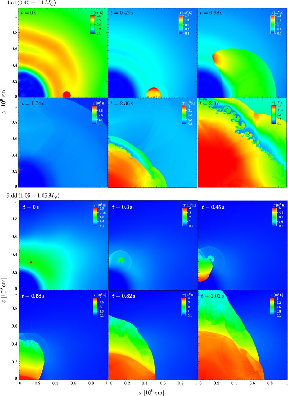
Figure 2: Evolution of the $0.45+1.1\,M_{\odot}$ (run number 4.c1; upper panels) and $1.05+1.05\,M_{\odot}$ (run number 9.dd; lower panels) systems. Color coded is the temperature in units of $10^{9}\,{\rm K}$.

Run	Initial	$R_{\rm per,km}$	$T_{\rm max,9}$	$\rho_{6}(T_{\rm max})$	Ignition		$t_{\rm det.env,s}$	$t_{\rm det.core,s}$
missingmissingmissing  6-7
No	masses [$M_{\odot}$]	Envelope	Core
Helium mass transferring systems
1.dd	$0.45+0.45$	437.5	4.297	4.656	No	Yes	-	2.2
2.dd	$0.45+0.6$	875	8.262	56.471	Yes	Yes	0.3	0.3
2.dd-Polar	$0.45+0.6$	156.25	8.211	53.964	Yes	Yes	0.11	0.2
3.dd	$0.45+0.9$	187.5	5.682	21.966	Yes	Yes	0.1	1.8
3.dd-Polar	$0.45+0.9$	750	5.856	30.337	Yes	Yes	0.17	2.7
5.dd	$0.55+1$	500	6.435	36.552	Yes	Yes	0.1	0.24
6.dd	$0.6+0.6$	375	3.188	4.740	No	Yes	-	1
7.dd	$0.6+1.1$	1000	5.178	21.104	Yes	No	0.1	-
Carbon/oxygen mass transferring systems
8.dd	$0.95+1.15$	500	9.447	112.052	No	Yes	-	0.33
9.dd	$1.05+1.05$	125	6.228	40.736	No	Yes	-	0.3

Table 3: Outcomes for the third set of runs, where the hotspots are setup following the critical conditions for a direct initiation of a detonation from the spatially resolved 1D calculations. Same quantities as in Table 3.1, only that the temperare is in units of $10^{9}$ K and density in units of $10^{6}\,{\rm g\,cm^{-3}}$.

The fifth column of Table A4 in the Appendix shows the nucleosynthetic yields for this run and the upper panels of Figure 3 show the final abundance distribution in velocity space. This model should resemble a “normal” SN Ia. The isotope yields are very similar to those of Moll & Woosley (2013) for the system with $0.81+0.96\,M_{\odot}$ (see their Table 3) and with those of Pakmor et al. (2012) for their $0.9+1.1\,M_{\odot}$ (see Section 3 in Pakmor et al., 2012). However, our model leads to a different ejecta morphology compared with that of Pakmor et al. (2012) and Moll & Woosley (2013). While they find IMEs and unburned oxygen at the center of the ejecta and $\,\!{}^{56}{\rm Ni}$ above this region (see their Figure 9), our model leads to a SN Ia-like ejecta structure (Mazzali et al., 2007). Similar to Moll & Woosley (2013), the ejecta in our model is asymmetric with a higher velocity along the polar regions compared to the equatorial ones. This should lead to orientation effects for both light-curves and spectra, see the detailed discussion of synthetic observables in Section 4 of Moll & Woosley (2013). The reasons that the other systems fail to detonate are the same as presented above, for the runs without perturbation: the hotspots temperature and/or density are either too low or there is no or very little He inside the hotspots.

3.3 Models with perturbation based on 1D spatially resolved calculations

Detonations are triggered for all runs starting with hotspots following the critical conditions for a spontaneous initiation of a detonation from the spatially resolved 1D calculations of Holcomb et al. (2013); Shen & Moore (2014) for He composition and Röpke et al. (2007); Seitenzahl et al. (2009) for CO.

Before we discuss the models in detail, we outline some of the general findings, characteristic to the majority of the models. In general, the second detonation happens either through a smooth transition from the envelope into the core (edge-lit detonation scenario) or a second detonation occurs after shock convergence into the core (off-center detonation scenario). However, not all systems undergo double detonations. For run 1.dd ($0.45+0.45\,M_{\odot}$), the hotspot is set inside the core. This setup system is very improbable, at least for the initial conditions (tidally locked stars) used in the calculations of Dan et al. (2012, 2014). Because the hot envelope has a low density ($\rho_{\rm env}<10^{5}\,{\rm g\,cm^{-3}}$), in order to trigger a detonation we have to setup a hotspot inside the cold core, in the equatorial plane, $\approx 5400$ km above the core’s center (1500 km below the location of $T_{\rm max}$). The evolution is very similar for runs 6.dd ($0.6+0.6\,M_{\odot}$) and 9.dd ($1.05+1.05\,M_{\odot}$). The perturbation does not lead to a shell detonation, but to a sub-sonic shock wave which reflects at the pole, at the core’s edge and triggers a direct detonation there.

The lower panels of Figure 3 show the final nuclear mass fractions of $\!\,{}^{12}{\rm C}$, $\!\,{}^{16}{\rm O}$, $\!\,{}^{28}{\rm Si}$ and $\!\,{}^{56}{\rm Ni}$ in the velocity space for the $1.05+1.05\,M_{\odot}$ system. While the outer ejecta (i.e., unburned matter) are more or less symmetrically propagating into the ambient medium, the IGEs have higher ejecta velocities in the polar direction. The most extended shock front (i.e., contact surface between the ejecta and the low-density ambient matter) is obtained for the most energetic explosions (Figure 6). The interaction of the ejecta with the low density ambient gives rise to Rayleigh-Taylor hydrodynamic instabilities behind the shock front, when the denser layers penetrate the overlying lighter ambient environment.

Run	Temp.	$T_{\rm max,8}$	$\rho_{5}(T_{\rm max})$	Ignition		$t_{\rm det.env,s}$	$t_{\rm det.core,s}$
missingmissingmissing  5-6
	profile	Envelope	Core
4.c1-TH	Top hat	58.889	519.168	Yes	Yes	0.1	1.54
4.c1-Linear	Linear	19.308	1.950	Yes	No	1.3	-
4.c1-Gaussian	Gaussian	59.914	655.004	Yes	Yes	0.28	1.7

Table 4: Dependence on the temperature profiles. The comparison is done for the succesful detonating $0.45+1.1\,M_{\odot}$ system, using a perturbation radius $R_{\rm per}$ of 1000 km and the conditions returned by the criteria $C_{1}$. The ambient temperature corresponds to the maximum temperature on the grid cells surrounding the hotspot.

Run 2.dd ($0.45+0.6\,M_{\odot}$), 3.dd ($0.45+0.9\,M_{\odot}$) and run 7.dd ($0.6+1.1\,M_{\odot}$) produce little $\,\!{}^{56}{\rm Ni}$, between 0.01 and $0.09\,M_{\odot}$, and they would be faint and lie outside the range of “normal” SNe Ia. Run 7.dd is the only model where a second detonation in the (ONe) core could not be triggered (maximum $R_{\rm per}=1000$ km).

For the $0.6+0.6\,M_{\odot}$ system, the initial shock wave triggers a direct detonation at the core’s edge (outer regions of the core are made from a mixture of CO and He). Very little $\,\!{}^{56}{\rm Ni}$ is produced and will thus produce a very faint supernova, powered mainly by the decay of $\,\!{}^{48}{\rm Cr}$. The composition of the ejecta is similar to the model 8HBC1 of Woosley & Kasen (2011), although their model is a result from a He detonation. Their model give rise to a dim fast evolving event (peak magnitude in B-band of -13.5) resembling the spectra of sub-luminous SNe, such as SN 1991bg.

Our best candidates to reproduce a “normal” SN Ia are the ${0.45+1.1\,M_{\odot}}$ (run 4.c1, discussed above) and the ${1.05+1.05\,M_{\odot}}$ (run 9.dd) systems. For the $1.05+1.05\,M_{\odot}$ system, the isotope yields and the kinetic energy of the ejecta are very similar to those of Moll & Woosley (2013) for the system with $0.81+0.96\,M_{\odot}$. The difference in the IMEs mass is of less than 1% and in the IGEs of less than 10%, with their calculations leading to a larger amount of $\,\!{}^{56}{\rm Ni}$, ($\sim\!7\%$ by mass). Our model leaves more unburned material ($50\%$ more C and $30\%$ more O), as the total mass is larger in our case ($2.1$ vs $1.77\,M_{\odot}$ in Moll & Woosley, 2013). However, the ejecta morphology is very different from Moll & Woosley (2013), where the detonation is triggered at the merger moment, when the secondary star has not been disrupted yet. The main difference is that in the model of Moll & Woosley (2013) the material located at the center of the supernova remnant is coming from the former secondary, relatively low density WD. While there is a high abundance of IMEs, no $\,\!{}^{56}{\rm Ni}$ is being produced. In our model the ejecta has a SN Ia-like structure (Mazzali et al., 2007), with IGEs (mainly $\,\!{}^{56}{\rm Ni}$) at the center surrounded by IMEs and unburned material in the outer parts of the ejecta. This nucleosynthesis of this model also compares well with the $0.9+1.1\,M_{\odot}$ system from Pakmor et al. (2012), just that, again, the ejecta morphology is different. Their model is more similar to Moll & Woosley (2013), with the material of the former secondary WD dominating the central ejecta, and thus no IGEs in the core. The more massive ${0.95+1.15\,M_{\odot}}$ system produces an abundance of $\,\!{}^{56}{\rm Ni}$ ($0.82\,M_{\odot}$) and will most likely produce a bright SN Ia. As discussed in Moll & Woosley (2013), due to the asymmetry of the ejecta, the brightness of this model will further be boosted in the direction where $\,\!{}^{56}{\rm Ni}$ is closer to the observer and that could account for the apparent excess mass in the “super-Chandrasekhar” events. A detailed comparison of the nucleosynthetic yields from our models and those inferred from the observations is presented in Section 3.5.

3.4 Hotspot geometry and composition

For two systems, with $0.45+0.6\,M_{\odot}$ and $0.45+0.9\,M_{\odot}$ components, we have placed the hotspot at the pole. With this setup, the hotspot has a spherical shape compared to the torus geometry (by virtue of the cylindrical symmetry) of the other models.

For the $0.45+0.6\,M_{\odot}$, run 2.dd-Polar in Table 3.2, He detonates soon after the start of the simulation ($t=0.13$ s) and there is a smooth transition to an edge-lit CO core detonation at $t\approx 0.19$ s. The reduced perturbation radius translates into a reduced perturbation energy required to trigger a second detonation in the core by almost four orders of magnitude. This could be explained by the more favorable composition compared to run 2.dd. At the location of the hotspot, the envelope is not made of pure He, but a mixture between He ($X[\!\,^{4}{\rm He}]\sim 0.6$), C ($X[\!\,^{12}{\rm C}]\sim 0.2$) and O ($X[\!\,^{16}{\rm O}]\sim 0.2$), while the outer region of the core where the CO detonation is triggered, the composition is dominated by C ($X[\!\,^{12}{\rm C}]\sim 0.4$) and O ($X[\!\,^{16}{\rm O}]\sim 0.4$), but mixed with He ($X[\!\,^{4}{\rm He}]\sim 0.4$) (see Seitenzahl et al. (2009); Shen & Moore (2014) for a discussion on the effects of composition on the detonation).

For the $0.45+0.9\,M_{\odot}$ system, run 3.dd-Polar in Table 3.2, while the perturbation radius has to be larger to triggere a second detonation in the core compared to run 3.dd, the deposited energy is almost the same ($5.7$ and $1.6\times 10^{46}$ for 3.dd and 3.dd-Polar, respectively). A He-detonation is triggered after 0.17 s in the upper part of the hotspot, where there is more He ($X[\!\,^{4}{\rm He}]\sim 0.7$). It propagates around the core and it reflects at the $z=0$ symmetry axis after 1.23 s. Shock waves from the He detonation trigger a second detonation but only after 2.7 s, at the symmetry axis $s=0$ and $z\approx 1200$ km above the core’s center.

The dependence on the temperature profiles of the hotspot has also been tested. The results of the different setups using a flat, linear and Gaussian profiles are shown in Table 3.3. The different profiles models follow the same setup as run 4.c1 (see Table A2 in the Appendix), only that here we do not determine the minimum size $R_{\rm per}$ of the hotspot, but run a single test for each profile using $R_{\rm per}=1000$ km. The “top-hat” profile (run 4.c1-TH) more readily leads to a detonation, shortly ($<0.1$ s) after the simulation are started, the Gaussian profile (run 4.c1-Gaussian) takes longer to initiate the envelope detonation and subsequently the core detonation, while for the linear profile (run 4.c1-Linear), a detonation is triggered only in the envelope and only after a delay of 1.3 s. The difference in the evolution of the three models is caused by the density profiles inside the hotspots. As the density increases from the center of the hotspot in the direction towards the core, only the “top-hat” and Gaussian profiles have a high enough temperature at a high enough density so that the detonation can quickly emerge.

3.5 Nucleosynthetic yields

Table A4 lists the nucleosynthetic yields of all successfully detonating models. Also shown in Table A4, are the final kinetic energies and the sum of the masses of IMEs and IGEs. Using these and the ejecta composition structure in velocity space, we constrain our models with a set of observations presented below. We are using the upper limits placed on the $\!\,{}^{44}{\rm Ti}$ mass from the observations of Tycho’s (Lopez et al., 2015) and G1.9+1.3’s (Zoglauer et al., 2015) remnants, the ejecta velocity of the Si II $\lambda 6355$ and Ca II H&K features and the total amount of $\!\,{}^{28}{\rm Si}$, $\!\,{}^{40}{\rm Ca}$ and $\!\,{}^{56}{\rm Ni}$ synthesised.

To date, there is no direct detection of $\!\,{}^{44}{\rm Ti}$ in the SN Ia remnants, but there have been upper limits set on the presence of $\!\,{}^{44}{\rm Ti}$. Lopez et al. (2015), using NuSTAR observations of Tycho’s remnant, have found an upper limit between 0.47 and $4.1\times 10^{-4}\,M_{\odot}$, increasing with the distance to the remnant. We have also estimated an upper limit for $\!\,{}^{44}{\rm Ti}$ in G1.9+1.3, the most recent supernova (most likely a Type Ia Borkowski et al., 2010; Yamaguchi et al., 2014) in the Milky Way. We used the distance inferred by Reynolds et al. (2008) based on an analysis of the absorption toward G1.9+0.3, but lower and higher values are possible (e.g., Roy & Pal, 2014). We use the formula presented in Lopez et al. (2015) to convert flux in the 68 keV to a $\!\,{}^{44}{\rm Ti}$ mass, where the flux was determined from Figure 6 of Zoglauer et al. (2015) using a line-width of $1.4\times 10^{4}\,{\rm km\,s^{-1}}$ (or 3 keV at 68 keV) (Reynolds et al., 2008) and a distance of 8.5 kpc.

In the right panel of Figure 4, we plot the $\!\,{}^{56}{\rm Ni}$ mass vs $\!\,{}^{44}{\rm Ti}$ mass for all detonating models together with the upper limits from the observations for the $\!\,{}^{44}{\rm Ti}$ mass. Only five models, located in Figure 4 at the left side with respect to the vertical lines, meet the constraint on $M(\!\,^{44}{\rm Ti})$: the two CO mass-transferring systems and the models involving an initial $0.45$ donor and a $0.9$ and $1.1\,M_{\odot}$ accretor.

A key constraint on the physical conditions in the SN Ia explosion is the $\!\,{}^{56}{\rm Ni}$ mass. The SNe Ia have a large range of luminosities as determined mostly by the amount of $\!\,{}^{56}{\rm Ni}$ that is synthesised in the explosion. The $\!\,{}^{56}{\rm Ni}$ mass can be determined directly from the observations assuming that it largely determines the peak bolometric luminosity (Arnett, 1982) and has a key role in understanding the peak luminosity decline-rate relation (Phillips, 1993). By modelling the late-time nebular spectra of SNe Ia, Stritzinger et al. (2006) have accurately measured the $\!\,{}^{56}{\rm Ni}$ mass for a set of 17 SNe Ia, ranging from the sub-luminous SN1991bg and up to the bright SN1991T, and found values between $0.08$ and $0.94\,M_{\odot}$. Piro et al. (2014), using the volume-limited sample of 74 SNe Ia from the Lick Observatory Supernova Search (LOSS; Li et al., 2011), found a very similar $\!\,{}^{56}{\rm Ni}$ range. The two closest SN Ia in decades, SN 2011fe (Nugent et al., 2011) and SN2014J (Fossey et al., 2014), are also within this range with values varying, depending on the method used to estimate them. For the SN2011fe, a $M({\!\,{}^{56}{\rm Ni}})=0.47\,M_{\odot}$ was derived from the nebular spectra (Mazzali et al., 2015) and a $M({\!\,{}^{56}{\rm Ni}})=0.53\pm 0.11\,M_{\odot}$ from the bolometric luminosity (Pereira et al., 2013). For SN 2014J, $M({\!\,{}^{56}{\rm Ni}})=0.62\pm 0.13\,M_{\odot}$ from the gamma-ray lines associated with $\!\,{}^{56}{\rm Co}$ decay and from the bolometric light curve $M({\!\,{}^{56}{\rm Ni}})$ within a range of $0.57\pm 0.2\,M_{\odot}$ as a function of the local extinction due to the ambient matter (Churazov et al., 2014).

Five models produce $M(\!\,^{56}{\rm Ni})$ between the observational limits for SNe Ia, as shown in the right panel of Figure 4). While run 3.dd ($0.45+0.9\,M_{\odot}$) will probably produce a sub-luminous SN Ia the other four runs produce a ${\!\,{}^{56}{\rm Ni}}$ mass typical for a “normal” SN Ia.

Another constraint on the detonating models comes from the mass of the IMEs of $\!\,{}^{28}{\rm Si}$ and $\!\,{}^{40}{\rm Ca}$. In a series of papers, using the code developed by Mazzali and collaborators, the abundance stratification of five SN remnants are approximated from a series of late (nebular) spectra assuming an initial density profile (from W7 and/or a delayed detonation model). Values for the $\!\,{}^{28}{\rm Si}$ and $\!\,{}^{40}{\rm Ca}$ masses are generally not given in these works, but they can be extracted from the “mass fractions vs. enclosed mass” figures provided, see Table 5. The values obtained for SN 2002bo, initially by Stehle et al. (2005), have been updated by Blondin et al. (2015) with a more accurate model, using non-local thermodynamic equilibrium time-dependent radiative-transfer simulations of a Chandrasekhar-mass delayed-detonation model and we use their values to constrain the models.

The $M(\!\,^{28}{\rm Si})$ range from $0.14\,M_{\odot}$ for SN 1991T (a peculiar, luminous SN Ia; Sasdelli et al., 2014) up to $0.31\,M_{\odot}$ for SN 2011fe (a “normal“ SN Ia; Mazzali et al. (2015)) and $M(\!\,^{40}{\rm Ca})$ from $8.3\times 10^{-4}\,M_{\odot}$ for SN 2011fe up to $0.045\,M_{\odot}$ for SN 2002bo (a “normal“ SN Ia; Blondin et al., 2015) In between these ranges are the SN 2003du, a normal SN Ia (Tanaka et al., 2011) and SN 2004eo, a SN Ia with a luminosity between normal and sub-luminous SNe Ia (Mazzali et al., 2008). In total, four models do no fit the $M(\!\,^{28}{\rm Si})$ and $M(\!\,^{40}{\rm Ca})$ range from the observations: single detonating models, run 4 and 7dd, the double He WD system 1.dd which is producing too little Si and 2.dd with slightly too much Ca (see Table A4).

SN	$M(\!\,^{28}{\rm Si})$	$M(\!\,^{40}{\rm Ca})$	Reference
	$[M_{\odot}]$	$[M_{\odot}]$
SN 2002bo	0.22	0.021	Stehle et al. (2005)
	0.31	0.045	Blondin et al. (2015)
SN 2004eo	0.41	$5.7\times 10^{-3}$	Mazzali et al. (2008)
SN 2003du	0.21	$1.4\times 10^{-3}$	Tanaka et al. (2011)
SN 1991T	0.14	0.017	Sasdelli et al. (2014))
SN 2011fe	0.31	$8.3\times 10^{-4}$	Mazzali et al. (2015)

Table 5: $\!\,{}^{28}{\rm Si}$ and $\!\,{}^{40}{\rm Ca}$ masses for five SNe Ia.

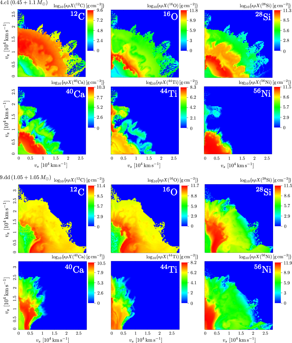
Figure 3: Final at ($t=39\,{\rm s}$) nuclear mass fractions ($s\rho X_{i}$, where $s$ is the cylindrical radius [in cm], $\rho$ is the density [in ${\rm g\,cm^{-3}}$] and $X_{i}$ is the mass fraction of the $i$’th species; the color scale is logarithmic.) of He, C, O, Si, Ca, Ti and Ni for run 4.c1 ($0.45+1.1\,M_{\odot}$; upper panels) and 9.dd ($1.05+1.05\,M_{\odot}$; lower panels).

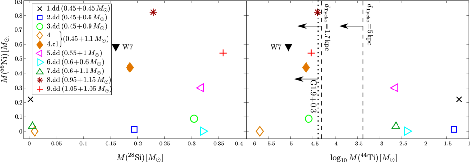
Figure 4: The synthesised mass of $\,\!{}^{56}{\rm Ni}$ (in $M_{\odot}$) as a function of the mass of $\,\!{}^{28}{\rm Si}$ (left) and $\,\!{}^{44}{\rm Ti}$ (right). The three vertical dashed lines in the right panel represent the constraints on the $\,\!{}^{44}{\rm Ti}$ mass for the G1.9+1.3 SN Ia remnant (dotted line; Zoglauer et al., 2015) and the Tycho’s SN Ia remnant (dashed line; Lopez et al., 2015). For Tycho, the upper limits of $\,\!{}^{44}{\rm Ti}$ correspond to range of distance estimates in the literature of $d_{\rm Tycho}=1.7-5.0$ kpc. The filled squared marks the W7, carbon-deflagration model of Nomoto et al. (1984).

Si II $\lambda$ 6355 and Ca II H&K are two strong features in SN Ia spectra. The expansion velocity of the two features are similar and decrease with time as the ejecta is expanding and deeper layers of the ejecta are revealed in the spectra. Foley et al. (2011) have estimated the line velocities of Si II $\lambda$ 6355 and Ca  II  3945(H&K) near maximum brightness and we use their data for 91 SNe Ia to further constrain the detonating models. The SN 2014J and SN 2011fe are also falling within the $2\sigma$ range in the sample of Foley et al. (2011), with $v_{\rm Si\,II}=11.9\times 10^{3}\,{\rm km\,s^{-1}}$ and $v_{\rm Ca\,II}=14.1\times 10^{3}\,{\rm km\,s^{-1}}$ for SN 2014J (Marion et al., 2015) and $v_{\rm Si\,II}=10.4\times 10^{3}\,{\rm km\,s^{-1}}$ for SN 2011fe (no Ca-velocity value given; (Foley & Kirshner, 2013). Figure 5 shows the $\!\,{}^{28}{\rm Si}$ and $\!\,{}^{40}{\rm Ca}$ yields in velocity space obtained for our detonating models together with the $1-$ and $2-\sigma$ lines from the mean of the observed Si and Ca velocities. While the Si II $\lambda$ 6355 velocity near maximum brightness does not vary significantly amongst the observed SNe Ia (within $\pm 2\sigma$ from the mean, $v_{\rm Si,Obs.}$ is in between $8.9$ and $14.3\times 10^{3}\,{\rm km/s}$), Ca II H&K velocity varies significantly (between 8.3 and $20.7\times 10^{3}\,{\rm km/s}$, again, within the $2\sigma$ from the mean).

The mass-weighted mean velocities of Si and Ca of our detonating models (see Table A4) lie close to the lower end of the velocity distribution of the two features, with only 1.dd (both Si and Ca), 2.dd and 6.dd (only Ca) within 2$\sigma$ of the observations. However, the (ionised) mass required to produce a line in the spectra is very low, with values of $\sim\!10^{-6}\,M_{\odot}$ for Ca II and $\sim\!10^{-8}\,M_{\odot}$ for Si II, as computed from Branch et al. (2005) using the data provided in their Table 1 for the optical depths and photosphere velocities corresponding to ten days after the maximum light and an ion population fraction at the lower level of transition of 0.05 (a higher number will further decrease the ion mass required to produce a line). These values can not be used to further constrain the models, as our models produce a total Si and Ca mass calculated between the velocity range of “normal” SNe Ia (i.e., range between $\bar{v}_{\rm Si,Obs}\pm 2\sigma$ and $\bar{v}_{\rm Ca,Obs}\pm 2\sigma$, see Figure 5) between $1.3\times 10^{-5}$ and $4.5\times 10^{-2}\,M_{\odot}$ of Ca and between $9.3\times 10^{-4}$ and $0.15\,M_{\odot}$ of Si. If we exclude run 7.dd (single detonating system, with $0.6+1.1\,M_{\odot}$ components), the lower limit for Ca mass increases to $2.4\times 10^{-4}\,M_{\odot}$.

3.6 Initial conditions

Some models trigger the core detonation only when starting with unrealistic ICs. The model 1.dd ($0.45+0.45\,M_{\odot}$) has to be started with a hotspot inside the core in order to trigger its detonation. This is unrealistic, because, at least when starting with tidally locked WDs, the core is always colder than the surrounding region (envelope), even for equal-mass systems (Dan et al., 2014). Initial conditions for the 5.dd ($0.55+1\,M_{\odot}$) and 7.dd ($0.6+1.1\,M_{\odot}$) models are also not realistic. For these models, there is very little He ($X(\,\!^{4}{\rm He})<0.1$) in the hot envelope and, in order to trigger a detonation, the composition inside the hotspot was artificially set to pure He. In some cases, the energy deposition inside the hotspot required to trigger the core detonation is over a large volume and relatively high. We label the models 1.dd ($0.45+0.45\,M_{\odot}$), 2.dd ($0.45+0.6\,M_{\odot}$) and 8.dd ($0.95+1.15\,M_{\odot}$) as unrealistic, as the energy deposition is within an order of magnitude of the binding energy of the core.

3.7 Constraints on models

	1.dd	2.dd	3.dd	4	4.c1/c2	5.dd	6.dd	7.dd	8.dd	9.dd
	$0.45\!+\!0.45$	$0.45\!+\!0.6$	$0.45\!+\!0.9$	$0.45\!+\!1.1$	$0.45\!+\!1.1$	$0.55\!+\!1$	$0.6\!+\!0.6$	$0.6\!+\!1.1$	$0.95\!+\!1.15$	$1.05\!+\!1.05$
$\!\,{}^{28}{\rm Si}$	✗	✓	✓	✗	✓	✓	✓	✗	✓	✓
$\!\,{}^{40}{\rm Ca}$	✓	✗	✓	✗	✓	✓	✓	✓	✓	✓
$\!\,{}^{44}{\rm Ti}$	✗	✗	✓	✓	✓	✗	✗	✗	✓	✓
$\!\,{}^{56}{\rm Ni}$	✓	✗	✓	✗	✓	✓	✗	✗	✓	✓
ICs	✗a,b)	✗b)	✓	✓	✓	✗c)	✓	✗c)	✗b)	✓

Table 6: Constraints on the models from the observations of $\!\,{}^{44}{\rm Ti}$ mass in the remnants of Tycho (Lopez et al., 2015) and G1.9+0.3 (Zoglauer et al., 2015), $v_{\rm Si}$ and $v_{\rm Ca}$ of “normal” SN Ia sample from Foley et al. (2011), mass of $\!\,{}^{56}{\rm Ni}$ of SN Ia ranging from the sub-luminous SN1991bg up to the bright SN1991T and from how realistic are the initial conditions of each model. $a)$ hotspot placed artificially inside the (cold) dense core and not within the hot envelope which has a low density; $b)$ $0.45+0.45\,M_{\odot}$, $0.45+0.6\,M_{\odot}$ and $0.95+1.15\,M_{\odot}$ have a large, unrealistic initial perturbation; $c)$ because the $0.55+1\,M_{\odot}$ and $0.6+1.1\,M_{\odot}$ models have very little He inside the hot envelope, the composition inside the hotspot is artificially set to pure He.

We compile Table 6 with all the constraints imposed by the nucleosynthetic yields and initial conditions presented above. By strict application of the criteria only three models survive: run 3.dd, an 0.45 He with a $0.9\,M_{\odot}$ CO WD, 4.c1, an 0.45 He with a $1.1\,M_{\odot}$ ONe WD and 9.dd, two $1.05\,M_{\odot}$ CO WDs.

For the 4.c1 run, a detonation is ignited in the $1.1\,M_{\odot}$ ONe core. While the total mass of the remnant is above the Chandrasekhar limit, the region between the core and the disk was shock-heated in the merger and is thermally supported and the (nearly Keplerian) disk is rotationally supported. While the central density of the ONe core (initially $\rho_{\rm max}=3.7\times 10^{7}\,{\rm g\,cm^{-3}}$) is increasing as shocks propagate through the core, it never exceeds $10^{8}\,{\rm g\,cm^{-3}}$. Thus, the collapse to a neutron star can not proceed as the density threshold of the electron captures on the $\!\,{}^{24}{\rm Mg}$ is above $4\times 10^{9}\,{\rm g\,cm^{-3}}$ (in our models $\!\,{}^{24}{\rm Mg}$ is distributed uniformly throughout the core and represents $5\%$ by mass) and for $\!\,{}^{20}{\rm Ne}$ is even higher, at above $9\times 10^{9}\,{\rm g\,cm^{-3}}$ (Miyaji et al., 1980; Saio & Nomoto, 1985). For the 4.c1 model, the shock waves from the initial He detonation converge inside the core and raise the temperature to $T\approx 6\times 10^{9}$ K at a density of $\rho\approx 4\times 10^{7}\,{\rm g\,cm^{-3}}$ over a radius of $(100\ {\rm km})$ located at the pole ($r\approx 0$ km). This triggers a second detonation into the core. Sufficient energy is released in the nuclear burning ($9.427\times 10^{50}$ erg) to unbind the ONe core (binding energy of $3.879\times 10^{50}$ erg). However, the ONe detonations are not yet proven to work as there are no calculations of resolved ONe detonation structures (weaker shocks could yield a detonation in unresolved simulations compared to resolved ones), with the recent study of Shen & Bildsten (2014) arguing against this possibility due to the increased detonation length- and shock-strength required to trigger a detonation.

Recently, Marquardt et al. (2015) have studied the detonations of massive, ONe WDs under the assumptions that they ignite at the center of the star. Compared to our models, they start with larger masses, between 1.18 and $1.23\,M_{\odot}$, and they are not the remnants of a merger process, but “naked”, hydrostatic WDs. Their synthetic light curves do not match the observations of a “normal” SN Ia, owing to their large $\!\,{}^{56}{\rm Ni}$ masses, but show better agreement with the “over-luminous” SN 1991T. Inversely, due to the strong SI II and Ca II absorption lines shown in the models, the spectra show better agreement with those of “normal” SN Ia than with those of SN 1991T. While we can not compare directly to their calculations, we point out that it is encouraging to note that in our 4.c1 model there is less $\!\,{}^{56}{\rm Ni}$ produced, within the range of SNe Ia.

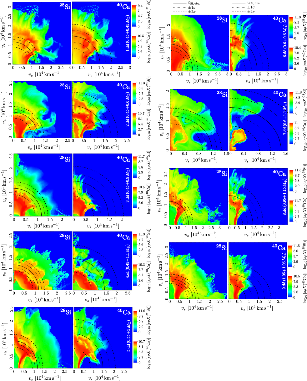
Figure 5: $\!\,{}^{28}{\rm Si}$ and $\!\,{}^{40}{\rm Ca}$ ($s\rho X_{i}$, in logarithmic scale; final units are ${\rm g\,cm^{-2}}$, the same as in Figure 3, and the snapshots are again taken after $t=39\,{\rm s}$) for all remnant models. Overplotted is the mean (continuous line) $1-$ (dotted line) and $2-\sigma$ (dashed lines) of the observed Si and Ca velocities near maximum brightness for 91 SNe Ia (Foley et al., 2011).

There are strong orientation effects for most of the models as the nuclear burning products are moving faster in the polar direction (Figure 6 and 7). The asymmetries are caused by the location where the detonation is triggered in the envelope/core, the slowing of the ejecta by the surrounding disk, concentrated in the equatorial plane and by the rotation. The light curves resulting from these models would likely show a non-negligible sensitivity to line-of-sight effects (see a detailed discussion on the line-of-sight effects for asymmetric ejecta in Moll & Woosley, 2013).

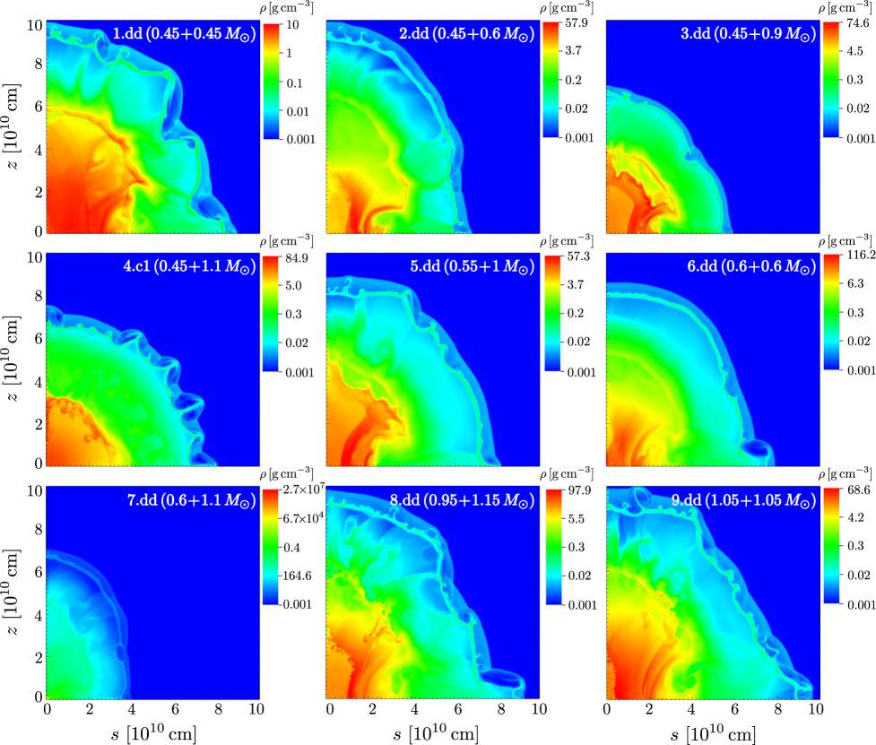
Figure 6: Density structure of all remnants. The energetics of the ejecta is imprinted in the extension of the shock front at the contact surface between the ejecta and the low-density ambient matter. This is why we had to take the final snapshots after $t=39$ s from the beginning of the simulations, when for the runs with largest kinetic energy the ejecta reach the grid boundaries at $10^{11}$ km. For the models shown here a core detonation occurs for all but the $0.6+1.1\,M_{\odot}$ system. The ejecta of the explosion has to propagate through an environment spanning a wide range of densities: from the dense, nearly Keplerian-rotating disk to the low density of the ambient. This is naturally resulting in an asymmetric shock front, more extended towards the pole and in developing Rayleigh-Taylor hydrodynamic instabilities behind the shock front, when the denser layers penetrate the overlying lighter ambient environment.

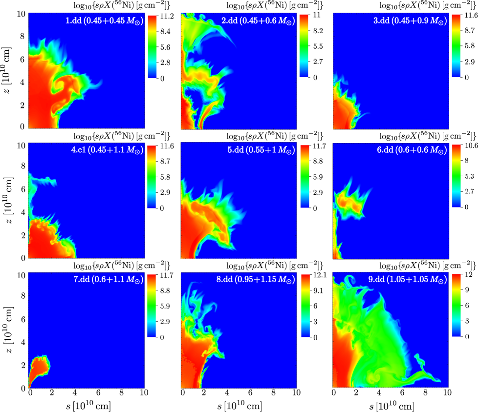
Figure 7: $\,\!{}^{56}{\rm Ni}$ mass fraction distribution (scaled with $s\rho$; in logarithmic scale; units are the same as in Figure 3) of all remnants. Similar to the density structure of the remnants (Figure 6) the snapshots were taken after $t=39$ s from the beginning of the simulations and the boundary of the domain is at $10^{11}$ km. As seen in the density structure, the asymmetric shock front causes a more extended $\,\!{}^{56}{\rm Ni}$ distribution towards the pole.

4 Summary

We have studied 2D detonation models of WD-WD merger remnants using the Eulerian AMR code FLASH. Our initial conditions here are based on the remnant structures from our earlier 3D SPH simulations (Dan et al., 2014). In total we consider nine systems that cover the entire range of WD masses and compositions. For each of these systems, we modeled the initiation and propagation of detonations and followed the nucleosynthesis processes until the ejecta reached the homologous phase.

After the restart of the simulations with FLASH only the $0.45+1.1\,M_{\odot}$ model (run 4) triggered a detonation in the hot envelope, but it did not lead to a second detonation in the underlying core. The envelope detonation produced almost no $\!\,{}^{56}{\rm Ni}$ and very little other radioactive elements. Note, however, the results for this set of runs should be regarded as lower limits. There are two main reasons that these models do not detonate. First, the 3D SPH calculations were done at a moderate resolution and, in reality, mergers will produce remnants that are more prone to explosion than our finite resolution results. Secondly, there is a loss of resolution after the mapping onto the grid. This has an impact onto the thermal evolution of the remnant as the hotspots in the hot envelope surrounding the relatively cold core are smoothed out. Chemical compositions are also deteriorated by the mapping process, especially inside chemically mixed regions. This motivated two more sets of runs, with different setups for the initiation of a detonation being tested. In one set of models, we manually setup hotspots in the remnant’s envelopes based on the realistic conditions found in the 3D SPH simulations. In another set of models, the hotspots were setup based on the conditions for direct detonation initiation taken from the results of spatially resolved 1D calculations from the literature. It is in this later set of models that all systems trigger a detonation, whether it is only an envelope detonation or the core is ignited as well.

With perturbations based on the several SPH criteria, again only the $0.45+1.1\,M_{\odot}$ system detonates, but this time the envelope detonation is strong enough so that a second detonation occurs in the ONe core. The model which leads to a double detonation, run 4.c1, starts with a hotspot at the location where the ratio $\tau_{\rm nuc}/\tau_{\rm dyn}(T)$ is minimum. The hotspot’s temperature is the same with the temperature of the SPH particle with minimum ratio.

With perturbations following the critical conditions for a direct initiation of a detonation from the spatially resolved 1D calculations, all systems detonate. Three possible outcomes were found: a detonation is triggered in the envelope but a second detonation in the core is avoided (run 7.dd); a detonation is not ignited in the envelope but the shock waves from the initial perturbation converge inside the core and trigger a detonation there (run 6.dd and runs with CO mass transferring systems, 8.dd and 9.dd); for the other models a detonations occur, both, in the He shell and the CO/ONe core. However, in some cases the initial conditions are unrealistic and we reject these models as viable SNe Ia progenitor candidates.

The nucleosynthetic yields of the successfully detonating models have been compared with the observations of SNe Ia and their subsequent constraints have been applied to the WD-WD merger scenario. Only three models survive all constraints and potentially lead to a SN Ia event: $0.45\,M_{\odot}$ He and $0.9\,M_{\odot}$ CO WD that produces little $\!\,{}^{56}{\rm Ni}$ and could possibly result in a sub-luminous, SN 1991bg-like event and two good candidates for reproducing common SNe Ia, $0.45\ M_{\odot}$ He with a $1.1\,M_{\odot}$ ONe WD and a double CO WD system with two $1.05\,M_{\odot}$ components. The last two models have in common a former accretor with a mass $M>1\,M_{\odot}$, while the last model has a total mass well above the Chandrasekhar limit. There is observational evidence that such massive WDs exist and they form a mass excess in the mass distribution (e.g., Liebert et al., 2005; Ferrario et al., 2005). Population synthesis calculations of Fryer et al. (2010) also predict that over one third of the systems with a total mass above the Chandrasekhar mass limit have $M_{\rm tot}\gtrsim 1.8\,M_{\odot}$. However, they do not dominate the current SN Ia sample being less common than systems with a combined mass near the Chandrasekhar limit (Toonen et al., 2012), such as the $0.45+0.9\,M_{\odot}$ system. Our results confirm that WD-WD mergers can show reasonable agreement with the observed nucleosynthesis of SNe Ia and a variety of outcomes are possible, covering essentially the entire range of observed supernovae that are associated with thermonuclear explosions.

Acknowledgments

We thank the reviewer for his/her valuable comments and suggestions that improved the manuscript. We thank Laura Lopez, Jerod Parrent, Danny Milisavljevic, Lev Yungelson and Philipp Podsiadlowski for discussions and for suggesting useful references. This work was supported by Einstein grant PF3-140108 (J. G.), the Packard grant (E. R.), NASA ATP grant NNX14AH37G (E. R.). and the Swedish Research Council (VR) under grant 621-2012-4870 (S. R.). The FLASH code was developed in part by the DOE-supported Alliances Center for Astrophysical Thermonuclear Flashes (ASC) at the University of Chicago.

.1 Initial conditions

Run	Initial	Initial	$T_{\rm max,8}$	$\rho_{5}(T_{\rm max})$
No	masses [$M_{\odot}$]	compositions
Helium mass transferring systems
1	$0.45+0.45$	He-He	0.990	0.543
2	$0.45+0.6$	He-HeCO	1.934	0.436
3	$0.45+0.9$	He-CO	4.799	0.201
4	$0.45+1.1$	He-ONe	5.235	3.872
5	$0.55+1$	HeCO-CO	5.384	3.941
6	$0.6+0.6$	HeCO-HeCO	3.341	0.720
7	$0.6+1.1$	HeCO-CO	7.218	6.354
Carbon/oxygen mass transferring systems
8	$0.95+1.15$	CO-ONe	9.693	7.411
9	$1.05+1.05$	CO-CO	7.844	19.523

Table A1: Initial conditions of the first set of runs, without perturbations: $T_{\rm max,8}$ (in units of $10^{8}$ K) and $\rho_{5}(T_{\rm max})$ (in units of $10^{5}\,{\rm g/cm^{-3}}$) are the maximum temperature and density at the location of maximum temperature, respectively. The masses (in $M_{\odot}$) and compositions are those from the beginning of the SPH calculations.

Run	Initial	Initial	$s_{\rm per,9}$	$z_{\rm per,9}$	$T_{\rm per,8}$	$\rho_{5}(T_{\rm per})$	hotspot	Comments
No	masses [$M_{\odot}$]	compositions					criteria
Helium mass transferring systems
1.c1	$0.45+0.45$	He-He	0.403	0.661	1.01	0.776	$C_{1}$	quadrant I
1.c2	$0.45+0.45$	He-He	0.460	0.882	1.292	0.100	$C_{2}$	quadrant I
1.c3	$0.45+0.45$	He-He	0.247	0.653	1.219	1.107	$C_{3}$	quadrant I
2.c1	$0.45+0.6$	He-HeCO	0.744	0.162	1.980	1.976	$C_{1}$	quadrant IV
2.c2	$0.45+0.6$	He-HeCO	0.532	0.773	2.336	0.196	$C_{2}$	quadrant I
2.c3	$0.45+0.6$	He-HeCO	0.703	0.389	2.092	1.085	$C_{3}$	quadrant I
3.c1/c3	$0.45+0.9$	He-CO	0.681	0.029	5.525	1.229	$C_{1},\,C_{3}$	quadrant I
3.c2	$0.45+0.9$	He-CO	0.395	0.645	5.948	0.313	$C_{2}$	quadrant I
4.c1/c2	$0.45+1.1$	He-ONe	0.595	0.026	6.810	0.895	$C_{1}$	quadrant I
4.c3	$0.45+1.1$	He-ONe	0.575	0.034	4.698	1.166	$C_{3}$	no run, as $T_{\rm per}\approx T_{\rm grid}$
5.c1/c2/c3	$0.55+1$	HeCO-CO	0.607	0.009	9.790	2.320	$C_{1},\,C_{2},\,C_{3}$	quadrant IV
6.c1/c2/c3	$0.6+0.6$	HeCO-HeCO	0.725	0.307	3.670	1.629	$C_{1},\,C_{2},\,C_{3}$	quadrant IV
7.c1/c3	$0.6+1.1$	HeCO-CO	0.640	0.085	4.640	1.282	$C_{1},\,C_{3}$	quadrant IV
7.c2	$0.6+1.1$	HeCO-CO	0.818	0.131	6.243	0.544	$C_{2}$	quadrant I
Carbon/oxygen mass transferring systems
8.c1	$0.95+1.15$	CO - ONe	0.295	0.173	11.6	28.525	$C_{1}$	quandrant IV
8.c2/c4	$0.95+1.15$	CO - ONe	0.278	0.248	11.738	14.898	$C_{2},\,C_{4}$	quadrant I
9.c1/c2/c4	$1.05+1.05$	CO-CO	0.405	0.029	10.407	34.661	$C_{1},\,C_{2},\,C_{4}$	quadrant IV

Table A2: Initial conditions for the second set of runs, with perturbations based on different criteria guided by the 3D SPH simulations. $s_{\rm per,9}$ and $z_{\rm per,9}$ are the coordinates on the $s$– and $z$–axis where the hotspot’s center is placed, respectively, $T_{\rm per,8}$ is the perturbation temperature (in units of $10^{8}\,{\rm K}$) and $\rho_{5}(T_{\rm per})$ is the density at the location of the perturbation (in units of $10^{5}\,{\rm g\,cm^{-3}}$). The hotspot criteria labelling is explained in Section 2.1.

We run three sets of simulations, with and without a temperature perturbation. Table A1 shows the initial conditions for the first set of runs, without temperature perturbations. The initial conditions for the second set of runs, where temperature perturbations are set based on different criteria guided by the 3D SPH simulations, are given in Table A2. For the third set of runs, the temperature perturbations are setup following the critical conditions for a spontaneous initiation of a detonation from the spatially resolved 1D calculations of Holcomb et al. (2013) and Shen & Moore (2014) for He composition and Röpke et al. (2007) and Seitenzahl et al. (2009) for CO and the initial conditions are given in Table A3.

Runs are ordered by increasing donor’s mass and by decreasing mass ratio $q$ and labeled 1 through 9. For the second and third set of runs, we have added to the run number the hotspot search criteria and a “.dd”, respectively.

Run	Initial	Initial	$s_{\rm per,9}$	$z_{\rm per,9}$	$T_{\rm per,8}$	$\rho_{5}(T_{\rm per})$	Comments
No	masses [$M_{\odot}$]	compositions
Helium mass transferring systems
1.dd	$0.45+0.45$	He-He	0.546	0.184	5.0	5.012	unrealistic ICs: hotspot inside
							cold (dense) core
2.dd	$0.45+0.6$	He-HeCO	0.576	0.166	5.0	5.002
2.dd-Polar	$0.45+0.6$	He-HeCO	0.0	0.522	5.0	5.045
3.dd	$0.45+0.9$	He-CO	0.584	0.071	8.0	3.008
3.dd-Polar	$0.45+0.9$	He-CO	0.0	0.593	8.0	1.713
5.dd	$0.55+1.0$	HeCO-CO	0.322	0.369	8.0	5.011	hotspot composition set to $X(\!\,^{4}{\rm He})=1$,
							as $X(\!\,^{4}{\rm He})<0.1$ at $\rho\geq 6\times 10^{4}\,{\rm g\,cm^{-3}}$
6.dd	$0.6+0.6$	HeCO-HeCO	0.225	0.539	5.0	3.011
7.dd	$0.6+1.1$	HeCO-ONe	0.387	0.238	-	5.966	No perturb., but pure He at ($s_{\rm per},z_{\rm per}$),
							as $X(\!\,^{4}{\rm He})<0.1$ at $\rho\geq 3.9\times 10^{4}\,{\rm g\,cm^{-3}}$
Carbon/oxygen mass transferring systems
8.dd	$0.95+1.15$	CO-ONe	0.341	0.083	30.0	30.313
9.dd	$1.05+1.05$	CO-CO	0.135	0.308	30.0	19.923

Table A3: Initial conditions for the third set of runs, using the critical conditions for a spontaneous initiation of a detonation from the spatially resolved 1D calculations of Holcomb et al. (2013) and Shen & Moore (2014) for He composition and Röpke et al. (2007) and Seitenzahl et al. (2009) for CO. Same quantities as in Table A2, only labelling has been changed, with “dd” added after the run number.

.2 Nucleosynthetic yields

The nucleosynthetic yields and kinetic energies for all the models that detonated. Run 4 is the only run without a perturbation where a single, He-detonation is triggered, while for run 4.c1/c2, with a perturbation of $R_{\rm per}=500\,{\rm km}$ at the location where the ratio $\tau_{\rm nuc}/\tau_{\rm dyn}(T)$ is minimum in the SPH calculations, a double detonation is triggered. Runs labelled with “dd” after the number are those where the hotspots are setup following the critical conditions for a direct initiation of a detonation from the spatially resolved 1D calculations. For this set of runs, for all models but 7.dd a detonation is triggered in the core.

	1.dd	2.dd	3.dd	4	4.c1/c2	5.dd	6.dd	7.dd	8.dd	9.dd
	$0.45\!+\!0.45$	$0.45\!+\!0.6$	$0.45\!+\!0.9$	$0.45\!+\!1.1$	$0.45\!+\!1.1$	$0.55\!+\!1$	$0.6\!+\!0.6$	$0.6\!+\!1.1$	$0.95\!+\!1.15$	$1.05\!+\!1.05$
$\!\,{}^{4}{\rm He}$	$4.95(-1)$	$4.03(-1)$	$4.14(-1)$	$3.67(-1)$	$4.47(-2)$	$8.73(-2)$	$8.05(-2)$	$9.45(-2)$	$8.55(-3)$	$4.34(-3)$
$\!\,{}^{12}{\rm C}$	$9.83(-3)$	$1.54(-2)$	$7.03(-2)$	$2.77(-2)$	$7.13(-3)$	$1.91(-1)$	$2.35(-1)$	$2.27(-1)$	$2.04(-1)$	$1.94(-1)$
$\!\,{}^{16}{\rm O}$	$1.33(-5)$	$1.57(-1)$	$2.13(-1)$	$6.39(-1)$	$1.83(-1)$	$2.76(-1)$	$2.54(-1)$	$8.27(-1)$	$5.95(-1)$	$6.21(-1)$
$\!\,{}^{20}{\rm Ne}$	$3.44(-5)$	$2.11(-3)$	$2.08(-2)$	$3.84(-1)$	$8.95(-2)$	$6.14(-2)$	$7.30(-2)$	$3.94(-1)$	$4.75(-2)$	$2.72(-2)$
$\!\,{}^{24}{\rm Mg}$	$8.08(-5)$	$6.35(-2)$	$3.53(-2)$	$6.34(-2)$	$2.65(-2)$	$4.62(-2)$	$1.56(-1)$	$6.28(-2)$	$4.38(-2)$	$6.22(-2)$
$\!\,{}^{28}{\rm Si}$	$2.3(-3)$	$1.94(-1)$	$3.04(-1)$	$1.02(-2)$	$1.86(-1)$	$3.17(-1)$	$3.21(-1)$	$5.87(-3)$	$2.29(-1)$	$3.58(-1)$
$\!\,{}^{32}{\rm S}$	$3.2(-3)$	$4.46(-2)$	$1.5(-1)$	$3.52(-3)$	$1.13(-1)$	$1.63(-1)$	$4.79(-2)$	$7.31(-4)$	$1.09(1)$	$1.64(-1)$
$\!\,{}^{36}{\rm Ar}$	$7.18(-3)$	$2.29(-2)$	$2.89(-2)$	$1.01(-3)$	$2.36(-2)$	$3.14(-2)$	$9.45(-3)$	$5.63(-4)$	$2.17(-2)$	$3.07(-2)$
$\!\,{}^{40}{\rm Ca}$	$3.25(-2)$	$5.48(-2)$	$2.35(-2)$	$1.55(-4)$	$2.35(-2)$	$2.97(-2)$	$4.69(-3)$	$2.08(-3)$	$2.12(-2)$	$2.82(-2)$
$\!\,{}^{44}{\rm Ti}$	$6.14(-2)$	$4.66(-2)$	$2.53(-5)$	$2.02(-6)$	$2.21(-5)$	$2.21(-3)$	$4.13(-3)$	$2.31(-3)$	$4.01(-5)$	$2.91(-5)$
$\!\,{}^{48}{\rm Cr}$	$3.8(-2)$	$2.22(-2)$	$1.80(-4)$	$2.13(-9)$	$3.46(-4)$	$2.23(-3)$	$3.62(-3)$	$1.91(-3)$	$3.03(-4)$	$3.12(-4)$
$\!\,{}^{52}{\rm Fe}$	$3.5(-2)$	$9.27(-3)$	$3.12(-3)$	$4.68(-13)$	$8.29(-3)$	$9.95(-3)$	$1.62(-3)$	$4.93(-3)$	$6.65(-3)$	$6.59(-3)$
$\!\,{}^{56}{\rm Ni}$	$2.21(-1)$	$1.25(-2)$	$8.76(-2)$	$3.37(-13)$	$4.41(-1)$	$3.01(-1)$	$6.81(-4)$	$3.48(-2)$	$8.22(-1)$	$5.41(-1)$
$28\!\leq\!A\!\leq\!40$	0.045	0.158	0.506	0.015	0.346	0.54	0.383	0.009	0.38	0.581
$A\geq 44$	0.355	0.045	0.091	2.019(-6)	0.45	0.315	0.01	0.044	0.829	0.548
$E_{\rm kin}$	$1.09(51)$	$7.54(50)$	$6.76(50)$	$1.75(49)$	$6.87(50)$	$1.05(51)$	$7.46(50)$	$9.08(49)$	$7.149(50)$	$1.27(51)$
$\langle v_{\rm Si}\rangle$	11.2	5.4	5.6	1.4	8.4	8.2	6.8	5.5	8.1	7.4
$\langle v_{\rm Ca}\rangle$	11.5	9.9	4.9	1.5	7.5	7.6	8.4	6.8	7.6	6.8

Table A4: Isotope yields (by mass, in units of $M_{\odot}$), kinetic energies (in units of $\rm{erg}$) and the Si and Ca mass-weighted velocities (in units of $10^{3}\,{\rm km/s}$) for all runs where detonations are triggered. Below the run numbers are the initial masses (in $M_{\odot}$) of the two stars. The floating-point numbers are expressed in the form significand followed in the brackets by the exponent of the base 10.

References

- Arnett (1982) Arnett W. D., 1982, ApJ, 253, 785
- Aznar-Siguán et al. (2013) Aznar-Siguán G., García-Berro E., Lorén-Aguilar P., José J., Isern J., 2013, MNRAS, 434, 2539
- Bildsten et al. (2007) Bildsten L., Shen K. J., Weinberg N. N., Nelemans G., 2007, ApJL, 662, L95
- Blondin et al. (2015) Blondin S., Dessart L., Hillier D. J., 2015, MNRAS, 448, 2766
- Borkowski et al. (2010) Borkowski K. J., Reynolds S. P., Green D. A., Hwang U., Petre R., Krishnamurthy K., Willett R., 2010, ApJL, 724, L161
- Branch et al. (2005) Branch D., Baron E., Hall N., Melakayil M., Parrent J., 2005, PASP, 117, 545
- Churazov et al. (2014) Churazov E. et al., 2014, Nature, 512, 406
- Couch et al. (2013) Couch S. M., Graziani C., Flocke N., 2013, ApJ, 778, 181
- Dan et al. (2014) Dan M., Rosswog S., Brüggen M., Podsiadlowski P., 2014, MNRAS, 438, 14
- Dan et al. (2012) Dan M., Rosswog S., Guillochon J., Ramirez-Ruiz E., 2012, MNRAS, 422, 2417
- Ferrario et al. (2005) Ferrario L., Wickramasinghe D., Liebert J., Williams K. A., 2005, MNRAS, 361, 1131
- Fink et al. (2007) Fink M., Hillebrandt W., Röpke F. K., 2007, A&A, 476, 1133
- Foley & Kirshner (2013) Foley R. J., Kirshner R. P., 2013, ApJL, 769, L1
- Foley et al. (2011) Foley R. J., Sanders N. E., Kirshner R. P., 2011, ApJ, 742, 89
- Fossey et al. (2014) Fossey J., Cooke B., Pollack G., Wilde M., Wright T., 2014, CBET, 3792, 1
- Fryer et al. (2010) Fryer C. L. et al., 2010, ApJ, 725, 296
- Fryxell et al. (2000) Fryxell B. et al., 2000, ApJS, 131, 273
- Fryxell et al. (1989) Fryxell B. A., Müller E., Arnett W. D., 1989, MPA Green Report, Max-Planck-Institut für Astrophysik Garching, 449
- García-Senz et al. (1999) García-Senz D., Bravo E., Woosley S. E., 1999, A&A, 349, 177
- García-Senz et al. (2013) García-Senz D., Cabezón R. M., Arcones A., Relaño A., Thielemann F. K., 2013, MNRAS, 436, 3413
- Guerrero et al. (2004) Guerrero J., García-Berro E., Isern J., 2004, A&A, 413, 257
- Guillochon et al. (2010) Guillochon J., Dan M., Ramirez-Ruiz E., Rosswog S., 2010, ApJL, 709, L64
- Hawley et al. (2012) Hawley W. P., Athanassiadou T., Timmes F. X., 2012, ApJ, 759, 39
- Hillebrandt & Niemeyer (2000) Hillebrandt W., Niemeyer J. C., 2000, ARAA, 38, 191
- Holcomb et al. (2013) Holcomb C., Guillochon J., De Colle F., Ramirez-Ruiz E., 2013, ApJ, 771, 14
- Howell (2011) Howell D. A., 2011, Nature Communications, 2
- Iben & Tutukov (1984) Iben, Jr. I., Tutukov A. V., 1984, ApJS, 54, 335
- Kashi & Soker (2011) Kashi A., Soker N., 2011, MNRAS, 417, 1466
- Kashyap et al. (2015) Kashyap R., Fisher R., García-Berro E., Aznar-Siguán G., Ji S., Lorén-Aguilar P., 2015, ApJL, 800, L7
- Kushnir et al. (2013) Kushnir D., Katz B., Dong S., Livne E., Fernández R., 2013, ApJL, 778, L37
- Li et al. (2011) Li W. et al., 2011, MNRAS, 412, 1441
- Liebert et al. (2005) Liebert J., Bergeron P., Holberg J. B., 2005, ApJS, 156, 47
- Livio & Riess (2003) Livio M., Riess A. G., 2003, ApJL, 594, L93
- Livne (1990) Livne E., 1990, ApJL, 354, L53
- Livne & Arnett (1995) Livne E., Arnett D., 1995, ApJ, 452, 62
- Lopez et al. (2015) Lopez L. A. et al., 2015, ArXiv e-prints, arXiv:1504.07238
- Luminet & Pichon (1989) Luminet J.-P., Pichon B., 1989, A&A, 209, 103
- MacNeice et al. (2000) MacNeice P., Olson K. M., Mobarry C., de Fainchtein R., Packer C., 2000, Computer Physics Communications, 126, 330
- Maoz et al. (2014) Maoz D., Mannucci F., Nelemans G., 2014, ARA&A, 52, 107
- Marion et al. (2015) Marion G. H. et al., 2015, ApJ, 798, 39
- Marquardt et al. (2015) Marquardt K. S., Sim S. A., Ruiter A. J., Seitenzahl I. R., Ohlmann S. T., Kromer M., Pakmor R., Röpke F. K., 2015, A&A, 580, A118
- Mazzali et al. (2007) Mazzali P. A., Röpke F. K., Benetti S., Hillebrandt W., 2007, Science, 315, 825
- Mazzali et al. (2008) Mazzali P. A., Sauer D. N., Pastorello A., Benetti S., Hillebrandt W., 2008, MNRAS, 386, 1897
- Mazzali et al. (2015) Mazzali P. A. et al., 2015, MNRAS, 450, 2631
- Miyaji et al. (1980) Miyaji S., Nomoto K., Yokoi K., Sugimoto D., 1980, PASJ, 32, 303
- Moll & Woosley (2013) Moll R., Woosley S. E., 2013, ApJ, 774, 137
- Nomoto (1982a) Nomoto K., 1982a, ApJ, 257, 780
- Nomoto (1982b) Nomoto K., 1982b, ApJ, 253, 798
- Nomoto et al. (1984) Nomoto K., Thielemann F.-K., Yokoi K., 1984, ApJ, 286, 644
- Nugent et al. (2011) Nugent P. E. et al., 2011, Nature, 480, 344
- Pakmor et al. (2010) Pakmor R., Kromer M., Röpke F. K., Sim S. A., Ruiter A. J., Hillebrandt W., 2010, Nature, 463, 61
- Pakmor et al. (2012) Pakmor R., Kromer M., Taubenberger S., Sim S. A., Röpke F. K., Hillebrandt W., 2012, ApJL, 747, L10
- Pakmor et al. (2013) Pakmor R., Kromer M., Taubenberger S., Springel V., 2013, ApJL, 770, L8
- Papatheodore & Messer (2014) Papatheodore T. L., Messer O. E. B., 2014, ApJ, 782, 12
- Papish & Perets (2015) Papish O., Perets H. B., 2015, ArXiv e-prints, arXiv:1502.03453
- Pereira et al. (2013) Pereira R. et al., 2013, A&A, 554, A27
- Perlmutter et al. (1998) Perlmutter S. et al., 1998, Nature, 391, 51
- Phillips (1993) Phillips M. M., 1993, ApJL, 413, L105
- Piro et al. (2014) Piro A. L., Thompson T. A., Kochanek C. S., 2014, MNRAS, 438, 3456
- Postnov & Yungelson (2014) Postnov K. A., Yungelson L. R., 2014, Living Rev. in Relativ., 17, 3
- Raskin et al. (2014) Raskin C., Kasen D., Moll R., Schwab J., Woosley S., 2014, ApJ, 788, 75
- Raskin et al. (2012) Raskin C., Scannapieco E., Fryer C., Rockefeller G., Timmes F. X., 2012, ApJ, 746, 62
- Raskin et al. (2009) Raskin C., Timmes F. X., Scannapieco E., Diehl S., Fryer C., 2009, MNRAS, 399, L156
- Reynolds et al. (2008) Reynolds S. P., Borkowski K. J., Green D. A., Hwang U., Harrus I., Petre R., 2008, ApJL, 680, L41
- Riess et al. (1998) Riess A. G. et al., 1998, AJ, 116, 1009
- Röpke et al. (2007) Röpke F. K., Woosley S. E., Hillebrandt W., 2007, ApJ, 660, 1344
- Rosswog et al. (2009a) Rosswog S., Kasen D., Guillochon J., Ramirez-Ruiz E., 2009a, ApJL, 705, L128
- Rosswog et al. (2009b) Rosswog S., Ramirez-Ruiz E., Hix W. R., 2009b, ApJ, 695, 404
- Roy & Pal (2014) Roy S., Pal S., 2014, in IAU Symposium, Vol. 296, IAU Symposium, Ray A., McCray R. A., eds., pp. 197–201
- Saio & Nomoto (1985) Saio H., Nomoto K., 1985, A&A, 150, L21
- Sasdelli et al. (2014) Sasdelli M., Mazzali P. A., Pian E., Nomoto K., Hachinger S., Cappellaro E., Benetti S., 2014, MNRAS, 445, 711
- Sato et al. (2015) Sato Y., Nakasato N., Tanikawa A., Nomoto K., Maeda K., Hachisu I., 2015, ApJ, 807, 105
- Seitenzahl et al. (2009) Seitenzahl I. R., Meakin C. A., Townsley D. M., Lamb D. Q., Truran J. W., 2009, ApJ, 696, 515
- Shen & Bildsten (2009) Shen K. J., Bildsten L., 2009, APJ, 699, 1365
- Shen & Bildsten (2014) Shen K. J., Bildsten L., 2014, ApJ, 785, 61
- Shen et al. (2010) Shen K. J., Kasen D., Weinberg N. N., Bildsten L., Scannapieco E., 2010, ApJ, 715, 767
- Shen & Moore (2014) Shen K. J., Moore K., 2014, ApJ, 797, 46
- Sim et al. (2012) Sim S. A., Fink M., Kromer M., Röpke F. K., Ruiter A. J., W., 2012, MNRAS, 420, 3003
- Sim et al. (2010) Sim S. A., Röpke F. K., Hillebrandt W., Kromer M., Pakmor R., Fink M., Ruiter A. J., Seitenzahl I. R., 2010, ApJL, 714, L52
- Stehle et al. (2005) Stehle M., Mazzali P. A., Benetti S., Hillebrandt W., 2005, MNRAS, 360, 1231
- Stritzinger et al. (2006) Stritzinger M., Mazzali P. A., Sollerman J., Benetti S., 2006, A&A, 460, 793
- Tanaka et al. (2011) Tanaka M., Mazzali P. A., Stanishev V., Maurer I., Kerzendorf W. E., Nomoto K., 2011, MNRAS, 410, 1725
- Timmes (1999) Timmes F. X., 1999, ApJS, 124, 241
- Timmes & Swesty (2000) Timmes F. X., Swesty F. D., 2000, ApJS, 126, 501
- Toonen et al. (2012) Toonen S., Nelemans G., Portegies Zwart S., 2012, A&A, 546, A70
- Tsebrenko & Soker (2015) Tsebrenko D., Soker N., 2015, MNRAS, 447, 2568
- Waldman et al. (2011) Waldman R., Sauer D., Livne E., Perets H., Glasner A., Mazzali P., Truran J. W., Gal-Yam A., 2011, ApJ, 738, 21
- Wang & Han (2012) Wang B., Han Z., 2012, NewAR, 56, 122
- Webbink (1984) Webbink R. F., 1984, ApJ, 277, 355
- Whelan & Iben (1973) Whelan J., Iben, Jr. I., 1973, ApJ, 186, 1007
- Woosley & Kasen (2011) Woosley S. E., Kasen D., 2011, ApJ, 734, 38
- Woosley & Weaver (1994) Woosley S. E., Weaver T. A., 1994, ApJ, 423, 371
- Yamaguchi et al. (2014) Yamaguchi H. et al., 2014, ApJL, 785, L27
- Yoon et al. (2007) Yoon S., Podsiadlowski P., Rosswog S., 2007, MNRAS, 380, 933
- Zhu et al. (2013) Zhu C., Chang P., van Kerkwijk M. H., Wadsley J., 2013, ApJ, 767, 164
- Zoglauer et al. (2015) Zoglauer A. et al., 2015, ApJ, 798, 98